Embed Size (px)
Citation preview
Numerical and Experimental Study of Mixing Processes Associated with Hydrogen and
High Hydrogen Content Fuels
October 19, 2010
Amin Akbari, Scott Hill, Patrick Randall, and Vincent McDonell
Mark Freeman and Richard Dennis
19 October 2009 2/48
Outline
• Motivation
• Project Goals
• Progress to Date
– Experimental Study
– Numerical Study
• Next Steps
19 October 2009 3/48
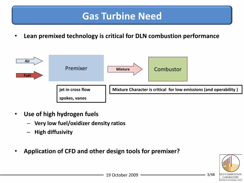
Gas Turbine Need
• Lean premixed technology is critical for DLN combustion performance
• Use of high hydrogen fuels
– Very low fuel/oxidizer density ratios
– High diffusivity
• Application of CFD and other design tools for premixer?
Air
Fuel
Premixer Mixture Combustor
jet in cross flow
spokes, vanes
Mixture Character is critical for low emissions (and operability )
19 October 2009 4/48
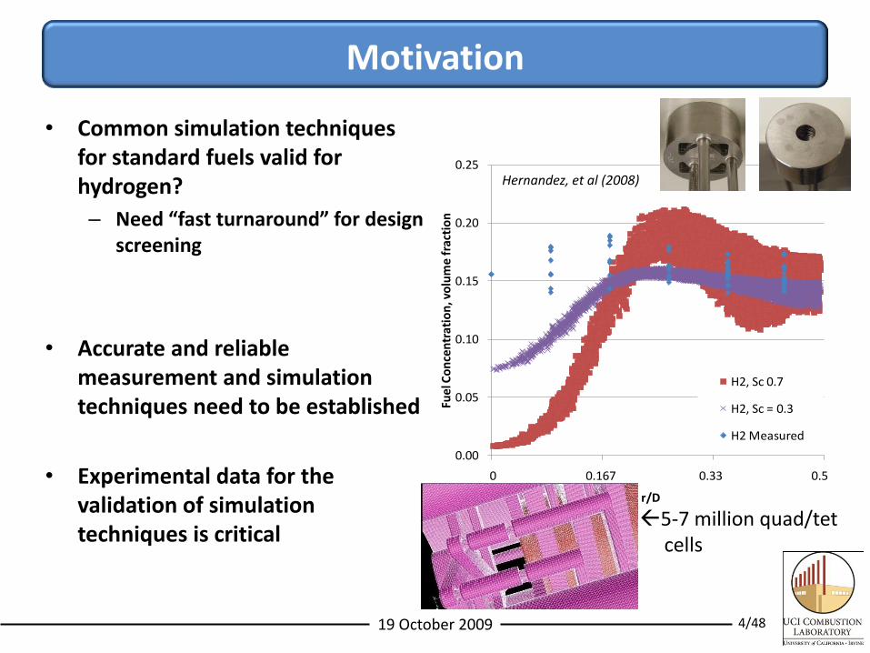
Motivation
• Common simulation techniques for standard fuels valid for hydrogen?
– Need “fast turnaround” for design screening
• Accurate and reliable measurement and simulation techniques need to be established
• Experimental data for the validation of simulation techniques is critical
0.00
0.05
0.10
0.15
0.20
0.25
0 0.001 0.002 0.003
Fuel
Co
nce
ntr
atio
n, v
olu
me
frac
tio
n
Radial Position, m
H2, Sc 0.7
H2, Sc = 0.3
H2 Measured
0 0.167 0.33 0.5
r/D
Hernandez, et al (2008)
5-7 million quad/tetcells
19 October 2009 5/48
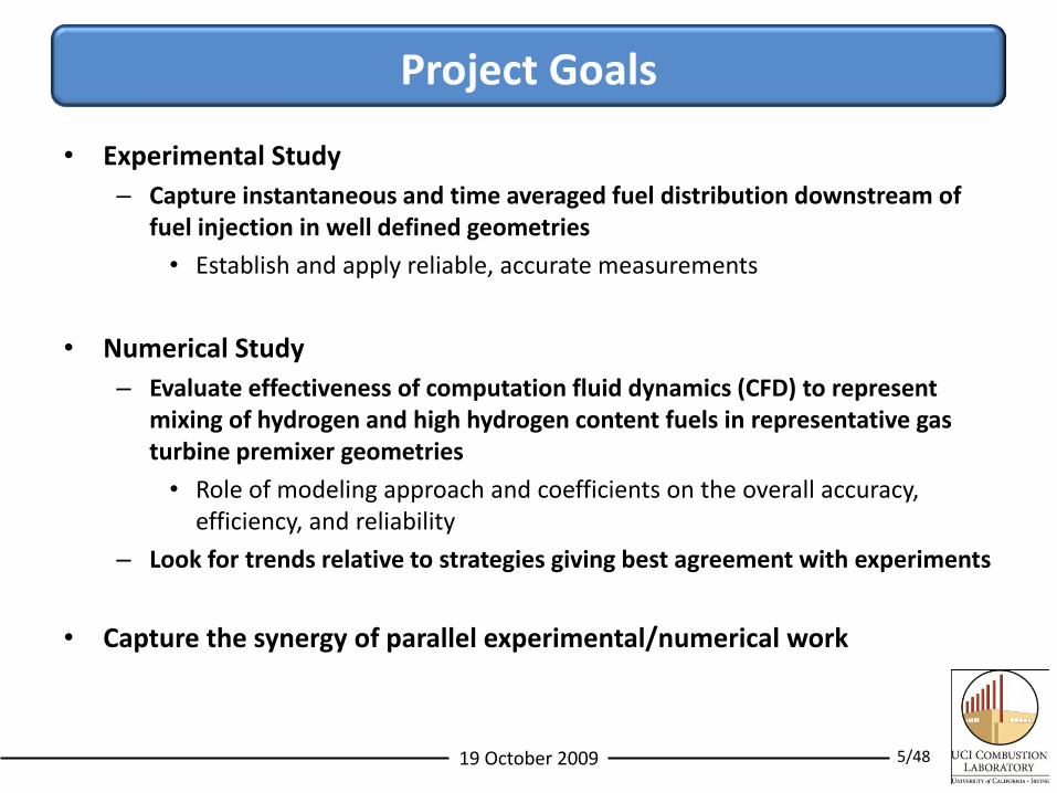
Project Goals
• Experimental Study
– Capture instantaneous and time averaged fuel distribution downstream of fuel injection in well defined geometries
• Establish and apply reliable, accurate measurements
• Numerical Study
– Evaluate effectiveness of computation fluid dynamics (CFD) to represent mixing of hydrogen and high hydrogen content fuels in representative gas turbine premixer geometries
• Role of modeling approach and coefficients on the overall accuracy, efficiency, and reliability
– Look for trends relative to strategies giving best agreement with experiments
• Capture the synergy of parallel experimental/numerical work
19 October 2009 6/48
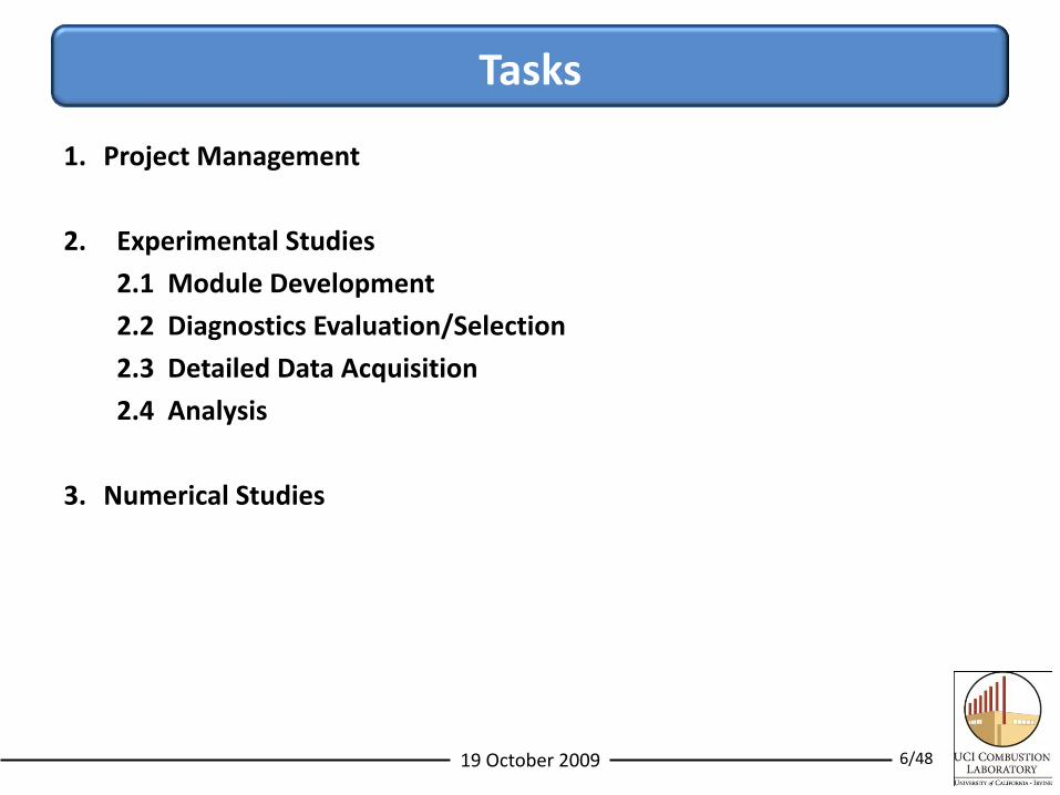
Tasks
1. Project Management
2. Experimental Studies
2.1 Module Development
2.2 Diagnostics Evaluation/Selection
2.3 Detailed Data Acquisition
2.4 Analysis
3. Numerical Studies

19 October 2009 7/48
Tasks
Schedule
Start Date: 1 Oct 2008 contract, 1 Jan 2009 technical startTarget completion date: 31 Dec 2010
19 October 2009 8/48
Task 2 Results
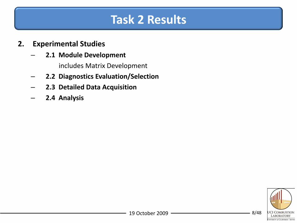
2. Experimental Studies
– 2.1 Module Development
includes Matrix Development
– 2.2 Diagnostics Evaluation/Selection
– 2.3 Detailed Data Acquisition
– 2.4 Analysis
19 October 2009 9/48
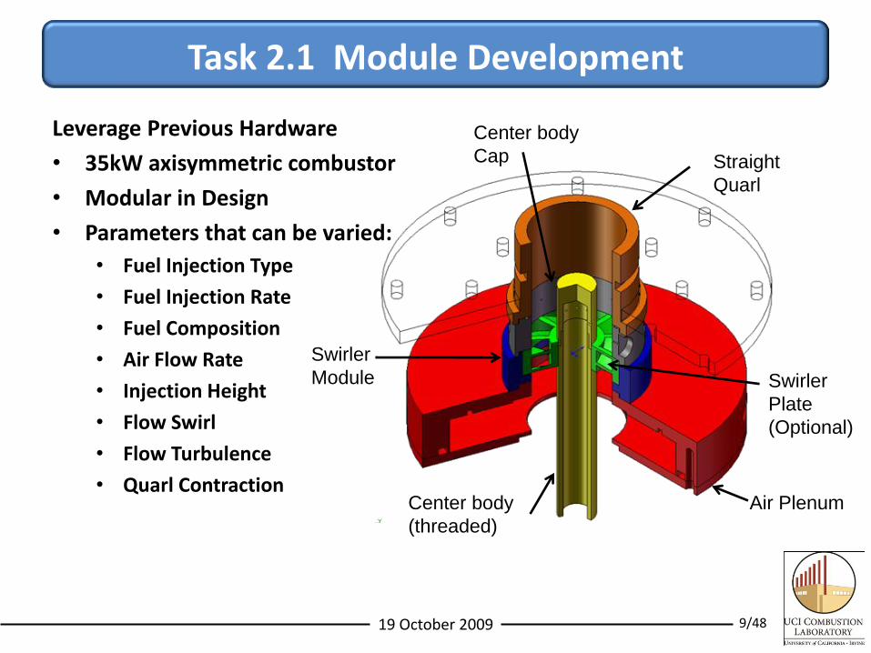
Leverage Previous Hardware
• 35kW axisymmetric combustor
• Modular in Design
• Parameters that can be varied:
• Fuel Injection Type
• Fuel Injection Rate
• Fuel Composition
• Air Flow Rate
• Injection Height
• Flow Swirl
• Flow Turbulence
• Quarl ContractionAir PlenumCenter body
(threaded)
Swirler
Module Swirler
Plate
(Optional)
Straight
Quarl
Task 2.1 Module Development
Center body
Cap
19 October 2009 10/48
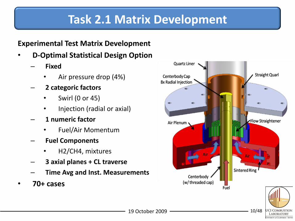
Task 2.1 Matrix Development
Experimental Test Matrix Development
• D-Optimal Statistical Design Option
– Fixed
• Air pressure drop (4%)
– 2 categoric factors
• Swirl (0 or 45)
• Injection (radial or axial)
– 1 numeric factor
• Fuel/Air Momentum
– Fuel Components
• H2/CH4, mixtures
– 3 axial planes + CL traverse
– Time Avg and Inst. Measurements
• 70+ cases
19 October 2009 11/48
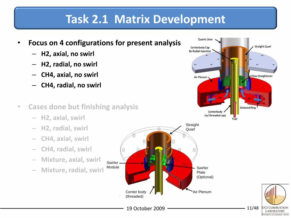
Task 2.1 Matrix Development
• Focus on 4 configurations for present analysis
– H2, axial, no swirl
– H2, radial, no swirl
– CH4, axial, no swirl
– CH4, radial, no swirl
• Cases done but finishing analysis
– H2, axial, swirl
– H2, radial, swirl
– CH4, axial, swirl
– CH4, radial, swirl
– Mixture, axial, swirl
– Mixture, radial, swirl
Air PlenumCenter body
(threaded)
Swirler
Module Swirler
Plate
(Optional)
Straight
Quarl
19 October 2009 12/48
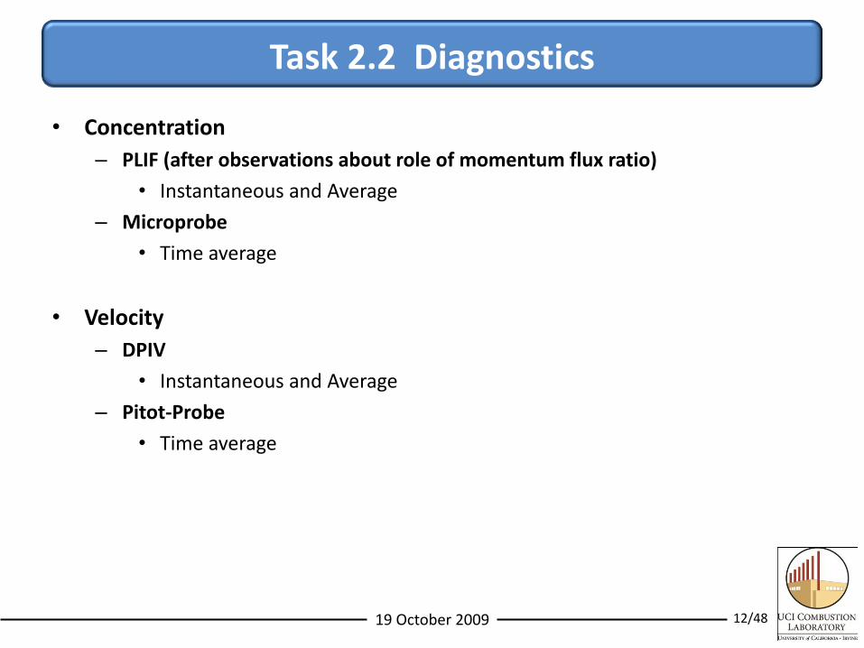
Task 2.2 Diagnostics
• Concentration
– PLIF (after observations about role of momentum flux ratio)
• Instantaneous and Average
– Microprobe
• Time average
• Velocity
– DPIV
• Instantaneous and Average
– Pitot-Probe
• Time average
19 October 2009 13/48
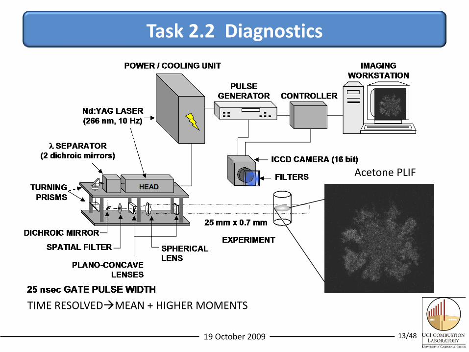
Task 2.2 Diagnostics
Acetone PLIF
TIME RESOLVEDMEAN + HIGHER MOMENTS
19 October 2009 14/48
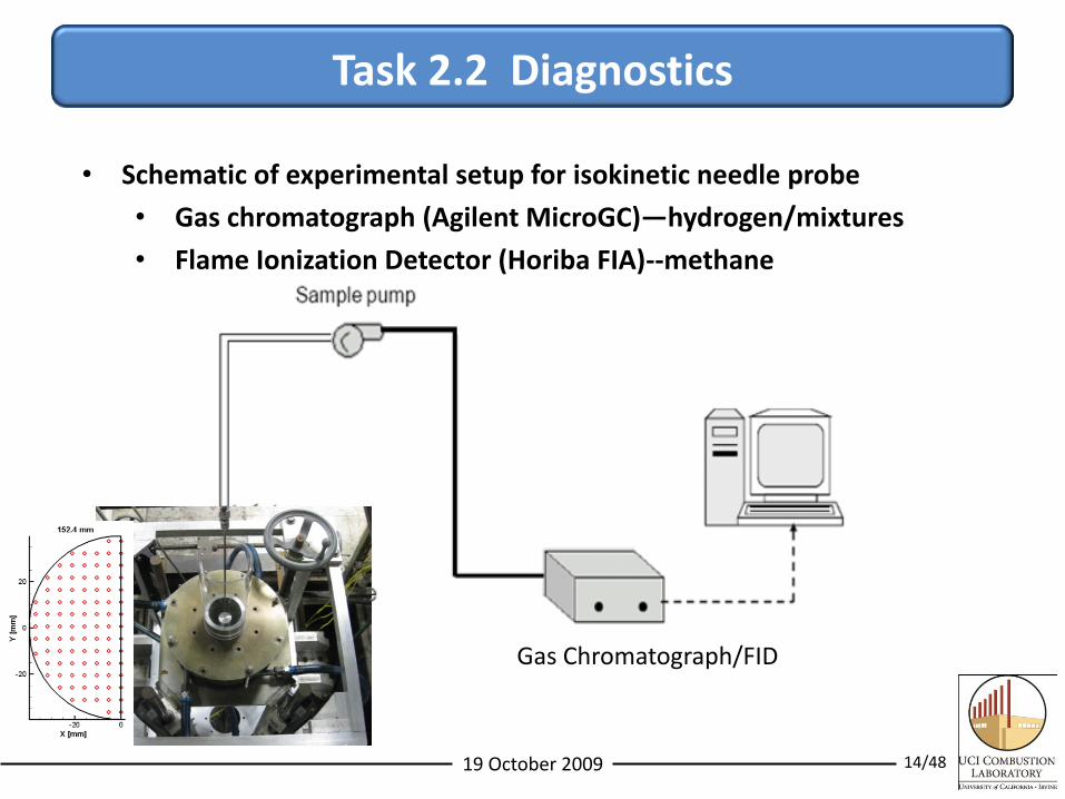
Task 2.2 Diagnostics
• Schematic of experimental setup for isokinetic needle probe
• Gas chromatograph (Agilent MicroGC)—hydrogen/mixtures
• Flame Ionization Detector (Horiba FIA)--methane
Gas Chromatograph/FID
19 October 2009 15/48
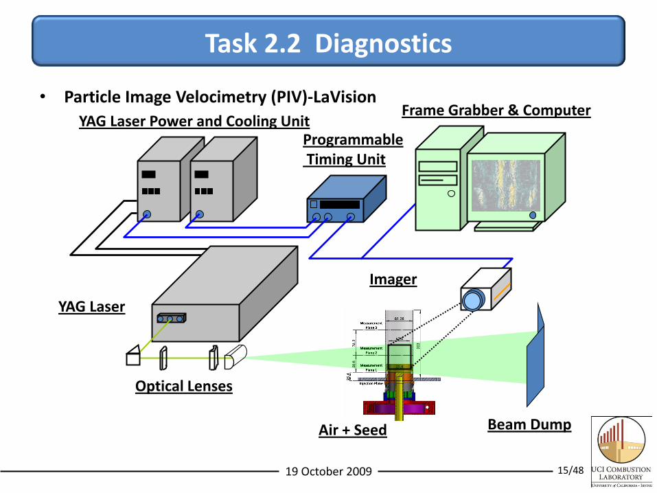
Task 2.2 Diagnostics
• Particle Image Velocimetry (PIV)-LaVision
YAG Laser
ProgrammableTiming Unit
Imager
Frame Grabber & ComputerYAG Laser Power and Cooling Unit
Optical Lenses
Air + Seed Beam Dump
19 October 2009 16/48
Balance of Task 2
• Task 2.3—Data collection—90% complete
• Task 2.4—Analysis—underway
• Will present results in combination with numerical studies
19 October 2009 17/48
Task 3.0 Numerical Studies
Approach
• Computation Fluid Dynamics (CFD) simulations using Fluent
– Common commercial code with collection of models/methods available
• Three major models being evaluated along with key “constants”—emphasis on “near term” tools
– RANS/k-ε model
– RANS/Reynolds Stress Model (RSM)
– URANS
– Large Eddy Simulation
• Objectives Include:
– Finding model coefficients for each modeling strategy to provide accurate predictions of real flows
– Identifying the strengths and weaknesses of the modeling techniques relative to major flow conditions such as the swirl level
19 October 2009 18/48
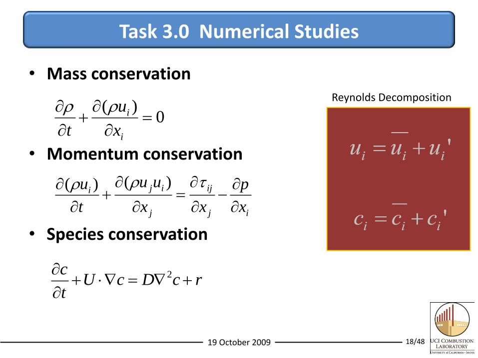
Task 3.0 Numerical Studies
• Mass conservation
• Momentum conservation
• Species conservation
0)(
i
i
x
u
t
ij
ij
j
iji
x
p
xx
uu
t
u
)()(
rcDcUt
c
2
Reynolds Decomposition
19 October 2009 19/48
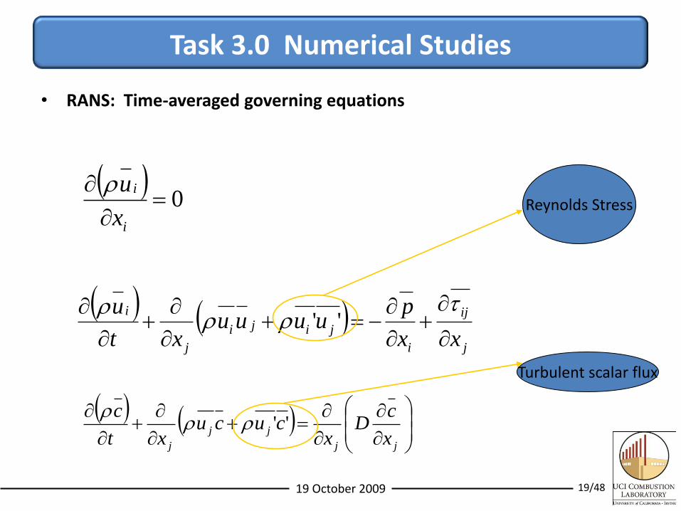
Task 3.0 Numerical Studies
• RANS: Time-averaged governing equations
0
i
i
x
u
j
ij
i
jiji
j
i
xx
puuuu
xt
u
''
jj
jj
j x
cD
xcucu
xt
c''
Reynolds Stress
Turbulent scalar flux
19 October 2009 20/48
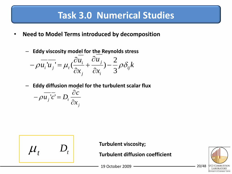
Task 3.0 Numerical Studies
• Need to Model Terms introduced by decomposition
– Eddy viscosity model for the Reynolds stress
– Eddy diffusion model for the turbulent scalar flux
t tD
kx
u
x
uuu ij
i
j
j
itji
3
2)(''
j
tjx
cDcu
''
Turbulent viscosity;
Turbulent diffusion coefficient
19 October 2009 21/48
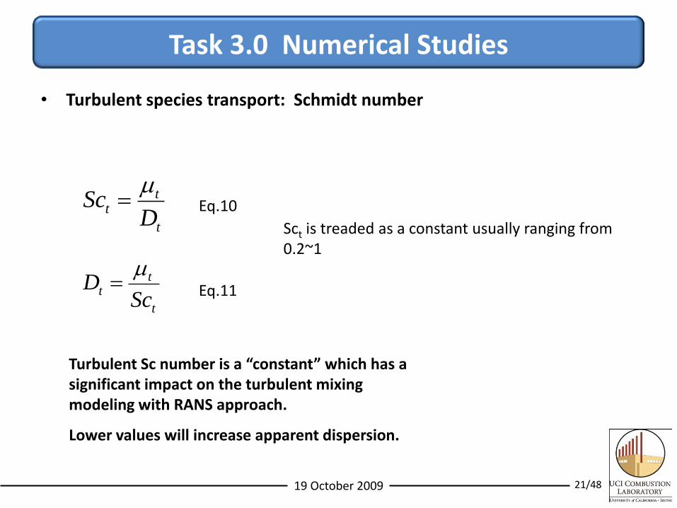
Task 3.0 Numerical Studies
• Turbulent species transport: Schmidt number
t
tt
DSc
t
tt
ScD
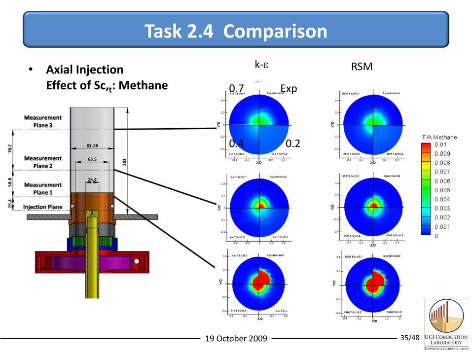
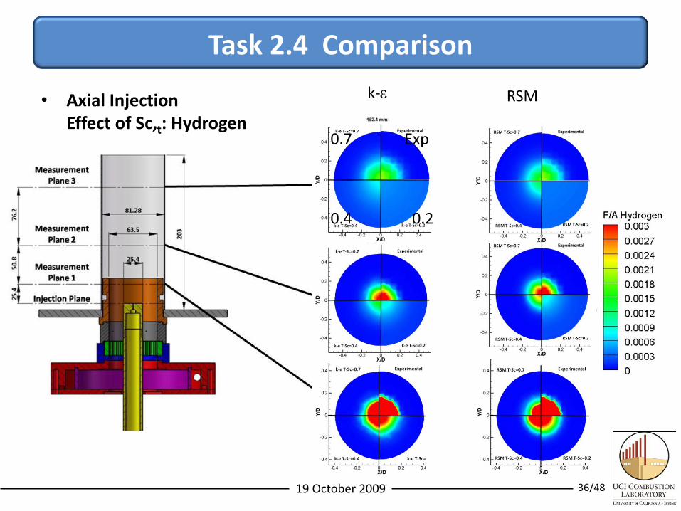
Turbulent Sc number is a “constant” which has a significant impact on the turbulent mixing modeling with RANS approach.
Lower values will increase apparent dispersion.
Sct is treaded as a constant usually ranging from 0.2~1
Eq.10
Eq.11
19 October 2009 22/48
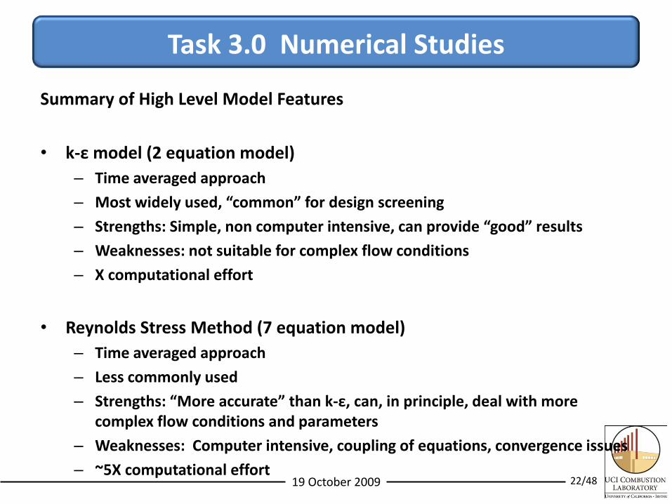
Task 3.0 Numerical Studies
Summary of High Level Model Features
• k-ε model (2 equation model)
– Time averaged approach
– Most widely used, “common” for design screening
– Strengths: Simple, non computer intensive, can provide “good” results
– Weaknesses: not suitable for complex flow conditions
– X computational effort
• Reynolds Stress Method (7 equation model)
– Time averaged approach
– Less commonly used
– Strengths: “More accurate” than k-ε, can, in principle, deal with more complex flow conditions and parameters
– Weaknesses: Computer intensive, coupling of equations, convergence issues
– ~5X computational effort
19 October 2009 23/48
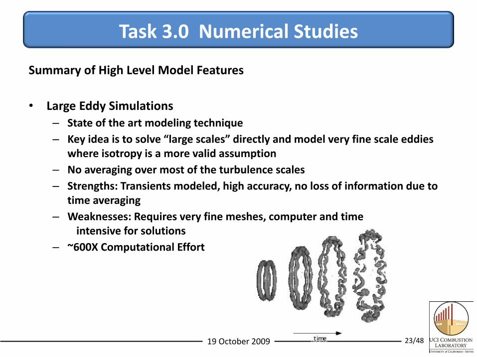
Task 3.0 Numerical Studies
Summary of High Level Model Features
• Large Eddy Simulations
– State of the art modeling technique
– Key idea is to solve “large scales” directly and model very fine scale eddies where isotropy is a more valid assumption
– No averaging over most of the turbulence scales
– Strengths: Transients modeled, high accuracy, no loss of information due to time averaging
– Weaknesses: Requires very fine meshes, computer and time intensive for solutions
– ~600X Computational Effort
19 October 2009 24/48
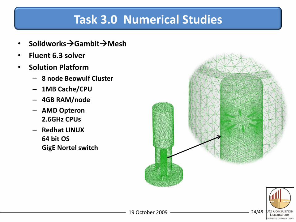
Task 3.0 Numerical Studies
• SolidworksGambitMesh
• Fluent 6.3 solver
• Solution Platform
– 8 node Beowulf Cluster
– 1MB Cache/CPU
– 4GB RAM/node
– AMD Opteron2.6GHz CPUs
– Redhat LINUX64 bit OSGigE Nortel switch
19 October 2009 25/48
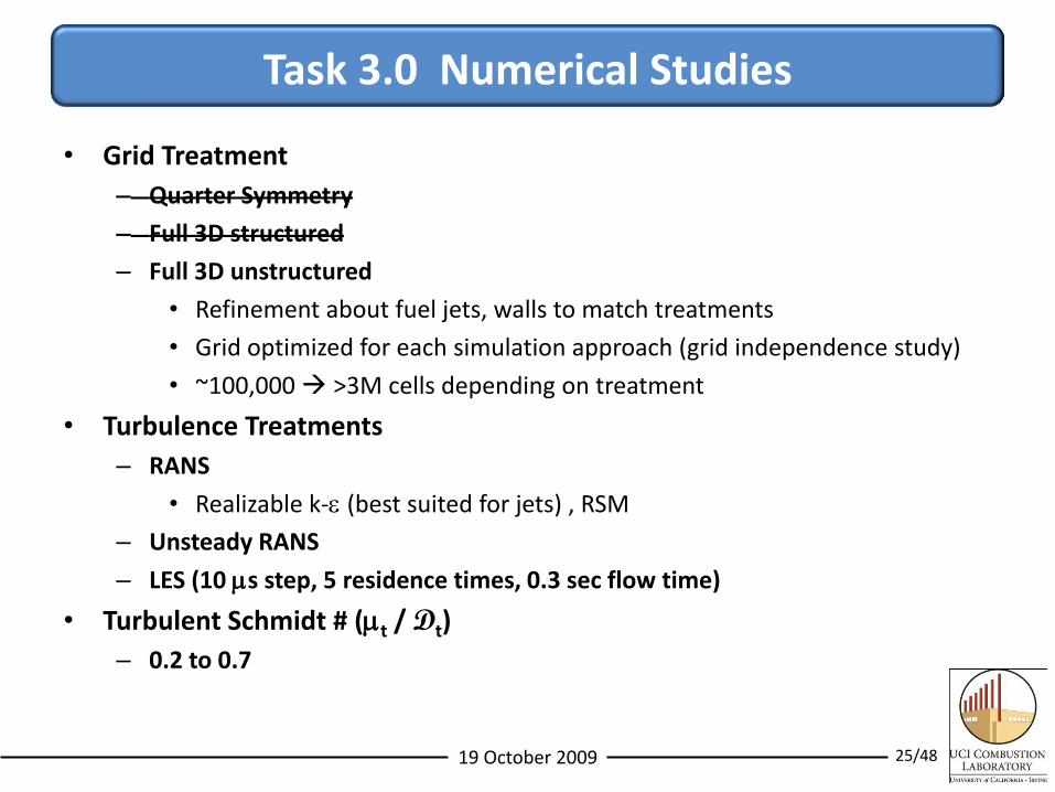
Task 3.0 Numerical Studies
• Grid Treatment
– Quarter Symmetry
– Full 3D structured
– Full 3D unstructured
• Refinement about fuel jets, walls to match treatments
• Grid optimized for each simulation approach (grid independence study)
• ~100,000 >3M cells depending on treatment
• Turbulence Treatments
– RANS
• Realizable k-e (best suited for jets) , RSM
– Unsteady RANS
– LES (10 s step, 5 residence times, 0.3 sec flow time)
• Turbulent Schmidt # (t / Dt)
– 0.2 to 0.7
19 October 2009 26/48
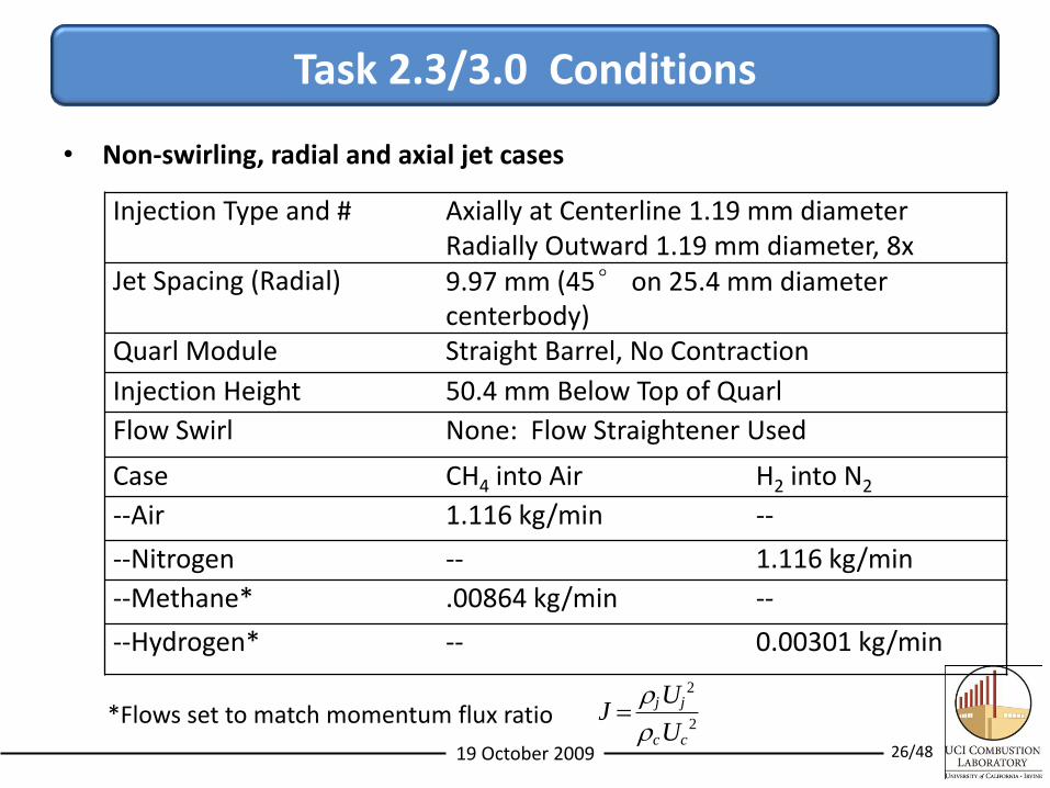
Task 2.3/3.0 Conditions
• Non-swirling, radial and axial jet cases
Injection Type and # Axially at Centerline 1.19 mm diameterRadially Outward 1.19 mm diameter, 8x
Jet Spacing (Radial) 9.97 mm (45° on 25.4 mm diameter centerbody)
Quarl Module Straight Barrel, No Contraction
Injection Height 50.4 mm Below Top of Quarl
Flow Swirl None: Flow Straightener Used
Case CH4 into Air H2 into N2
--Air 1.116 kg/min --
--Nitrogen -- 1.116 kg/min
--Methane* .00864 kg/min --
--Hydrogen* -- 0.00301 kg/min
*Flows set to match momentum flux ratio 2
2
cc
jj
U
UJ
19 October 2009 27/48
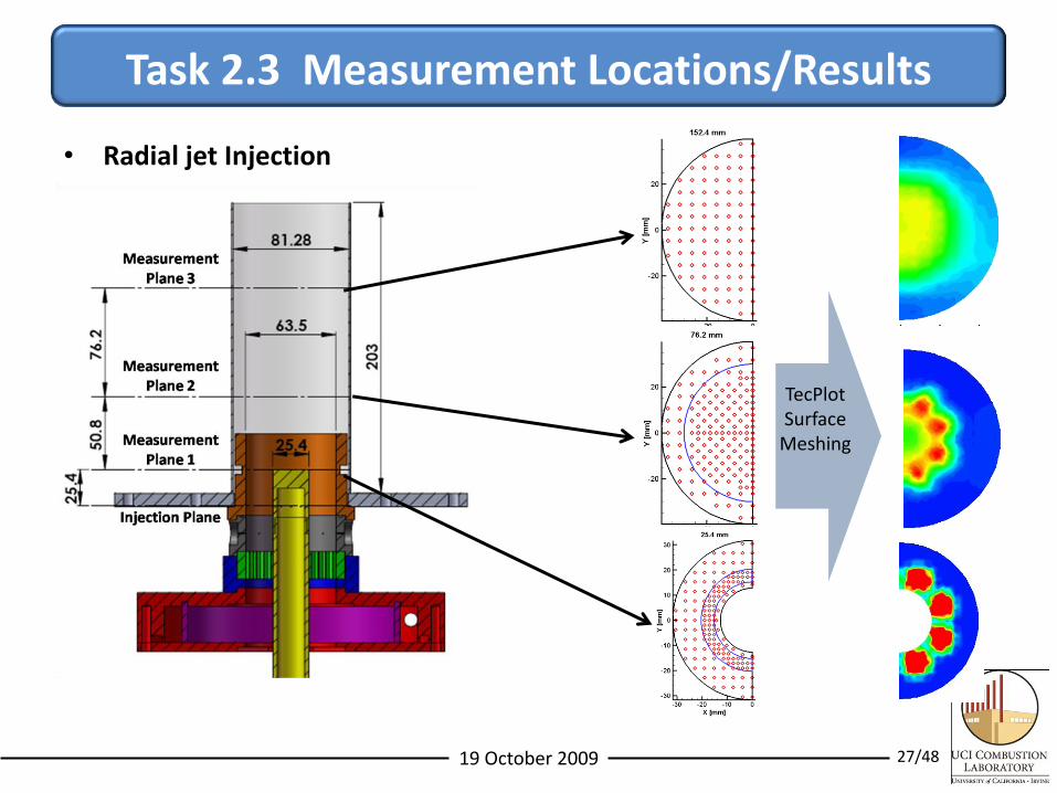
Task 2.3 Measurement Locations/Results
• Radial jet Injection
TecPlotSurface
Meshing
19 October 2009 28/48
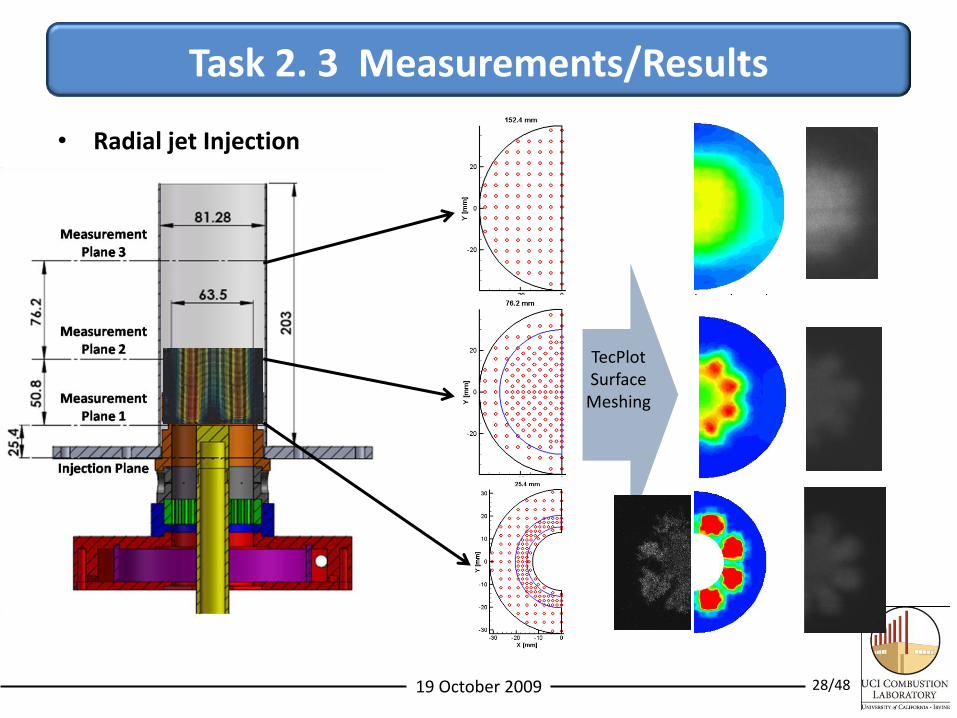
Task 2. 3 Measurements/Results
TecPlotSurface
Meshing
• Radial jet Injection
19 October 2009 29/48
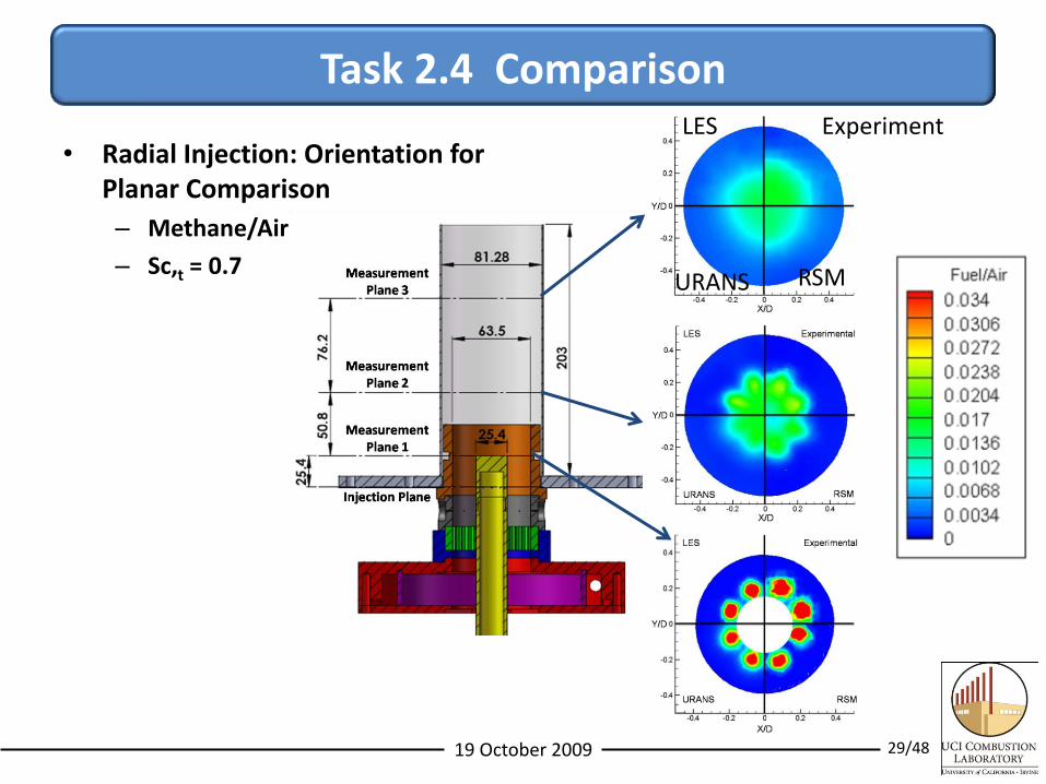
Task 2.4 Comparison
• Radial Injection: Orientation forPlanar Comparison
– Methane/Air
– Sc,t = 0.7
LES Experiment
URANS RSM
19 October 2009 30/48
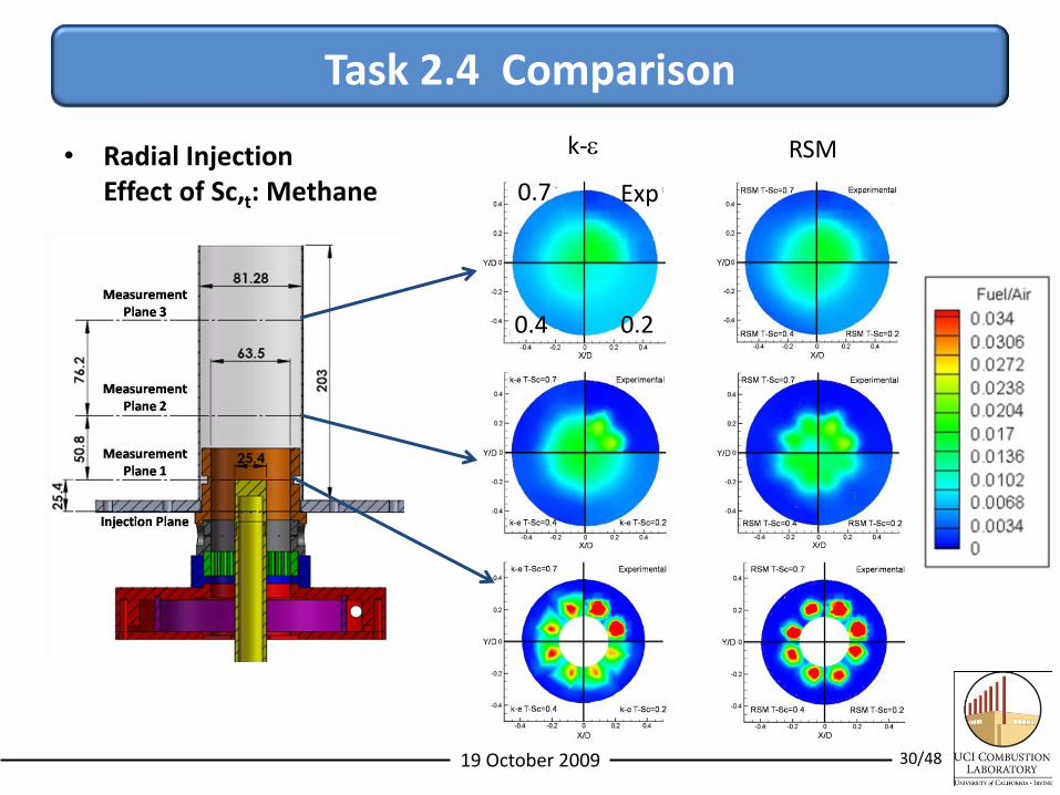
Task 2.4 Comparison
• Radial InjectionEffect of Sc,t: Methane 0.7
0.4 0.2
Exp
k-e RSM
19 October 2009 31/48
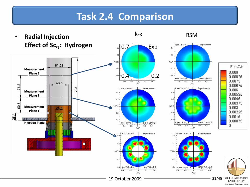
Task 2.4 Comparison
• Radial Injection Effect of Sc,t: Hydrogen
RSM
0.7
0.4 0.2
Exp
k-e
19 October 2009 32/48
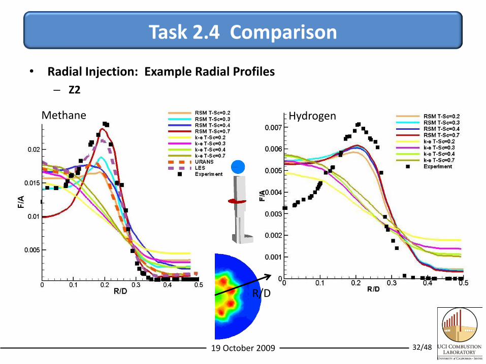
Task 2.4 Comparison
• Radial Injection: Example Radial Profiles
– Z2
Methane Hydrogen
R/D
19 October 2009 33/48
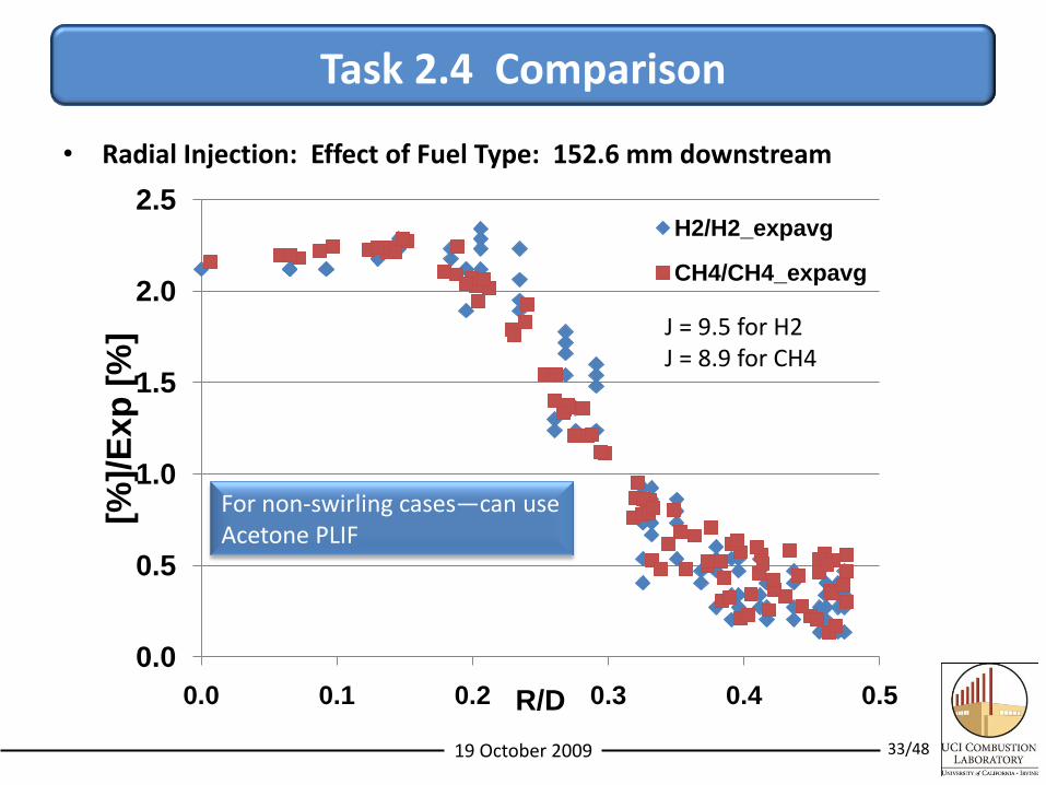
Task 2.4 Comparison
• Radial Injection: Effect of Fuel Type: 152.6 mm downstream
0.0
0.5
1.0
1.5
2.0
2.5
0.0 0.1 0.2 0.3 0.4 0.5
[%]/
Exp
[%
]
R/D
H2/H2_expavg
CH4/CH4_expavg
For non-swirling cases—can useAcetone PLIF
J = 9.5 for H2J = 8.9 for CH4
19 October 2009 34/48
Task 2.4 Comparison
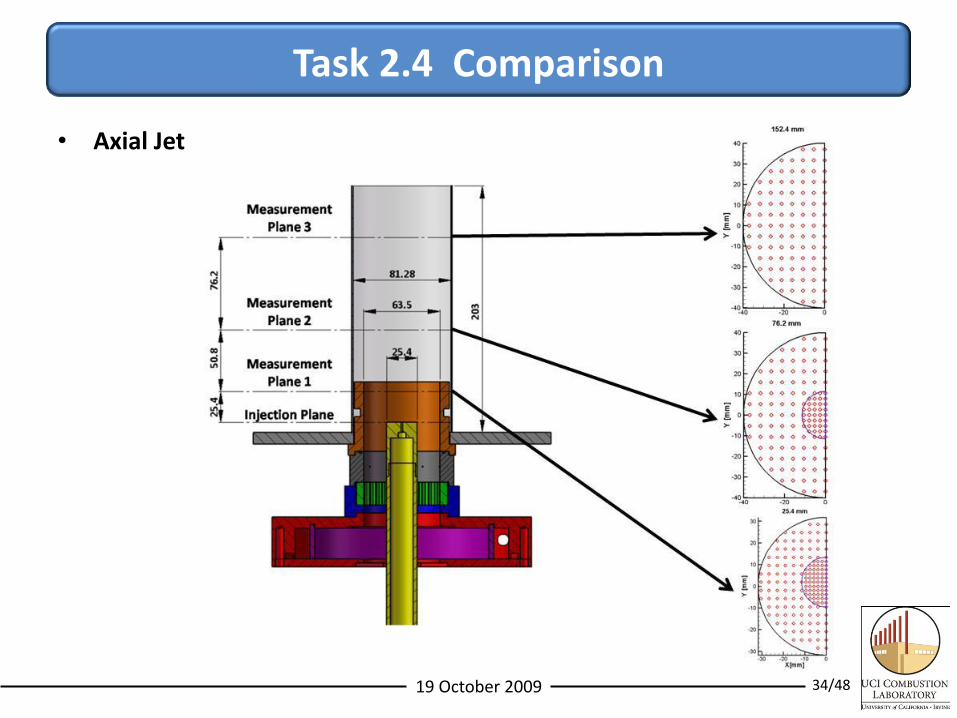
• Axial Jet
19 October 2009 35/48
Task 2.4 Comparison
• Axial InjectionEffect of Sc,t: Methane
RSM
0.7
0.4 0.2
Exp
k-e
19 October 2009 36/48
Task 2.4 Comparison
• Axial InjectionEffect of Sc,t: Hydrogen
RSMk-e
0.7
0.4 0.2
Exp
19 October 2009 37/48
H2CH4
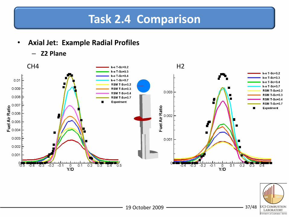
Task 2.4 Comparison
• Axial Jet: Example Radial Profiles
– Z2 Plane
19 October 2009 38/48
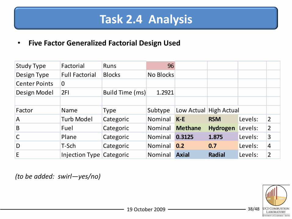
Task 2.4 Analysis
• Five Factor Generalized Factorial Design Used
Study Type Factorial Runs 96
Design Type Full Factorial Blocks No Blocks
Center Points 0
Design Model 2FI Build Time (ms) 1.2921
Factor Name Type Subtype Low Actual High Actual
A Turb Model Categoric Nominal K-E RSM Levels: 2
B Fuel Categoric Nominal Methane Hydrogen Levels: 2
C Plane Categoric Nominal 0.3125 1.875 Levels: 3
D T-Sch Categoric Nominal 0.2 0.7 Levels: 4
E Injection Type Categoric Nominal Axial Radial Levels: 2
(to be added: swirl—yes/no)
19 October 2009 39/48
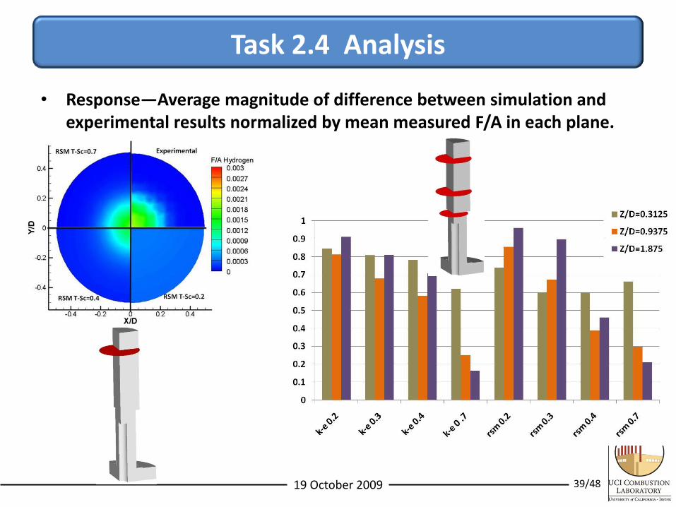
Figure 1- normalized averaged fuel/air differences between experiment and
numerical cases over the planes (methane) for axial injection configuration
Task 2.4 Analysis
• Response—Average magnitude of difference between simulation and experimental results normalized by mean measured F/A in each plane.
19 October 2009 40/48
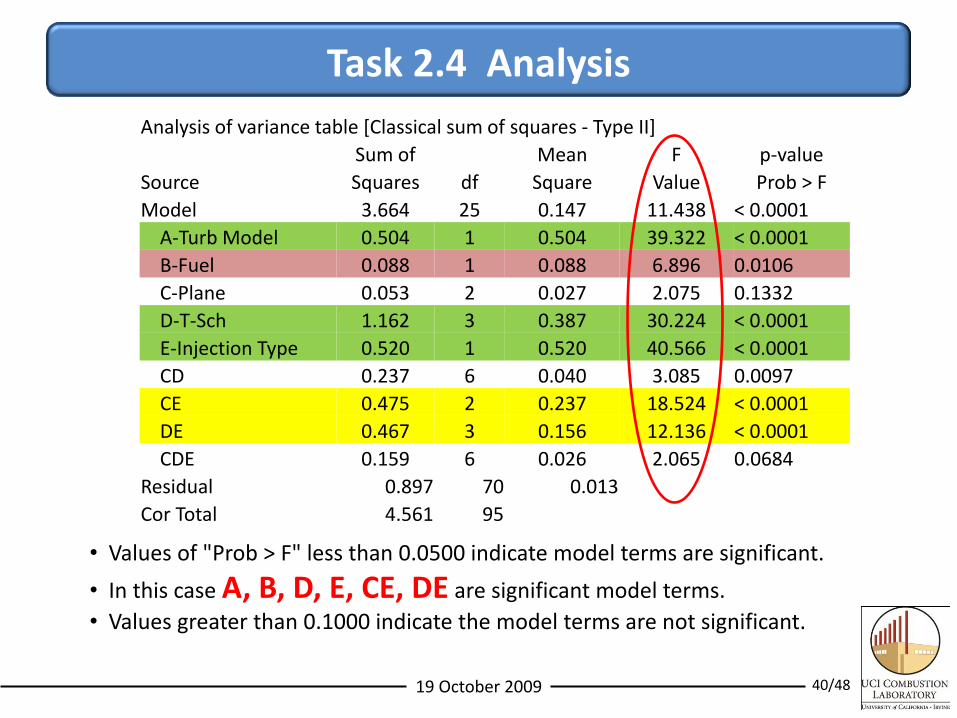
Analysis of variance table [Classical sum of squares - Type II]
Sum of Mean F p-value
Source Squares df Square Value Prob > F
Model 3.664 25 0.147 11.438 < 0.0001
A-Turb Model 0.504 1 0.504 39.322 < 0.0001
B-Fuel 0.088 1 0.088 6.896 0.0106
C-Plane 0.053 2 0.027 2.075 0.1332
D-T-Sch 1.162 3 0.387 30.224 < 0.0001
E-Injection Type 0.520 1 0.520 40.566 < 0.0001
CD 0.237 6 0.040 3.085 0.0097
CE 0.475 2 0.237 18.524 < 0.0001
DE 0.467 3 0.156 12.136 < 0.0001
CDE 0.159 6 0.026 2.065 0.0684
Residual 0.897 70 0.013
Cor Total 4.561 95
• Values of "Prob > F" less than 0.0500 indicate model terms are significant.
• In this case A, B, D, E, CE, DE are significant model terms.
• Values greater than 0.1000 indicate the model terms are not significant.
Task 2.4 Analysis
19 October 2009 41/48
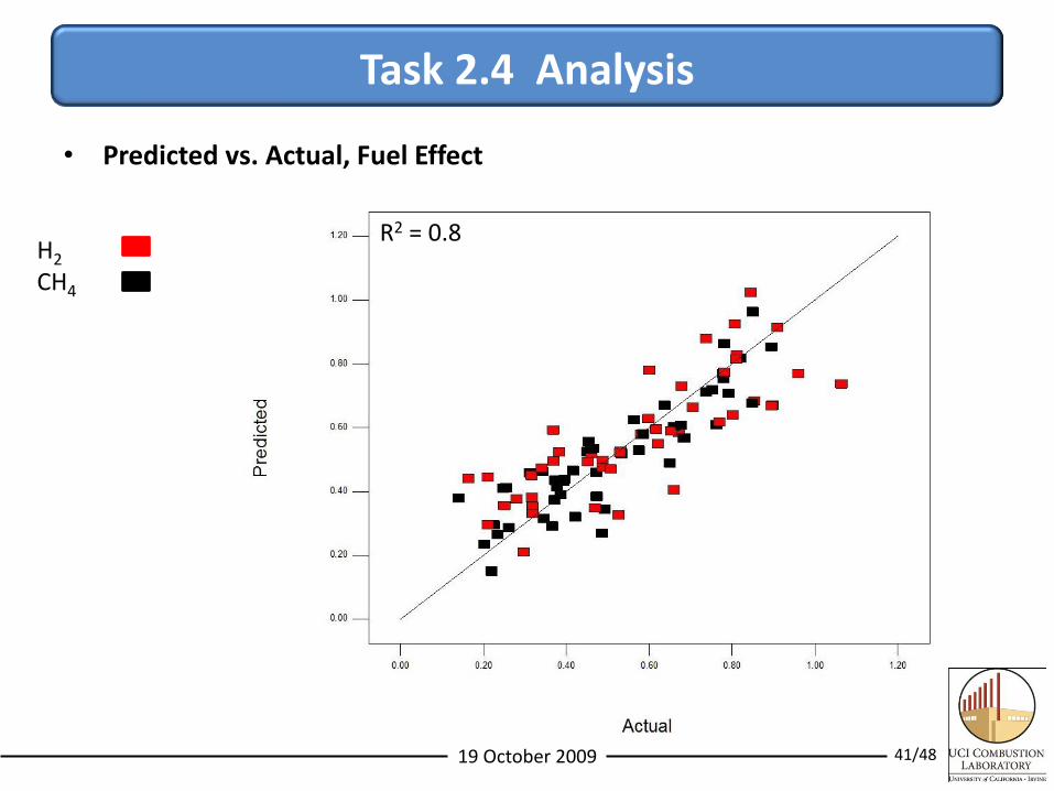
Task 2.4 Analysis
• Predicted vs. Actual, Fuel Effect
H2
CH4
R2 = 0.8
19 October 2009 42/48
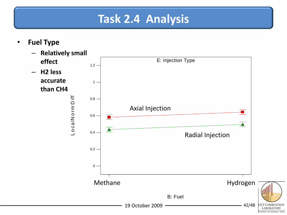
Design-Expert® Software
LocalNormDiff
X1 = B: Fuel
X2 = E: Injection Type
Actual Factors
A: Turb Model = Average
C: Plane = Average
D: T-Sch = Average
E1 Axial
E2 Radial
E: Injection Type
Methane Hydrogen
Interaction
B: Fuel
Lo
ca
lNo
rmD
iff
0
0.2
0.4
0.6
0.8
1
1.2
Task 2.4 Analysis
• Fuel Type
– Relatively smalleffect
– H2 lessaccuratethan CH4
Axial Injection
Radial Injection
Methane Hydrogen
19 October 2009 43/48
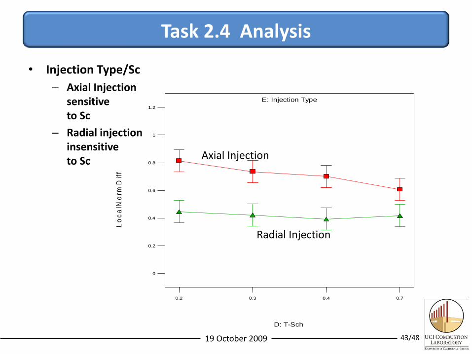
Design-Expert® Software
LocalNormDiff
X1 = D: T-Sch
X2 = E: Injection Type
Actual Factors
A: Turb Model = Average
B: Fuel = Average
C: Plane = 0.3125
E1 Axial
E2 Radial
E: Injection Type
0.2 0.3 0.4 0.7
Interaction
D: T-Sch
Lo
ca
lNo
rmD
iff
0
0.2
0.4
0.6
0.8
1
1.2
Axial Injection
Radial Injection
Task 2.4 Analysis
• Injection Type/Sc
– Axial Injectionsensitiveto Sc
– Radial injectioninsensitiveto Sc
19 October 2009 44/48
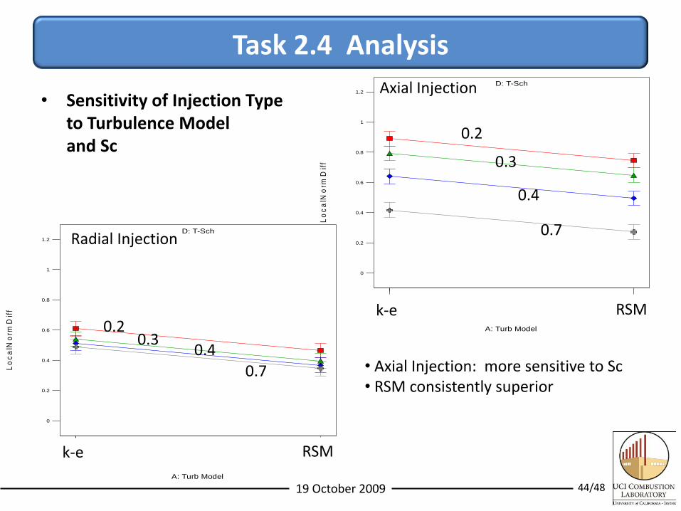
Design-Expert® Software
LocalNormDiff
X1 = A: Turb Model
X2 = D: T-Sch
Actual Factors
B: Fuel = Average
C: Plane = Average
E: Injection Type = Axial
D1 0.2
D2 0.3
D3 0.4
D4 0.7
D: T-Sch
K-E RSM
Interaction
A: Turb ModelL
oc
alN
orm
Dif
f
0
0.2
0.4
0.6
0.8
1
1.2 Axial Injection
Design-Expert® Software
LocalNormDiff
X1 = A: Turb Model
X2 = D: T-Sch
Actual Factors
B: Fuel = Average
C: Plane = Average
E: Injection Type = Radial
D1 0.2
D2 0.3
D3 0.4
D4 0.7
D: T-Sch
K-E RSM
Interaction
A: Turb Model
Lo
ca
lNo
rmD
iff
0
0.2
0.4
0.6
0.8
1
1.2 Radial Injection
Task 2.4 Analysis
• Sensitivity of Injection Typeto Turbulence Modeland Sc
• Axial Injection: more sensitive to Sc• RSM consistently superior
0.7
0.4
0.3
0.2
0.70.4
0.30.2
k-e RSM
k-e RSM
19 October 2009 45/48
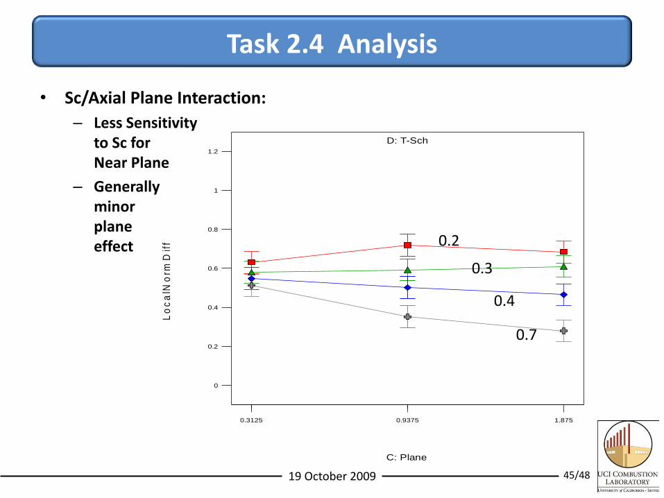
Design-Expert® Software
LocalNormDiff
X1 = C: Plane
X2 = D: T-Sch
Actual Factors
A: Turb Model = Average
B: Fuel = Average
E: Injection Type = Average
D1 0.2
D2 0.3
D3 0.4
D4 0.7
D: T-Sch
0.3125 0.9375 1.875
Interaction
C: Plane
Lo
ca
lNo
rmD
iff
0
0.2
0.4
0.6
0.8
1
1.2
Task 2.4 Analysis
• Sc/Axial Plane Interaction:
– Less Sensitivityto Sc for Near Plane
– Generallyminorplaneeffect
0.7
0.4
0.3
0.2
19 October 2009 46/48
Axial Injection
Radial Injection
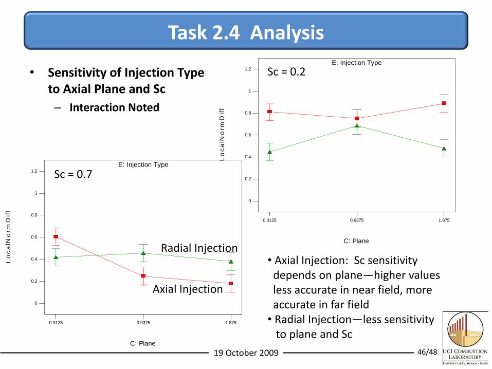
Task 2.4 Analysis
• Sensitivity of Injection Typeto Axial Plane and Sc
– Interaction Noted
• Axial Injection: Sc sensitivitydepends on plane—higher valuesless accurate in near field, moreaccurate in far field
• Radial Injection—less sensitivityto plane and Sc
Design-Expert® Software
LocalNormDiff
X1 = C: Plane
X2 = E: Injection Type
Actual Factors
A: Turb Model = Average
B: Fuel = Average
D: T-Sch = 0.2
E1 Axial
E2 Radial
E: Injection Type
0.3125 0.9375 1.875
Interaction
C: Plane
Lo
ca
lNo
rmD
iff
0
0.2
0.4
0.6
0.8
1
1.2
Design-Expert® Software
LocalNormDiff
X1 = C: Plane
X2 = E: Injection Type
Actual Factors
A: Turb Model = Average
B: Fuel = Average
D: T-Sch = 0.7
E1 Axial
E2 Radial
E: Injection Type
0.3125 0.9375 1.875
Interaction
C: Plane
Lo
ca
lNo
rmD
iff
0
0.2
0.4
0.6
0.8
1
1.2 Sc = 0.7
Sc = 0.2
19 October 2009 47/48
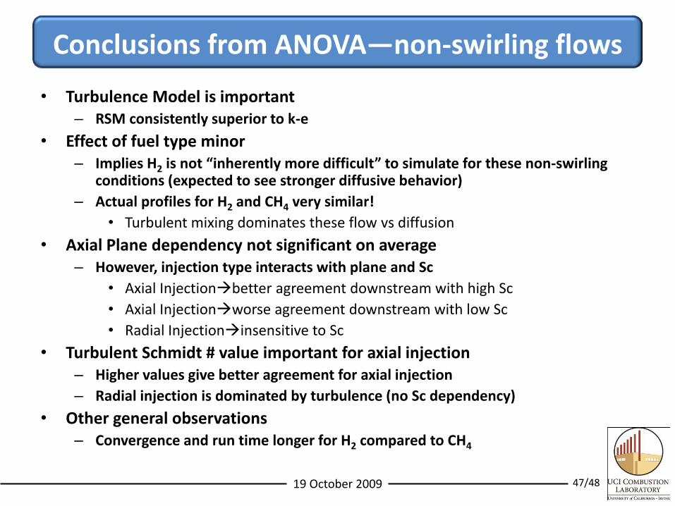
Conclusions from ANOVA—non-swirling flows
• Turbulence Model is important– RSM consistently superior to k-e
• Effect of fuel type minor– Implies H2 is not “inherently more difficult” to simulate for these non-swirling
conditions (expected to see stronger diffusive behavior)
– Actual profiles for H2 and CH4 very similar!
• Turbulent mixing dominates these flow vs diffusion
• Axial Plane dependency not significant on average– However, injection type interacts with plane and Sc
• Axial Injectionbetter agreement downstream with high Sc
• Axial Injectionworse agreement downstream with low Sc
• Radial Injectioninsensitive to Sc
• Turbulent Schmidt # value important for axial injection– Higher values give better agreement for axial injection
– Radial injection is dominated by turbulence (no Sc dependency)
• Other general observations– Convergence and run time longer for H2 compared to CH4
19 October 2009 48/48
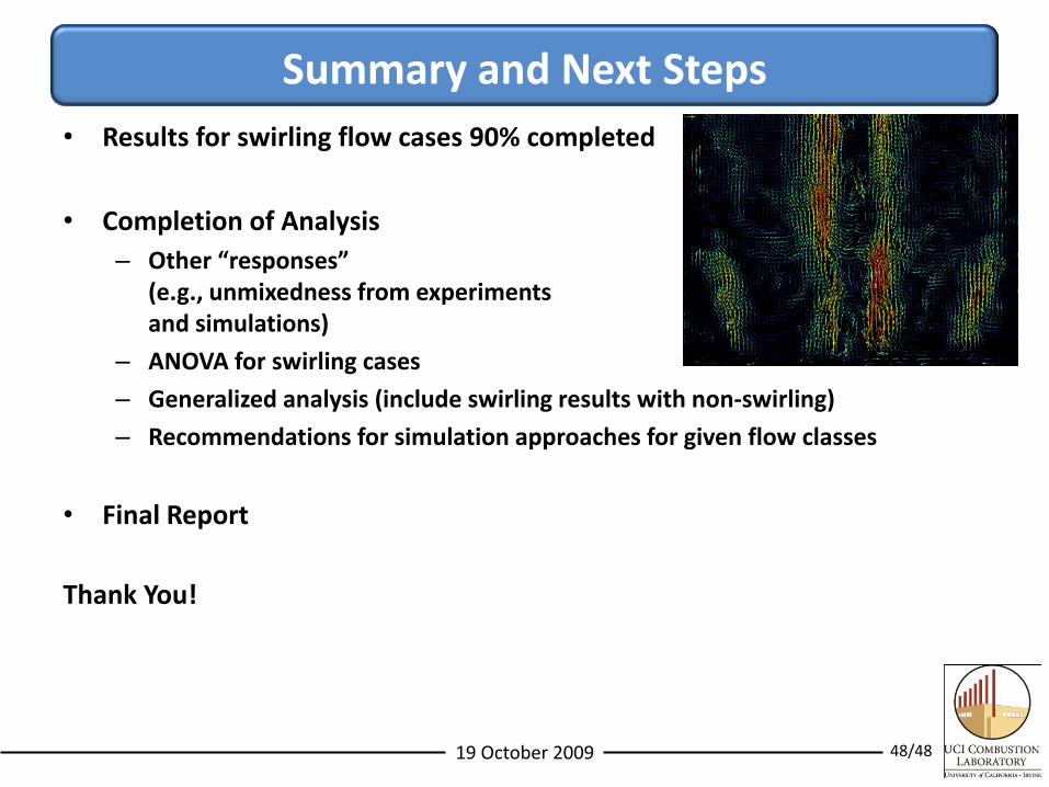
Summary and Next Steps
• Results for swirling flow cases 90% completed
• Completion of Analysis
– Other “responses” (e.g., unmixedness from experiments and simulations)
– ANOVA for swirling cases
– Generalized analysis (include swirling results with non-swirling)
– Recommendations for simulation approaches for given flow classes
• Final Report
Thank You!