Embed Size (px)
Citation preview

Numerical Simulation of Nanoscale Flow:
A Molecular Dynamics Study of Drag
By
Tim Sirk
Thesis submitted to the faculty of the
Virginia Polytechnic Institute and State University
in partial fulfillment of the requirements for the degree of
Master of Science
in
Mechanical Engineering
Dr. Eugene Brown, Chairman Mechanical Engineering
Dr. Mark Paul Dr. Eugene Cliff Mechanical Engineering Aerospace Engineering
April 28, 2006 Blacksburg, VA
Keywords: Nano, Drag, Sphere, Biosensor Copyright 2006, Tim Sirk

Numerical Simulation of Nanoscale Flow:
A Molecular Dynamics Study of Drag
By
Tim Sirk
(ABSTRACT)
The design of pathogen biosensors may soon incorporate beads having a
nanoscale diameter, thus making the drag force on a nanoscale sphere an important
engineering problem. Flows at this small of a scale begin to appear “grainy” and may not
always behave as a continuous fluid. Molecular dynamics provides an approach to
determine drag forces in those nanoscale flows which cannot be described with
continuum (Navier-Stokes) theory.
This thesis uses a molecular dynamics approach to find the drag forces acting on a
sphere and a wall under several different conditions. The results are compared with
approximations from a Navier-Stokes treatment and found to be within an order of
magnitude despite the uncertainties involved in both the atomic interactions of the
molecular dynamics simulation and the appropriate boundary conditions in the Navier-
Stokes solution.

iii
Acknowledgements
I would like to thank the faculty of the Interdisciplinary Center for Applied
Mathematics at Virginia Tech for the use of their SGI Origin 2000 as well as the staff of
the Computational Physics & Fluid Dynamics Division of the Naval Research Laboratory
(NRL) for the use of their SGI Origin 3200. A special thanks to Bill Sandberg for his
insight and suggestions during my stay at NRL.
I would like to express my gratitude to Dr. Eugene Brown for his guidance during
the course of this research. Our many conversations regarding thermodynamics and fluid
dynamics have been very insightful. Dr. Eugene Cliff and Dr. Mark Paul have also been
great resources and were kind of enough to serve as members of my committee. A
special thanks to Dr. Zhigang Li for sharing his experiences modeling drag force with
molecular dynamics.
A final thanks to my wife, Hanh Vu, for her support and newfound appreciation
of atoms.
The first principle is that you must not fool yourself - and you are the easiest
person to fool.
-Richard Feynman

iv
Table of Contents
Chapter 1: Introduction to Molecular Dynamics............................................................... 1
1.1 Motivation ................................................................................................................. 1
1.2 Common Uses of Molecular Dynamics in Fluid Mechanics..................................... 1
1.3 Foundations of Molecular Dynamics........................................................................ 4
1.4 The Scope of Molecular Dynamics............................................................................ 6
1.4.1 Classical Forces .......................................................................................... 7
1.4.2 Computational Power.................................................................................. 7
1.5 Potential Energy Models........................................................................................... 8
1.6 Potential Energy Truncation and Long-Range Corrections ................................... 11
1.7 Periodic boundary conditions ................................................................................. 12
1.8 Time integration algorithms.................................................................................... 13
Chapter 2: Literature Review........................................................................................... 16
2.1 Historical Background ............................................................................................ 16
2.2 Poiseuille Flow........................................................................................................ 18
2.3 Drag Force and Stokes Law.................................................................................... 21
2.4 Wall Models............................................................................................................ 23
2.5 Comprehensive References ..................................................................................... 25
Chapter 3: LAMMPS and Visualization Software ........................................................... 26
3.1 LAMMPS – Large Atomic Molecular Massively Parallel Simulator ................. 26
3.2 LAMMPS Operation ........................................................................................... 27
3.3 LAMMPS Pre- and Postprocessing .................................................................... 28
3.4 Visual Molecular Dynamics................................................................................ 29
Chapter 4: Development of Biosensor Inspired Problems............................................... 31
Chapter 5: Validation of the LAMMPS Code .................................................................. 33
5.1 The Need for a Validation Problem .................................................................... 33
5.2 Modeling Considerations.................................................................................... 33
5.3 Equilibration of the System ................................................................................ 34
5.4 NEMD Simulation ............................................................................................... 38
5.5 Validation Results ............................................................................................... 40
Chapter 6: Setup of the Research Runs............................................................................ 42
6.1 Similarities with the Validation Case.................................................................. 42
6.2 The Modeling of the Wall................................................................................... 42
6.3 Sizing the Simulation Box .................................................................................. 44
6.4 Comparing with Continuum Results ................................................................... 46
Chapter 7: Results of the Research Runs ........................................................................ 47
7.1 Problem 1: Drag on an Isolated Sphere ............................................................ 47
7.2 Problem 2: Friction on a Wall ........................................................................... 50
7.3 Problem 3: Drag on a Sphere near a Wall ......................................................... 53
Chapter 8: Suggestions for Future Work ........................................................................ 56
Appendix............................................................................................................................ 58
References ......................................................................................................................... 61
Vita .................................................................................................................................... 63

v
Table of Figures
Figure 1.1. Modeling methods in discrete and continuum regions.................................... 2
Figure 1.2. Components of the Lennard-Jones Potential ................................................ 10
Figure 1.3. Periodic boundary conditions ........................................................................ 13
Figure 2.1. The velocity profile of a small channel ......................................................... 20
Figure 2.2. The velocity profile of larger channel ........................................................... 20
Figure 2.3. Examples of wake oscillations....................................................................... 21
Figure 2.4. Density gradients........................................................................................... 23
Figure 3.1. VMD interface. .............................................................................................. 30
Figure 5.1. The fluidic system before equilibration ......................................................... 35
Figure 5.2. Maxwell distribution...................................................................................... 36
Figure 5.3 Repulsive force fields...................................................................................... 38
Figure 5.4. Geometry of the validation problem.............................................................. 39
Figure 5.5. Approach to steady-state drag ...................................................................... 40
Figure 6.1. The atomic wall ............................................................................................. 43
Figure 7.1. Drag coefficient of a nanosphere .................................................................. 48
Figure 7.2. Drag force as a function of Re from MD and Navier-Stokes ......................... 49
Figure 7.3. Position and motion of the wall..................................................................... 50
Figure 7.4. Response of drag coefficient to number density of a wall............................. 51
Figure 7.5. Drag coefficient as a function of wall seperation .......................................... 54
Figure A.1. Number of accessible states .......................................................................... 60

1
Chapter 1: Introduction to Molecular Dynamics
1.1 Motivation
A renewed interest in detecting chemical and biological agents has encouraged
researchers to improve old biosensor designs as well as develop new ones. Two
microbead-type biosensors under development at the Chemistry Division of the Naval
Research Laboratory are the Bead Array Counter (BARC) and Force Discrimination
Biosensor (FDB). Downsizing these biosensor designs could be a major step forward in
both sensitivity and analysis time with the added benefit of lab-on-a-chip technology.
A process within both biosensor designs involves removing a number of micron
size beads from a fluid-filled channel using either magnetic or fluidic forces. In the
future, it will be desirable to significantly shrink these beads for the sake of performance,
perhaps down to the nanoscale level. The behavior of these nanobeads would enter a
realm of physics not accessible to continuum fluid dynamics.
The behavior of nanobeads is important to performance, particularly when a bead
moves near a channel wall. The biosensor is designed such that nanobeads either attach
themselves directly to a channel wall or become tethered to the wall by DNA. For best
performance, these designs require an understanding of the flow behavior around
nanosize objects, especially spheres, near and at a channel wall. Gijs provides a more
complete introduction to biosensors [Gijs, 2004].
1.2 Common Uses of Molecular Dynamics in Fluid Mechanics
Classical fluid mechanics assumes fluid motion is governed by the Navier-Stokes
equations. This model has proven quite accurate since its conception and still remains
the dominant model of fluid dynamics. However, recently some systems of interest have

2
become small enough to be modeled discretely on an atomic scale. In these situations, a
purely continuum description of fluid motion is obviously inappropriate.
How a system is to be modeled usually begins by judging the length scale of the
problem. Several important physical models with their corresponding length and time
scales are shown below in Figure 1.1.
Figure 1.1. Modeling methods in discrete and continuum regimes.
Because the diameter an atom is comparable to a characteristic length of the
problem’s geometry, flow systems with dimensions of order 10-9m are best treated as
discrete collections of atoms rather than a continuous fluid. For example, the Navier-
Hour
Microsec
Nanosec
Picosec
Femtosec
Minute
Second
Å nm 10 nm micron mm m
Finite Element Analysis
Mesoscale Dynamics
Molecular Dynamics F = MA
Quantum Mechanics

3
Stokes solutions for Poiseuille flow are typically reliable down to a channel diameter of
10 molecular widths [Travis, 1997]. Beyond this limit other modeling methods must be
used to describe the fluid motion.
Analytical solutions of multi-body problems are usually not practical for any
discrete fluid of a significant volume. Statistical mechanics provides insight into a few
cases with limiting behavior; however, computational methods are available that evaluate
fluid behavior under many more conditions.
Notice in Figure 1.1 that molecular dynamics (MD) is sandwiched between the
infinitesimal world of quantum mechanics and mesoscale dynamics. Many sciences are
able to use a mesoscale model to bridge MD and continuum theory, such as nucleation
modeling in material science. The mesoscale “bridge” serves to save time when the
detailed results of MD are not needed; however, this approach is not always applicable.
Fluids generally do not form mesoscale structures and jump directly from MD to
continuum theory, provided that an acceptable MD model is known. Monte Carlo and
Lattice Boltzmann methods (not shown) overlap both the upper domain of MD and the
lower domain of continuum length scales, but obtaining information concerning the
movement of individual atoms still requires an MD simulation.
Unlike Lattice Boltzmann and Monte Carlo, MD provides a complete description
of fluid behavior by finding the trajectory of each atom or molecule as it moves within a
fluid. Probabilistic input, such as velocity distribution functions, is not part of an MD
model. Unfortunately, an MD approach is computationally expensive and the volume of
fluid that can be modeled remains limited despite advances in computer power [Haile,
1997].
The time consuming process of generating detailed information about each atom
in the fluid does provide MD with one striking advantage: A broad range of problems

4
may be solved in a conceptually straightforward way. As long as the appropriate
interatomic forces can be calculated, any boundary conditions are completely modeled
thus leaving only the number of atoms as the primary factor in deciding which problems
may be solved.
MD simulation typically does not model forces directly from quantum mechanical
effects, instead forming all quantum considerations into classical potential energy
functions. The Lennard-Jones potential is perhaps the most famous of these, although
many exist. Many potentials can accurately describe the behavior of only a few
substances. For example, the Lennard-Jones 12-6 potential is known for its accurate
description of argon gas [Haile, 1997].
Outside of its original use in the simulation of static, or “equilibrium” fluids, MD
is often used in simulations of fluids under a net external force. These “nonequilibrium”
processes involve motion caused by sources other than thermal energy, such as pressure
driven flow in a nano-dimensional channel. Simulation employing these processes is
described as nonequilibrium molecular dynamics (NEMD) [Haile, 1997].
1.3 Foundations of Molecular Dynamics
Some results of statistical mechanics are needed to determine physical properties
of the fluid during the simulation. In this work, as in the majority of other MD fluid
simulations, a closed system with a constant number of atoms, constant volume, and
constant energy is used. All of the possible physical states of a system with this
combination of fixed properties are known as the microcanonical ensemble (NVE).
The temperature of a fluid is evaluated from statistical mechanics (from the
microcanonical ensemble) as
(1.1)

5
where N is the number of particles, kB is Boltzmann’s constant and KE is the kinetic
energy of the system [Haile, 1997]. Kinetic energy is determined as
(1.2)
where mi and vi are the mass and velocity of each atom, respectively [Haile, 1997].
Atomic fluids are not permitted to store kinetic energy in the rotation of individual atoms.
Kinetic energy and temperature are two properties that, along with the total energy, are
usually tracked during an MD simulation. Other common thermodynamic properties,
such as pressure, may also be tracked.
Any instantaneous system property can be followed during the simulation and
used later to extract the macroscopic state of the system. Measurement of a physical
property in the simulation is simply obtained as an average of the instantaneous values
assumed by that quantity over a given time. The time average of a property A is
equivalent to the microcanonical ensemble average of the instantaneous property and is
defined as
(1.3)
where NT is the total number of timesteps, Γ(t) is the phase space coordinates of the
system and A is the instantaneous property. The equivalence of the ensemble average and
time average is known as the ergodic hypothesis. Taking advantage of the ergodic
hypothesis allows MD simulations to avoid the difficult task of determining
thermodynamic properties (ensemble averages) directly. See the appendix for a more
complete explanation. Useful trends can be extracted from the time averaged properties,
such as a phase diagram [Haile, 1997].

6
The numerical method used by MD is explored in the remainder of this chapter.
In a general sense, MD is a computer simulation technique that follows the temporal
evolution of interacting atoms by integrating the governing equations of motion. An MD
simulation generates information at the microscopic level, including atomic positions and
velocities. MD is a deterministic technique - given initial positions and velocities, the
time evolution of the system is completely determined.
An MD algorithm simply provides the means to solve equations of motion
numerically. The laws of classical mechanics, specifically Newton's 2nd law, govern
particle behavior in a classical MD simulation. Newton’s 2nd law is applied to each atom
in an N-atom system where the atoms are allowed to interact. Forces and velocities are
computed for a position, new positions are found and the system is moved one step
forward in time. This cycle repeats throughout the simulation until terminated by the
user.
This thesis determines the force acting between atoms from a classical, two-body
potential that is only a function of the position of the two atoms. All quantum
mechanical effects are assumed to be included within this classical potential. Some
substances (not modeled in this thesis) require a more sophisticated approach and may
need potentials that are a function of many variables such as local density, angle or
temperature. Further, the modeling of a complex interaction may need to bypass the use
of a potential altogether – instead, a simplified Schrödinger equation is solved.
1.4 The Scope of Molecular Dynamics
Like any methodology, MD is most at home within a set of limitations, outside of
which, the results are not applicable. Two important limitations of MD are (1) the use of

7
classical forces to model quantum mechanics, i.e., the accuracy of potential functions,
and (2) demands on computational power.
1.4.1 Classical Forces
The use of Newton's laws to move atoms is not entirely obvious since systems at
the atomistic level experience forces governed by quantum mechanics rather than
classical laws. Schrödinger's equation alone may govern motion at the atomic scale but a
classical approximation can be very accurate in many engineering situations. The de
Broglie thermal wavelength can test the approximation of using classical forces and is
defined as
(1.4)
where M is the atomic mass and T the temperature. The approximation is justified if Λ<<
a, where a is the mean nearest neighbor separation.
Classical forces are a poor approximation for low mass elements such as H and
He. Notice the inverse √T dependence as well: any system at very low temperature is
dominated by quantum effects. Results from MD simulation must be interpreted carefully
in these situations. Further, a classical potential should not be used for those interactions
that form covalent bonds or otherwise share electrons easily since these interactions are
dominated by non-Newtonian physics [Hansen, 1986].
1.4.2 Computational Power
MD simulation can be performed on systems that contain thousands, hundreds of
thousands or even millions of atoms, depending on the application [Haile, 1997].
Biomolecular systems are typically small because elaborate potentials are usually
required, however atomic liquids and solids modeled with only the Lennard-Jones
potential can be built with many more atoms. Generally, the ability to model a large

8
system allows a greater variety of problems to be solved, since the size of the MD
simulation box should not be O(1) with characteristic lengths of interest. The two factors
of time and size always limit MD simulation and often one must be compromised for the
other.
Simulation times range from a few picoseconds to hundreds of nanoseconds,
although several nanoseconds could be considered typical for NEMD simulation of
liquids on a moderately powerful parallel computer. At any rate, the timescale associated
with MD is much less than that of some physical phenomenon. A simulation has an
acceptable duration when the simulated time is much longer than the relaxation time of
the quantities being investigated; however, different properties have different relaxation
times [Haile, 1997]. In particular, systems tend to become sluggish near phase transitions
and it is possible that the relaxation time of a property is much larger than can be
achieved by simulation. Boiling of water at a temperature slightly higher than 100 ºC (1.0
atm) is such a case [Zahn, 2004].
1.5 Potential Energy Models
In classical MD, forces are obtained as the gradient of a potential energy function;
the behavior of every atom in the simulation then depends on the choice of the potential
function(s). Simple potentials are both translationally and rotationally invariant and are a
function of the relative positions of the atoms in the simulation box. By allowing the
potential to only depend on position, it is inherently assumed that electrons adjust to new
atomic positions much faster than the motion of the nuclei (the Born-Oppenheimer
assumption) [Born, 1927]. In fluid simulations, many researchers use potentials with a
two-body interaction because of the added complexity of an N-body interaction, although
many-body potentials are commonly used, particularly in the simulation of metals and
condensed matter.

9
Energy conservation in a system governed by two-body interactions can be
examined at equilibrium by monitoring the sum of the kinetic energy from Eq. 1.2 and
the potential energy of the system. For a two-body potential, the potential energy φ of
the system is the sum of all pairwise interactions:
(1.5)
Where the j>i condition of the second sum allows each atom pair to be considered
only once.
Many potential models exist to model a variety of atomic interactions; however,
the two-body Lennard-Jones 12-6 potential is perhaps the most basic and widely used in
molecular dynamics. For a single pair of atoms, it is defined as
(1.6)
The exponentials 6 and 12 are chosen empirically. The interatomic force is found as the
1st derivative,
(1.7)
Defining a positive force to be repulsive, the potential has an attractive exterior
with a repulsive core. The force is strongly repulsive force at short distance, passes
through zero at 1.122σ and extends to infinity with a long, attractive tail.
The 12-6 LJ potential has only two parameters, ε and σ, that are properties of the
substance. Other variations of the LJ potential may use different exponents [Haile,
1997]. A plot of the12-6 LJ potential is shown in Figure 1.2.
The 1/ r12 term of Eq. 1.6, dominates at short distance and models the repulsion
between nearby atoms. Physically, the Pauli exclusion principle prevents two fermions
(electrons belong to this class of elementary particles) from occupying the same quantum

10
state, thus the repulsive force is caused by the overlapping electron clouds of neighboring
atoms [Ohanian, 1995].
The 1/r6 term produces the attractive part of the potential. Van der Waals forces
are responsible for producing this induced dipole-dipole attraction. It is a comparatively
weak attractive force, but still dominates interactions in atomic elements with a full outer
electron shell such as argon. The LJ potential does in fact model argon and krypton,
another noble gas, well at moderate temperatures.
The contribution of both terms is shown below in Figure 1.2.
Figure 1.2. Components of the Lennard-Jones potential. The minimum energy is located at
x = 21/6σ = 1.12σ.
Despite its inability to predict all interatomic forces, the LJ potential is often still
used as a starting point because of its computational efficiency when compared with
more accurate potentials. In fact, many authors apply the LJ potential to systems when
the focus is to only show qualitative behavior, such as the film growth of metals [Guan,
1996]. The LJ potential has become so instructive that it is often thought of as the
generic potential in MD.
u(x) r6(x) r12(x)

11
1.6 Potential Energy Truncation and Long-Range Corrections
The infinitely long attractive tail of the Lennard-Jones potential can create
practical problems. By imagining an atom interacting with other atoms at a distance r, it
is seen that as r increases linearly then, for a fixed density, the number of atoms scales
with r3 (volume). This creates a serious problem of computation power if the system is to
be simulated for any worthwhile amount of time. One effective solution is to disregard
interactions outside of a radius Rc where the attractive tail contributes very little to the
system’s behavior. However, truncating the potential creates a problem with energy
conservation. When one atom moves within the “cutoff” radius of another, the system
undergoes a small but finite jump in potential energy and alternatively, a loss when an
atom leaves the cutoff radius. This leads to an energy fluctuation of the system, even
while in the microcanonical ensemble. A possible solution is to “shift” the potential
function so that the potential energy goes smoothly to zero at the cutoff radius. The
shifted LJ potential is defined as
(1.8)
where Fs is the sum of the force resulting from the LJ potential and a correcting force ∆F.
This approach creates another problem by changing the potential energy for R < Rc
[Haile, 1997]. Rather than using this less accurate LJ potential, the impact of the
truncated potential in fluid can be lessened by extending the cutoff radius or, as in most
literature, ignoring the small amount of noise in the potential energy [Haile, 1997]. The
LJ 12-6 potential with a cutoff radius of either 2.5σ or 3.2σ is widespread in MD
literature, with 2.5σ being used in this work.

12
1.7 Periodic boundary conditions
One important feature of micro- and nano- scale systems is a large surface to
volume ratio. An MD simulation is typically limited to a simulation “box” of a few tens
of nanometers in dimension. There are a great number of atoms at or near the surface of
the simulation box, making a bulk fluid difficult to model if solid walls are used to
contain the atoms. Alternatively, the kinetic energy of the fluid causes the atoms to push
out of the simulation box if no walls are used.
A large volume of atoms (requiring a lengthy runtime) could be implemented, but
a more practical way to eliminate surface effects is the use of periodic boundary
conditions (PBC). PBC in Cartesian coordinates specify that a dimension of space has a
closed geometryI . This has two important consequences: (1) Atoms leaving one face of
the simulation box immediately emerge from the opposing face with the same momentum
and (2) atoms within the cutoff distance of a simulation box boundary interact with atoms
near the opposing face of the simulation box.
Interactions can now penetrate box boundaries and eliminate surface effects from
the system. The position of the box boundaries has no effect on the behavior being
observed; however, it is now unclear which distance the two-body potential will use for a
displacement. The minimum image criterion defines a way to determine where two
atoms are actually located within the simulation box. It states that the two-body potential
must always compute forces using the closest distance (rather the farthest) to another
atom [Haile, 1997].
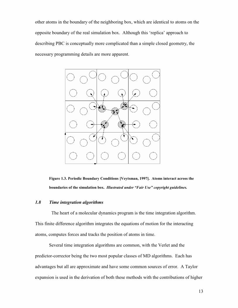
An alternative explanation of periodic boundary conditions is shown below in
Figure 1.3. A continuously updated copy of the simulation box is joined to each face of
the actual simulation box. An atom within the cut-off radius of a boundary is affected by I The similarity of the system with a closed, non-Euclidean geometry is limited since the angles of a triangle in the simulation box still add to 180˚.
13
other atoms in the boundary of the neighboring box, which are identical to atoms on the
opposite boundary of the real simulation box. Although this ‘replica’ approach to
describing PBC is conceptually more complicated than a simple closed geometry, the
necessary programming details are more apparent.
Figure 1.3. Periodic Boundary Conditions [Veytsman, 1997]. Atoms interact across the
boundaries of the simulation box. Illustrated under “Fair Use” copyright guidelines.
1.8 Time integration algorithms
The heart of a molecular dynamics program is the time integration algorithm.
This finite difference algorithm integrates the equations of motion for the interacting
atoms, computes forces and tracks the position of atoms in time.
Several time integration algorithms are common, with the Verlet and the
predictor-corrector being the two most popular classes of MD algorithms. Each has
advantages but all are approximate and have some common sources of error. A Taylor
expansion is used in the derivation of both these methods with the contributions of higher

14
order terms being neglected. Also, the precision implemented in the particular code will
ultimately cause round off errors. Both of these errors can be minimized by decreasing
the timestep and increasing the numerical precision set aside by the program [Haile,
1997].
Predictor-corrector methods advance the simulation in time by predicting an
acceleration with a Taylor expansion then later correcting the acceleration when the force
is formally evaluated from the gradient of the potential. These methods require eight
arrays of size 3N, which is five more than required by the popular Verlet schemes. A
specific interpretation is the Gear predictor-corrector, which is fifth order accurate and
can use a longer timestep than Verlet methods, thus making it both more accurate and
more stable [Haile, 1997].
The Verlet algorithm is a good compromise between accuracy and performance.
The MD algorithm in this thesis uses a Verlet variant known as the velocity Verlet
algorithm which explicitly includes the velocity in the algorithm and is therefore self
starting when provided positions and velocities. Although it is mathematically identical
to the standard Verlet scheme, the kinetic energy in the Verlet velocity algorithm may be
computed immediately rather than requiring an extra step to compute atomic velocities
[Haile, 1997].
Simulations involving external inputs such as external forces or artificially fixed
velocities add energy to the system and cause an increase in temperature. In this type of
simulation, it is often desirable to hold the system or a body within a system at a given
temperature. One convenient way of maintaining a fluid at a constant temperature is
modifying the equations of motion in the time integration algorithm. Velocities in the
region to be thermostated are rescaled upwards or downwards such that the desired
temperature is maintained. Actual velocities Vact are replaced with Vset:

15
(1.9)
where Tset is the desired temperature and Tact is the current temperature [Haile, 1997]. At
this point, Newton’s laws are no longer being used; an artificial velocity correction
proportional to T(t)-1/2 causes the actual velocity to converge to the velocity needed for
the set temperature. Although the thermodynamic properties of this system are identical
to that of a closed system, caution should be exercised if the trajectories of individual
atoms are followed. This method of temperature control will be adopted for this thesis,
but it is only one of several well known “thermostats”.

16
Chapter 2: Literature Review
2.1 Historical Background
A brief discussion of MD history and relevant past works is presented here to
properly position this research within the context of MD literature.
The principles of MD were well understood long ago, but without a computer
little could be accomplished. Not until the 1950s could MD even yield results for simple,
idealistic systems with a small number of particles. As the computer evolved, important
contributions were made in many fields ranging from crystalline defects in solids to
nanofluidics.
Researchers using MD find themselves in a situation opposite that of their
colleagues involved in experimental work; investigation at an ultra small scale turns out
to be easier than at the macro scale. It should be no surprise that atomic fluids were a
natural first application since an arbitrary number of atoms can form the volume of fluid
to be analyzed. Fluids, particularly liquids and rarified gases, still remain an open subject
in MD.
The first research reporting a molecular dynamics simulation was published by
Alder and Wainwright [Alder, 1957]. The work investigated the phase diagram of a hard
sphere system, particularly the solid and liquid regions. In a hard sphere system, particles
interact via instantaneous collisions and travel freely between collisions. Important
insights concerning the behavior of simple liquid simulations emerged from their studies.
Fluid properties were becoming a specialty of MD immediately after its conception, but
the sluggish vacuum computers of the 1950s were only suited for very small systems with
simple potentials. The above calculations were performed on a 25 ft x 50 ft UNIVAC
vacuum tube computer operating at 2.25 MHz.

17
The next major advance was in 1964, when Aneesur Rahman carried out the first
simulation using a realistic potential for liquid argon [Rahman, 1964]. Rahman is well
known as a founder of modern molecular dynamics and made important breakthroughs
concerning the properties of liquid argon and the Lennard-Jones potential. Although
Rahman’s work began as a method of modeling neutron scattering, it contained many of
the important features used in nanofluidic MD simulation today. The truncated LJ
potential, periodic boundary conditions and modern parameters for liquid argon were all
included. Rahman realized that liquid argon would be an ideal substance for simulation
because of its unique ability to be modeled by the LJ potential.
The algorithms used in MD were also improving at a fast rate. In 1967, Loup
Verlet introduced the bookkeeping scheme known as Verlet neighbor list. This
bookkeeping device kept a list of neighbor atoms within each atom’s cutoff radius plus an
additional length know as skin thickness. When an atom traveled outside the skin
thickness, the list was rebuilt so that an updated list of nearby atoms was always
available. The program no longer needed to check the coordinate of every atom to
determine which atoms were within the radius of the cutoff potential. Using the neighbor
list technique, only the distance to nearby atoms must be calculated at every timestep.
Neighbor lists are still considered a staple of MD code today. The celebrated Verlet form
of the time integration algorithm was also introduced [Verlet, 1967]. Verlet was able to
apply his new technique to match an actual phase diagram of liquid argon with one
calculated from directly from MD simulation. His system contained only 864 atoms.
Like Verlet, the majority of early researchers in this field derived transport properties
from equilibrium molecular dynamics, with viscosity being the most common subject.
NEMD simulation was later used to determine many of these same transport properties.

18
The obvious extension of NEMD was the modeling of classic Navier-Stokes
solutions such as Poiseuille and Couette flow, but a realistic investigation would only be
possible using the computer power of the 1980s. Publications related to boundary
conditions on a solid surface, Poiseuille flow, Stokes drag and other pieces of literature
relevant to this work are discussed below.
2.2 Poiseuille Flow
The modeling of Poiseuille flow accelerated in the late 1980s and 1990s. Koplik
et al. began an important line of research in the 1988, with their study of Poiseuille flow
and the no slip boundary condition [Koplik, 1988]. Basic properties of Poiseuille flow
were first established from a microscopic level and compared with those resulting from a
continuum assumption.
For a low Reynolds number flow though a channel, the well known parabolic
velocity profile was observed. This allowed the fluid’s viscosity to be determined by
matching a curve fit of the velocity profile to a Poiseuille flow solution. The no slip
condition was observed to arise naturally from the wall-fluid interaction.
In another work [Koplik, 1989], a continuum solution containing a divergence in
the shear stress at a moving contact line is resolved by MD simulation. A moving contact
line forms when two immiscible fluids meet on a translating solid surface. Applying the
no slip condition at the solid surface leads to an infinite stress at the contact line. The
situation may be resolved analytically by relaxing the no slip condition near the contact
line. Koplik et al. showed the physical reasoning behind this assumption through a
molecular dynamics simulation of Poiseuille flow involving the two fluids. The no slip
condition is shown to fail near the contact line but holds elsewhere along the surface.
Using MD to resolve divergences in continuum fluid mechanics would become a
common theme in the later work of this and other authors.

19
In the same publication [Koplik, 1989], Koplik also detailed the fluid’s behavior
closely, specifically near the wall. Fluid atoms were observed to form discrete, well-
defined layers near a wall of FCC (faced centered cubic) structure. There layers were
represented as sharp density oscillations that decreased in positions toward the center of
the channel. Further, fluid atoms near the FCC structured wall were most likely to be
found in a similar FCC arrangement. This study was not the first to observe organized
fluid structure near a surface, but certainly helped the formation of atomic layers near a
surface to become a well known observation in the nanofluidics community.
Koplik et al. also document velocity slip at low fluid densities. In a sequence of
densities from 0.8 to 0.08 N/σ3 (at a fixed temperature), a smooth transition to slip is
observed in Poiseuille flow. Continuum descriptions of velocity slip in rarified gas
support this observation.
The MD study of polyatomic fluids began with Rahman et al. in the simulation of
liquid water [Rahman, 1974]. More complex fluids have been modeled since and these
have been found to produce properties near to that of a continuum fluid in large enough
systems. Exceptions to the behavior predicted by a continuum description do occur when
a channel is narrow enough to cause a failure of the Navier-Stokes equations. This
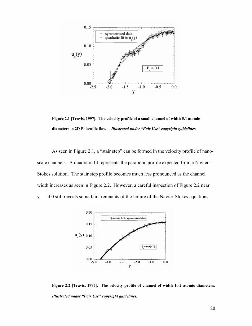
problem is addressed by Travis et al. [1997]. Channels having a width somewhat less
than 10 atomic diameters are seen to diverge from the parabolic velocity profile predicted
by Navier-Stokes calculations.
20
Figure 2.1 [Travis, 1997]. The velocity profile of a small channel of width 5.1 atomic
diameters in 2D Poiseuille flow. Illustrated under “Fair Use” copyright guidelines.
As seen in Figure 2.1, a “stair step” can be formed in the velocity profile of nano-
scale channels. A quadratic fit represents the parabolic profile expected from a Navier-
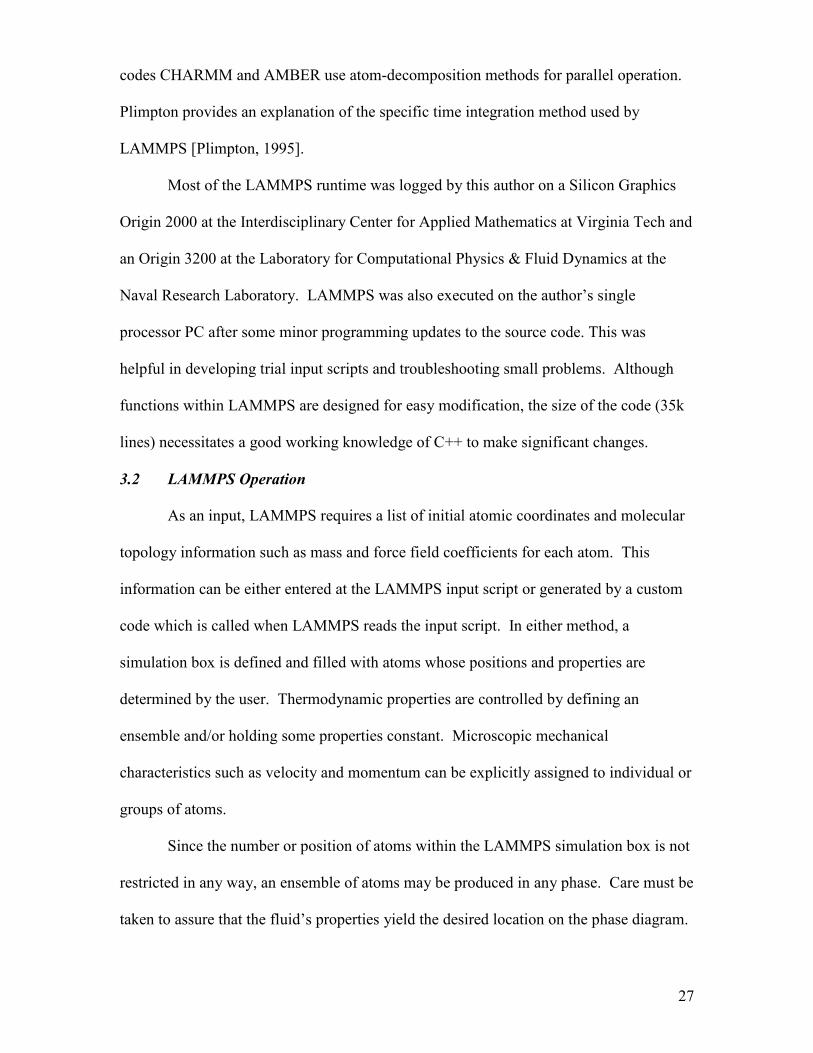
Stokes solution. The stair step profile becomes much less pronounced as the channel
width increases as seen in Figure 2.2. However, a careful inspection of Figure 2.2 near
y = -4.0 still reveals some faint remnants of the failure of the Navier-Stokes equations.
Figure 2.2 [Travis, 1997]. The velocity profile of channel of width 10.2 atomic diameters.
Illustrated under “Fair Use” copyright guidelines.

21
2.3 Drag Force and Stokes Law
The 1980s held several important accomplishments related to external flow,
including the exploration of eddies by D.C. Rapaport et al. [1986]. This work examined
the formation of eddies using 100,000 atoms with a simple, repulsive potential. It was
the first MD study of a large number of particles flowing around an obstacle.
Rapaport et al. simulated a two-dimensional flow past a circular obstacle with the
use of periodic boundary conditions. Fluid collisions with the obstacle were modeled as
both having a specular reflection, implying a slip boundary, and as having random
reflection, resulting in a no-slip condition. The choice of boundary condition was found
not to affect the results. At sufficiently large Reynolds numbers, the flow field
demonstrated characteristics of continuum fluids such as eddies, eddy separation and an
oscillating wake. The authors were able to directly compare their results to extensive
photographic documentation and continuum numerical solutions of eddy formation. The
Strouhal number, a nondimensional number associated with wake oscillation, of the
simulation was found to compare well with continuum data. D.C. Rapaport developed
one of the first parallel MD codes, which he used on four processors for this simulation.
Figure 2.3. Examples of wake oscillations from the back of a disk [Rapaport, 1986].
Illustrated under “Fair Use” copyright guidelines.

22
Next, an important work by Koplik et al. detailed the drag force associated with
an atomic sphere while undergoing either translation or rotation in an atomic fluid
[Koplik, 1996]. The modeling of the sphere’s translation served as both an inspiration
and starting point for this thesis. In Chapter 5, the drag force found in this reference is
used to confirm the initial modeling performed in this thesis.
The authors found several similarities with continuum results. In particular,
Stokes’ drag [Stokes, 1851] was found to match the MD solution closely. Stokes law
states that the drag force on a sphere moving at low Reynolds number through an infinite,
viscous fluid can be approximated as
(2.1)
where µ is the dynamic viscosity, b is the sphere radius and U is velocity of the sphere.
All of these parameters are known, so the continuum result is easily obtained and
compared with the drag force found from MD simulation. Rather than comparing drag
directly, the authors compute the sphere radius b and compare with the nominal sphere
radius. Agreement of the computed and nominal radii is found to be good at different
velocities and sphere sizes. The authors are also able to use MD to resolve two cases of
an unphysical divergence in solutions of the Navier-Stokes equations for a sphere near a
wall. Both divergences were rooted in the use of the no-slip condition.
As with previous studies, fluid density was observed to be heterogeneous near the
walls. The spontaneous layering of fluid is best documented by Barrat et al. [1994]. Six
visible, organized layers were observed as shown in Figure 2.4 below.

23
Figure 2.4. Density gradients across a channel bound by molecular walls [Barrat, 1994].
Illustrated under “Fair Use” copyright guidelines.
2.4 Wall Models
Koplik et al. employed a sphere that was held in shape by the large mass of the
individual atoms. Many walls in MD fluid simulations are modeled in a similar way
[Sun, 1992; Koplik, 1988, 1989, 1996] rather than employing more elaborate schemes
that require computationally expensive nonlinear springs [Travis, 1997] or other modified
bonds.
Sun and Ebner developed several wall models in the early 1990s and studied the
fluid-wall interface [Sun, 1992]. One interesting model combines a continuous 10-6 LJ
potential, the “heavy” type wall atoms mentioned above and a bonding potential between
the wall atoms. A uniform (non-atomic) wall having a continuous 10-6 LJ potential was
covered with six layers of atoms which were both heavier and had a more attractive
potential than the fluid atoms. This composite approach addressed some of the problems
with earlier wall models.

24
Ideally, walls should be made of a large number of layers connected by realistic
bonds; however, the amount of computational power available for simulating the fluid
would be reduced. Bonding between atoms in a solid, such as a wall, also allows heat to
be transferred in a realistic fashion at the expense of computation time. More wall layers
are required to maintain the stability of a structure connected by bonds than a structure
with atoms artificially held in place by some computational trick, such as giving the
atoms a large mass.
Molecular structure within the wall is important since a few layers of fluid
molecules tend to arrange themselves over the lattice sites of the wall; however, solid
continuous walls are not without benefit. A single potential can be defined for an entire
continuous wall, effectively making one large particle that replaces thousands of
individual wall atoms. The wall of Sun and Ebner [Sun, 1992] creatively combine the
advantages of both by using a molecular wall with a solid backing.
Later in 1990s, Koplik et al. led a more in depth investigation of the properties of
molecular walls [Koplik, 1998]. They found that if the precise structure of the molecular
wall is not important to the fluid behavior or, if behavior near the wall is not of interest, a
“thermal” wall could then be substituted for a more complex atomic wall. It was found
that walls can be stochastically treated as smooth surfaces that reflect fluid in a random
direction with a magnitude related to the wall temperature. This significant work also
clarified the mathematics of thermal walls and illustrated pitfalls in their application.
Thermal walls are much easier to implement than a full atomic description;
however the model conceals some of the properties of a real atomic wall and is not
widely used in NEMD.

25
2.5 Comprehensive References
Several useful texts were published in the 1990s that helped make MD accessible
to those outside of the field. Haile developed a text [Haile, 1997] which included general
techniques for solid and fluid systems that use hard sphere or LJ potentials. The book
contained basic considerations for MD simulation and developed examples using
FORTRAN code. This text still serves as an alterative for researchers not familiar with
the C language used in an earlier text by Rapaport [1995].
Although both books are similar, Rapaport’s book is the more practical for those
interested in creating a custom code. Rapaport developed the basic framework of an MD
program in a generic style of C code. In many ways, his text was also intended to be a
“cookbook” of sorts for MD calculations, as was further emphasized in the 2nd edition
published in 2004 [Rapaport, 2004].

26
Chapter 3: LAMMPS and Visualization Software
3.1 LAMMPS – Large Atomic Molecular Massively Parallel Simulator
LAMMPS is an open source, classical molecular dynamics code developed by
Sandia National Laboratories. It is a C++ code capable of modeling atomic, polyatomic,
biological, metallic or granular molecules using a variety of force fields and boundary
conditions. Biomolecular systems requiring detailed modeling are a common use of
LAMMPS simulation, thus the full potential of LAMMPS is not required for this work.
Only a single potential, a time integration scheme, a simple thermostat and some basic
preprocessing functions are needed.
Although LAMMPS runs efficiently on single processor workstations, it is
designed for parallel applications. The maximum number of atoms that can be modeled in
a simulation is dependent on computational power. In most atomic systems, the time
required for computing scales linearly with the number of atoms in the system. The same
linear scaling does not hold for the number of processors and limitations occur when any
code runs in parallel on a multiprocessor machine. The overhead associated with
communicating between processors becomes important and, given enough processors,
will eventually dominate the computational time. A maximum of only 16 processors was
used at any time in this work, meaning that most of the runtime is spent on molecular
dynamics rather than processor communication.
While running in parallel, spatial decomposition techniques are used to partition
the simulation box into three dimensional blocks which are divided among the
processors. Processors communicate and store ‘ghost’ atoms, i.e., information about
other atoms bordering the processor’s assigned region of space. Other MD codes such as
NAMD and NWCHEM also use spatial-decomposition approaches, however, the popular
27
codes CHARMM and AMBER use atom-decomposition methods for parallel operation.
Plimpton provides an explanation of the specific time integration method used by
LAMMPS [Plimpton, 1995].
Most of the LAMMPS runtime was logged by this author on a Silicon Graphics
Origin 2000 at the Interdisciplinary Center for Applied Mathematics at Virginia Tech and
an Origin 3200 at the Laboratory for Computational Physics & Fluid Dynamics at the
Naval Research Laboratory. LAMMPS was also executed on the author’s single
processor PC after some minor programming updates to the source code. This was
helpful in developing trial input scripts and troubleshooting small problems. Although
functions within LAMMPS are designed for easy modification, the size of the code (35k
lines) necessitates a good working knowledge of C++ to make significant changes.
3.2 LAMMPS Operation
As an input, LAMMPS requires a list of initial atomic coordinates and molecular
topology information such as mass and force field coefficients for each atom. This
information can be either entered at the LAMMPS input script or generated by a custom
code which is called when LAMMPS reads the input script. In either method, a
simulation box is defined and filled with atoms whose positions and properties are
determined by the user. Thermodynamic properties are controlled by defining an
ensemble and/or holding some properties constant. Microscopic mechanical
characteristics such as velocity and momentum can be explicitly assigned to individual or
groups of atoms.
Since the number or position of atoms within the LAMMPS simulation box is not
restricted in any way, an ensemble of atoms may be produced in any phase. Care must be
taken to assure that the fluid’s properties yield the desired location on the phase diagram.

28
Once the system constraints are set, LAMMPS updates the system by the Verlet
velocity integration scheme (see Section 1.8) over a predetermined number of timesteps.
Integration is prematurely stopped if values stored in the program, such as a
thermodynamic property, become unphysically large.
3.3 LAMMPS Pre- and Postprocessing
Several features are available within LAMMPS that automatically generate
lattices and simple geometric shapes. A built-in preprocessor can produce sets of atom
coordinates that correspond to different three-dimensional shapes. The LAMMPS
preprocessor takes user input for the specific shape and assigns the required atomic
coordinates to a text file. Both the wall and sphere of this thesis were generated with this
preprocessor. More complex geometries can be created by bypassing the default
preprocessor and inputting atomic coordinates via a text file; however, any geometric
figure must always built from a collection of individual atoms which are positioned by
the user.
Caution must be exercised as the atoms are being positioned. Any two atoms
placed unnaturally close together can produce a near infinite repulsive force, which leads
to a large temperature on the following timestep. The unexpectedly large force originates
from the steep slope of the LJ potential near R=0 and is completely avoidable by a proper
choice of atomic spacing. Despite its simplicity, this is a common problem. Each atomic
position is defined by an algorithm that writes Cartesian coordinates to a text file, thereby
assuming atoms to exist only as points. The algorithm is chosen to space these points
properly but exceptions can occur near boundaries of two geometric regions or on the
border of the simulation box when periodic boundary conditions are applied.
Most commonly, an atom located on one plane of the simulation box is
accidentally imposed over another atom on the opposite side by periodic boundary

29
conditions. The proximity of the two atoms produces a large temperature that crashes the
program. Locating the offending atom(s) is not always trivial and the details of the input
script can become important in resolving these conflicts.
No postprocessing operations are available with LAMMPS. Postprocessing
duties are handled by a multi-functional code created by the author. This code allows the
user to find the instantaneous drag force, average net drag force and atomic velocity
distribution over a range of timesteps. These quantities and related data are printed to a
text file so that further analysis can be performed with a spreadsheet program.
3.4 Visual Molecular Dynamics
Despite being one of the simplest forms of data analysis, having a visual output is
vitally important in molecular dynamics. During the research documented in this thesis,
the system exhibited unusual flow patterns, freezing, loss of atoms and other unexpected
phenomena. Each time the unusual event could be immediately observed from the
visualization and traced back to a minor mistake in the input script. Subtle mistakes,
especially syntax problems, are easily overlooked in the input script but rarely go
unnoticed in the visualization.
Although several good visualization codes exist, Visual Molecular Dynamics
(VMD) is used throughout this work. VMD is specifically designed for visualizing
biological and molecular systems and, like LAMMPS, it is more than adequately
equipped to handle a flowing atomic fluid. The Theoretical Biophysics Group at the
University of Illinois at Champaign developed this open source code for public use
[Humphrey, 1996].
VMD provides a way of animating an otherwise abstract collection of data.
LAMMPS provides the coordinates for all the atoms of the simulation to VMD over a
series of timesteps in the form of a properly-formatted text file. Because the atoms are

30
represented by only a set of coordinates, a common approach to visualizing an atom is to
assign a radius from the coordinate and fill the volume inside this radius with a solid
color. Despite its ad hoc nature, the sphere has a counterpart in the repulsive core of the
LJ potential, or in a more physical sense, the electron cloud of a real atom.
VMD has a large variety of color schemes and visualization styles. The user may
choose to work with the excellent VMD graphical interface or use the command prompt.
A screenshot is shown below in Figure 3.1.
Figure 3.1. VMD interface. Illustrated under “Fair Use” copyright guidelines.

31
Chapter 4: Development of Biosensor Inspired Problems
As discussed briefly in Chapter 1, drag on a nano-size sphere near a wall has
interesting applications in biosensor design. In the future, BARC and FDB type
biosensors could use nano-size beads to “label” the detection of a specific biological
molecule in the same way that micron-size beads do today.
In the case of the BARC biosensor, a fluid containing single strand DNA is
pumped through channels which are lined with complementary DNA strands. If a
targeted biological agent is present, hybridized DNA pairs result. Beads are then pumped
through the channel and bond to the hybridized pairs. The FDB operates similarly,
except that sample single-strand DNA is attached directly to the bead rather than being
pumped through the channel in a preliminary step. Any beads which are not bound are
removed with magnetic (BARC) or fluidic (FDB) forces. The intensity of the remaining
bonded beads label the presence of a targeted biological agent [Gijs, 2004].
A known limitation to any “bead labeling” approach is the background noise
created from uncaptured beads, i.e., those unbound beads which remain in the biosensor
while the bound beads are being counted. These unbound beads will be more numerous
if the force required for removing the beads is not well understood, thus leading to the
problems investigated in this thesis. A biosensor can be physically smaller if nano-size
rather than micro-size beads are used as labels; however, the force needed to remove an
unbound ‘nanobead’ is not well understood. This thesis takes a first step toward enabling
the eventual use of nanobeads by investigating the drag forces which act on both a
nanobead and a planar surface.
Insight into the magnetic or fluidic forces needed to remove unbounded beads can
be gained by finding the drag on a single nanobead at different positions within the
biodetector and at different Reynolds numbers. MEMS and NEMS devices have a large
32
surface to volume ratio, making the near-wall behavior of the bead and the skin friction
on the inside surface of the biosensor important. In particular, knowledge of the
following quantities is useful:
Problem 1: Drag acting on an isolated sphere. The drag coefficients of a
nanosphere in an infinite fluid are found as a function of nanosphere
velocity. A range of Reynolds numbers between 1.98 and 8.0 are
considered.
Problem 2: Drag acting along a wall. The skin friction coefficients of a wall are
determined for a variable wall density at a fixed velocity of 2.0σ/τ.
Problem 3: Drag acting on a sphere near a wall. The drag coefficients of a
nanosphere near a wall are determined at a fixed velocity of 2.0σ/τ.
Seven separate distances are considered.
Setting up, solving, and critically examining the results of these three basic problems is
the goal of this thesis. The problems are divided into three sets of simulations, which will
be termed “research runs”. Before any research runs are carried out, LAMMPS will be
applied to a validation problem of which the setup and simulation is the topic of
Chapter 5.

33
Chapter 5: Validation of the LAMMPS Code
5.1 The Need for a Validation Problem
The validation case here was based on the work of Koplik et al. [1996] and
described in Section 2.3. They used MD simulation to determine the drag on a
nanosphere in an infinite fluid and compared these results with Stokes law. In this
chapter, one of these drag calculations is repeated and compared with the results of
Koplik et al. The details of the setup and simulation of this problem are described below.
5.2 Modeling Considerations
Koplik et al. [1996] describe a solid sphere, constructed from individual atoms,
moving through an atomic liquid. Moving an object through a stationary fluid is unusual
when compared to the “wind tunnel” approach typically used in experimental and
computational aerodynamics in which fluid flows over an object. The field of MD
developed independently of aerodynamics in the 1960s as a study of stationary fluids and
gradually acquired a culture of fluid-centric rather than body-centric simulation. The two
methods are equivalent; however, the traditional reference frame of a stationary fluid is
used in this workII.
Many of the parameters of Koplik et al. [1996] are duplicated in this thesis, with
the notable exception of the simulation box dimensions and the need for a permeable
vertical wall (both described later). As in the work of Koplik et al., nondimensional LJ
units are used throughout the simulation. Length, temperature and mass are
nondimensionalized with σ = 3.4Å, ε/kb = 120K, and m = 40 amu, respectively. The
natural time unit is then τ = σ·√(m/ε) = 2.16·10-12 sec.
II The simulation of Section 5.5 was modeled using both a stationary fluid and a moving fluid propelled by a piston. The two approaches yielded a drag result within 3% of one another.

34
The fluid of the problem is created first. Roughly 25,000 fluid atoms are assigned
at points on an FCC lattice that completely fills the simulation box. Each fluid atom has
a mass of 1m and all atoms interact via the LJ 12-6 potential function. The
nondimensional density of 0.8m/σ3 and FCC structure of the fluid are identical to Koplik
et al. [1996]. A void for placement of the sphere is created by deleting fluid atoms inside
of a radius 2.1σ centered at X = 6, Y = 15, Z = 6 in the simulation box. See Figure 5.1 for
coordinate system.
The sphere is duplicated from Koplik et al. [1996] by forming a separate FCC
lattice with a density of 1.8 m/σ3 and extracting the atoms inside a radius of 2σ. These 56
atoms are then centered in the void described above. Atoms in the sphere are not allowed
to interact with each other but do interact with the fluid atoms with a LJ 12-6 potential.
Interactions among the sphere atoms can cause a slow increase in radius which may
influence the drag force. These atoms are given a very high mass of 1.8·106m for reasons
explained in Section 5.4.
The two principal stages of the simulation will now be carried out. During the
first stage, a crystalline solid will be melted to form a fluid. In MD literature, this process
is known as “equilibration”. Once the solid is completely melted, the sphere will travel
through the fluid in a NEMD simulation.
5.3 Equilibration of the System
Atoms are initially melted from an FCC lattice by imposing a temperature on the
solid that is above its melting point. A temperature of 1.2ε/kB (144K) is applied in this
case, giving atoms a sufficient kinetic energy to break the attractive bonds of the LJ
potential and move around the simulation box.
After some time, all traces of the well ordered solid shown in Figure 5.1 are lost
and replaced with random thermal motion – this occurs when the system has concluded

35
the equilibration process and reached a stable equilibrium state. The transformation to a
liquid must be complete, thus requiring that the final temperature and density of the fluid
lie within the liquid region of the phase diagram.
Figure 5.1. The fluidic system as a solid. Atoms are shown as enlarged points to
illustrate the FCC lattice structure of the fluid. Stripes in the fluid are a result of the FCC
lattice structure and do not indicate any nonuniformity in the atomic spacing.
Figure 5.1 shows the actual fluid system before the equilibration process was
started. The need for the permeable wall shown on the left face of the simulation box is
discussed in Section 5.4.
The achievement of an equilibrium state can be recognized by several markers.
From a macroscopic (thermodynamic) point of view, the system’s entropy must be a
maximum. Unfortunately, entropy is not a physical quantity that lends itself to
measurement and its direct calculation from the microcanonical ensemble is limited to
trivial systems. However, it is possible to detect the attainment of an equilibrium state,
with a reasonable degree of certainty, by the observation of other parameters [Haile,
1997].

36
One such observation is the fluctuation of instantaneous thermodynamic
properties about a running average that is independent of the simulation time. Another
requirement is that the time average of each atom’s Cartesian component of velocity
follow a Maxwell velocity distribution [Haile, 1997]. The Maxwell velocity distribution
is a Gaussian distribution with standard deviation s = (kT/m)1/2 and mean velocity <v> =
0. It is defined as
(5.1)
where T is temperature of the fluid. One component of the velocity distribution of fluid
atoms taken at the end of an equilibrium simulation is illustrated in Figure 5.2 below.
0
50
100
150
200
250
300
350
400
450
0 10 20 30 40 50 60 70 80 90 100
Velocity (% of maximum)
Num
ber o
f A
tom
s
Figure 5.2. Velocity distribution of fluid atoms at 50τ (shown for one degree of freedom).
The speeds predicted by the Maxwell distribution are shown with a solid line.

37
The Maxwell velocity distribution is shown only for positive velocities acting in
the X direction. Negative velocities and velocities acting in other Cartesian directions
have an identical Maxwell distribution.
The distribution shown in Figure 5.2 occurs after a time of 50τ. At this point, the
temperature and pressure of the system were observed to show fluctuations with a
magnitude less than 1% of the average. From combined inspection of thermodynamic
properties and the velocity distribution, it was concluded that the system was
equilibrated.
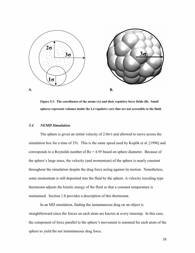
Comment: The interpretation of the sphere’s radius must now be adjusted since the
radius inaccessible to fluid is different than the radius created in Section 5.2. As
discussed in Chapter 1, atoms behaving according to the LJ potential experience a rapidly
increasing repulsive force when moving within roughly 1σ of another atom. Atoms on
the surface of the sphere apply this repulsive force to nearby fluid atoms and therefore
cause the sphere to behave as if the radius has been increased by 1σ. Figure 5.3 below
illustrates how the “nominal” radius of the sphere is measured.
38
Figure 5.3. The coordinates of the atoms (A) and their repulsive force fields (B). Small
spheres represent volumes inside the LJ repulsive core that are not accessible to the fluid.
5.4 NEMD Simulation
The sphere is given an initial velocity of 2.0σ/τ and allowed to move across the
simulation box for a time of 35τ. This is the same speed used by Koplik et al. [1996] and
corresponds to a Reynolds number of Re = 4.95 based on sphere diameter. Because of
the sphere’s large mass, the velocity (and momentum) of the sphere is nearly constant
throughout the simulation despite the drag force acting against its motion. Nonetheless,
some momentum is still deposited into the fluid by the sphere. A velocity rescaling type
thermostat adjusts the kinetic energy of the fluid so that a constant temperature is
maintained. Section 1.8 provides a description of this thermostat.
In an MD simulation, finding the instantaneous drag on an object is
straightforward since the forces on each atom are known at every timestep. In this case,
the component of force parallel to the sphere’s movement is summed for each atom of the
sphere to yield the net instantaneous drag force.
A.
1σ
3σ 3σ
2σ
B.
39
Using completely periodic boundaries on the simulation box caused the sphere to
experience a drag force with a magnitude that was too small. The momentum in the
direction of the sphere’s movement exited the simulation box in front of the sphere and
reentered behind it. This circulation of fluid caused the magnitude of the drag force to
continuously decrease as the sphere moved further along the simulation box. Placing a
solid wall at the end of simulation box could have completely prevented the momentum
transfer; however, the simulation results of this author found that the drag force’s
magnitude increased with the presence of a solid wall. Analytical results [Brenner, 1961]
also show that a sphere moving perpendicular to a solid wall will experience an increased
drag as it approaches the wall. For this reason, a hybrid method was used to allow some,
but not all, of the fluid momentum to move through the wall.
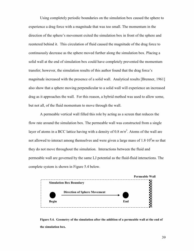
A permeable vertical wall filled this role by acting as a screen that reduces the
flow rate around the simulation box. The permeable wall was constructed from a single
layer of atoms in a BCC lattice having with a density of 0.8 m/σ3. Atoms of the wall are
not allowed to interact among themselves and were given a large mass of 1.8·106m so that
they do not move throughout the simulation. Interactions between the fluid and
permeable wall are governed by the same LJ potential as the fluid-fluid interactions. The
complete system is shown in Figure 5.4 below.
Figure 5.4. Geometry of the simulation after the addition of a permeable wall at the end of
the simulation box.
Permeable Wall
Direction of Sphere Movement
Simulation Box Boundary
Begin End

40
While using the setup shown in Figure 5.4, it was observed that the drag force on
the sphere remained at a time invariant (steady-state) value when the sphere was near the
center of the simulation box.
5.5 Validation Results
Although the sphere is moved through the fluid for a total time of 35τ, the first
15τ (a distance of 30σ) is needed to yield a steady-state drag value. Drag data is
considered only after the initial transient period has passed and before the sphere
approaches the permeable wall. As in Koplik et al. [1996], the drag force is sampled
every 0.25τ and the mean drag force is calculated over 12.5τ. The mean drag as a
function of time is shown in Figure 5.5 (solid line).
-450
-400
-350
-300
-250
-200
-150
-100
-50
0
5 7 9 11 13 15 17 19 21 23 25 27 29
Time (τ)
Drag Force
( mσ/τ^2)
Transient Period Data Collection Period
Figure 5.5. Transition to Steady-State Drag at Re = 4.95. Instantaneous drag measurements
are shown as diamonds.

41
The variation of the instantaneous drag force is not intuitive. Despite the sphere’s
composition of 56 individual atoms, with many of those being exposed to the fluid, the
drag force in Figure 5.5 (shown as diamonds) rarely resembles the running average of the
drag force (solid line). Our confidence can be improved by putting these results in a
statistical context. An analysis (not shown) of the “Data Collection Period” in Figure 5.5
reveals that the drag data follows a roughly Gaussian distribution which has a mean equal
to the running average. A uniform distribution would be expected if the drag data
occurred randomly.
To form a comparison with Koplik et al. [1996], the mean drag will be expressed
as a computed radius obtained with Stokes law. The drag acting on the sphere in the
steady-state condition leads to a computed radius of 2.816σ. This is 7% less than the
nominal radius of 3σ and 10% less than the computed radius of 3.1±0.3σ reported by
Koplik et al.
The computed radius found by Koplik et al. has an uncertainty large enough to
include the computed radius of this validation problem. It is therefore concluded that the
drag results calculated here are reasonable and that the problem-solving approach taken
in this chapter will yield valid drag results for the problems discussed in Chapter 4.
Comment: Although the results of this thesis and Koplik et al. are within the limits of
uncertainty, a possible explanation for the larger radius of Koplik et al. comes from the
setup of the problem. Rather than terminating the simulation box with a permeable wall,
a solid wall was used. Koplik et al. state that the simulation box is long enough to ignore
boundary effects. The simulations of this research did not lead to the same conclusion – a
solid wall was seen to increase the drag force significantly during the final 30% of the
simulation.

42
Chapter 6: Setup of the Research Runs
Before presenting the results of the research runs, it will be helpful to discuss a
few aspects of the modeling that will be needed to carry out these calculations. First,
those elements of the research runs which are in common with the validation case
discussed in the previous chapter are described. Then, since Problems 2 and 3 require the
addition of a wall to the simulation, how this is done will be described. Following this,
the sizing of the computational region will be described. Finally, because each research
run will later be compared with results of a Navier-Stokes solution, the chapter concludes
with a consideration of various issues which are related to the validity of that comparison.
6.1 Similarities with the Validation Case
The production runs and the validation case have much in common. In particular,
the design and placement of the sphere and permeable wall are taken directly from the
validation case. In addition, the fluid properties, the fluid equilibration process, and the
fluid thermostat are also identical to those used in Chapter 5.
As in Chapter 5, the collection of drag data begins with sphere’s center at a
distance of 6σ from the front edge of the simulation box and a constant drag value is
observed after a distance of 30σ has been traveled. The drag force in each research run is
then sampled every 0.25τ over 12.5τIII and averaged to produce a mean drag force.
6.2 The Modeling of the Wall
The wall was modeled by a collection of roughly 2000 atoms that interact with the
fluid using the 12-6 LJ potential but do not interact with each other. The wall was built
with an FCC lattice structure that has a different density in each of the five simulations of
III At Re = 8.0, the distance needed to reach a steady-state drag force is less than 30σ. The shorter approach to steady state allows an additional length of simulation box to be used for measuring the steady-state drag. By traveling this additional length, the sphere is able to meet the time requirement of 12.5τ in a steady state condition.

43
Problem 2 and a fixed density in Problem 3. No roughness beyond the discreteness of the
atoms is introduced and, like the atoms in the sphere, the wall atoms were given large,
non-physical masses of 1.8·106m.
The wall is located at the bottom of the simulation box and has a thickness of two
atomic layers to prevent the fluid near the upper boundary of the simulation box from
influencing fluid near the lower boundary via periodic boundary conditions. Using a
double-layer wall provides more fluid separation than the LJ potential cutoff of 2.5σ,
meaning that fluid atoms cannot interact with other fluid atoms through the wall. The
position of the wall is shown below without fluid present (A) and in a diagram of the
simulation box (B).
Figure 6.1. The atomic wall of density 1.8 N/σ3 with FCC packing structure (A) is located at
the bottom of the simulation box and duplicated by periodic boundary conditions (B).
It must be noted that the wall and sphere used in the research runs are not
intended to represent specific materials. At the temperature and pressure of the
simulation, a more complex potential function or quantum mechanical approach is
needed to form a real solid and atomic separations are, in turn, governed by such
considerations. Solids using these complex potentials are computationally more
A B

44
expensive than the LJ solids used in these simulations. Accuracy then has been traded for
simplicity.
In this connection, it is important to realize that the sphere used here (and the wall
as well) could not remain intact if the atoms were assigned a smaller, more physical mass
and allowed to interact with one another. The atomic spacing is smaller than preferred by
the LJ potential, and if left unchecked would cause the sphere to expand into the fluid.
As described in Chapter 5, the expansion of the sphere is easily prevented by turning off
the interactions among the sphere atoms, and this procedure is again used here.
Since the wall (and the sphere) are not actual materials, this introduces the atomic
density of the wall as another variable. Thus in the description of the results of Problem
2 in Chapter 7, the density of the wall will be treated as a variable.
Varying the density of the wall has consequences. The drag force on a body
whose atoms behave according to a two-body potential will depend heavily on the
number density used. Each fluid atom near the surface must interact with all the surface
atoms within its cutoff radius, thus resulting in a stronger fluid-surface interaction as
number density increases.
6.3 Sizing the Simulation Box
For the sake of consistency, it was decided to use the same size simulation box for
all of the three problems. The size of the simulation box must therefore meet the needs of
all problems. The considerations which resulted in the simulation box having
dimensions of 70σx40σx12σ will be described in the following paragraphs.
The length of the simulation box is the dimension parallel to movement of the
sphere. It is sized by considering the distance required by the sphere to reach and
maintain a steady-state drag force. The validation problem of Chapter 5 requires steady-
state drag to be maintained for 12.5τ; the same standard is applied here. As described in

45
Section 5.5, the sphere is observed to develop a steady-state drag after a distance of 30σ
(15τ), meaning that a total runtime of 27.5τ and a total length of 55σ is required. A
length of 6σ is added to this minimum requirement since the sphere does not start at the
beginning of the simulation box and an additional 9σ is added so that larger Reynolds
numbers can be accommodated. The total length of 70σ was found to be large enough to
allow a reliable measurement of drag force in the above sense for all three cases.
The height of simulation box is the dimension perpendicular to plane of the
bottom wall. A simulation box with a height greater than that used in the work of Koplik
et al. [1996] was needed to negate the effect of the wall’s replica appearing above the
simulation box as shown in Figure 6.1B above. The combination of the two walls results
in what is effectively Poiseuille flow with a slip condition at the walls. The “upper” wall,
a product of the periodic boundary conditions, must have a large enough separation from
the lower wall so as not to significantly affect flow patterns in the bottom half of the
simulation box. The required height is found by increasing the displacement of the two
walls until the drag on a sphere at the center of the simulation box matches the results
obtained in Chapter 5, which correspond to an infinite wall separation. A total required
height of 30σ was found to be necessary to assure this and an extra 10σ was added as a
safety factor.
The width of the simulation box (12σ) was small in comparison with its length
and width. It needs only to be wide enough so that the effect of the periodic boundary
conditions does not substantially interfere with the drag force. It was assumed that the
12σ width used by Koplik [1996] was sufficient for this purpose.

46
6.4 Comparing with Continuum Results
The author is not aware of any MD simulations with which Problems 2 and 3 can be
compared. In their absence, one alternative is to compare with Navier-Stokes solutions of similar
problems. This comparison needs to be viewed with care.
One issue is the adequacy of a continuum solution for these problems.
Fortunately, the Knudsen number (the ratio of the mean free path to the characteristic
dimension of the problem) is high enough (0.01 to 0.1) so that this is not a concern. In
this Knudsen number range, both the Navier Stokes (continuum) solutions and the MD
(particulate) solutions to these problems are valid.
The issue of the proper choice of boundary conditions to be employed in the
Navier Stokes calculations is more problematic. This is because in this range of Knudsen
number neither no-slip or pure slip boundary conditions are appropriate [Panton, 2005],
but rather something in-between, and the author is unaware of any rigorous way of
determining just what the appropriate boundary condition would beIV. In the following
chapter, comparison with Navier Stokes solutions employing both no-slip and pure slip
boundary conditions are made with the intent of providing reasonable limits with which
the MD simulations can be compared.
IV Using MD simulation does not resolve this problem, unless a potential which represents the actual solid-fluid interaction is used. In this work the same potential was used for the solid-fluid interaction as for the fluid-fluid interaction.
47
Chapter 7: Results of the Research Runs
Information concerning the results for each of the three Research Runs can be
found in this chapter. To build confidence in the results, they are compared with the MD
solutions of similar problems where possible and with Navier Stokes solutions in the
cases where an MD solution is not available.
7.1 Problem 1: Drag on an Isolated Sphere
This section describes the problem of calculating drag on a nanosphere in an
infinite fluid. This problem is identical to validation problem of Chapter 5, the only
difference being that the simulation has been carried out for six Reynolds numbers
between 1.98 and 8.0, rather than a single Reynolds number of 4.95. The results are
shown in Figure 7.1.
Good agreement with the results of Koplik et al. is seen at both of the Reynolds
numbers used in their calculations (1.98 and 4.95). Data at Reynolds numbers less than
Re = 1.98 could not be collected due to a large uncertainty in the mean drag force. This
is because at a low velocity, the magnitude of the drag force on the sphere is comparable
with thermal noise caused by interactions with fluid atoms. Extracting useful data
becomes impossible in this condition.

48
0.00
1.00
2.00
3.00
4.00
5.00
6.00
7.00
8.00
9.00
10.00
11.00
12.00
0.0 1.0 2.0 3.0 4.0 5.0 6.0 7.0 8.0 9.0 10.0
Reynolds Number
Drag C
oeff
icie
nt
Koplik, 1996
Koplik, 1996
Figure 7.1. Drag coefficient of a nanosphere at several Reynolds numbers.
To better understand the nature of the boundary conditions, it is useful to compare
these results with two Navier Stokes solutions; one employing no-slip and the other a
variable slip boundary condition. The no-slip result is given by the well-known Stokes
solution while the variable (between pure slip and no-slip) result is given by the work of
Happel et al [1967]. Both the Stokes and the Happel et al. results can be considered (for
their particular boundary conditions) minimum drag results since they correspond to
conditions of very low Reynolds numbers. Figure 7.2 illustrates Stokes law, the Happel
et al. results for a pure slip condition and the MD results.

49
Figure 7.2. Drag force as a function of Re from MD and Navier-Stokes equations.
As discussed in Section 6.5, the Knudsen number of this simulation indicates that
some slip is present, thus suggesting a lower drag value than that given by Stokes law.
This is in fact observed in Figure 7.2. Further, Figure 7.2 indicates that the values of drag
obtained in this problem are greater than the pure slip results, as they must be. Clearly
this supports the Knudsen-number-based argument of Chapter 6 in which a boundary
condition between that of pure slip and no-slip should be expected. Further supporting
this argument is the fact that a visualization of the sphere using the VMD tool described
in Chapter 3 shows that the fluid atoms slip along the sphere's surface. The fluid
behavior appears as a continuous slip – not the stick/slip mechanism sometimes observed
experimentally in microfluidics.

50
The drag coefficients from MD simulation are very close to the pure slip
condition (bottom curve) in Figure 7.2. This is interesting since the Knudsen number of
the flow suggests a boundary condition more near to a no-slip condition than a pure slip
condition. The qualitative nature of the Knudsen number argument may contribute to this
difference as well as need for an improved fluid-solid interaction in the MD simulation.
7.2 Problem 2: Friction on a Wall
This section describes the problem of calculating the friction along a wall as a
function of the wall’s number density.
Friction is evaluated along the length of the simulation box by moving the entire
wall through the fluid at a velocity of 2.0σ/τ but only observing forces on the atoms
within a 6σ x 6σ sample area. The instantaneous friction is found by summing the
horizontal force on each atom in the sample area, which is similar to the drag calculations
in Chapter 5 except that the friction is evaluated on only a portion of the wall. Only half
of the friction is used to calculate a skin friction coefficient since periodic boundary
conditions cause the fluid to exert force on both sides of the wall.
Figure 7.3. Position and motion of the wall.
6σ x 6σ
Area
Direction of Wall Motion 6σ
3σ
Fixed
Permeable
Wall

51
When the wall (initially at rest) is given a fixed velocity, the friction displays a
transient behavior similar to the sphere of validation problem and then settles into a
steady-state behavior which is independent of the computational time. Figure 7.4
illustrates the steady-state skin friction coefficient as the density of the wall is varied
from 1.0 to 5.0 N/σ3 in intervals of 1.0 N/σ3. Drag is expressed as the skin friction
coefficient, defined as
(7.1)
where ρ is the density, U is the fluid speed, A is the sample area and F is the friction
acting on the sample area.
0.00
0.05
0.10
0.15
0.20
0.25
0.30
0.0 1.0 2.0 3.0 4.0 5.0 6.0
Density N/σ^3
Skin
Fric
tion C
oeff
icie
nt
.
Blasius Solution
3.6
Figure 7.4. Relationship of drag coefficient and number density for a Lennard-Jones wall.
The linear dependence of the skin friction on density was expected since the
number density of the solid is directly proportional to the number of wall-fluid
interactions (forces) at the solid’s surface.

52
Although the Knudsen number of this problem indicates that a slip condition is
more appropriate, a comparison with a known analytical solution can give perspective to
the skin friction coefficients found here. The Blasius solution, which describes the
behavior that would be expected in a similar continuum problem if the no-slip condition
were applicable, can predict the drag coefficient as a function of the sample area’s
displacement from the front edge or “leading edge” of the simulation box. The skin
friction coefficient as determined from the Blasius solution is given by the following
relationship:
(7.2)
This expression is valid for laminar flows only [Panton, 2005]. A maximum Reynolds
number of Re = 44.5 is calculated for the flow in this problem – well within the limits of
laminar flow.
The characteristic length applicable to the Reynolds number in the Blasius
solution is the distance from the leading edge of the plate, thus a mean skin friction
coefficient can be obtained by evaluating the integral average of Equation 7.2 between
30σ and 54σ. The mean skin friction coefficient of the Blasius solution was found to be
Cf = 0.114.
It is interesting that the Blasius result may be matched to an effective wall density
as shown in Figure 7.4. Although a wall of this number density will produce the same
mean drag coefficient as predicted by the Blasius solution, it does not produce the
position dependent boundary layer also predicted by the Blasius solution. All of the skin
friction coefficients determined here were seen to be independent of position.
53
Comment: During equilibration, a VMD visualization showed fluid atoms forming
loosely ordered layers near the surface of the wall. Voids between these layers were
especially obvious surrounding the 1st and 2nd layer of fluid. It is likely that that a similar
phenomenon exists around the sphere of Section 7.1, however, a visualization of the
solid-liquid interaction is more difficult since the fluid completely surrounds the sphere.
7.3 Problem 3: Drag on a Sphere near a Wall
This section describes the problem of calculating the drag on a sphere near a wall
as a function of the sphere-wall separation. The geometry is a combination of Problem 1
and Problem 2; however, the wall is now created with a constant density which is equal
to that of the sphere of Problem 1. There is no relative motion between the sphere and
the wall – both move simultaneously through the fluid at a speed of 2.0σ/τ (Resphere =
4.95).
Drag on the sphere is measured at seven sphere-wall separations which ranged
from 26σ to zero. At a separation of zero, the lowest atom of the sphere is allowed to
contact an upper atom of the wall. Figure 7.5 shows the resulting drag coefficients and
their corresponding sphere-wall separation.

54
Figure 7.5. Drag coefficient of a sphere as a function of separation from a wall. Analytical
results are from Goldman [1967].
The drag at a sphere-wall separation of 15σ and greater is essentially the drag of a
sphere in an infinite fluid and corresponds to the results of Section 7.1 (at Re = 4.95). As
seen in Figure 7.5 above, the drag of the sphere decreases as it approaches the wall until
reaching a minimum when in contact with the wall. Numerical results in the continuum
regime from Sandberg [2002] (not shown) also indicate that a sphere affixed to a wall
experiences a significantly reduced drag force compared with the drag of a sphere in the
freestream.
Goldman et al. [1967] found an analytical solution for the drag on a stationary
sphere as a function of distance from a stationary wall. In Goldman’s case the velocity
profile is linear (uniform shear flow), which contrasts with the parabolic velocity profile
of this problemV. In order to compare with Goldman et al., an equivalent linear velocity
V The parabolic profile is a result of periodic boundary conditions producing a second wall above the simulation box. These walls both drive the flow, thus creating a velocity profile similar to Poiseuille flow.

55
profile is needed. The equivalent linear shear in this problem will be taken as the
average rate of change of velocity between the wall and the half-height of the simulation
boxVI. Using the equivalent linear profile in Goldman’s solution produces the drag
coefficients which are represented by the dashed line in Figure 7.5.
The results of Goldman et al. and MD are in surprisingly close agreement for
small sphere-wall separations, especially when the sphere is in contact with the wall. This
agreement is interesting since the fluid has a minimum Knudsen number which suggests
the use of a slip condition rather than the no-slip condition used by Goldman. It is
speculated that, in this problem, errors associated with forming an equivalent linear
velocity profile cause the two results to agree more closely than would otherwise be
expected. A more accurate comparison with results that employ a no-slip condition (such
as a numerical solution of the Navier-Stokes equations), would likely yield drag
coefficients that are greater than those of the MD solution.
Clearly, the Goldman results do not match well with the MD results as the sphere
moves away from the wall and into the center of the channel; however, a close match of
the two results cannot be expected since the linear and parabolic velocity profiles are
much different in this region.
VI The no-slip condition is assumed at the wall.

56
Chapter 8: Suggestions for Future Work
This work considers a range of Reynolds numbers (1.98 to 8.0) guided by the
work of Koplik et al. [1996]. In practice, the Reynolds number of flows on the micro- or
nano- scale is usually much less than 1.0 and often less than 0.1. If we find the velocity
from the median Reynolds number, we see that the sphere moves at a surprising 314
meters per second - obviously the Reynolds number of this flow would be much larger if
not for the very small size of the sphere. A new set of simulations are needed to the
determine drag coefficients of both an isolated nanobead and a nanobead near a wall at
much lower velocities.
As discussed in Section 7.1, determining the drag force on a sphere in a low
Reynolds number flow is difficult with the “translating sphere” approach taken by Koplik
et al. [1996]. A new approach must be found so that physically useful (low Re) results
can be produced. To avoid the problems of drag force measurement in low Reynolds
number flows, it is desirable to eliminate as many variables as possible that influence the
drag result, including the permeable wall and the limited running time of the simulation.
Two alternatives exist that would meet these needs.
A NEMD simulation of a fluid moving around a stationary sphere would allow
the instantaneous drag force to be monitored for any amount of time and would not
require a permeable wall to be present. In this setup, fluid travels through the front of
the simulation box, over the sphere, out the end of the simulation box and returns to the
beginning via periodic boundary conditions. The fluid is reset to the freestream
conditions before approaching the sphere. This simulation is the equivalent of the
experimental device typically used in continuum regime fluid dynamics, i.e., the wind
tunnel.

57
As a second approach, the Einstein-Stokes relation provides an opportunity to
establish the drag force on a sphere with no bulk movement of the sphere or fluid and
without a thermostat. This result, from Einstein’s famous study of Brownian motion in
1905, relates the diffusion coefficient to the drag coefficient of an object in a low
Reynolds number flow. A simulation using this approach has the great advantage that the
diffusion coefficient may be measured in an equilibrium simulation. The system would
be thermodynamically closed meaning that it conserves energy without a thermostat, thus
simplifying the dynamics of the problem. The atoms of this system can also move
forward in time indefinitely, therefore allowing temporal effects to be removed from the
value of the diffusion coefficient.
Both of these alternative approaches rely on accurate potential models for the
solid-fluid interactions. These potential functions are always estimates. Interactions on
the atomic scale are fundamentally multi-body in nature rather than the often used
assumption of a two-body interaction. The two-body assumption can produce good
results under the right conditions and some potentials, such as the Embedded Atom
Method (EAM) have had success combining two-body and multi-body interactions.
Nonetheless, a potential that closely estimates the actual interaction of a solid and liquid
is not available and requires further investigation.

58
Appendix
As noted in Chapter 1, molecular dynamics often uses time averages to measure
thermodynamic properties in the microcanonical ensemble. A reasonable question arises:
Why can these properties not be determined analytically from an ensemble average?
After all, statistical mechanics provides a mathematical foundation for calculating
macroscopic properties from microscopic states.
In some cases, macroscopic properties can be found analytically by working
within an ensemble, i.e. an imaginary collection of systems all having the same
macroscopic state. An example is the microcanonical ensemble discussed in Chapter 1.
A system of fluid contained in an insulated volume forms a good example of the
microcanonical, or Number Volume Energy ensemble. The volume of fluid is fixed and
has a constant number of atoms and a constant energy. This system’s “configuration”,
i.e., the position and velocity of all its atoms, belongs to a large collection of other
configurations which all have the same energy.
Derivation of classical thermodynamic properties from the microcanonical
ensemble is straight forward in concept. Some form of counting allows the number of
configurations with a given energy to be determined. The microcanonical partition
function or multiplicity function, Ω(N,V,E), can be thought of as the number of
configurations accessible to a given energy, with 1/Ω being the probability of observing a
particular configuration. The microcanonical ensemble is related to classical
thermodynamics using the fundamental relation,
(A.1)
where S is the system’s entropy. This is substituted into the classical thermodynamic
relationships to yield thermodynamic properties:

59
(A.2)
(A.3)
A problem carrying out the above analysis arises when Ω is evaluated for a
system of many particles. Since Ω represents the number of accessible states, it is an
increasing nonlinear function of the system size that approaches infinity quickly. This
classic problem limits the microcanonical ensemble’s use in statistical physics and can be
illustrated with a trivial example.
Consider a system of N particles that take on only two states: a ground state, s =0,
and an excited state, s=1. To evaluate the multiplicity function, the number of states
compatible with a system energy E must be found. The number of accessible states can
be determined directly by counting how many ways that m = E/N excited particles can be
distributed in N total particles, or more simply a combination,
(A.4)
For simplicity assume half of the particles are in excited states, E = ½ N. A plot of this
function shows an exponential dependence of accessible microstates on the number of
particles.

60
Figure A.1. The number of accessible states increases sharply with increasing particle
number.
Notice that a small increase in the number of particles allows many more
microstates (configurations) to become available. A realistic fluid simulation contains a
minimum of several thousand particles, yielding a near infinite number of states. These
large values make direct computation of thermodynamic properties impossible.
Multiplicity Function for N/2 Excited Particles

61
References
Abraham, F.1978. The interface density profile of Lennard-Jones fluid in contact with a Lennard-Jones wall and its relationship to idealized fluid/wall system: A Monte Carlo simulation. Journal of Chemical Physics 68:3713-3716.
Bocquet, Lyderic and J. Barrat. 1994. Hydrodynamic boundary conditions, correlation
functions, and Kubo relations for confined fluids. Physics Review E 49:3079-3092.
Born, M., R. Oppenheimer. 1927. Ann Phys. 84:457-484. Brenner, H. 1961. The slow motion of a sphere through a viscous fluid towards a plane
surface. Chemical Engineering Science 16:242-261. Cieplak, Marek, J. Koplik and J. Banavar. 2001. Boundary Conditions at a Fluid-Solid
Interface. Physical Review Letters 86:803-806. Gijs, M. 2004. Magnetic bead handling on-chip: new opportunities for analytical
applications. Microfluid Nanofluid 1:22-40. Goldman, A., R. Cox and H. Brenner. 1967. Slow viscous flow of a sphere parallel to a
plane wall-II Couette flow. Chemical Engineering Science 22:653-660. Guan, P., D. Mckenzie and B. Pailthorpe. 1996. MD simulations of Ag film growth
using the Lennard-Jones potential. Journal of Physics of Condensed Matter 8:8753-8762.
Haile, J. 1997. Molecular Dynamics Simulation: Elementary Methods. New York: John
Wiley & Sons Inc. Hansen, J. and I. R. McDonald. 1986. Theory of simple liquids, Academic. Happel, J. and H. Brenner. 1983. Low Reynolds number hydrodynamics: with special
applications to particulate media. Hague, Netherlands: Martinus Nijhoff Publishers.
Humphrey, W., A. Dalke and K. Schulten. 1996. VMD - Visual Molecular Dynamics.
Journal of Molecular Graphics 14: 33-38. Koplik, J., J. Banavar and J. Willemsen. 1988. Molecular dynamics of Poiseuille flow
and moving contact lines. Physical Review Letters 60: 1282-1285. Koplik, J., J. Banavar and J. Willemsen. 1989. Molecular dynamics of fluid flow at
solid surfaces. Physics of Fluids A: 1:781-794. Koplik, J., M. Vergeles, P. Keblinski, and J. Banavar. 1996. Stokes drag and lubrication
flows: A molecular dynamics study. Physical Review E 53:4852-4864.

62
Ohanian, H. 1995. Modern Physics. Englewood Cliffs, NJ: Prentice Hall. Panton, R. 2005. Incompressible flow. New York: John Wiley & Sons Inc. Rapaport, D. 2004. The Art of Molecular Dynamics Simulation. New York: Cambridge
University Press. Rapaport, D., Clementi, E. 1986. Eddy Formation in Obstructed Fluid Flow: A
Molecular-Dynamics Study. Physics Review Letters 57:695-698. Plimpton, S. 1995. Fast Parallel Algorithms for Short-Range Molecular Dynamics.
Journal of Computational Physics 117: 1-19. Sandberg, W., J. Waltz, O. Soto, R. Lohner and A. Shostko. 2002. Flows past single and
multiple micro-spheres in micro-devices, Fifth World Congress on Computational
Mechanics. July 2002, Vienna, Austria. Stillinger, F. and A. Rahman. 1974. Improved Simulation of Liquid Water by Molecular
Dynamics. Journal of Chemical Physics 60: 1545-1557. Stokes, G. 1851. On the effect of the internal friction of fluids on the motion of a
pendulum. Proc. Cambridge Philos. Soc. 9: 8-106. Sun, M. and C. Ebner. 1992. Molecular dynamics study of flow at a fluid-wall interface.
Physical Review Letters 69: 3491-3494. Tehver, Riina, Flavio Toigo, J. Koplik and J. Banavar. 1998. Thermal walls in computer
simulations. Physical Review E 57:R17-R20. Travis, K. and D. Evans. 1997. Molecular spin in a fluid undergoing Poiseuille flow.
Physical Review E 55: 1566-1572. Travis, Karl P., B. D. Todd and Denis J. Evans. 1997. Departure from Navier-Stokes
hydrodynamics in confined liquids. Physical Review E 55:4288-4295. Verlet, L. 1967. Computer “Experiments” on Classical Fluids. I. Thermodynamical
Properties of Lennard-Jones Molecules. Physical Review 159:98-103. Veytsman, B. and M. Kotelyanskii. 1997. Periodic Boundaries for Off-Lattice
Simulations. Potential cut-off. Penn State Polymer Physics Group. http://www.plmsc.psu.edu/~www/matsc597c-1997/simulations/Lecture3/node2.html (accessed February 26, 2006).
Zahn, D. 2004. How does water Boil? Physical Review Letters 93: 227801-4. Ziarani, A. and A. Mohamad. 2005. A molecular dynamics study of perturbed Poiseuille
flow in a nanochannel. Microfluid Nanofluid 2:12-20.

63
Vita
Vita of Tim Sirk
The author was born to Louie and Kay Sirk on July 27, 1980, in Gassaway, WV.
He was raised near Charlotte, North Carolina where he attended the York County public
school system. The author became an engineering student in 1998 at West Virginia
University. As an undergraduate, the author researched hydrogen-fueled IC engines and
developed an interest in fluid dynamics. He graduated from West Virginia University
Institute of Technology with a Bachelor of Science degree in Mechanical Engineering in
2003 and began his pursuit of graduate study at Virginia Tech in 2004.