NUMERICAL SIMULATION OF THE THERMAL CONDITIONS

IN A SEA BAY WATER AREA USED FOR WATER SUPPLY

TO NUCLEAR POWER PLANTS

A. S. Sokolov1

Translated from Élektricheskie Stantsii, No. 1, February 2013, pp. 11 – 15.

Consideration is given to the numerical simulation of the thermal conditions in sea water areas used for both

water supply to and dissipation of low-grade heat from a nuclear power plant on the shore of a sea bay.

Keywords: sea water area; NPP water supply; thermal conditions; cooling water temperature; hydrodynamic

and heat-transfer equations; numerical simulation; finite-element method.

Use of large natural water bodies for water supply to and

dissipation of low-grade heat of nuclear power plants (NPP)

allows ensuring low temperature of the circulating water

used to cool the waste steam in the turbine condensers. How-

ever, the heated circulating water returning from the con-

densers to the water body changes its thermal conditions,

which may lead to unfavorable environmental consequences.

Therefore, in designing the water supply system of NPP, it is

necessary to predict temperature changes in the water body.

This can be done based on mathematical simulation of

hydrothermal processes.

In what follows, we will discuss a finite-element model

for the analysis of the thermal conditions in a sea bay after

the renovation of the NPP on its shore.

The renovation project involves the building of two new

power units and their operation, together with the two exist-

ing units, for a long time. The NPP discharges cooling water

to and intakes it from the sea bay through one open discharge

channel and one open intake channel. One of the design

propositions is to use such a water supply system at new

power units.

The simulation was performed to predict the effect of

NPP heat discharges on the thermal conditions in the bay and

to determine the temperature of the cooling water arriving at

the water intakes, depending on the arrangement of the new

NPP units.

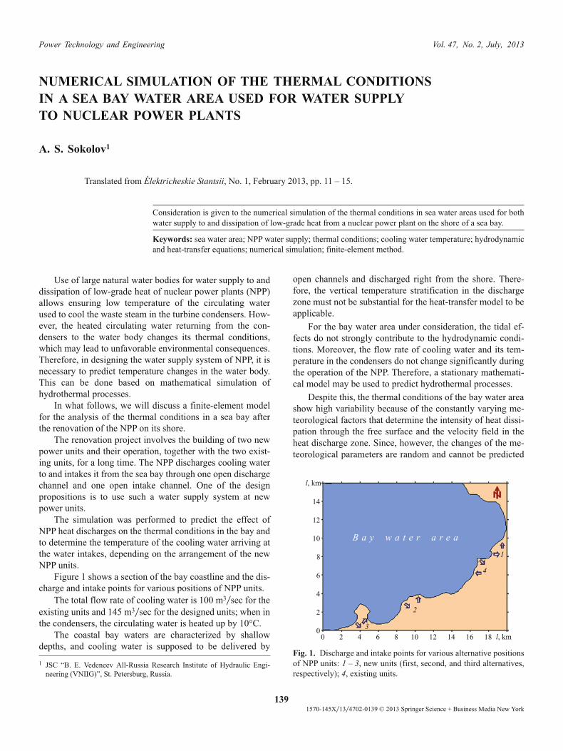
Figure 1 shows a section of the bay coastline and the dis-

charge and intake points for various positions of NPP units.

The total flow rate of cooling water is 100 m3�sec for the

existing units and 145 m3�sec for the designed units; when in

the condensers, the circulating water is heated up by 10°C.

The coastal bay waters are characterized by shallow

depths, and cooling water is supposed to be delivered by

open channels and discharged right from the shore. There-

fore, the vertical temperature stratification in the discharge

zone must not be substantial for the heat-transfer model to be

applicable.

For the bay water area under consideration, the tidal ef-

fects do not strongly contribute to the hydrodynamic condi-

tions. Moreover, the flow rate of cooling water and its tem-

perature in the condensers do not change significantly during

the operation of the NPP. Therefore, a stationary mathemati-

cal model may be used to predict hydrothermal processes.

Despite this, the thermal conditions of the bay water area

show high variability because of the constantly varying me-

teorological factors that determine the intensity of heat dissi-

pation through the free surface and the velocity field in the

heat discharge zone. Since, however, the changes of the me-

teorological parameters are random and cannot be predicted

Power Technology and Engineering Vol. 47, No. 2, July, 2013

139

1570-145X�13�4702-0139 © 2013 Springer Science + Business Media New York

1 JSC “B. E. Vedeneev All-Russia Research Institute of Hydraulic Engi-

neering (VNIIG)”, St. Petersburg, Russia.

14

12

10

8

6

4

2

00 2 4 6 8 10 12 14 16 18

l, km

l, km

B a y w a t e r a r e a

3

2

4

1

Fig. 1. Discharge and intake points for various alternative positions

of NPP units: 1 – 3, new units (first, second, and third alternatives,

respectively); 4, existing units.

over long periods, the effect of heat discharge of the NPP on

the thermal conditions of water bodies is usually evaluated

for some typical constant weather conditions.

The hydrothermal model used here is based on a system

of equations derived by integrating the three-dimensional hy-

drodynamic and heat-transfer equations with respect to the

vertical coordinate:

1 1

1

1 1 2

1

)

0 0 1

*

*

�

�

�

�

�

�

�

�

� �

*

*

� � � �

*

*

*

x

q q

HgH

xfq

x

q

i

i

s b

i*x

i

; (1)

1 2

2

2 2 1

2

)

0 0 1

*

*

�

�

�

�

�

�

�

�

� �

*

*

� � � �

*

*

*

x

q q

HgH

xfq

x

q

i

i

s b

i*x

i

; (2)

*

*

�

q

x

i

i

0; (3)

1

*

*

�

*

*

*

*

�

( ),

q T

x xa H

T

x c

i

i i

i

i

s2

(4)

where i = 1, 2, and summation is over repeated indices;

q v dxi i

h

�

�

�

)

3are the components of mass flow rate; x

iare

right-angle coordinates, x3

being the coordinate running

along the vertical axis directed upward; v1

and v2

are the

horizontal velocity components; ñ is the density of water

assumed constant; H = h + ç is the depth of water; h is the

depth measured from the reference surface x3

= 0 (free sur-

face at rest); ç is the elevation of the free surface; g is the

acceleration of gravity; ôsi

and ôbi

are the components of vis-

cous stress on the free surface and at the bottom; f is the

Coriolis parameter; . is the coefficient of viscosity; T is the

temperature of water; ai are the components of the heat-

transfer coefficient; Ös

is the heat-flow density on the free

surface; c is the specific heat of water.

Since the density of water is assumed constant, the equa-

tions of motion (1) – (3) can be solved independently of the

heat-transfer Eq. (4).

The components of viscous stress appearing in (1) – (2)

are defined by the formulas

0 1

s f ac W

1

2� cos ; (5)

0 1

s f ac W

2

2� sin ; (6)

0

b

g

C H

q q q1 2 2 1 1

2

2

2� � ; (7)

0

b

g

C H

q q q2 2 2 2 1

2

2

2� � , (8)

where cfis the wind stress coefficient; ñ

ais the density of air;

W is the wind velocity; è is the angle between the wind direc-

tion and the x1

axis; C is the Chezy coefficient.

The heat-flow density on the free surface can be found as

recommended in [1].

The variable T in (4) is the depth-average water tempera-

ture, while the formulas for Ös

include the water temperature

at the free surface. Therefore, to allow for the vertical tem-

perature stratification, it is necessary to relate these tempera-

tures based on the set vertical temperature profile.

In our case, the vertical variations in temperature may

be neglected as small and insignificant for the evaluation

of the effect of NPP discharges on the thermal conditions of

the bay.

The system of equations (1) – (4) should be supple-

mented with boundary conditions, formulating which for the

equations of motion involves some difficulties partially asso-

ciated with the incomplete validation of problem formula-

tions related to the integration of hydrodynamic equations,

despite the serious analytical studies in this area (see [2 –

6, etc.]).

Moreover, the information on the behavior of the un-

known functions on the boundary of the calculation domain

is in many cases insufficient to formulate boundary condi-

tions that would ensure the existence and uniqueness of the

solution.

In modeling coastal sea areas, for example, use is made

of an artificial liquid boundary separating the domain of in-

terest (open sea boundary). On this boundary, not only the

values of the hydrodynamic quantities are usually unknown,

but also the direction of current. The number of boundary

conditions that should be set to ensure the correctness of the

problem formulation may depend on the direction of water

movement through the boundary.

In [6] it is shown that if the viscosity terms are excluded

from Eqs. (1) and (2) in modeling tranquil flows, then two

boundary conditions should be set on the section of the liquid

boundary through which water enters the calculation domain

and one boundary condition on the section through which

water exits it. These boundary conditions cannot be arbitrary.

If Eqs. (1) and (2) include the viscosity terms, the num-

ber of boundary conditions on the liquid boundary should be

increased, which complicates the problem.

Therefore, boundary conditions are often set proceeding

from an “engineering” problem formulation and using

heuristic models of physical processes. In this connection,

of particular value are full-scale measurements that can be

used to calibrate (identify) the model and validate the results

of modeling.

One of the ways to resolve the problem of boundary con-

ditions for the hydrodynamic equations is to choose the cal-

culation domain so that the open sea boundary is so far from

the discharge and intake points that the effect of the bound-

ary conditions on the hydrothermal conditions in the dis-

charge zone is insignificant. Then boundary conditions may

be chosen somewhat arbitrarily. Thus, the size of the calcula-

tion domain can be found from numerical experiments.

140 A. S. Sokolov

The boundary conditions on the open sea boundary and

at the discharge and intake points are the following:

q qn n�

*; (9)

q q0 0

�

*,(10)

where qn

and qô are the normal and tangential (to the bound-

ary) components of the mass flow rate; qn

*and q

0

*are given

values.

Moreover, the following boundary condition is set on the

boundary sections through which water enters the calculation

domain:

ç = 0. (11)

It can be interpreted as attaching an infinitely deep reser-

voir with calm surface.

The following no-flow condition is set on the solid

(coastline) sections of the boundary:

qn = 0. (12)

Unlike the hydrodynamic problem, the mathematical for-

mulation of the heat-transfer problem based on Eq. (4) pres-

ents no special difficulties, though boundary conditions

should be prescribed accurately as well.

If intake water is of natural temperature Tn, which is typi-

cal for direct-flow water supply, the temperature of discharge

water can be defined as

Tdis = Tn + ÄT, (13)

where ÄT is the known increment in the temperature of the

cooling water in the condensers.

However, it is well to bear in mind that if the distance be-

tween the discharge and intake facilities is small and there is

no training wall between them, the temperature Tint

of intake

water may appear higher than Tn

because of the recirculation

of some discharge water to the intake and the diffusion trans-

fer of heat. Setting the boundary conditions (13) leads to an

incorrect solution of the problem because the amount of heat

discharged into sea, which is directly proportional to the dif-

ference of Tdis

and Tint

, is underestimated. To exclude miscal-

culation, the boundary conditions at the discharge point

should be as follows:

Tdis = Tint + ÄT, (14)

where Tdis

and Tint

are unknown.

The boundary conditions on the boundary sections

through which diffusion heat transfer can be neglected usu-

ally have the form

*

*

�

T

n0, (15)

where n is the normal coordinate to the boundary.

In the case being considered, such sections are the solid

coastline, the open sea boundary, and the intake points.

The following condition rather than (15) is set on the

section of the open sea boundary through which water enters

the calculation domain from the bay water area:

T = Tn. (16)

We use the finite-element method in combination with

the Galerkin method (see, e.g., [7 – 9]) for the numerical

simulation of hydrothermal processes. The numerical model

is based on simplex elements, i.e., the unknown functions are

approximated by polynomials containing a constant and

linear terms. To discretize the nonlinear terms in the mo-

mentum equations, use is made of the group finite-element

method [10].

The system of nonlinear algebraic equations derived by

applying the Galerkin method to the hydrodynamic equa-

tions is solved by Newton’s method.

The initial approximation is the values of the mass flow

rate obtained by using a simplified hydrodynamic model

based on the solution to the equation for the flow function

[11]. The values of qi for the open sea boundary are substi-

tuted into the boundary conditions (9) – (10). In the simpli-

fied hydrodynamic model, the flow function distribution on

the open sea boundary allows for the wind direction and av-

erage current in the bay used in the numerical experiment.

The numerical model is calibrated based on full-scale

measurements of the temperature in the coastal bay waters

during the operation of the NPP units.

Calculations are conducted using the average annual

weather conditions for the warmest month of the year and

various wind directions. The natural temperature Tn

cal-

culated using monthly average meteorological parameters

is 19.7°C.

The effect of NPP heat discharges on the thermal condi-

tions of the bay is assessed as the water area where the natu-

ral temperature is exceeded by more than 5°C. According to

fisheries regulations, such an increase in temperature is un-

acceptable, beginning from the control section.

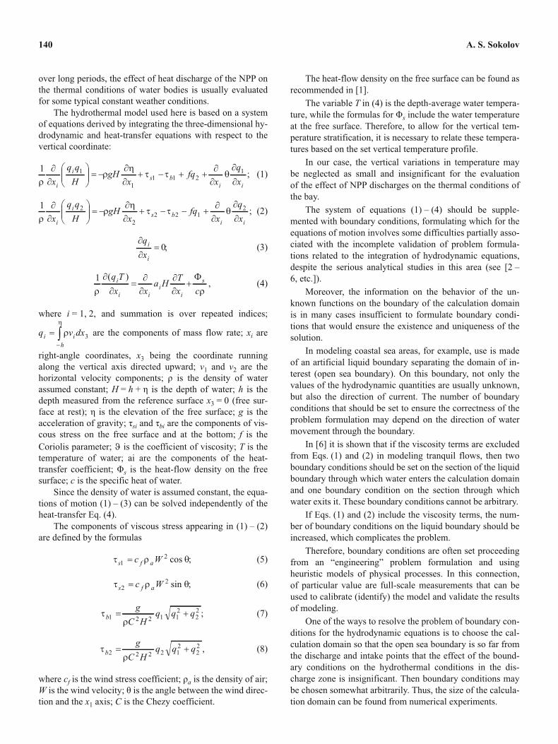
Figure 2 shows the calculated temperature fields for vari-

ous positions of new NPP units for numerical experiments in

which the bay water area where the natural temperature is

exceeded by more than 5°C appeared maximum. In this case,

such areas (obtained for different wind directions) differ in-

significantly. On the whole, however, numerical experiments

reveal that the water area where the natural temperature is

exceeded by more than 5°C increases with the distance be-

tween discharge points.

Calculations also show that the higher the temperature of

the discharged water and, hence, the higher the water temper-

ature in the discharge zone, the smaller the water area where

the natural temperature Tn

is exceeded. This is because, on

the one hand, heat dissipation through the free surface in-

creases with temperature and, on the other hand, the total

heat transferred to the atmosphere is invariant since, in

Numerical Simulation of the Thermal Conditions in a Sea Bay Water Area 141

steady-state conditions, it is always equal to the heat dis-

charged into the water body.

For example, the water areas where the natural tempera-

ture is exceeded by more than 5°C are maximum for the third

alternative arrangement of NPP units, while the temperatures

of discharge and intake water are minimum in this case. The

water area with excess of natural temperature by more than

5°C is minimum for the first alternative arrangement of NPP

units, while the temperatures of cooling water are maximum

in this case.

Numerical experiments show that for the second and

third alternative positions of new NPP units, the optimal (for

the condensers) direct-flow water supply at which the tem-

perature of intake water is equal to the natural temperature is

achieved only with certain wind directions. The maximum

excess of Tint

over Tn

for these alternatives is almost 5°C. For

the first alternative in which the existing and designed dis-

charge and intake facilities are closest to each other, the tem-

perature of cooling water is higher than the natural tempera-

ture, and its maximum excess over Tn

is 6.5°C for each wind

direction.

CONCLUSIONS

1. A numerical finite-element model for predicting the

thermal conditions of coastal sea waters used as a source of

cooling water for an NPP has been developed.

2. In the numerical simulation of heat transfer in sea wa-

ters, special attention should be given to the selection of the

calculation domain and the formulation of boundary condi-

tions.

3. To improve the numerical results, it is expedient to

use full-scale measurements for the calibration (identifica-

tion) of the model.

REFERENCES

1. Regulating Document RD 153-34.2-21.144–2003. Technologi-

cal Design of Cooling Water Reservoirs: Methodical Guidelines

[in Russian], Izd. VNIIG im. B. E. Vedeneeva, St. Petersburg

(2004).

2. N. E. Vol’tsinger and R. V. Pyaskovskii, Basic Oceanologic

Problems in Shallow-Water Theory [in Russian], Gidrometeoiz-

dat, Leningrad (1968).

3. O. A. Ladyzhenskaya, Mathematical Problems in the Dynamics

of Viscous Incompressible Fluid [in Russian], Nauka, Moscow

(1970).

4. R. Temam, Navier-Stokes Equations. Theory and Numerical

Analysis, North-Holland, Amsterdam (1977).

5. R. Peyret and T. D. Taylor, Computational Methods for Fluid

Flow, Springer Verlag, Berlin – Heidelberg – New York (1982).

6. V. F. Baklanovskaya, B. V. Pal’tsev, and I. I. Chechel’, “Bound-

ary-value problems for a system of Saint-Venant equations on a

plane,” Zh. Vych. Mat. Mat. Fiz., 19(3), 708 – 725 (1979).

7. L. J. Segerlind, Applied Finite Element Analysis, John Wiley &

Sons, New York (1976).

8. J. J. Connor and C. A. Brebbia, Finite Element Techniques for

Fluid Flow, Newnes-Butterworth, London (1976).

9. C. A. J. Fletcher, Computational Galerkin Methods, Springer

Verlag, New York (1984).

10. C. A. J. Fletcher, Computational Techniques for Fluid Dynam-

ics. Vol. 1, Springer Verlag, Berlin (1987).

11. I. I. Makarov, A. S. Sokolov, and S. G. Shul’man, Modeling

Hydrothermal Processes in Cooling Water Reservoirs [in Rus-

sian], Énergoatomizdat, Moscow (1986).

142 A. S. Sokolov

14

14

14

12

12

12

10

10

10

8

8

8

6

6

6

4

4

4

2

2

2

0

0

0

0

0

0

2

2

2

4

4

4

6

6

6

8

8

8

10

10

10

12

12

12

14

14

14

16

16

16

18

18

18

l, km

l, km

l, km

l, km

l, km

l, km

36

36

36

35

35

35

34

34

34

33

33

33

32

32

32

31

31

31

30

30

30

29

29

29

28

28

28

27

27

27

26

26

26

25

25

25

24

24

24

23

23

23

22

22

22

21

21

21

20

20

20

19

19

19

°C

°C

°C

a

b

c

B a y w a t e r a r e a

B a y w a t e r a r e a

B a y w a t e r a r e a

Fig. 2. Temperature fields for various alternative positions of NPP

units: a, first alternative and northwest; b, second alternative and

north; c, third alternative and southwest.