Acta Mech 230, 667–682 (2019)https://doi.org/10.1007/s00707-018-2265-5

ORIGINAL PAPER

Marco E. Rosti · Francesco De Vita · Luca Brandt

Numerical simulations of emulsions in shear flows

Received: 14 March 2018 / Revised: 14 May 2018 / Published online: 13 October 2018© The Author(s) 2018

Abstract We present a modification of a recently developed volume of fluid method for multiphase problems(Ii et al. in J Comput Phys 231(5):2328–2358, 2012), so that it can be used in conjunction with a fractional-step method and fast Poisson solver, and validate it with standard benchmark problems. We then consideremulsions of two-fluid systems and study their rheology in a plane Couette flow in the limit of vanishinginertia. We examine the dependency of the effective viscosity μ on the volume fraction Φ (from 10 to 30%)and the Capillary number Ca (from 0.1 to 0.4) for the case of density and viscosity ratio 1. We show that theeffective viscosity decreases with the deformation and the applied shear (shear-thinning) while exhibiting anon-monotonic behavior with respect to the volume fraction. We report the appearance of a maximum in theeffective viscosity curve and compare the results with those of suspensions of rigid and deformable particlesand capsules. We show that the flow in the solvent is mostly a shear flow, while it is mostly rotational inthe suspended phase; moreover, this behavior tends to reverse as the volume fraction increases. Finally, weevaluate the contributions to the total shear stress of the viscous stresses in the two fluids and of the interfacialforce between them.

1 Introduction

In the last decades, developments in colloidal science have proven to be crucial for fabrication of functionalmaterials. Particles or droplets, with typical scales of micron, are manipulated to self-organize into controlledpatterns with high precision, which then form basic building blocks for more complex structures [44]. Oneimportant aspect to consider during the synthesis and assembly of innovative materials is the rheologicalbehavior of the system [29]. Indeed, the material properties will depend on the distribution of the dispersedphase, and thus, a more accurate control of the production process can help to generate materials of desiredproperties [58].

A great amount of work has been done in the past to study rigid and deformable particle suspensions[1,18,41,42,51]. In his pioneering work, Einstein [15] showed that, in the limit of vanishing inertia and fordilute rigid particle suspensions, the viscosity is a linear function of the particle volume fraction. AlthoughBatchelor and Green [4] and Batchelor [3] added a second-order correction, all existing analytical relationsare not valid for moderately high concentrations and one needs to resort to empirical fits. One of the availableempirical relations that provides a good description of the rheology at zero Reynolds number both in the highand low concentration limits is the Eilers fit [16,23,48,64]. Recently, inertia and deformation have been shownto introduce deviations from the behavior predicted by the different empirical fits, and these effects can berelated to an increase and decrease of an effective volume fraction [31,42].

M. E. Rosti (B) · F. De Vita · L. BrandtLinné Flow Centre and SeRC, KTH Mechanics, Stockholm, SwedenE-mail: merosti@mech.kth.se

668 M. E. Rosti et al.

Less attention has been given to emulsions, which are instead the object of the present work. Emulsionsare biphasic liquid–liquid systems in which the phases are separated by a deformable interface subject tointerfacial surface tension. These can be found in a variety of applications, ranging from advanced materialsprocessing, waste treatment, enhanced oil recovery, food processing to pharmaceutical manufacturing. Simi-larly to particle suspensions, it is often desirable to predict or manipulate the rheology and microstructure ofemulsions, which in general exhibit highly varied rheological behaviors [27]; however, there has been limitedprogress toward the creation of theoretical models that can reliably predict the rheology and microstructureof such flows [25,26], and for years measurements of emulsion rheology were not quantitatively understoodbecause of the complexity of the phenomenology involved and the difficulty to properly choose materialswith controlled properties [27]. Thus, numerical simulations can help to fill this gap, and indeed there hasbeen considerable progress in the development of numerical simulations able to study such multiphase flows[36,56].

Different techniques have been proposed to numerically tackle the problem at hand. The so-called front-tracking method is an Eulerian/Lagrangian method, used to simulate viscous, incompressible, immiscibletwo-fluid systems, first developed by Unverdi and Tryggvason [57] and Tryggvason et al. [54]. When dealingwith moving and deformable boundaries, an alternative approach are the so-called front-capturing methods,which are fully Eulerian and handle topology changes automatically. A strong advantage of these methods isthat they are easier to parallelize than their Lagrangian counterpart. Eulerian interface representations includeessentially the volume of fluid (VOF) [45] and level-set (LS) [46,47,50] methods. The volume of fluid methoddefines different fluids with a discontinuous color function, and its main advantage is the intrinsic massconservation; however, it suffers from an inaccurate computation of the interface properties, such as normalsand curvatures [10,17]. Differently from the volume of fluid, the level-set method prescribes the interface bya continuous function which usually takes the form of the signed distance to the interface. Thus, normals andcurvatures can be readily and accurately computed, while mass loss or gain may occur. In this work, we willemploy the volume of fluid method.

In a conventional VOF method, the interface separating different fluids is piece-wisely reconstructed ineach numerical cell by straight line segments, which are then used to calculate the numerical fluxes necessary toupdate the local volume of fluid function. This geometric reconstruction effectively eliminates the numericaldiffusion that smears out the compactness of the transition layer of the interface. Different methodologieshave been proposed to accurately recover the exact surface geometry from the discretized VOF function:the simple line interface calculation (SLIC) method [30] and the piecewise linear interface calculation (PLIC)[61,62], the latter being furthermodified by several authors [2,19,33,37,39].Another technique is the tangent ofhyperbola for interface capturing (THINC) method [59], which avoids the explicit geometric reconstruction byusing a continuous sigmoid function rather than the Heaviside function, thus allowing a completely algebraicdescription of the interface; this enables the computation of the numerical flux partially analytically. Animprovementwas proposed by combining the original THINCmethodwith the first-order upwind scheme in theso-called THINC/WLIC (THINC/weighted linear interface capturing) method [60]. Recently, the method hasbeen further developed in themulti-dimensional THINC (MTHINC)methodwhere the fullymulti-dimensionalhyperbolic tangent function is used to reconstruct the interface [21]. The numerical fluxes can be directlyevaluated by integrating the hyperbolic tangent function, and the normal vector, curvature, and approximatedelta function can be directly obtained from the derivatives of the function. Moreover, the scheme does notrequire the geometric reconstruction, and a curved (quadratic) surface can be easily constructed as well.

1.1 Outline

In this work, we first present our numerical solver for multiphase incompressible flows and then employ it tostudy liquid–liquid systems (emulsions) in a plane Couette flow at low Reynolds number. The two fluids areNewtonian and satisfy the full incompressible Navier–Stokes equations. We compare our results with those ofsuspensions of rigid and deformable particles and with capsules, consisting of a second fluid enclosed by a thinelastic membrane. In Sect. 2, we first discuss the flow configuration and governing equations, and then presentthe numerical methodology used and its validation. The rheological study of the emulsions is presented inSect. 3, where we also discuss the role of the different non-dimensional parameters governing the flow. Finally,a summary of the main findings and some conclusions are drawn in Sect. 4.

Numerical simulations of emulsions in shear flows 669

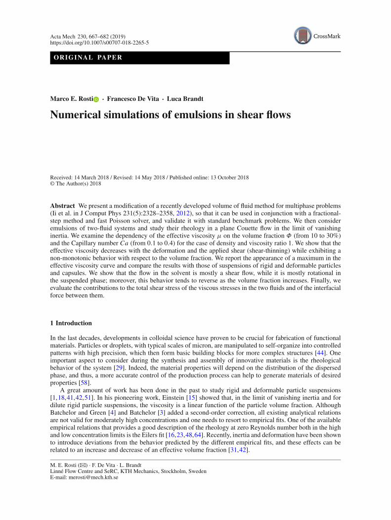
Fig. 1 Sketch of the channel geometry and coordinate system adopted in this study

2 Formulation

We consider the flow of two incompressible viscous fluids, separated by an interface, in a channel with movingwalls, i.e., in a plane Couette geometry. Figure 1 shows a sketch of the geometry and the Cartesian coordinatesystem, where x , y, and z (x1, x2, and x3) denote the streamwise, wall-normal, and spanwise coordinates,while u, v, andw (u1, u2, and u3) denote the corresponding components of the velocity vector field. The lowerand upper impermeable moving walls are located at y = −h and y = h, respectively, and move in oppositedirection with constant streamwise velocity ± Vw.

The two-fluid motion is governed by the conservation of momentum and the incompressibility constraint,and the kinematic and dynamic interactions between the two fluid phases are determined by enforcing thecontinuity of the velocity and traction force at the interface between the two phases, i.e.,

u f 1i = u f 2

i and σf 1i j n j = σ

f 2i j n j + σκni , (1)

where the suffixes f 1 and f 2 are used to indicate the two phases, σi j denotes the Cauchy stress tensor, nithe normal vector at the interface, κ the interface curvature, and σ the surface tension (assumed here to beconstant).

To numerically solve the two-phase interaction problem at hand, we use the volume of fluid methodfollowing Ii et al. [21]. We introduce an indicator (or color) function H to identify each fluid phase so thatH = 1 in the region occupied by the fluid f 1 and H = 0 otherwise. Considering that the fluid is transportedby the flow velocity, we update H in the Eulerian framework by the following advection equation written indivergence form:

∂φ

∂t+ ∂ui H

∂xi= φ

∂ui∂xi

(2)

where ui is the local fluid velocity and φ the cell-averaged value of the indicator function.Once φ is known, the two-fluid equations can be rewritten in the so-called one-continuum formulation [55],

so that only one set of equations is solved over the whole domain. This is achieved by introducing a monolithicvelocity vector field ui , defined everywhere and found by applying the volume averaging procedure [38,52].Thus, ui is governed by the following set of equations:

∂ui∂t

+ ∂uiu j

∂x j= 1

ρ

(∂σi j

∂x j+ fi

), (3.1)

∂ui∂xi

= 0 (3.2)

where ρ is the density, fi the surface tension force defined as fi = σκniδ, being δ the delta function at theinterface, and σi j is the stress written in a mixture form, i.e.,

σi j = (1 − φ) σf 1i j + φσ

f 2i j . (4)

Note that we have chosen φ to be the volume fraction of fluid 2, i.e., this is zero in the fluid 1, whereas φ = 1in the fluid 2, and 0 ≤ φ ≤ 1 close to the interface. Both fluids are assumed to be Newtonian so that theirstress tensors can be written as σi j = −pδi j + 2μDi j , where p is the pressure, δi j the Kronecker delta, μ

670 M. E. Rosti et al.

the dynamic viscosity, and Di j the strain rate tensor (defined as Di j = (∂ui/∂x j + ∂u j/∂xi )/2). Finally, themixture density ρ and dynamic viscosity μ are simply averaged in terms of the local φ:

ρ = (1 − φ) ρ f 1 + φρ f 2 and μ = (1 − φ) μ f 1 + φμ f 2. (5)

Note that, in order to solve Eqs. (3.1) and (2), we need to determine the indicator function H , the normal vectorni , and the curvature κ .

2.1 The MTHINC method

The indicator function H can be reconstructed in various ways; here, we use the multi-dimensional tangent ofhyperbola for interface capturing (MTHINC) method, developed by Ii et al. [21], where a multi-dimensionalhyperbolic tangent function is used as an approximated indicator function. In particular, the indicator functionH is approximated as

H (X, Y, Z) ≈ H (X, Y, Z) = 1

2

(1 + tanh

(β (P (X, Y, Z) + d)

))(6)

where X, Y, Z ∈ [0, 1] is a centered local coordinate system defined in each cell, P is a three-dimensionalsurface function, β a sharpness parameter, and d a normalization parameter. The function P can be either alinear function (a plane)

P (X, Y, Z) = a100X + a010Y + a001Z (7)

or a quadratic function (a curved surface)

P (X, Y, Z) = a200X2 + a020Y

2 + a002Z2

+ a110XY + a011Y Z + a101X Z + a100X + a010Y + a001Z .(8)

The coefficients al,m,n are determined algebraically by imposing the correct value of the three normal com-ponents ni and the six components of the Cartesian curvature tensor li j = (

∂ni/∂x j + ∂n j/∂xi)/2 for the

function P in each cell. Finally, the parameter d is found by enforcing the following constraint:

∫ 1

0

∫ 1

0

∫ 1

0H dX dY dZ = φ. (9)

The integration can be performed analytically in one direction, and numerically in the other two directions bythe two-point Gaussian quadrature.

The unit normal vector is defined as ni = mi/|∇φ|, being mi the gradient of the volume of fluid function,i.e., mi = ∂φ/∂xi . Here, we compute mi using the usual Youngs’ approach [61,62], where first the valuesof the derivative at the cell corners are calculated, and then averaged to find the cell-center value. Once thenormal vector is known, the curvature κ can be easily found by taking the divergence of the normal vector,i.e., κ = −∂ni/∂xi , and the surface tension force fi can be computed by the continuum surface force (CSF)model [5], where the 1D approximate delta function δ is directly approximated by δ ≈ |∇φ|. Thus, we obtain

fi = σκniδ ≈ σκ∂φ

∂xi. (10)

2.2 Numerical discretization

The equation of motion is solved with an extensively validated in-house code [32,40–42]. The equations aresolved on a staggered uniform grid with velocities located on the cell faces and all the other variables (pressure,stress, and volume of fluid) at the cell centers. All the spatial derivatives are approximated with second-ordercentered finite differences, while the time integration is discussed hereafter.

First, the volume of fluid function is updated in time from the time step (n) to (n + 1) by solving Eq. (2),following the procedure proposed by Ii et al. [21]. In particular, the time evolution of φ is calculated by

Numerical simulations of emulsions in shear flows 671

evaluating the numerical fluxes sequentially in each direction, a robust and easy approach called directionalsplitting. Thus, Eq. (2) is discretized sequentially in the three Cartesian direction, i.e.,

φi jk(∗) = φ(n) − 1

x

(fi+ 1

2 , j,k(n) − f

i− 12 , j,k

(n)

)+ t

xφi, j,k(∗)

(ui+ 1

2 , j,k1 − u

i− 12 , j,k

1

),

φi jk(∗∗) = φ(∗) − 1

x

(gi, j+ 1

2 ,k(∗) − g

i, j− 12 ,k

(∗)

)+ t

xφi, j,k(∗∗)

(ui, j+ 1

2 ,k2 − u

i, j− 12 ,k

2

),

φi jk(∗∗∗) = φ(∗∗) − 1

x

(hi, j,k+ 1

2(∗∗) − h

i, j,k− 12

(∗∗)

)+ t

xφi, j,k(∗∗∗)

(ui, j,k+ 1

23 − u

i, j,k− 12

3

)(11)

where the subscript in parenthesis indicates the time iteration, with (n) and (n+1) the old and new time steps,and (∗), (∗∗), and (∗ ∗ ∗) sub-iterations. Also, t = t(n+1) − t(n) is the time step, and f , g, and h are thenumerical fluxes defined later on. Note that Eq. (11) is implicit in the function φ in each sub-step. Next, wesolve an additional equation in order to ensure the divergence-free condition of the fully multi-dimensionaloperator [2,37]:

φi jk(n+1) = φ(∗∗∗) − t

(φi jk(∗)

ui+ 1

2 , j,k1 − u

i− 12 , j,k

1

x+ φ

i jk(∗∗)

ui, j+ 1

2 ,k2 − u

i, j− 12 ,k

2

y

+ φi jk(∗∗∗)

ui, j,k+ 1

23 − u

i, j,k− 12

3

z

).

(12)

Finally, we need to specify how the numerical fluxes are treated. These are defined as the space/time integrationof the product of the velocityui and the indicator function H ,which is substituted by its approximate counterpartH , i.e.,

fi± 1

2 , j,k(n) = 1

yz

∫δt(n)

∫y

∫z

(u1 H

)i± 12 , j,k

dy dz dt,

gi, j± 1

2 ,k(∗) = 1

xz

∫δt(∗)

∫x

∫z

(u2 H

)i, j± 12 ,k

dx dz dt,

hi, j,k± 1

2(∗∗) = 1

xy

∫δt(∗∗)

∫x

∫y

(u3 H

)i, j,k± 12 dx dy dt.

(13)

The temporal integration can be replaced by a spatial integration along the upwind path on the velocity field.

For example, in the x-direction the upstream path is x+ =[xi+ 1

2 − tui+ 12 , j,k, xi+ 1

2

]for u

i+ 12

1 ≥ 0 or

x− =[xi+ 1

2 , xi+ 12 − tui+ 1

2 , j,k]for u

i+ 12

1 < 0. A similar procedure is applied in the other two coordinate

directions. Thus, the numerical fluxes can be computed as

fi+ 1

2 , j,k(n) =

⎧⎨⎩

1yz

∫x+

∫y

∫z H

i, j,k(n) dx dy dz for u

i+ 12 , j,k

1 ≥ 0

− 1yz

∫x−

∫y

∫z H

i+1, j,k(n) dx dy dz for u

i+ 12 , j,k

1 < 0,

gi, j+ 1

2 ,k(∗) =

⎧⎨⎩

1xz

∫x

∫y+

∫z H

i, j,k(∗) dx dy dz for u

i, j+ 12 ,k

2 ≥ 0

− 1xz

∫x

∫y−

∫z H

i, j+1,k(∗) dx dy dz for u

i, j+ 12 ,k

2 < 0,

hi, j,k+ 1

2(∗∗) =

⎧⎨⎩

1xy

∫x

∫y

∫z+ H i, j,k

(∗∗) dx dy dz for ui, j,k+ 1

23 ≥ 0

− 1xy

∫x

∫y

∫z− H i, j,k+1

(∗∗) dx dy dz for ui, j,k+ 1

23 < 0.

(14)

Similarly to Eq. (9), the numerical integration can be performed analytically in one direction, and numericallyin the other two by the two-point Gaussian quadrature.

Once the volume of fluid function has been updated, i.e., φn+1 is available, differently from what done byIi et al. [21], the time integration of Eq. (3.1) is here performed with a fractional-step method [22] where theevolution equation is advanced in timewith a second-order Adam–Bashforth scheme, and a Fast Poisson Solver

672 M. E. Rosti et al.

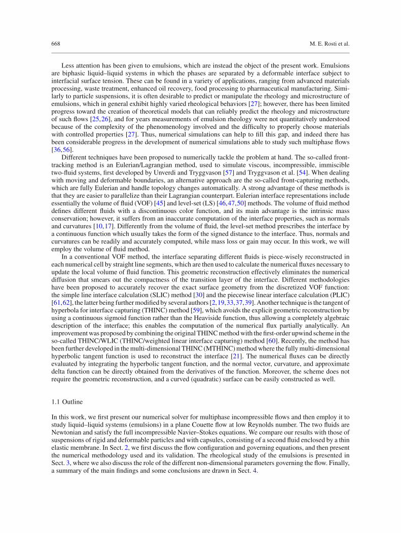
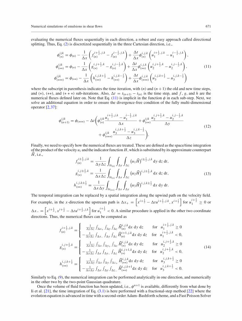
Fig. 2 The 2D Zalesak’s disk: simulation of a slotted disk undergoing solid body rotation [63]. The black line denotes the exactinitial solution, whereas blue and red the solutions obtained after one and five full revolutions. The two left figures are obtainedwith β = 1 and the two right ones with β = 2. In both sides, the results in the two panels are obtained with 33 and 66 grid pointsper diameter (color figure online)

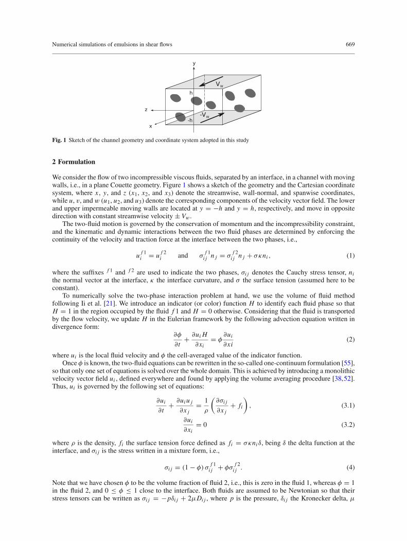
Fig. 3 The 3D Zalesak’s disk: the three panels represent the exact initial solution, and those after one full rotation with 33 and66 grid points per diameter

is used to enforce zero divergence of the velocity field. Due to the non-uniformity of the density, the Poissonequation used to enforce a divergence-free velocity field results in an equation with variable coefficients, i.e.,

∂

∂xi

(1

ρ

∂p

∂xi

)= 1

t

∂ ui∂xi

(15)

where the pressure p and density ρ are evaluated at n + 1 and the velocity ui is the non-divergence-freepredicted velocity. In order to employ an efficient FFT-based pressure solver with constant coefficients (seealso [12,13]), we use the following splitting of the pressure term [14]:

1

ρ

∂p

∂xi→ 1

ρ0

∂p

∂xi+

(1

ρ− 1

ρ0

)∂ p

∂xi(16)

where ρ0 is a constant density equal to the lowest density of the two phases, and p is an approximated pressureobtained by linear extrapolation, e.g., p = 2pn − pn−1. With this splitting, the Poisson equation can berewritten as

∂2 p

∂xi∂xi= ρ0

t

∂ ui∂xi

+ ∂

∂xi

[(1 − ρ0

ρ

)∂ p

∂xi

]. (17)

Note that also the correction step of the fractional-step method needs to be modified accordingly.

2.3 Code validation

The Zalesak’s disk [63], i.e., a slotted disk undergoing solid body rotation, is a standard benchmark to validatenumerical schemes for advection problems, since the initial shape should not deform under rigid body rotation.The setup is the same as described by Ii et al. [21], and the comparison of the initial shape (black line) andthose after one (blue line) and five (red line) full rotations is shown in Fig. 2. We consider two grid resolutionshere, 100 and 200 grid points per box size (being the disk of size 0.3), and two different values of the sharpnessparameter β: 1 and 2. The deformed shape of the disk shows an overall good agreement with the initial one,with the comparison deteriorating when more rotations are performed. Better agreement is found on the finergrid, and this is further slightly improved in the case with β = 2. As expected, the major differences are foundon the sharp edges of the geometry, which are difficult to maintain undeformed. The test has been repeatedin 3D, and the results are shown in Fig. 3. Again, quite good agreement is found between the initial and finalshapes, with the difference reducing with increasing resolution.

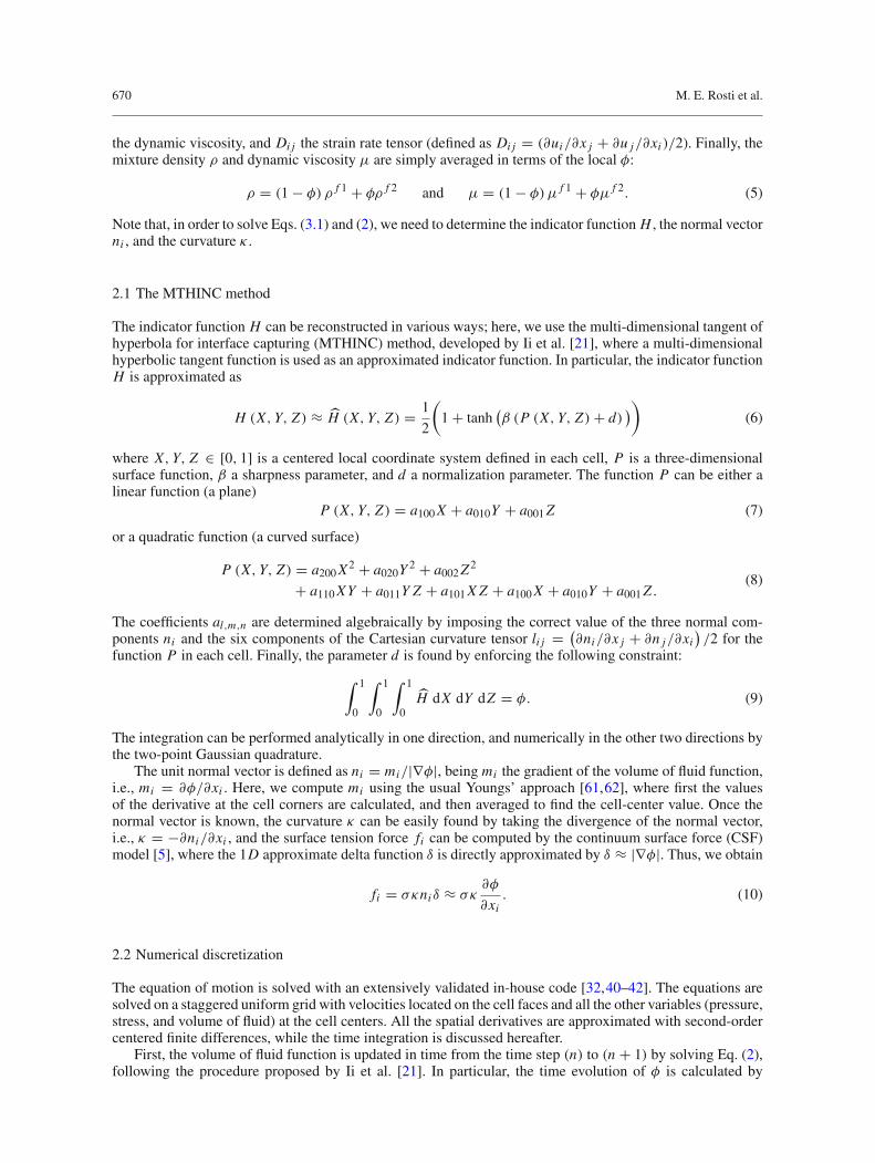
Next, we study a deformed interface in a shear flow in order to evaluate the capability of the methodto capture a heavily deformed and stretched interface [43]. We consider a circle of radius 0.2π , centered at[0.5π, −0.2(π + 1)] in a box of side 2π with the prescribed velocity field u1 = sin(x) cos(y) and u2 =

Numerical simulations of emulsions in shear flows 673

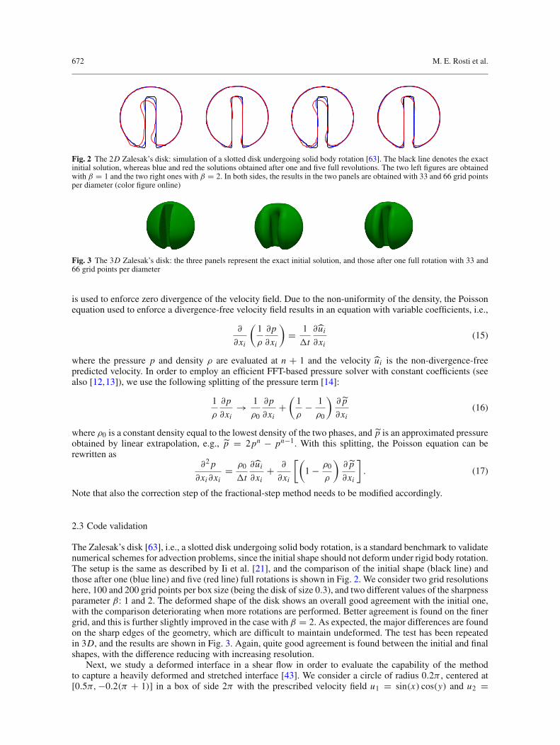
Fig. 4 A deformed interface in a shearing flow: the black, blue, and red lines denote the interface at t = 0, 5π and 10π ,respectively. The three panels are obtained with 100, 150, and 200 grid points per box side (color figure online)

−1

0

1

−1 0 1

y/D

x/D

0

1

0 1

t

(a) (b)

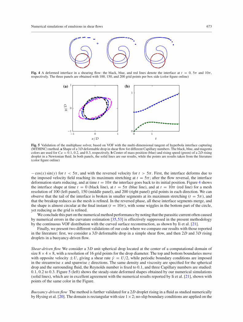
Fig. 5 Validation of the multiphase solver, based on VOF with the multi-dimensional tangent of hyperbola interface capturing(MTHINC) method. a Shape of a 3D deformable drop in shear flow for different Capillary numbers. The black, blue, andmagentacolors are used for Ca = 0.1, 0.2, and 0.3, respectively. b Center of mass position (blue) and rising speed (green) of a 2D risingdroplet in a Newtonian fluid. In both panels, the solid lines are our results, while the points are results taken from the literature(color figure online)

− cos(x) sin(y) for t < 5π , and with the reversed velocity for t > 5π . First, the interface deforms due tothe imposed velocity field reaching its maximum stretching at t = 5π ; after the flow reversal, the interfacedeformation starts reducing, and at time t = 10π the interface goes back to its initial position. Figure 4 showsthe interface shape at time t = 0 (black line), at t = 5π (blue line), and at t = 10π (red line) for a meshresolution of 100 (left panel), 150 (middle panel), and 200 (right panel) grid points in each direction. We canobserve that the tail of the interface is broken in smaller segments at its maximum stretching (t = 5π), andthat the breakup reduces as the mesh is refined. In the reversed phase, all these interface segments merge, andthe shape is almost circular at the final instant (t = 10π), with some wiggles in the bottom part of the circle,yet reducing as the grid is refined.

We conclude this part on the numericalmethod performance by noting that the parasitic current often causedby numerical errors in the curvature estimation [35,53] is effectively suppressed in the present methodologyby the continuous VOF distribution with the curved surface reconstruction, as shown by Ii et al. [21].

Finally, we present two different validations of our code where we compare our results with those reportedin the literature: first, we consider a 3D deformable drop in a simple shear flow, and then 2D and 3D risingdroplets in a buoyancy-driven flow.

Shear-driven flow We consider a 3D unit spherical drop located at the center of a computational domain ofsize 8× 4× 8, with a resolution of 16 grid points for the drop diameter. The top and bottom boundaries movewith opposite velocity ±U , giving a shear rate γ = U/2, while periodic boundary conditions are imposedin the streamwise x and spanwise z directions. The same density and viscosity are specified for the sphericaldrop and the surrounding fluid, the Reynolds number is fixed to 0.1, and three Capillary numbers are studied:0.1, 0.2 to 0.3. Figure 5 (left) shows the steady-state deformed shapes obtained by our numerical simulations(solid lines), which are in excellent agreement with the numerical results reported by Ii et al. [21], shown withpoints of the same color in the Figure.

Buoyancy-driven flow The method is further validated for a 2D droplet rising in a fluid as studied numericallyby Hysing et al. [20]. The domain is rectangular with size 1×2; no-slip boundary conditions are applied on the

674 M. E. Rosti et al.

0

0.5

1

0 0.5 1

uf1

y/h

0

0.2

0.4

0.6

0 0.5 1

φ

y/h

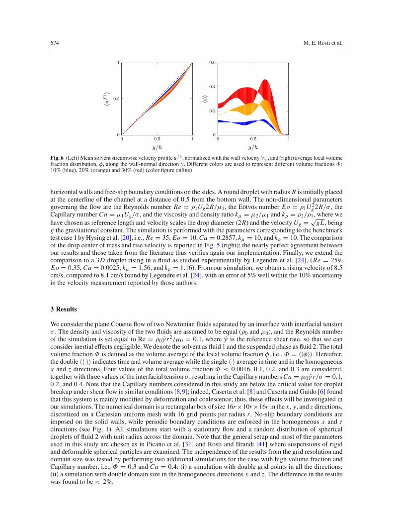
Fig. 6 (Left)Mean solvent streamwise velocity profile u f 1, normalizedwith thewall velocity Vw, and (right) average local volumefraction distribution, φ, along the wall-normal direction y. Different colors are used to represent different volume fractions Φ:10% (blue), 20% (orange) and 30% (red) (color figure online)

horizontal walls and free-slip boundary conditions on the sides. A round droplet with radius R is initially placedat the centerline of the channel at a distance of 0.5 from the bottom wall. The non-dimensional parametersgoverning the flow are the Reynolds number Re = ρ1Ug2R/μ1, the Eötvös number Eo = ρ1U 2

g2R/σ , theCapillary number Ca = μ1Ug/σ , and the viscosity and density ratio kμ = μ2/μ1 and kρ = ρ2/ρ1, where wehave chosen as reference length and velocity scales the drop diameter (2R) and the velocityUg = √

gL , beingg the gravitational constant. The simulation is performed with the parameters corresponding to the benchmarktest case 1 byHysing et al. [20], i.e., Re = 35, Eo = 10,Ca = 0.2857, kμ = 10, and kρ = 10. The comparisonof the drop center of mass and rise velocity is reported in Fig. 5 (right); the nearly perfect agreement betweenour results and those taken from the literature thus verifies again our implementation. Finally, we extend thecomparison to a 3D droplet rising in a fluid as studied experimentally by Legendre et al. [24], (Re = 259,Eo = 0.35, Ca = 0.0025, kμ = 1.56, and kρ = 1.16). From our simulation, we obtain a rising velocity of 8.5cm/s, compared to 8.1 cm/s found by Legendre et al. [24], with an error of 5% well within the 10% uncertaintyin the velocity measurement reported by those authors.

3 Results

We consider the plane Couette flow of two Newtonian fluids separated by an interface with interfacial tensionσ . The density and viscosity of the two fluids are assumed to be equal (ρ0 and μ0), and the Reynolds numberof the simulation is set equal to Re = ρ0γ r2/μ0 = 0.1, where γ is the reference shear rate, so that we canconsider inertial effects negligible.We denote the solvent as fluid 1 and the suspended phase as fluid 2. The totalvolume fraction Φ is defined as the volume average of the local volume fraction φ, i.e., Φ = 〈〈φ〉〉. Hereafter,the double 〈〈·〉〉 indicates time and volume average while the single 〈·〉 average in time and in the homogeneousx and z directions. Four values of the total volume fraction Φ ≈ 0.0016, 0.1, 0.2, and 0.3 are considered,together with three values of the interfacial tension σ , resulting in the Capillary numbersCa = μ0γ r/σ = 0.1,0.2, and 0.4. Note that the Capillary numbers considered in this study are below the critical value for dropletbreakup under shear flow in similar conditions [8,9]; indeed, Caserta et al. [8] and Caserta and Guido [6] foundthat this system is mainly modified by deformation and coalescence; thus, these effects will be investigated inour simulations. The numerical domain is a rectangular box of size 16r×10r×16r in the x , y, and z directions,discretized on a Cartesian uniform mesh with 16 grid points per radius r . No-slip boundary conditions areimposed on the solid walls, while periodic boundary conditions are enforced in the homogeneous x and zdirections (see Fig. 1). All simulations start with a stationary flow and a random distribution of sphericaldroplets of fluid 2 with unit radius across the domain. Note that the general setup and most of the parametersused in this study are chosen as in Picano et al. [31] and Rosti and Brandt [41] where suspensions of rigidand deformable spherical particles are examined. The independence of the results from the grid resolution anddomain size was tested by performing two additional simulations for the case with high volume fraction andCapillary number, i.e., Φ = 0.3 and Ca = 0.4: (i) a simulation with double grid points in all the directions;(ii) a simulation with double domain size in the homogeneous directions x and z. The difference in the resultswas found to be < 2%.

Numerical simulations of emulsions in shear flows 675

1

1.2

1.4

0 0.1 0.2 0.3

μ/μ0

Φ

1

2

3

0 50 100

μ/μ0

γt

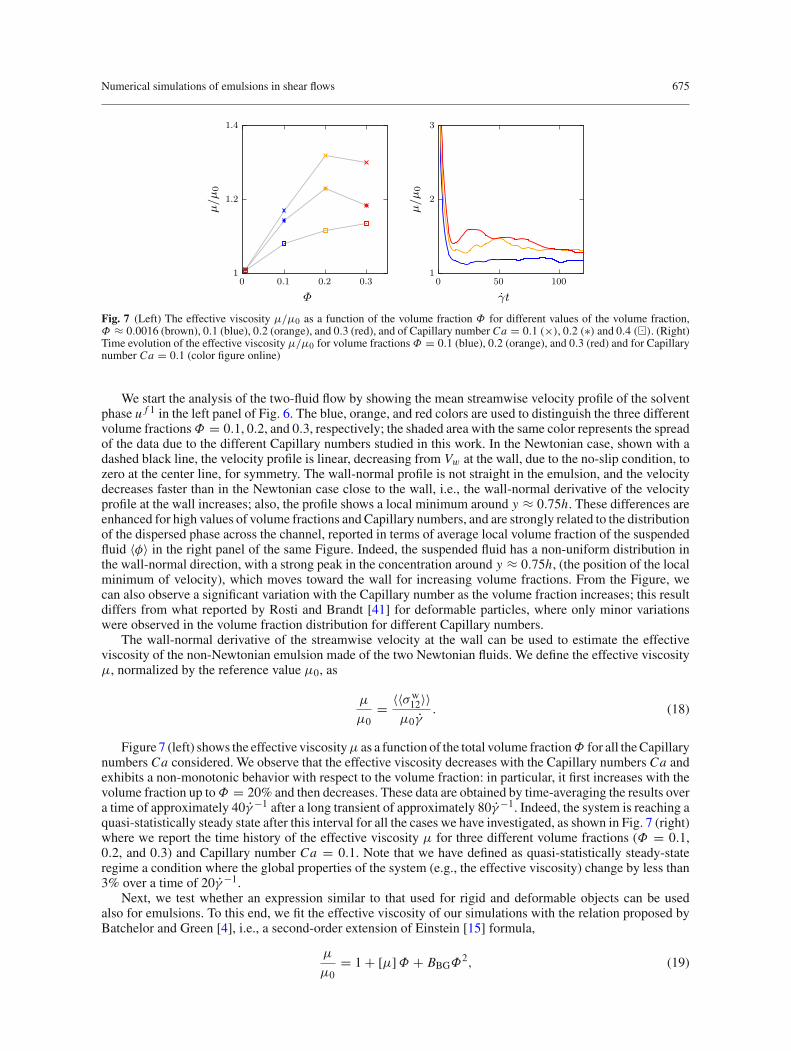
Fig. 7 (Left) The effective viscosity μ/μ0 as a function of the volume fraction Φ for different values of the volume fraction,Φ ≈ 0.0016 (brown), 0.1 (blue), 0.2 (orange), and 0.3 (red), and of Capillary number Ca = 0.1 (×), 0.2 (∗) and 0.4 (�). (Right)Time evolution of the effective viscosity μ/μ0 for volume fractions Φ = 0.1 (blue), 0.2 (orange), and 0.3 (red) and for Capillarynumber Ca = 0.1 (color figure online)

We start the analysis of the two-fluid flow by showing the mean streamwise velocity profile of the solventphase u f 1 in the left panel of Fig. 6. The blue, orange, and red colors are used to distinguish the three differentvolume fractionsΦ = 0.1, 0.2, and 0.3, respectively; the shaded area with the same color represents the spreadof the data due to the different Capillary numbers studied in this work. In the Newtonian case, shown with adashed black line, the velocity profile is linear, decreasing from Vw at the wall, due to the no-slip condition, tozero at the center line, for symmetry. The wall-normal profile is not straight in the emulsion, and the velocitydecreases faster than in the Newtonian case close to the wall, i.e., the wall-normal derivative of the velocityprofile at the wall increases; also, the profile shows a local minimum around y ≈ 0.75h. These differences areenhanced for high values of volume fractions and Capillary numbers, and are strongly related to the distributionof the dispersed phase across the channel, reported in terms of average local volume fraction of the suspendedfluid 〈φ〉 in the right panel of the same Figure. Indeed, the suspended fluid has a non-uniform distribution inthe wall-normal direction, with a strong peak in the concentration around y ≈ 0.75h, (the position of the localminimum of velocity), which moves toward the wall for increasing volume fractions. From the Figure, wecan also observe a significant variation with the Capillary number as the volume fraction increases; this resultdiffers from what reported by Rosti and Brandt [41] for deformable particles, where only minor variationswere observed in the volume fraction distribution for different Capillary numbers.

The wall-normal derivative of the streamwise velocity at the wall can be used to estimate the effectiveviscosity of the non-Newtonian emulsion made of the two Newtonian fluids. We define the effective viscosityμ, normalized by the reference value μ0, as

μ

μ0= 〈〈σw

12〉〉μ0γ

. (18)

Figure 7 (left) shows the effective viscosityμ as a function of the total volume fractionΦ for all theCapillarynumbers Ca considered. We observe that the effective viscosity decreases with the Capillary numbers Ca andexhibits a non-monotonic behavior with respect to the volume fraction: in particular, it first increases with thevolume fraction up toΦ = 20% and then decreases. These data are obtained by time-averaging the results overa time of approximately 40γ −1 after a long transient of approximately 80γ −1. Indeed, the system is reaching aquasi-statistically steady state after this interval for all the cases we have investigated, as shown in Fig. 7 (right)where we report the time history of the effective viscosity μ for three different volume fractions (Φ = 0.1,0.2, and 0.3) and Capillary number Ca = 0.1. Note that we have defined as quasi-statistically steady-stateregime a condition where the global properties of the system (e.g., the effective viscosity) change by less than3% over a time of 20γ −1.

Next, we test whether an expression similar to that used for rigid and deformable objects can be usedalso for emulsions. To this end, we fit the effective viscosity of our simulations with the relation proposed byBatchelor and Green [4], i.e., a second-order extension of Einstein [15] formula,

μ

μ0= 1 + [μ]Φ + BBGΦ2, (19)

676 M. E. Rosti et al.

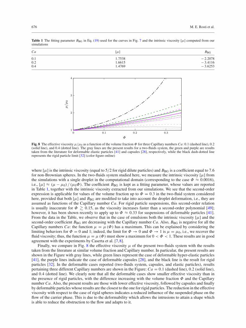
Table 1 The fitting parameter BBG in Eq. (19) used for the curves in Fig. 7 and the intrinsic viscosity [μ] computed from oursimulations

Ca [μ] BBG

0.1 1.7538 − 2.20780.2 1.6615 − 3.41160.4 1.4769 − 3.6253

1

2

3

4

0 0.1 0.2 0.3

μ/μ0

Φ

Fig. 8 The effective viscosity μ/μ0 as a function of the volume fractionΦ for three Capillary numbers Ca: 0.1 (dashed line), 0.2(solid line), and 0.4 (dotted line). The gray lines are the present results for a two-fluids system, the green and purple are resultstaken from the literature for deformable elastic particles [41] and capsules [28], respectively, while the black dash-dotted linerepresents the rigid particle limit [32] (color figure online)

where [μ] is the intrinsic viscosity (equal to 5/2 for rigid dilute particles) and BBG is a coefficient equal to 7.6for non-Brownian spheres. In the two-fluids system studied here, we measure the intrinsic viscosity [μ] fromthe simulations with a single droplet in the computational domain (corresponding to the case Φ ≈ 0.0016),i.e., [μ] ≈ (μ − μ0) / (μ0Φ). The coefficient BBG is kept as a fitting parameter, whose values are reportedin Table 1, together with the intrinsic viscosity extracted from our simulations. We see that the second-orderexpression is applicable for values of the volume fraction up to Φ = 0.3 in the two-fluid system consideredhere, provided that both [μ] and BBG are modified to take into account the droplet deformation, i.e., they areassumed as functions of the Capillary number Ca. For rigid particle suspensions, this second-order relationis usually inaccurate for Φ � 0.15, as the viscosity increases faster than a second-order polynomial [49];however, it has been shown recently to apply up to Φ ≈ 0.33 for suspensions of deformable particles [41].From the data in the Table, we observe that in the case of emulsions both the intrinsic viscosity [μ] and thesecond-order coefficient BBG are decreasing with the Capillary number Ca. Also, BBG is negative for all theCapillary numbers Ca: the function μ = μ (Φ) has a maximum. This can be explained by considering thelimiting behaviors for Φ = 0 and 1; indeed, the limit for Φ → 0 and Φ → 1 is μ = μ0, i.e., we recover thefluid viscosity; thus, the function μ = μ (Φ) must show a maximum for 0 < Φ < 1. These results are in goodagreement with the experiments by Caserta et al. [7,8].

Finally, we compare in Fig. 8 the effective viscosity μ of the present two-fluids system with the resultstaken from the literature at similar volume fraction and Capillary number. In particular, the present results areshown in the Figure with gray lines, while green lines represent the case of deformable hyper-elastic particles[41], the purple lines indicate the case of deformable capsules [28], and the black line is the result for rigidparticles [32]. In the deformable cases reported (two-fluids system, capsules, and elastic particles), resultspertaining three different Capillary numbers are shown in the Figure: Ca = 0.1 (dashed line), 0.2 (solid line),and 0.4 (dotted line). We clearly note that all the deformable cases show smaller effective viscosity than inthe presence of rigid particles, with the difference increasing with the volume fraction Φ and the Capillarynumber Ca. Also, the present results are those with lower effective viscosity, followed by capsules and finallyby deformable particles whose results are the closest to the one for rigid particles. The reduction in the effectiveviscosity with respect to the case of rigid spheres indicates a reduced influence of the suspended phase on theflow of the carrier phase. This is due to the deformability which allows the intrusions to attain a shape whichis able to reduce the obstruction to the flow and adapts to it.

Numerical simulations of emulsions in shear flows 677

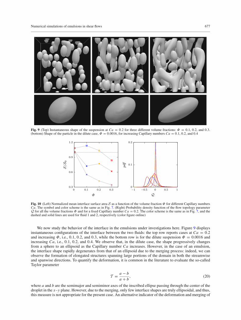
Fig. 9 (Top) Instantaneous shape of the suspension at Ca = 0.2 for three different volume fractions: Φ = 0.1, 0.2, and 0.3.(bottom) Shape of the particle in the dilute case, Φ = 0.0016, for increasing Capillary numbers Ca = 0.1, 0.2, and 0.4

0.3

0.6

0.9

1.2

0 0.1 0.2 0.3

S/S 0

Φ

0

0.1

0.2

−1 −0.5 0 0.5 1

pdf

Q

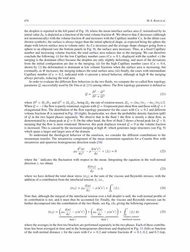
Fig. 10 (Left) Normalized mean interface surface area S as a function of the volume fraction Φ for different Capillary numbersCa. The symbol and color scheme is the same as in Fig. 7. (Right) Probability density function of the flow topology parameterQ for all the volume fractions Φ and for a fixed Capillary number Ca = 0.2. The color scheme is the same as in Fig. 7, and thedashed and solid lines are used for fluid 1 and 2, respectively (color figure online)

We now study the behavior of the interface in the emulsions under investigations here. Figure 9 displaysinstantaneous configurations of the interface between the two fluids: the top row reports cases at Ca = 0.2and increasing Φ, i.e., 0.1, 0.2, and 0.3, while the bottom row is for the dilute suspension Φ = 0.0016 andincreasing Ca, i.e., 0.1, 0.2, and 0.4. We observe that, in the dilute case, the shape progressively changesfrom a sphere to an ellipsoid as the Capillary number Ca increases. However, in the case of an emulsion,the interface shape rapidly degenerates from that of an ellipsoid due to the merging process: indeed, we canobserve the formation of elongated structures spanning large portions of the domain in both the streamwiseand spanwise directions. To quantify the deformation, it is common in the literature to evaluate the so-calledTaylor parameter

T = a − b

a + b, (20)

where a and b are the semimajor and semiminor axes of the inscribed ellipse passing through the center of thedroplet in the x–y plane. However, due to the merging, only few interface shapes are truly ellipsoidal, and thus,this measure is not appropriate for the present case. An alternative indicator of the deformation and merging of

678 M. E. Rosti et al.

the droplets is reported in the left panel of Fig. 10, where the mean interface surface area S, normalized by itsinitial value S0, is depicted as a function of the total volume fractionΦ. We observe that S decreases (althoughnot monotonically) with the volume fraction Φ and increases with the Capillary number Ca. In the dilute case(brown symbols), the surface is always larger than the initial spherical shape, as expected being the sphere theshape with lowest surface area to volume ratio. As Ca increases and the average shape changes going from asphere to an ellipsoid (see the bottom panels in Fig. 9), the surface area increases. Thus, at a fixed Capillarynumber and increasing volume fraction, the total surface area reduces due to the merging. We can thereforeconclude the following: (i) for the low Capillary number cases (Ca = 0.1, displayed with the symbol ×) themerging is the dominant effect because the droplets are only slightly deforming, and most of the deviationsfrom the initial configuration are due to the merging; (ii) for the high Capillary number cases (Ca = 0.4,shown by �) the deformation is dominant at low volume fractions when the surface area is increasing, buteventually, as Φ increases, the merging reduces the total surface area; (iii) finally, the cases with intermediateCapillary number (Ca = 0.2, indicated with ∗) present a mixed behavior, although at high Φ the mergingalways prevails, reducing the total area.

In order to evaluate the different flow behaviors in the two fluids, we compute the so-called flow topologyparameterQ, successfully used by De Vita et al. [11] among others. The flow topology parameter is defined as

Q = D2 − Ω2

D2 + Ω2 (21)

where D2 = Di j D ji and Ω2 = Ωi jΩ j i , being Ωi j the rate of rotation tensor, Ωi j = (∂ui/∂x j − ∂u j/∂xi )/2.WhenQ = −1 the flow is purely rotational, regionswithQ = 0 represent pure shear flow and thosewithQ = 1elongational flow. The distribution of the flow topology parameter for the cases with Ca = 0.2 and differentvolume fractions Φ is reported in Fig. 10 (right). In particular, we show the probability density function (pdf)of Q in the two liquid phases separately. We observe that in the fluid 1 the flow is mostly a shear flow, asdemonstrated by a sharp peak atQ = 0. On the other hand, the flow of fluid 2 shows a broad peak for Q < 0,meaning that the flow is more rotational. However, this peak displaces toward Q = 0 as the volume fractionis increased. This is caused by the increased merging at high Φ, which generates large structures (see Fig. 9)which spans a larger and larger area of the domain.

To understand the rheological behavior of the emulsion, we consider the different contributions to themomentum transfer. The streamwise component of the mean momentum equations for a Couette flow withstreamwise and spanwise homogeneous direction reads [34]

μ0d2〈u〉dy2

− ρd〈u′v′〉dy

+ 〈 f1〉 = 0 (22)

where the ′ indicates the fluctuation with respect to the mean. Integrating the equation in the wall-normaldirection y, we obtain

d〈σ12〉dy

= 0 (23)

where we have defined the total shear stress 〈σ12〉 as the sum of the viscous and Reynolds stresses, with theaddition of a contribution from the interfacial tension fi , i.e.,

〈σ12〉 = μ0d〈u〉dy

− ρ〈u′v′〉 +∫ y

0〈 f1〉. (24)

Note that, although the integral of the interfacial tension over a full droplet is null, the wall-normal profile ofits contribution is not, and it must thus be accounted for. Finally, the viscous and Reynolds stresses can befurther decomposed into the contribution of the two fluids, see Eq. (4), giving the following expression:

〈σ12〉 =(

μ0d〈u〉dy

− ρ〈u′v′〉)

︸ ︷︷ ︸fluid 1

+(

μ0d〈u〉dy

− ρ〈u′v′〉)

︸ ︷︷ ︸fluid 2

+∫ y

0〈 f1〉 dy︸ ︷︷ ︸

interfacial tension

(25)

where the averages in the first two brackets are performed separately in the two phases. Each of these contribu-tions has been averaged in time and in the homogeneous directions and displayed in Fig. 11 (left) as functionof the wall-normal distance y for the cases with Ca = 0.2 and volume fractions Φ = 0.1, 0.2, and 0.3 (top,

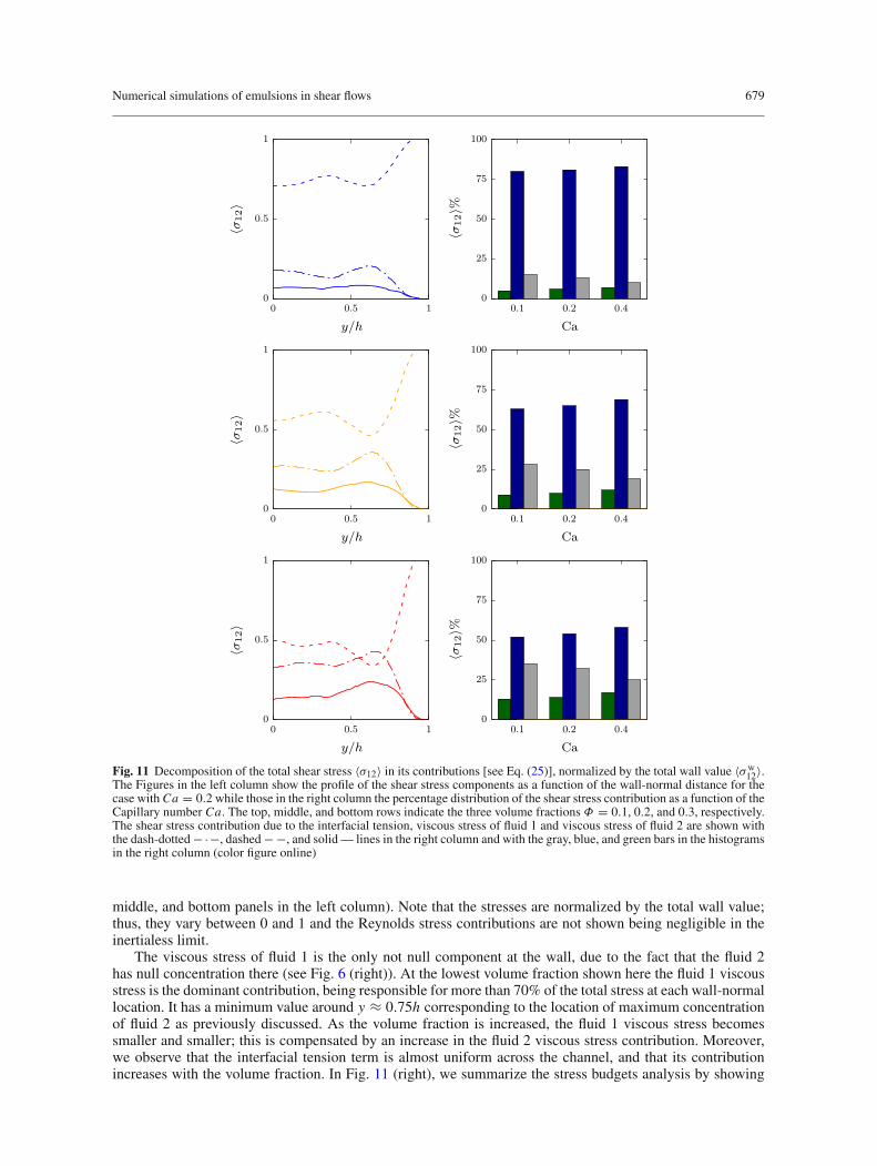
Numerical simulations of emulsions in shear flows 679

0

0.5

1

0 0.5 1

σ12

y/h

0

25

50

75

100

0.1 0.2 0.4

σ12%

Ca

0

0.5

1

0 0.5 1

σ12

y/h

0

25

50

75

100

0.1 0.2 0.4

σ12%

Ca

0

0.5

1

0 0.5 1

σ12

y/h

0

25

50

75

100

0.1 0.2 0.4

σ12%

Ca

Fig. 11 Decomposition of the total shear stress 〈σ12〉 in its contributions [see Eq. (25)], normalized by the total wall value 〈σw12〉.

The Figures in the left column show the profile of the shear stress components as a function of the wall-normal distance for thecase withCa = 0.2 while those in the right column the percentage distribution of the shear stress contribution as a function of theCapillary number Ca. The top, middle, and bottom rows indicate the three volume fractions Φ = 0.1, 0.2, and 0.3, respectively.The shear stress contribution due to the interfacial tension, viscous stress of fluid 1 and viscous stress of fluid 2 are shown withthe dash-dotted−·−, dashed− −, and solid— lines in the right column and with the gray, blue, and green bars in the histogramsin the right column (color figure online)

middle, and bottom panels in the left column). Note that the stresses are normalized by the total wall value;thus, they vary between 0 and 1 and the Reynolds stress contributions are not shown being negligible in theinertialess limit.

The viscous stress of fluid 1 is the only not null component at the wall, due to the fact that the fluid 2has null concentration there (see Fig. 6 (right)). At the lowest volume fraction shown here the fluid 1 viscousstress is the dominant contribution, being responsible for more than 70% of the total stress at each wall-normallocation. It has a minimum value around y ≈ 0.75h corresponding to the location of maximum concentrationof fluid 2 as previously discussed. As the volume fraction is increased, the fluid 1 viscous stress becomessmaller and smaller; this is compensated by an increase in the fluid 2 viscous stress contribution. Moreover,we observe that the interfacial tension term is almost uniform across the channel, and that its contributionincreases with the volume fraction. In Fig. 11 (right), we summarize the stress budgets analysis by showing

680 M. E. Rosti et al.

the volume-averaged percentage contribution of all the nonzero components of the total shear stress, i.e., fluid1 viscous stress (blue), fluid 2 viscous stress (green), and interfacial tension (gray). Each panel shows how thestress balance changes with the Capillary number, and each panel corresponds to a different volume fraction(Φ = 0.1: top panel; 0.2: middle panel; 0.3: bottom panel). For every volume fraction, we observe that thepercentage contribution of the viscous stress of the solvent and suspended fluids increases with the Capillarynumber; on the other hand, the contribution of the interfacial tension slightly decreases with the Capillarynumber (see Fig. 10 (left)). These results are similar to the one reported for hyper-elastic particles by Rostiand Brandt [41] who also found an increase in the particle contribution with the elasticity Capillary number(i.e., deformability).

4 Conclusions

We have implemented and validated a volume of fluid methodology based on the MTHINC method firstproposed by Ii et al. [21]which can be used to studymultiphase problems.A fullymulti-dimensional hyperbolictangent function is used to reconstruct the interface, and the main advantages can be summarized as follows: (i)the geometric reconstruction of the interface is not required; (ii) both linear and quadratic surfaces can be easilyconstructed; (iii) the continuous multi-dimensional hyperbolic tangent function allows the direct calculationsof the numerical fluxes, derivatives, and normal vectors; (iv) the hyperbolic tangent function prevents thenumerical diffusion that smears out the interface transition layer. Moreover, the implementation presentedhere allows the use of an efficient FFT-based fractional-step method to solve the system of equations and isbased on the splitting of the pressure in a constant and a varying term, which makes the FFT solver applicablealso when the density in the two phases differs.

We have studied the rheology of a system of two Newtonian fluids in a wall-bounded shear flow, i.e., planeCouette flow, at low Reynolds number such that inertial effects are negligible. The rheology of the emulsionis analyzed by discussing how the effective viscosity μ is affected by variations of the volume fraction Φ andCapillary numberCa. The effective viscosityμ is a nonlinear function of both these parametersμ = μ (Φ,Ca),and the emulsion shows an effective viscosity lower than the one of suspensions of rigid particles, deformableelastic particles, and capsules. Differently from these other cases, here the droplets can merge, especially athigh volume fractions and high Capillary numbers. Also, the effective viscosity curve has a negative secondderivativewith respect toΦ, thus suggesting the presence of amaximum in the curve at higher volume fractions.The overall deformation of the emulsion has been quantified in terms of the interface surface area and the flowwithin the two phases studied by means of the flow topology parameter. In particular, we have shown that theflow of the suspending fluid is mainly a shear flow, while that of the dispersed fluid is more rotational.

Finally, we have analyzed the contributions to the total shear stress of the two fluid phases and of theinterfacial force and showed that the Reynolds stress contributions are negligible at this Reynolds numberand that the viscous stress of the two fluids provides the dominant contribution. These have a non-uniformdistribution across the channel, with the percentage contribution of both phases increasing with the volumefraction and Capillary number. An important contribution comes from the interfacial tension, whose effectincreases with the volume fraction and decreases with the Capillary number.

The study presented in this work will be extended to consider different viscosity and density ratios betweenthe two fluids, and to better understand the non-monotonic behavior of the effective viscosity and its effect onthe rheological behavior of emulsions.

Acknowledgements The work is supported by the Microflusa project. This effort receives funding from the European UnionHorizon 2020 research and innovation program under Grant Agreement no. 664823. L.B. and M.E.R. also acknowledge financialsupport by the European Research Council Grant no. ERC-2013-CoG-616186, TRITOS. The computer time was provided bySwedish National Infrastructure for Computing (SNIC).

Open Access This article is distributed under the terms of the Creative Commons Attribution 4.0 International License (http://creativecommons.org/licenses/by/4.0/), which permits unrestricted use, distribution, and reproduction in any medium, providedyou give appropriate credit to the original author(s) and the source, provide a link to the Creative Commons license, and indicateif changes were made.

References

1. Alizad Banaei, A., Loiseau, J.C., Lashgari, I., Brandt, L.: Numerical simulations of elastic capsules with nucleus in shearflow. Eur. J. Comput. Mech. 26, 1–23 (2017)

Numerical simulations of emulsions in shear flows 681

2. Aulisa, E., Manservisi, S., Scardovelli, R., Zaleski, S.: A geometrical area-preserving volume-of-fluid advection method. J.Comput. Phys. 192(1), 355–364 (2003)

3. Batchelor, G.K.: The effect of Brownian motion on the bulk stress in a suspension of spherical particles. J. Fluid Mech.83(01), 97–117 (1977)

4. Batchelor, G.K., Green, J.T.: The determination of the bulk stress in a suspension of spherical particles to order c2. J. FluidMech. 56(03), 401–427 (1972)

5. Brackbill, J.U., Kothe, D.B., Zemach, C.: A continuum method for modeling surface tension. J. Comput. Phys. 100(2),335–354 (1992)

6. Caserta, S., Guido, S.: Vorticity banding in biphasic polymer blends. Langmuir 28(47), 16254–16262 (2012)7. Caserta, S., Simeone, M., Guido, S.: A parameter investigation of shear-induced coalescence in semidilute PIB–PDMS

polymer blends: effects of shear rate, shear stress volume fraction, and viscosity. Rheol. Acta 45(4), 505–512 (2006)8. Caserta, S., Simeone, M., Guido, S.: Shear banding in biphasic liquid–liquid systems. Phys. Rev. Lett. 100(13), 137801

(2008)9. Cristini, V., Guido, S., Alfani, A., Blawzdziewicz, J., Loewenberg, M.: Drop breakup and fragment size distribution in shear

flow. J. Rheol. 47(5), 1283–1298 (2003)10. Cummins, S.J., Francois, M.M., Kothe, D.B.: Estimating curvature from volume fractions. Comput. Fluids 83(6–7), 425–434

(2005)11. De Vita, F., Rosti, M.E., Izbassarov, D., Duffo, L., Tammisola, O., Hormozi, S., Brandt, L.: Elastoviscoplastic flow in porous

media. J. Non-Newton. Fluid Mech. 258, 10–21 (2018)12. Dodd, M.S., Ferrante, A.: A fast pressure-correction method for incompressible two-fluid flows. J. Comput. Phys. 273,

416–434 (2014)13. Dodd, M.S., Ferrante, A.: On the interaction of Taylor length scale size droplets and isotropic turbulence. J. Fluid Mech.

806, 356–412 (2016)14. Dong, S., Shen, J.: A time-stepping scheme involving constant coefficient matrices for phase-field simulations of two-phase

incompressible flows with large density ratios. J. Comput. Phys. 231(17), 5788–5804 (2012)15. Einstein, A.: Investigations on the Theory of the Brownian Movement. Dover Publications, Mineola (1956)16. Ferrini, F., Ercolani, D., De Cindio, B., Nicodemo, L., Nicolais, L., Ranaudo, S.: Shear viscosity of settling suspensions.

Rheol. Acta 18(2), 289–296 (1979)17. Francois, M.M., Cummins, S.J., Dendy, E.D., Kothe, D.B., Sicilian, J.M., Williams, M.W.: A balanced-force algorithm for

continuous and sharp interfacial surface tension models within a volume tracking framework. J. Comput. Phys. 213(1),141–173 (2006)

18. Freund, J.B.: Numerical simulation of flowing blood cells. Ann. Rev. Fluid Mech. 46, 67–95 (2014)19. Harvie, D.J.E., Fletcher, D.F.: A new volume of fluid advection algorithm: the stream scheme. J. Comput. Phys. 162(1), 1–32

(2000)20. Hysing, S.R., Turek, S., Kuzmin,D., Parolini, N., Burman, E., Ganesan, S., Tobiska, L.: Quantitative benchmark computations

of two-dimensional bubble dynamics. Int. J. Numer. Methods Fluids 60(11), 1259–1288 (2009)21. Ii, S., Sugiyama, K., Takeuchi, S., Takagi, S., Matsumoto, Y., Xiao, F.: An interface capturing method with a continuous

function: the THINC method with multi-dimensional reconstruction. J. Comput. Phys. 231(5), 2328–2358 (2012)22. Kim, J., Moin, P.: Application of a fractional-step method to incompressible Navier–Stokes equations. J. Comput. Phys.

59(2), 308–323 (1985)23. Kulkarni, P.M., Morris, J.F.: Suspension properties at finite Reynolds number from simulated shear flow. Phys. Fluids

(1994-present) 20(4), 040602 (2008)24. Legendre, D., Daniel, C., Guiraud, P.: Experimental study of a drop bouncing on awall in a liquid. Phys. Fluids (1994-present)

17(9), 097105 (2005)25. Loewenberg, M.: Numerical simulation of concentrated emulsion flows. J. Fluids Eng. 120(4), 824–832 (1998)26. Loewenberg, M., Hinch, E.J.: Numerical simulation of a concentrated emulsion in shear flow. J. Fluid Mech. 321, 395–419

(1996)27. Mason, T.G.: New fundamental concepts in emulsion rheology. Curr. Opin. Colloid Interface Sci. 4(3), 231–238 (1999)28. Matsunaga, D., Imai, Y., Yamaguchi, T., Ishikawa, T.: Rheology of a dense suspension of spherical capsules under simple

shear flow. J. Fluid Mech. 786, 110–127 (2016)29. Mewis, J., Wagner, N.J.: Colloidal Suspension Rheology. Cambridge University Press, Cambridge (2012)30. Noh, W.F., Woodward, P.: SLIC (simple line interface calculation). In: Proceedings of the Fifth International Conference on

Numerical Methods in Fluid Dynamics, pp. 330–340. Springer (1976)31. Picano, F., Breugem, W.P., Mitra, D., Brandt, L.: Shear thickening in non-Brownian suspensions: an excluded volume effect.

Phys. Rev. Lett. 111(9), 098302 (2013)32. Picano, F., Breugem, W.P., Brandt, L.: Turbulent channel flow of dense suspensions of neutrally buoyant spheres. J. Fluid

Mech. 764, 463–487 (2015)33. Pilliod Jr., J.E., Puckett, E.G.: Second-order accurate volume-of-fluid algorithms for tracking material interfaces. J. Comput.

Phys. 199(2), 465–502 (2004)34. Pope, S.B.: Turbulent Flows. Cambridge University Press, Cambridge (2001)35. Popinet, S., Zaleski, S.: A front-tracking algorithm for accurate representation of surface tension. Int. J. Numer. Methods

Fluids 30(6), 775–793 (1999)36. Prosperetti, A., Tryggvason, G.: Computational Methods for Multiphase Flow. Cambridge University Press, Cambridge

(2009)37. Puckett, E.G., Almgren, A.S., Bell, J.B., Marcus, D.L., Rider, W.J.: A high-order projection method for tracking fluid

interfaces in variable density incompressible flows. J. Comput. Phys. 130(2), 269–282 (1997)38. Quintard, M., Whitaker, S.: Transport in ordered and disordered porous media II: generalized volume averaging. Transp.

Porous Media 14(2), 179–206 (1994)39. Rider, W.J., Kothe, D.B.: Reconstructing volume tracking. J. Comput. Phys. 141(2), 112–152 (1998)

682 M. E. Rosti et al.

40. Rosti, M.E., Brandt, L.: Numerical simulation of turbulent channel flow over a viscous hyper-elastic wall. J. Fluid Mech.830, 708–735 (2017)

41. Rosti, M.E., Brandt, L.: Suspensions of deformable particles in a Couette flow. J. Non-Newton. Fluid Mech. https://doi.org/10.1016/j.jnnfm.2018.01.008 (2018) (accepted)

42. Rosti, M.E., Brandt, L., Mitra, D.: Rheology of suspensions of viscoelastic spheres: deformability as an effective volumefraction. Phys. Rev. Fluids 3(1), 012301(R) (2018)

43. Rudman, M.: Volume-tracking methods for interfacial flow calculations. Int. J. Numer. Methods Fluids 24(7), 671–691(1997)

44. Sacanna, S., Pine, D.J.: Shape-anisotropic colloids: building blocks for complex assemblies. Curr. Opin. Colloid InterfaceSci. 16(2), 96–105 (2011)

45. Scardovelli, R., Zaleski, S.: Direct numerical simulation of free-surface and interfacial flow. Ann. Rev. Fluid Mech. 31(1),567–603 (1999)

46. Sethian, J.A.: Level Set Methods and Fast Marching Methods: Evolving Interfaces in Computational Geometry, FluidMechanics, Computer Vision, and Materials Science, vol. 3. Cambridge University Press, Cambridge (1999)

47. Sethian, J.A., Smereka, P.: Level set methods for fluid interfaces. Ann. Rev. Fluid Mech. 35(1), 341–372 (2003)48. Singh, A., Nott, P.R.: Experimental measurements of the normal stresses in sheared Stokesian suspensions. J. Fluid Mech.

490, 293–320 (2003)49. Stickel, J.J., Powell, R.L.: Fluid mechanics and rheology of dense suspensions. Ann. Rev. Fluid Mech. 37, 129–149 (2005)50. Sussman, M., Smereka, P., Osher, S.: A level set approach for computing solutions to incompressible two-phase flow. J.

Comput. Phys. 114(1), 146–159 (1994)51. Takeishi, N., Imai, Y., Ishida, S., Omori, T., Kamm, R.D., Ishikawa, T.: Cell adhesion during bullet motion in capillaries.

Am. J. Physiol. Heart Circ. Physiol. 311(2), H395–H403 (2016)52. Takeuchi, S., Yuki, Y., Ueyama, A., Kajishima, T.: A conservative momentum-exchange algorithm for interaction problem

between fluid and deformable particles. Int. J. Numer. Methods Fluids 64(10–12), 1084–1101 (2010)53. Torres, D.J., Brackbill, J.U.: The point-set method: front-tracking without connectivity. J. Comput. Phys. 165(2), 620–644

(2000)54. Tryggvason, G., Bunner, B., Esmaeeli, A., Juric, D., Al-Rawahi, N., Tauber, W., Han, J., Nas, S., Jan, Y.J.: A front-tracking

method for the computations of multiphase flow. J. Comput. Phys. 169(2), 708–759 (2001)55. Tryggvason,G., Sussman,M.,Hussaini,M.Y.: Immersed boundarymethods for fluid interfaces.Comput.MethodsMultiphase

Flow 37, 239–261 (2007)56. Tryggvason, G., Scardovelli, R., Zaleski, S.: Direct Numerical Simulations of Gas–Liquid Multiphase Flows. Cambridge

University Press, Cambridge (2011)57. Unverdi, S.O., Tryggvason, G.: A front-tracking method for viscous, incompressible, multi-fluid flows. J. Comput. Phys.

100(1), 25–37 (1992)58. Xia, Y., Gates, B., Yin, Y., Lu, Y.: Monodispersed colloidal spheres: old materials with new applications. Adv. Mater. 12(10),

693–713 (2000)59. Xiao, F., Honma, Y., Kono, T.: A simple algebraic interface capturing scheme using hyperbolic tangent function. Int. J.

Numer. Methods Fluids 48(9), 1023–1040 (2005)60. Yokoi, K.: Efficient implementation of THINC scheme: a simple and practical smoothed VOF algorithm. J. Comput. Phys.

226(2), 1985–2002 (2007)61. Youngs, D.L.: Time-dependent multi-material flow with large fluid distortion. Numer. Methods Fluid Dyn. 24, 273–285

(1982)62. Youngs,D.L.: An interface trackingmethod for a 3DEulerian hydrodynamics code. Technical Report 44/92,AtomicWeapons

Research Establishment (1984)63. Zalesak, S.T.: Fully multidimensional flux-corrected transport. J. Comput. Phys. 31, 335–362 (1979)64. Zarraga, I.E., Hill, D.A., Leighton Jr., D.T.: The characterization of the total stress of concentrated suspensions of noncolloidal

spheres in Newtonian fluids. J. Rheol. 44(2), 185–220 (2000)

Publisher’s Note Springer Nature remains neutral with regard to jurisdictional claims in published maps and institutionalaffiliations.