Embed Size (px)
Citation preview
J. Appl. Environ. Biol. Sci., 5(9S)64-74, 2015
© 2015, TextRoad Publication
ISSN: 2090-4274 Journal of Applied Environmental
and Biological Sciences
www.textroad.com
Corresponding author: A. Sadeghian - Department of Mathematics, Islamic Azad University of Yazd, Yazd, Iran. [email protected]
Numerical Solution of Fractional Telegraph Equation Using the Second Kind
Chebyshev Wavelets Method
A. Sadeghian* 1 , M. H. Heydari2
, M. R. Hooshmandasl3
and S. M. Karbassi4
1,4
Department of Mathematics, Islamic Azad University of Yazd, Yazd, Iran 2,3,4
Faculty of Mathematics, Yazd University, Yazd, Iran Received: March 26, 2014
Accepted: May 17, 2015
ABSTRACT
In this paper, the two-dimensional second kind Chebyshev wavelets are applied for numerical solution of the time-fractional
telegraph equation with Dirichlet boundary conditions. In this way, a new operational matrix of fractional derivative for the
second wavelets is derived and then this operational matrix has been employed to obtain the numerical solution of the above
mentioned problem. The main characteristic behind this approach is that it reduces such problems to those of solving a system
of algebraic equations which greatly simplifying the problem. The power of this manageable method is illustrated.
KEYWORDS:Second kind Chebyshev wavelet, Telegraph equation, Dirichlet boundary condition, Fractional derivative.
1. INTRODUCTION
In recent years, fractional calculus and differential equations have found enormous applications in mathematics, physics,
chemistry and engineering because of this fact that, a realistic modeling of a physical phenomenon having dependence not only
at the time instant, but also the previous time history can be successfully achieved by using fractional calculus. The application
of the fractional calculus have been demonstrated by many authors. For examples, it is applied to model the nonlinear
oscillation of earthquakes [1], fluid-dynamic traffic [2], frequency dependent damping behavior of many viscoelastic materials
[3], continuum and statistical mechanics [4], colored noise [5], solid mechanics [6], economics [7], signal processing [8], and
control theory [9]. However, during the last decade fractional calculus has attracted much more attention of physicist and
mathematicians. Due to the increasing applications, some schemes have been proposed to solve fractional differential
equations. The most frequently used methods are Adomian decomposition method (ADM) [10-12], homotopy perturbation
method [13], homotopy analysis method [14], Variational iteration method (VIM) [15, 16], Fractional differential transform
Method (FDTM) [17-22], Fractional difference method (FDM) [23], power series method [24], generalized block pulse
operational matrix method [25] and Laplace transform method [26]. Also, recently the operational matrices of fractional order
integration for the Haar wavelet [27], Legendre wavelet [28] and the Chebyshev wavelets of first kind [29, 30] and second kind
[31] have been developed to solve the fractional differential equations.
In this paper consider the time-fractional telegraph equation of order 2)<(1 ≤αα as:
[0,1].[0,1]),(),,(),(=),(),(),(2
2
1
1
×∈+∂
∂+
∂
∂+
∂
∂
−
−
txtxftxux
txutxut
txut α
α
α
α
(1)
where β
β
t∂
∂ denotes the Caputo fractional derivative of order β , that will be described in the next section. This equation is
commonly used in the study of wave propagation of electric signals in a cable transmission line and also in wave phenomena.
This equation has been also used in modeling the reaction-diffusion processes in various branches of engineering sciences and
biological sciences by many researchers (see [32] and references therein).
The main purpose of this paper is to apply the second kind Chebyshev wavelets for solving time-fractional telegraph
equation (1). In this way, we first describe some properties of the second kind Chebyshev polynomials and Chebyshev
wavelets. Then, a new operational matrix of fractional derivative for the second kind Chebyshev wavelets are derived and are
applied to obtain approximate solution for the under study problem. This paper is organized as follows: In Section 2, some
necessary definitions of the fractional calculus are reviewed. In Section 3, the second kind Chebyshev polynomials and the
second kind Chebyshev wavelets with some useful theorems are investigated. In Section 4, the proposed method is described.
In Section 5, some numerical examples are presented. Finally a conclusion is drawn in Section 6.
64
Sadeghian et al.,2015
2. Basic definitions In the development of theories of fractional derivatives and integrals, many definitions for fractional derivatives and integrals
are appeared, such as Riemann-Liouville and Caputo [33], which are described below:
Definition 2-1
A real function 0> ),( xxu , is said to be in the space R∈µµ
,C if there exists a real number )(> µp such that
)(=)(1xuxxu
p, where ][0,)(
1∞∈Cxu and it is said to be in the space
n
Cµ
if N∈∈ nCun
,
)(
µ.
Definition 2-2
The Riemann-Liouville fractional integration operator of order 0≥α of a function 1 , −≥∈ µµ
Cu , is defined as [33]:
( )
−
Γ−
∫0.=),(
0,>,)()()(
1
=)(1
0
α
α
α
α
α
xu
dttutxxuI
x
(2)
It has the following properties:
( ) ( ) ,1)(
1)(=),(=)( ϑαϑαβαβα
ϑα
ϑ++
++Γ
+ΓxxIxuIxuII (3)
where 0, ≥βα and 1> −ϑ .
Definition 2-3
The fractional derivative operator of order 0>α in the Caputo sense is defined as [33]:
( )
−−−Γ
∈
−−
∗
∫ .<<1,)()()(
1
,=,)(
=)()(1
0nndttutx
n
ndx
xud
xuDnn
x
n
n
α
α
α
α
α
N
(4)
where n is an integer, 0>x , and n
Cu1
∈ .
The useful relation between the Riemann-Liouvill operator and Caputo operator is given by the following expression:
( ) ,<10,>,!
)(0)(=)()(
1
0=
nnxj
xuxuxuDI
j
jn
j
≤−−+
−
∗ ∑ ααα
(5)
where n is an integer, 0>x , and n
Cu1
∈ .
For more details about fractional calculus see [33].
3. The second kind Chebyshev polynomials and wavelets
The well-known second kind Chebyshev polynomial )(zUm
form a complete set of orthogonal functions with respect to the
weight function 21=)( zzw − on the interval 1,1][− . They can be determined with the aid of the following recurrence
formula [34]:
,2,3,=),()(2=)(21
KnzUzzUzUmmm −−
−
with 1=)(0zU and zzU 2=)(
1. For practical use of these polynomials on the interval of interest [0,1] , it is necessary to
shift the defining domain by means of the following substitution:
1.01,2= ≤≤− xxz
So, the shifted second kind Chebyshev polynomials )(xUm
∗
are obtained on the interval [0,1] as 1)(2=)( −
∗
xUxUmm
. The orthogonality condition for these shifted polynomials is:
,4
=1)(21)()(2
1
0mnnm
dxxxUxU δπ
−−
∗∗
∫ (6)
where mn
δ is the Kroneker delta.
The analytic form of the shifted second kind Chebyshev polynomial is:
65
J. Appl. Environ. Biol. Sci., 5(9S)64-74, 2015
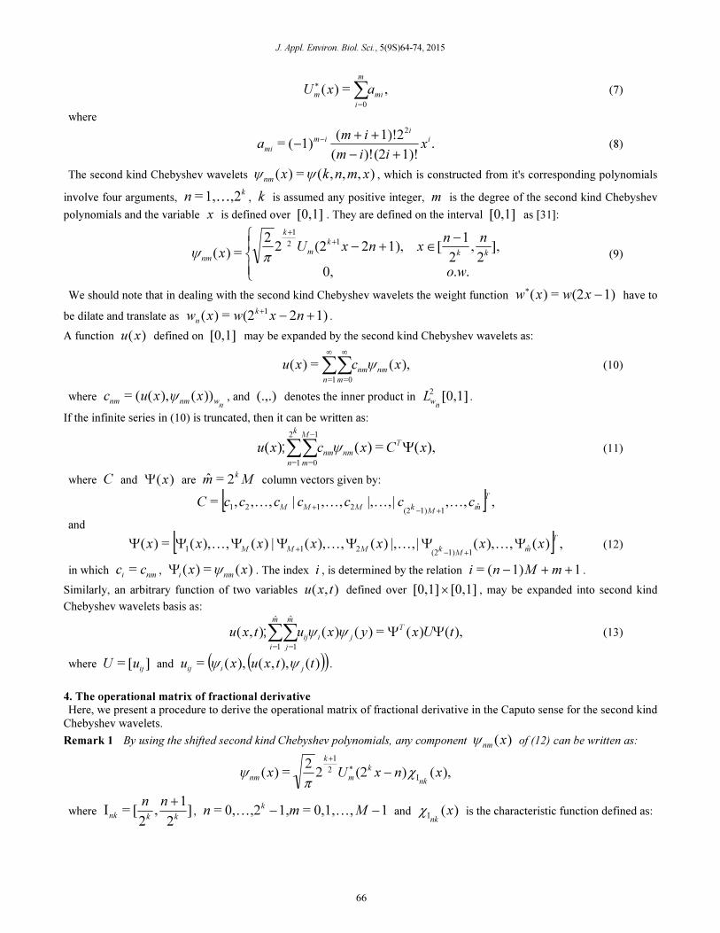
,=)(0=
mi
m
i
maxU ∑
∗
(7)
where
.1)!(2)!(
1)!2(1)(=
2
i
i
im
mix
iim
ima
+−
++−
−
(8)
The second kind Chebyshev wavelets ),,,(=)( xmnkxnm
ψψ , which is constructed from it's corresponding polynomials
involve four arguments, k
n ,21,= K , k is assumed any positive integer, m is the degree of the second kind Chebyshev
polynomials and the variable x is defined over [0,1] . They are defined on the interval [0,1] as [31]:
−∈+−+
+
..0,
],2,
2
1[1),2(22
2=)(
12
1
wo
nnxnxU
x kk
k
m
k
nm πψ (9)
We should note that in dealing with the second kind Chebyshev wavelets the weight function 1)(2=)( −
∗
xwxw have to
be dilate and translate as 1)2(2=)( 1+−
+
nxwxwk
n.
A function )(xu defined on [0,1] may be expanded by the second kind Chebyshev wavelets as:
),(=)(0=1=
xcxunmnm
mn
ψ∑∑∞∞
(10)
where n
wnmnmxxuc ))(),((= ψ , and (.,.) denotes the inner product in [0,1]
2
nw
L .
If the infinite series in (10) is truncated, then it can be written as:
),(=)()(1
0=
2
1=
xCxcxuT
nmnm
M
m
k
n
Ψ∑∑−
ψ; (11)
where C and )(xΨ are Mmk
2=ˆ column vectors given by:
[ ] ,,,|,|,,,|,,,= ˆ11)(22121
T
mM
kMMMcccccccC KKKK
+−+
and
[ ] ,)(,),(|,|,)(,),(|)(,),(=)( ˆ11)(2211
T
mM
kMMMxxxxxxx ΨΨΨΨΨΨΨ
+−+
KKKK (12)
in which nmicc = , )(=)( xx
nmiψΨ . The index i , is determined by the relation 11)(= ++− mMni .
Similarly, an arbitrary function of two variables ),( txu defined over [0,1][0,1]× , may be expanded into second kind
Chebyshev wavelets basis as:
),()(=)()(),(ˆ
1=
ˆ
1=
tUxyxutxuT
jiij
m
j
m
i
ΨΨ∑∑ ψψ; (13)
where ][=ijuU and ( )( ))(),,(),(= ttxuxu
jiijψψ .
4. The operational matrix of fractional derivative
Here, we present a procedure to derive the operational matrix of fractional derivative in the Caputo sense for the second kind
Chebyshev wavelets.
Remark 1 By using the shifted second kind Chebyshev polynomials, any component )(xnm
ψ of (12) can be written as:
),()(222
=)(I
2
1
xnxUxnk
k
m
k
nmχ
πψ −
∗
+
where ]2
1,
2[=I
kknk
nn +
, 1,0,1,=1,,20,= −− Mmnk
KK and )(I
xnk
χ is the characteristic function defined as:
66
Sadeghian et al.,2015
+∈
..0,
],2
1,
2[1,
=)(I
wo
nn
x
x
kk
nk
χ
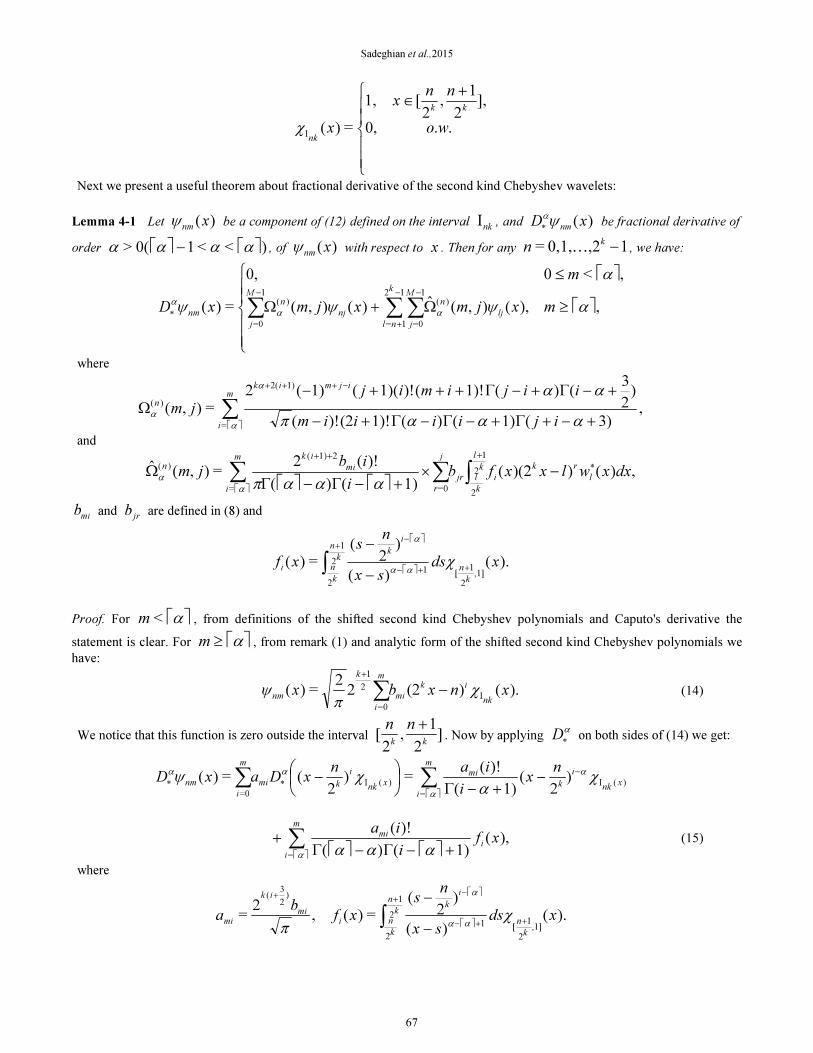
Next we present a useful theorem about fractional derivative of the second kind Chebyshev wavelets:
Lemma 4-1 Let )(xnm
ψ be a component of (12) defined on the interval nkI , and )(xD
nmψ
α
∗ be fractional derivative of
order )<<1(0> − αααα , of )(xnm
ψ with respect to x . Then for any 1,20,1,= −
kn K , we have:
≥Ω+Ω
≤
∑∑∑−−
+
−
∗,),(),(ˆ)(),(
,<00,
=)( )(1
0=
12
1=
)(1
0=
αψψ
α
ψαα
α
mxjmxjm
m
xD lj
nM
j
k
nl
nj
nM
j
nm
where
,3)(1)()(1)!(2)!(
)2
3()(1)!()!1)((1)(2
=),(
1)2(
=
)(
+−+Γ+−Γ−Γ+−
+−Γ+−Γ+++−
Ω
−+++
∑αααπ
ααα
α
α
ijiiiim
iijimij
jm
ijmikm
i
n
and
,)())(2(1)()(
)!(2=),(ˆ 2
1
20=
21)(
=
)( dxxwlxxfbi
ibjm l
rk
ik
l
k
ljr
j
r
mi
ikm
i
n ∗+++
−×+−Γ−Γ
Ω ∫∑∑αααπ
α
α
mib and
jrb are defined in (8) and
).()(
)2
(=)(
,1]2
1[1
2
1
2
xdssx
ns
xfk
n
i
kk
n
k
ni ++−
−+
−
−
∫ χαα
α
Proof. For α<m , from definitions of the shifted second kind Chebyshev polynomials and Caputo's derivative the
statement is clear. For ≥ αm , from remark (1) and analytic form of the shifted second kind Chebyshev polynomials we
have:
).()(222
=)(I
0=
2
1
xnxbxnk
ik
mi
m
i
k
nmχ
πψ −∑
+
(14)
We notice that this function is zero outside the interval ]2
1,
2[
kk
nn +
. Now by applying α
∗D on both sides of (14) we get:
)(I
=
)(I
0=
)2
(1)(
)!(=)
2(=)(
xnk
i
k
mi
m
i
xnk
i
kmi
m
i
nm
nx
i
ianxDaxD χ
αχψ
α
α
αα −
∗∗ −
+−Γ
− ∑∑
),(1)()(
)!(
=
xfi
iai
mi
m
i +−Γ−Γ+ ∑
αααα
(15)
where
).()(
)2
(=)(,
2=
,1]2
1[1
2
1
2
)2
3(
xdssx
ns
xfb
ak
n
i
kk
n
k
ni
mi
ik
mi ++−
−++
−
−
∫ χπ
αα
α
67
J. Appl. Environ. Biol. Sci., 5(9S)64-74, 2015
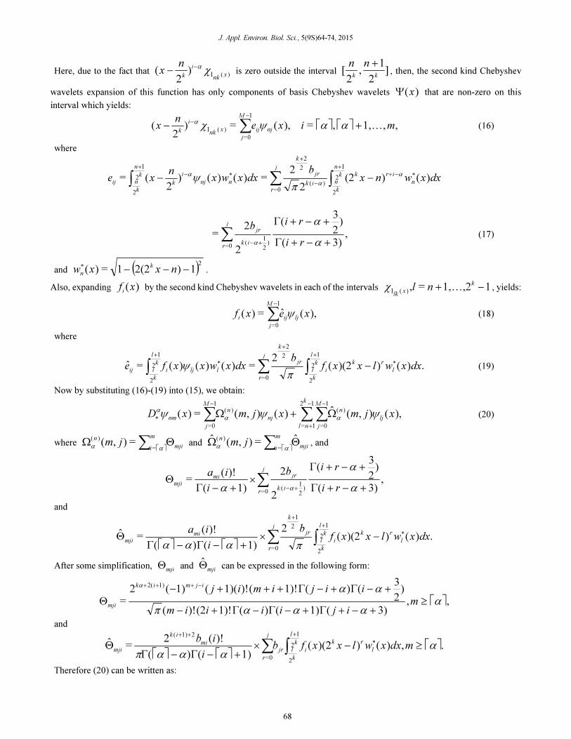
Here, due to the fact that )(I)2
(x
nk
i
k
n
x χα−
− is zero outside the interval ]2
1,
2[
kk
nn +
, then, the second kind Chebyshev
wavelets expansion of this function has only components of basis Chebyshev wavelets )(xΨ that are non-zero on this
interval which yields:
,,1,,=),(=)2
(1
0=
)(I mixen
x njij
M
j
xnk
i
kK+− ∑
−
−
ααψχα
(16)
where
dxxwnxb
dxxwxn
xe n
irkk
n
k
nik
jr
k
j
r
nnj
i
k
k
n
k
nij )()(22
2=)()()
2(= 2
1
2
)(
2
2
0=
2
1
2
∗−+
+
−
+
∗−
+
−− ∫∑∫α
α
α
πψ
,3)(
)2
3(
2
2=
)2
1(
0= +−+Γ
+−+Γ
+−
∑α
α
α ri
rib
ik
jrj
r
(17)
and ( )21)2(21=)( −−−
∗
nxxwk
n.
Also, expanding )(xfi
by the second kind Chebyshev wavelets in each of the intervals 1,21,=,)(I −+k
xlk
nl Kχ , yields:
),(ˆ=)(1
0=
xexf ljij
M
j
i ψ∑−
(18)
where
.)())(2(2
=)()()(=ˆ 2
1
2
2
2
0=
2
1
2
dxxwlxxfb
dxxwxxfe l
rk
ik
l
k
l
jr
k
j
r
lljik
l
k
lij
∗
+
+
∗
+
−∫∑∫π
ψ (19)
Now by substituting (16)-(19) into (15), we obtain:
),(),(ˆ)(),(=)( )(1
0=
12
1=
)(1
0=
xjmxjmxD lj
nM
j
k
nl
nj
nM
j
nm ψψψαα
α Ω+Ω ∑∑∑−−
+
−
∗ (20)
where mji
m
i
njm ΘΩ ∑ αα =
)(=),( and
mji
m
i
njm ΘΩ ∑
ˆ=),(ˆ=
)(
αα
, and
,3)(
)2
3(
2
2
1)(
)!(=
)2
1(
0= +−+Γ
+−+Γ
×+−Γ
Θ+−
∑α
α
α α ri
rib
i
ia
ik
jrj
r
mimji
and
.)())(2(2
1)()(
)!(=ˆ 2
1
2
2
1
0=
dxxwlxxfb
i
ial
rk
ik
l
k
l
jr
k
j
r
mimji
∗
+
+
−×+−Γ−Γ
Θ ∫∑πααα
After some simplification, mji
Θ and mji
Θ can be expressed in the following form:
,,3)(1)()(1)!(2)!(
)2
3()(1)!()!1)((1)(2
=
1)2(
≥+−+Γ+−Γ−Γ+−
+−Γ+−Γ+++−Θ
−+++
α
αααπ
ααα
mijiiiim
iijimijijmik
mji
and
.,)())(2(1)()(
)!(2=ˆ 2
1
20=
21)(
≥−×+−Γ−Γ
Θ ∗
+++
∫∑ ααααπ
mdxxwlxxfbi
ibl
rk
ik
l
k
ljr
j
r
mi
ik
mji
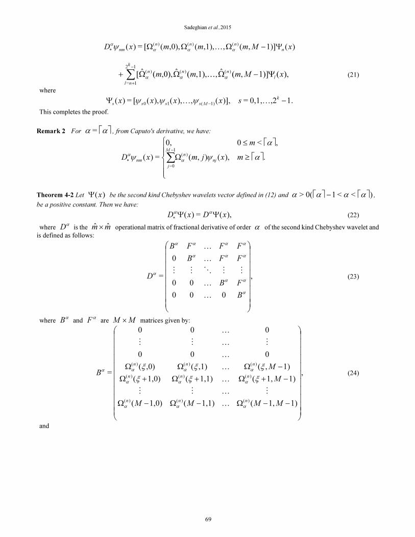
Therefore (20) can be written as:
68
Sadeghian et al.,2015
)(1)],(,,1),(,0),([=)( )()()(xMmmmxD
n
nnn
nmΨ−ΩΩΩ
∗ ααα
α
ψ K
),(1)],(ˆ,,1),(ˆ,0),(ˆ[)()()(
12
1=
xMmmml
nnn
k
nl
Ψ−ΩΩΩ+ ∑−
+
αααK (21)
where
1.,20,1,=)],(,),(),([=)( 1)(10 −Ψ−
k
Msssssxxxx KK ψψψ
This completes the proof.
Remark 2 For αα = , from Caputo's derivative, we have:
≥Ω
≤
∑−
∗.),(),(
,<00,
=)()(
1
0=
αψ
α
ψα
α
mxjm
m
xD nj
nM
j
nm
Theorem 4-2 Let )(xΨ be the second kind Chebyshev wavelets vector defined in (12) and )<<1(0> − αααα ,
be a positive constant. Then we have:
),(=)( xDxD ΨΨ∗
αα
(22)
where αD is the mm ˆˆ × operational matrix of fractional derivative of order α of the second kind Chebyshev wavelet and
is defined as follows:
,
000
00
0
=
α
αα
ααα
αααα
α
B
FB
FFB
FFFB
D
K
K
MMOMM
K
K
(23)
where α
B and αF are MM × matrices given by:
,
1)1,(1,1)(1,0)(
1)1,(1,1)(1,0)(
1),(,1)(,0)(
000
000
=
)()()(
)()()(
)()()(
−−Ω−Ω−Ω
−+Ω+Ω+Ω
−ΩΩΩ
MMMM
M
MB
nnn
nnn
nnn
ααα
ααα
αααα
ξξξ
ξξξ
K
MKMM
K
K
K
MKMM
K
(24)
and
69
J. Appl. Environ. Biol. Sci., 5(9S)64-74, 2015
,
1)1,(ˆ1,1)(ˆ1,0)(ˆ
1)1,(ˆ1,1)(ˆ1,0)(ˆ
1),(ˆ,1)(ˆ,0)(ˆ
000
000
=
)()()(
)()()(
)()()(
−−Ω−Ω−Ω
−+Ω+Ω+Ω
−ΩΩΩ
MMMM
M
MF
nnn
nnn
nnn
ααα
ααα
αααα
ξξξ
ξξξ
K
MKMM
K
K
K
MKMM
K
(25)
and αξ = .
Proof. It is an immediate consequence of the lemma 4.1.
Remark 3 From remark 2, it must be noted that for αα = , we have 0=α
F .
5. Description of the proposed method In this section, we apply the operational matrix of fractional derivative for second kind Chebyshev wavelet for solving
fractional telegraph equation (1) with the boundary conditions:
).(=)(1,),(=,1)(
),(=)(0,),(=,0)(
11
00
tgtuxfxu
tgtuxfxu (26)
For this purpose, we suppose:
),()(=),( tUxtxuT
ΨΨ (27)
where mmji
uU ˆˆ, ][=×
is an unknown matrix which should be found and (.)Ψ is the vector which is defined in (12). Now
using (13) and (22), we obtain:
),()(=),( tUDxtxut
TΨΨ
∂
∂α
α
α
(28)
),()(=),( 1
1
1
tUDxtxut
T ΨΨ∂
∂−
−
−
α
α
α
(29)
and
).())((=),(2
2
2
tUxDtxux
TΨΨ
∂
∂ (30)
Also using (13), the function ),( txf in (1) can be approximated as:
),()(),( tBxtxf TΨΨ; (31)
where ][=ij
BB is a mm ˆˆ × known matrix with entries ( )( ))(),,(),(= ttxfxBjiij
ψψ . Substituting (27)-(31) in (1)
consequent:
[ ] 0.=)()()()( 21tBUDUDDUx
TTΨ−−++Ψ
−αα
(32)
The entries of vectors )(xΨ and )(tΨ in (32) are independent, so we have:
0.=)()(= 21BUDUDDUH
T−−++
−αα
(33)
Here, we choose 22)ˆ( −m equations of (33) as:
1.ˆ,2,=,0,= −mjiHij
K (34)
We can also approximate the functions )(0 xf , )(1xf , )(
0tg and )(
1tg as:
70
Sadeghian et al.,2015
),(=)(),(=)(
),(=)(),(=)(
4121
3010
tCtgxCxf
tCtgxCxfTT
TT
ΨΨ
ΨΨ (35)
where 1
C , 2
C , 3C and 4
C are known vectors of dimension m .
Applying (27) and (35) in the boundary conditions (26), we have:
).(=)((1),)(=(1))(
),(=)((0),)(=(0))(
42
31
tCyUCxUx
tCyUCxUxTTTT
TTTT
ΨΨΨΨΨΨ
ΨΨΨΨΨΨ (36)
The entries of vectors )(xΨ and )(tΨ are independent, so from (36) we obtain:
0.=(1)=0,=(1)=
0,=(0)=0,=(0)=
4422
3311
TT
TT
CUCU
CUCU
−ΨΛ−ΨΛ
−ΨΛ−ΨΛ (37)
By choosing the m equations of 1,2)=( 0= jj
Λ and 2ˆ −m equations of 3,4)=( 0= jj
Λ , we get 4ˆ4 −m
equations, i.e.
1.ˆ,2,3,=3,4,=0,=
,ˆ,1,2,=1,2,=0,=
−Λ
Λ
mij
mij
ji
ji
K
K
(38)
Equetion (34) together (38) give 2
m equations, which can be solved for iju , mji ˆ,1,2=, K . So the unknown function
),( txu can be found.
6 . Numerical examples In this section, we demonstrate the efficiency of the proposed method for numerical solution of the telegraph equation in
the form of (1) with the boundary conditions (26).
Example 1 Consider the time-fractional telegraph equation (1) with 1=),( 2−+ txtxf and the boundary conditions
as:
.1=)(1,,1=,1)(
,=)(0,,=,0)(2
2
ttuxxu
ttuxxu
++
The exact solution of this problem for 2=α is txtxu +2=),( . Numerical solutions for some different values of α and
[0,1]∈t for 3)=1,=(6=ˆ Mkm are shown in Fig. 1. The values of exact solution ( 2=α ) and approximate solutions
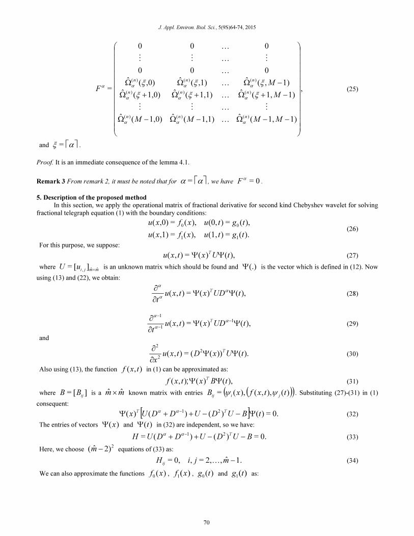
for some different values of α and some nodes ),( yx in [0,1][0,1]× , for 6=m are shown in Table 1.
Table1.Comparison between the exact ( 2=α ) and numerical solutions for Example ??.
),( ii yx 1.4=α 1.6=α 1.8=α Exact solution
(0.2,0.2) 0.26551095384623 0.25900735191924 0.25037754779349 0.24000000000000
(0.4,0.4) 0.61739964615400 0.60276654181831 0.58334948253535 0.56000000000000
(0.6,0.6) 1.01739964615401 1.00276654181831 0.98334948253536 0.96000000000000
(0.8,0.8) 1.46551095384624 1.45900735191925 1.45037754779350 1.44000000000000
(1.0,1.0 1.99999999999999 1.99999999999999 1.99999999999999 2.00000000000000
71

J. Appl. Environ. Biol. Sci., 5(9S)64-74, 2015
Fig.1.Numerical solutions of Example 1 for some different values of α .
Example 2 Consider time-fractional telegraph equation (1) with 0=),( txf and the boundary conditions as:
.=)(1,,=,1)(
,=)(0,,=,0)(11 tx
tx
etuexu
etuexu
−−
−
The exact solution of this problem for 2=α is tx
etxu−=),( . Numerical solutions for some different values of α and
[0,1]∈t for 4)=1,=(8=ˆ Mkm are shown in Fig. 2. The values of the exact solution ( 2=α ) and approximate
solutions for some different values of α and some nodes ),( yx in [0,1][0,1]× , for 8=m are shown in Table 2.
Table 2.Comparison between the exact ( 2=α ) and numerical solutions for Example 2.
),(iiyx
1.4=α
1.6=α
1.8=α
Exact solution
(0.2,0.2)
1.00325555517139 1.00391875185692 1.00627606867049 1.00000000000000
(0.4,0.4)
1.00541907760911 1.00685195815738 1.01150179716283 1.00000000000000
(0.6,0.6)
1.00546382142790 1.00673580015166 1.01056465711498 1.00000000000000
(0.8,0.8)
1.00334917683010 1.00379783774964 1.00506051184037 1.00000000000000
(1.0,1.0
0.99944928830814 0.99944928830812 0.99944928830815 1.00000000000000
72
Sadeghian et al.,2015
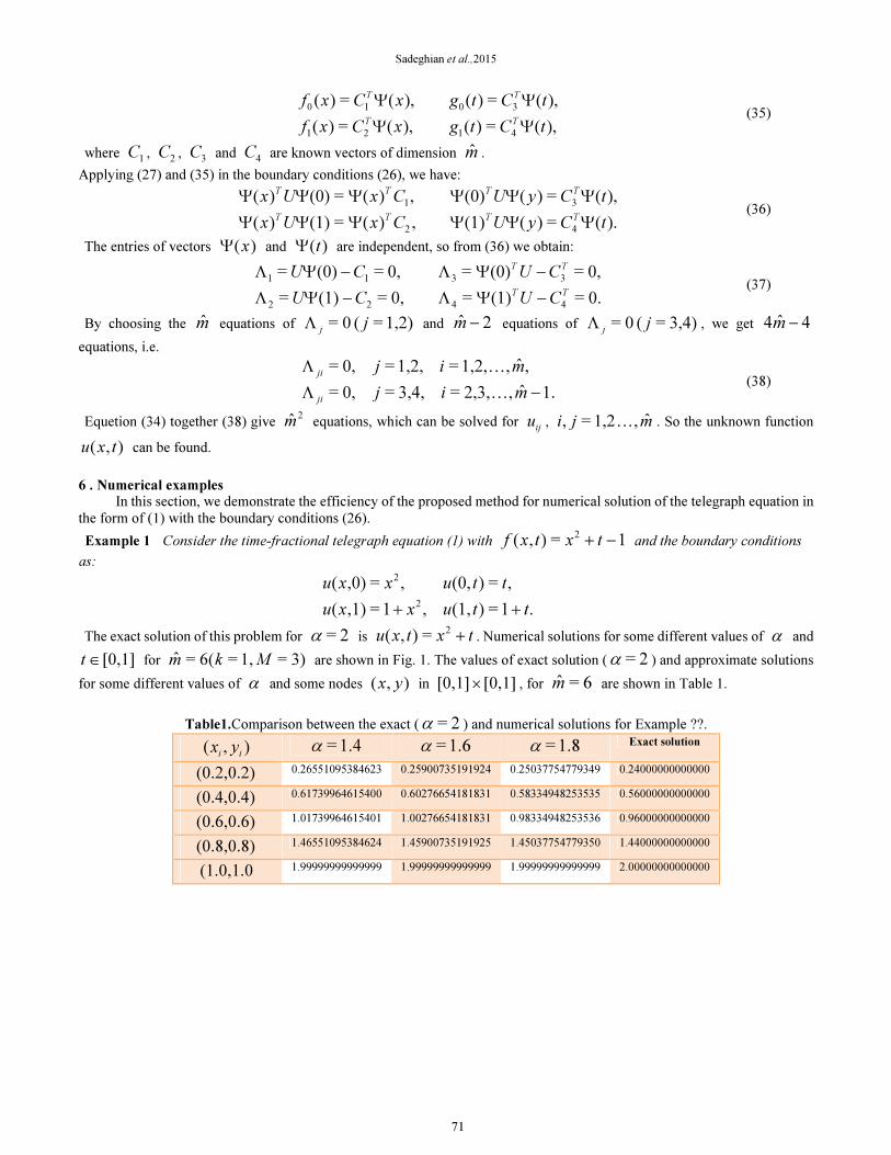
Fig.2.Numerical solutions of Example 2 for some different values of α .
Conclusion In this paper, a numerical method for approximating the solution of the time-fractional telegraph equation with Dirichlet
boundary condition by combining second kind Chebyshev wavelet function with their operational matrix of fractional
derivatives was presented. The method was shown that is very convenient for solving boundary value problems. Also, the
implementation of the proposed method is very simple and is very efficient for solution of the telegraph problem. Moreover, the
proposed method can be used for numerical solution of other kinds of fractional partial differential equations such as Poisson
and diffusion equations.
REFERENCES
1. J. H. He, Nonlinear oscillation with fractional derivative and its applications,’ International conference on vibrating
engineering98. China: Dalian, p. 288-291, 1998.
2. J. H. He, Some applications of nonlinear fractional differential equations and their approximations, 'Bull Sci Technol, vol.
15(2), p. 86-90, 1999.
3. R. L. Bagley and P. J. Torvik, A theoretical basis for the application of fractional calculus to viscoelasticity, J Rheol, 27(3), p.
201-210, 1983.
4. F. Mainardi, Fractional calculus: some basic problems in continuum and statistical mechanics, Carpinteri A, Mainardi F,
editors. Fractals and fractional calculus in continuum mechanics. New York: Springer, Verlag, p. 291-348, 1997.
5. B. Mandelbrot, Some noises with f1/
spectrum, a bridge between direct current and white noise, IEEE Trans Inform
Theory, 13(2), p. 289-98, 1967.
6. Y. A. Rossikhin and M. V. Shitikova, Applications of fractional calculus to dynamic problems of linear and nonlinear
hereditary mechanics of solids, Appl Mech Rev, 50, pp. 15--67, 1997.
7. R. T. Baillie, Long memory processes and fractional integration in econometrics, J Econometrics, 73, p. 55-59, 1996.
8. R. Panda and M. Dash, Fractional generalized splines and signal processing, Signal Process, vol. 86, pp. 2340--2350, 2006.
9. G. W. Bohannan, Analog fractional order controller in temperature and motor control applications, J. Vib. Control, 14, p.
1487-1498, 2008.
73

J. Appl. Environ. Biol. Sci., 5(9S)64-74, 2015
10. Z. Odibat and S. Momani, Numerical methods for nonlinear partial differential equations of fractional order, Appl. Math.
Model, 32, p. 28-39, 2008.
11. S. Momani and Z. Odibat, Numerical approach to differential equations of fractional order, J. Comput. Appl. Math, 207, p.
96-110, 2007.
12. S. A. El-Wakil, A. Elhanbaly, and M. Abdou, Adomian decomposition method for solving fractional nonlinear differential
equations, Appl. Math. Comput, 182, p. 313-324, 2006.
13. N. H. Sweilam, M. M. Khader, and R. F. Al-Bar, Numerical studies for a multi-order fractional differential equation,
Physics Letters A, 371, p. 26-33, 2007.
14. I. Hashim, O. Abdulaziz, and S. Momani, Homotopy analysis method for fractional ivps, Commun. Nonlinear Sci. Numer.
Simul, 14, p. 674-684, 2009.
15. N. Sweilam, M. Khader, and R. Al-Bar, Numerical studies for a multi-order fractional differential equation, Phys. Lett. A,
371, p. 26-33, 2007.
16. S. Das, `Analytical solution of a fractional diffusion equation by variational iteration method, Comput. Math. Appl, vol. 57,
pp. 483--487, 2009.
17. A. Arikoglu and I. Ozkol, Solution of fractional differential equations by using differential transform method, Chaos,
Solitons Fract, 34, p. 1473-1481, 2007.
18. A. Arikoglu and I. Ozkol, Solution of fractional integro-differential equations by using fractional differential transform
method, Chaos, Solitons Fract, 40, p. 521-529, 2009.
19. P. Darania and A. Ebadian, A method for the numerical solution of the integro-differential equations, Appl. Math. Comput,
188, p. 657-668, 2007.
20. V. Erturk and S. Momani, Solving systems of fractional differential equations using differential transform method, J.
Comput. Appl. Math, 215, p. 142-151, 2008.
21. V. Erturk and S. Momani, Solving systems of fractional differential equations using differential transform method, J.
Comput. Appl. Math, 215, p. 142-151, 2008.
22. V. S. Erturk, S. Momani, and Z. Odibat, Application of generalized differential transform method to multi-order fractional
differential equations, Comm. Nonlinear Sci. Numer. Simulat, 13, p. 1642-1654, 2008.
23. M. Meerschaert and C. Tadjeran, Finite difference approximations for two-sided space-fractional partial differential
equations, Appl. Numer. Math, 56, p. 80-90, 2006.
24. Z. Odibat and N. Shawagfeh, Generalized taylor's formula, Appl. Math. Comput, 186, p. 286-293, 2007.
25. Y. L. Li and N. Sun, Numerical solution of fractional differential equation using the generalized block puls operational
matrix, Comput. Math. Appl, 62(3), p. 1046-1054, 2011.
26. I. Podlubny, The laplace transform method for linear differential equations of fractional order,
eprint<arxiv:funct-an/9710005>, 1997.
27. Y. Li and W. Zhao, Haar wavelet operational matrix of fractional order integration and its applications in solving the
fractional order differential equations, Appl. Math. Comput, 216, p. 2276-2285, 2010.
28. M. Rehman and R. A. Kh, The legendre wavelet method for solving fractional differential equations, Communications in
Nonlinear Science and Numerical Simulation, 16(11), p. 4163-4173, 2011.
29. Y. Li, Solving a nonlinear fractional differential equation using chebyshev wavelets, Communications in Nonlinear Science
and Numerical Simulation, 15(9), p. 228-2292, 2009.
30. M. H. Heydari, M. R. Hooshmandasl, F. M. M. Ghaini, and F. Mohammadi, Wavelet collocation method for solving multi
order fractional differential equations, Journal of Applied mathematics, 2012, Article ID 542401, 19 pages
doi:10.1155/2012/542401.
30. Y. Wang and Q. Fan, The second kind chebyshev wavelet method for solving fractional differential equations, Applied
Mathematics and Computation, 218, p. 8592-8601, 2012.
31. M. Lakestani and B. N. Saray, Numerical solution of telegraph equation using interpolating scaling functions, Comput.
Math. Appl, 60, p. 1964-1972, 2010.
32. I. Podlubny, Fractional Differential Equations. San Diego: Academic Press, 1999.
33. C.Canuto, M. Hussaini, A. Quarteroni, and T.Zang, Spectral methods in fluid dynamics, 1988.
74