NUMERICAL SOLUTION OF PRICING OF EUROPEAN CALL OPTION … · IJRRAS 13 (3) December 2012 Sánchez & Olivares Numerical Solution of Pricing of Call Option 667 In the mathematical literature,

IJRRAS 13 (3) ● December 2012 www.arpapress.com/Volumes/Vol13Issue3/IJRRAS_13_3_02.pdf

666

NUMERICAL SOLUTION OF PRICING OF EUROPEAN CALL OPTION

WITH STOCHASTIC VOLATILITY

Freddy H. Marín Sánchez1 & Manuela Bastidas Olivares

2

EAFIT University, Medellín, Colombia

Email: [email protected]; [email protected]

2

ABSTRACT

We propose a transformation that allows to build an explicit finite difference scheme for option pricing in stochastic

volatility models. The scheme is second order in space and first order in time. We present conditions of positivity and

monotonicity of the scheme. To test conditional stability results in the sense of von Neumann performing a Fourier

analysis of the problem and follows the convergence of our scheme. We present some numerical experimental results

for European call option pricing.

Keywords: Option pricing, explicit finite difference scheme, positivity, monotonicity.

1. INTRODUCTION The central model of option pricing theory is the Black-Scholes model (1973), which shows that, without making

assumptions about the preferences of investors, one can obtain an expression of the value of options that not directly

dependent on the expected performance of the underlying stock or the option. This is achieved through dynamic

hedging argument in a free market perfect arbitrage.

The assumptions of the Black-Scholes model form an ideal scenario, in which the continuous trading is possible, in

perfect markets, in which the interest rate is constant risk free and the price of the underlying asset behaves like a

geometric Brownian motion. However, some empirical studies have shown that these considerations are unrealistic

and do not explain a significant impact on financial markets such as volatility changes.

In this direction, there are sophisticated models that incorporate more accurate volatility as a random variable that is

set up as a second factor of risk in financial markets because not only the returns of assets are at risk.

This class of models known as stochastic volatility models. The most representative work in this regard is the model of

Heston (1993). This model is based on a system of two coupled stochastic differential equations that represent the

dynamic behavior of the underlying asset and the other dynamics of volatility and which are correlated Brownian

motions. Following the description in Düring and Fournié (2012), in such systems can be represented as

1= dZSVdtSdS tttt (1)

2)()(= dZVbdtVadV ttt (2)

dttdZtdZ =)()( 21 (3)

where is the trend term of the asset and )( tVa and )( tVb are respectively the coefficients of the diffusion and

trend of the stochastic volatility and is the correlation factor.

Similar arguments set in Black-Scholes (1973), allow to find the partial differential equation

0=)()(2

1)(

2

1 22 rFrSFFVaFVbSFVVbVFSF svvvSVSSt (4)

Where r is the free risk interest rate.

Equation (4) has been solved for 0>,VS , Tt 0 subject to the boundary conditions depending on the specific

type of option.

In general, the model Heston when the coefficients are not constant, equation (4) must be solved numerically.

Moreover, for the case where the option is the American type, must be solve a free boundary problem with a restriction

for the early exercise constraint for the option price. Also for this problem has to resort to numerical approximations.

mailto:[email protected]

mailto:[email protected]

IJRRAS 13 (3) ● December 2012 Sánchez & Olivares ● Numerical Solution of Pricing of Call Option

667

In the mathematical literature, there are many articles about numerical methods for option pricing, especially

addressing the case of a single risk factor, also second-order finite difference methods and more recently, high order

finite difference schemes. Other approaches include finite element, finite volume and spectral methods. (See, for

example, Düring and Fournié (2012) and references therein).

Other finite difference approaches used are standard methods of low order (second order in space) for option pricing in

stochastic volatility models. In D.Y. Tangman, A. Gopaul, and M. Bhuruth (2008) is considered a higher order

compact scheme (HOC) for parabolic partial differential equations to discretize the quasi-linear Black-Scholes PDE in

the numerical evaluation of European and American options. Also show that the system (HOC) with a grid stretching

along the asset price dimension, gives approximate numerical solutions for European type options under stochastic

volatility. In Rana and Ahmad (2011) proposes a finite difference scheme for option pricing with stochastic volatility

incorporating a GARCH model in context of Indian financial market that is solved by the Crank-Nicolson method.

Four division of type schemes Alternate Direction implicit (ADI): Douglas scheme, the Craig-Sneyd scheme, the

modified Craig-Sneyd scheme, and the scheme Hundsdörfer-Verwer, each of which contains a free parameter, was

proposed by K. J. In 't Hout and S. Foulon (2010) which develops a semi- discretization of Heston PDE, using finite

difference schemes with nonuniform mesh, resulting in large systems stiff ordinary differential equations.

This paper presents an explicit finite difference scheme for option pricing models of European type with stochastic

volatility. Though our presentation is focused on the Heston model can be easily adapted to other models with

stochastic volatility. It proposes a transformation of the differential equation Heston which reduces the number of

terms to obtain an approximation scheme for a second-order in the space and first-order in time. It also establish,

positivity and monotonicity conditions for the numerical scheme. To test the results on conditional stability in the

sense of von Neumann performing a Fourier analysis of the problem and the derivation of the convergence is

conducted by the Lax-Richtmyer theorem.

The paper is organized as follows. In the first section, we will make a description of the model of Heston (1993) and

the closed-form solution for the case of constant coefficients. The transformation of the partial differential equation in

a simpler equation by introducing new independent variables is described in section 3. Section 4 presents the

deduction of the numerical scheme, establishing the conditions of positivity and monotonicity, we analyze the stability

and follows a result of . Numerical results of European call options and the error plots are presented in Section 5.

2. HESTON MODEL For the development of this presentation we will focus at the Heston model. It is a stochastic volatility model: such a

model assumes that the volatility of the asset is not constant, nor even deterministic, but follows a random process.

We begin by asuming that the spot asset at time t folows the diffusion:

)(= 1 tdZSVdtSdS tttt (5)

where )(1 tZ is a Wiener process. If the volatility folows an Ornstein Uhlenbeck process:

)(= 2 tdZdtVVd tt (6)

then Ito's lemma shows that the variance tV folows the process:

)(2]2[= 2

2 tdZVdtVdV ttt (7)

this can be written as

)()(= 2 tdZVdtVkdV ttt (8)

All of this for Tt 0 with 0>, 00 VS and ,,k and the drift, the mean reversion speed, the volatility

of volatility and the long run mean of tV respectively and also 2=k ,

2=

2

y 2= .

2Z (t) has correlation with english 1Z (t)


668

dttdZtdZ =)()( 21 (9)

The Heston model says that the value of any asset ),,( tVSF tt must satisfy the partial differential equation :

0=),,()(2

1

2

12

22

2

2

22 rF

V

FVtVSVk

S

FrS

V

FV

VS

FSV

S

FVS

t

F

(10)

where ),,( tVS represents the market price of volatility risk and Heston assumes that the market price of volatility

risk is proportional to volatility, i.e.

a constant:

tVatVS =),,(

tVaVtVS =),,( (11)

),,(= tVS

After, with (10) and (11)

0=)],,()([2

1

2

12

22

2

2

22 rF

V

FtVSVk

S

FrS

V

FV

VS

FSV

S

FVS

t

F

(12)

An European call option with strike price K and maturing at time T satisfies the equation (12) and the problem is

completed, subject to the following boundary conditions

( , , ) = (0, )F S V T Max S K (13)

0=),(0, tVF (14)

1=),,( tVF (15)

0=),0,(),0,(),0,(),0,( tSFtSrFtSV

FktS

S

FrS

(16)

StSF =),,( (17)

After defining this, important to review the effects of stochastic volatility in the option price and make the valuation of

price in a risk neutral world where the variance follows a square root process moving from a real world measure to an

EMM (Equivalent Martingale Measure) is achieved by Girsavov's Theorem (see englishMao, X.(1997)).

In particular, we have

dttdZtZd t)(=)(ˆ11 (18)

dttVStdZtZd ),,()(=)(ˆ22 (19)

2 2

0

1= exp{ ( ( , , ) )

2

t

s

dS V s ds

d

)}(),,()( 20

10

sdZsVSsdZt

s

t

(20)

t

tV

r = (21)

Where is the real world measure and 01 )(ˆ

ttZ and english

02 )(ˆt

tZ are -Brownian Motions.

Under measure (5) and (8) become


669

)(ˆ= 1 tZdSVdtrSdS tttt (22)

)(ˆ)(= 2 tZVdtVkdV ttt (23)

)()(= 21 tdZtdZdt (24)

where the modified parameters arespanish

k

kkk =;= **

3. TRANSFORMATION OF THE PROBLEM For the sake of convenience the equation (12) will be transformed into an equivalent nonlinear model using the

following transformation

vvtTv

SeXFeH MtTrtTr =);(2

=;=;= )()( (25)

So

),,(= vXHH (26)

then

HeF tTr )(= (27)

After the equation (12) become

v

Hvk

vv

H

vX

HX

X

HX

H

)]([2

2=2

22

2

2

22

(28)

where

( , , ) ]0, [ [ , ] [0, ]2

Mm M

vX v v v T (29)

with the initial condition

0);(=,0),( XXfvXH (30)

4. NUMERICAL SCHEME CONSTRUCTION As a domain of equation (12) is unbounded and to the numerical approximation is important to have a bounded domain

such that it is possible to compute the solution. The bounded numerical domain can be chosen according with diferent

criteria; see R.Kangro et. al (2000) for instance.

Let us denote ][0,b the domain for asset variable X, where b is chosen such that the interval includes the exercise

price and initial price and denote ],[ dc the domain for variance variable , where c and d are chosen such that the

interval includesthe minimum and maximum possible variance.

Then we define the numerical domain as:

( , , ) [0, ] [ , ] [0, ]2

dX v b c d T (31)

with the nodes

xi NiihX 0;= 1

vj Njjhcv 0;= 2

Nnnkn 0;=


670

Td

kNcdhNbhN vx2

=;=;= 21

The numerical aproximation of exact solution ),,( n

ji vxH is denoted by n

ijU .

Then the approximations for the partial derivatives are given by

)(=),,(

1

kOk

UUvx

Hn

ij

n

ijn

ji

)(2

=),,( 2

2

11hO

h

UUvx

v

Hn

ij

n

ijn

ji

(32)

)(2

=),,( 2

22

2

11

2

2

hOh

UUUvx

v

Hn

ij

n

ij

n

ijn

ji

)()(= 2

2hOUn

j

21

111111112

4=),,(

hh

UUUUvx

vX

Hn

ji

n

ji

n

ji

n

jin

ji

)()(= 21hhOUn

ij

)(2

=),,( 2

12

1

11

2

2

hOh

UUUvx

X

Hn

ji

n

ij

n

jin

ji

)()(= 2

1hOUn

i

Note that due to the use of centered aproximations of the derivates at 0=0X , bXx

N = y cv =0 , dvv

N =

external fictitious nodes appear 11

= hX

, 11 1)(= hNX xx

N , 21 = hcv y 21 1)(= hNcv vv

N .

The aproximations nU 10, ,

n

vNU 10, ,

n

xNU 1, ,

n

vN

xNU 1, ,

nU 1,0 , n

xNU 1,0 ,

n

vNU 1, ,

n

vN

xNU 1, are obteined by using linear extrapolation throughout the aproximations obtained in closest interior

nodes of numerical domain.

Thus

nnn UUU 0,10,010, 2=

n

xN

n

xN

n

xN UUU ,101, 2=

nnn UUU 1,00,01,0 2=

n

vN

n

vN

n

vN UUU 1,0,1, 2= (33)

n

vN

n

vN

n

vN UUU 10,0,10, 2=

n

vN

xN

n

vN

xN

n

vN

xN UUU 1,,1, 2=

n

xN

n

xN

n

xN UUU 1,0,01,0 2=

n

vN

xN

n

vN

xN

n

vN

xN UUU 1,,1, 2=

and from (32) one gets

NnUUUU n

jx

N

n

j

n

vNi

n

i 00,==== ,0,,,0

By replacing the partial derivatives of equation (28) by the aproximations given in (32) one gets the numerical scheme


671

n

jii

n

jii

n

jii

n

ijj

n

iji

n

ijj

n

jii

n

jii

n

jii

n

ij UbUaUbUeUdUcUbUaUbU 111111111111

1 =

(34)

Where

2= kiai (35)

22=

h

ikbi

(36)

jj

hkc

2

2

2

= (37)

2

2

2

221=

h

kad ii (38)

jj

hke

2

2

2

= (39)

))](([)(

1= 2

*

22

jhckjhch

j

(40)

Using the extrapolation and the numerical scheme (34) at the boundaries, we obtain:

(0)=)(==...== 0

0

0000

1

00 fXfUUU nn

(0)=)(==...== 0

0

00

1

0 fXfUUUv

N

n

vN

n

vN

(41)

)(=)(==...== 0

00

1

0 bfXfUUUx

Nx

N

n

xN

n

xN

)(=)(==...== 01 bfXfUUUx

Nv

Nx

N

n

vN

xN

n

vN

xN

So the (30) (29) and (28), we obtain:

n

ij

n

ij

n

ijj

n

ij UUUkU

11

1 = (42)

for 0=i , xNi = and 11...= vNj , or for 0=j , vNj = and 11...= xNi .

For the sake of convenience the numerical aproximation will be write in matrix form nU .

1)1)((

11

1

1

0

1

1

1

11

1

10

1

0

1

01

1

00

1 =

vN

xN

n

vN

xN

n

xN

n

xN

n

vN

nn

n

vN

nn

n

UUU

UUU

UUU

U

(43)


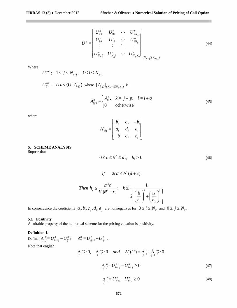
672

)1

)(1

(10

11110

00100

=

vN

xN

n

vN

xN

n

xN

n

xN

n

vN

nn

n

vN

nn

n

UUU

UUU

UUU

U

(44)

Where

11

1 1,1;

xv

n NiNjU

)(= )(

1 n

ij

nn

ij AUTrazaU where 1)1)(()( ][

xN

vN

n

ijA is

otherwise0

=,=,=)(

qilpjkAA

n

kln

ij (45)

where

iji

iii

iji

n

kl

beb

ada

bcb

A =)(

5. SCHEME ANALYSIS Supose that

0>;;0 1

* hdc (46)

)(2 cdcdIf

2

2

2

1

2

2

2

1;

][

hh

b

kck

chThen

In consecuence the coeficients jijii edcba ,,,, are nonnegatives for xNi 0 and vNj 0 .

5.1 Positivity A suitable property of the numerical scheme for the pricing equation is positivity.

Definition 1.

Define 1=n n n

j i j iji

U U ; n

ij

n

ij

n

i UU 1= .

Note that english

1

0, 0 ( ) = 0n n n n n

j i j i ii j j j

and U

1 1= 0n n n

j i j i ji

U U (47)

1 1= 0n n n

i ij ijj

U U (48)


673

Then, for our scheme it is true that

1 10; 0n n n n

j j i ii i j j

If (49)

and the restrictions (46) are met, one gets that for a nonegative payoff 0

ijU the numerical solution englishn

ijU is

nonegative for

Nn 0 , xNi 0 vNj 0 .

5.2 Monotonicity For the sake of clarity in the presentation we introduce the following definition of monotonicity-preserving numerical

scheme (see Xiao et. al (1996)).

Definition 2.

Consider the scheme 0=)( n

ijUW , LnJjIi ,, . where J and L are sets of nonnegative integers.

We say that the scheme is i-monotonicity-preserving if assuming that 0n

ji then it occurs that

1 0n

ji

. So it, is

j-monotonicity-preserving if 0n

ij then

1 0n

ij

.

Proposition 1. Under hypotheses (46) and (49) the numerical scheme (34) is i-monotonicity-preserving and

j-monotonicity-preserving, with Nn 0 , xNi 0 y vNj 0 .

Proof. Let us write

=)()()(= 1

11

1

1

11

1

n

ij

n

ij

n

ij

n

ji

n

ji

n

ji

n

ij

n

ji UUUUUUUU

n

jii

n

jii

n

jij

n

jii

n

jij

n

iji

n

iji

n

iji UaUbUeUdUcUbUaUb 2112111111111111(

n

ijj

n

iji

n

ijj

n

jii

n

jii

n

jii

n

ij

n

ji

n

ji

n

jii UeUdUcUbUaUbUUUUb 111111111121 ()()

)11111

n

ij

n

jii

n

jii

n

jii UUbUaUb (50)

after some algebraic procedures

1 1

1 1 1 1 1 1 11 1 1 1 1 1

=n n n n n n n n n n

i j ij i j j i j j i j j j j j ji i i i i i i i

U U b b a c e

1 1 1 11 1 1

2

(2 )2

n n n n n n n

i j j j j j j ji i i i i i i

kd ki k

h

(51)

Asumming (47) and (48) and from (34), one can easily show that

1 1 1 11 1 1 1

( ) ( ) 0.n n n n

i j j i j ji i i i

b b (52)

then 0.11

1

n

ij

n

ji UU ▀

In an analogous way result that 0.11

1

n

ij

n

ij UU

Then, the numerical scheme (34) is i-monotonicity-preserving and j-monotonicity-preserving, with

Nn 0 , xNi 0 y vNj 0 .

Corollary 1.


674

Under hypothesess (46) and (49) and the notation of last proposition, assuming that the payoff function f(x) is

nondecreasing and nonnegative with f(0)=0, then the scheme (34) is nondecreasing and nonnegative in ji, for each

time stage n .

5.3 Consistency Consistency of a numerical scheme with respect to a partial differential equation means that the exact solution of the

finite diference scheme aproximates the exact solution of the PDE (see Smith (1985)).

Theorem 1. For any fixed parameters, the scheme (34) is consistent with the partial differential equation.

Proof. Trivial by construction (See section 4).

5.4 Stability To analyse teh linear Von Neumann stability of the scheme (34)rewrite

])[(exp=),( 21 nkmkIAjiU nn (53)

where I is imaginary unit, nA is the amplitude at time level n ,

i

i

hk

2= are phases angles with wavelengths i ,

and mxi = y nvj = .

Then, n

n

A

A 1

=

the amplification factor satisfies

)](sin)(cos[)](sin)(cos[)(cos2)](sin)(sin[4= 2222121 vkIvkevkIvkcdxkavkxkb (54)

Thus

|)](sin)(cos[)](sin)(cos[)(cos2)](sin)(sin[4|lim 22221210,

vkIvkevkIvkcdxkavkxkbvx

(55)

jjii ecda 2= (56)

Is clear that the coefficients of the numerical scheme (34) are 1=2 jjii ecda .

1=2= jjii ecda (57)

Therefore, the scheme (34) is conditionally stable.

5.5 Convergence Finally using the Lax-Richtmyer equivalence theorem with the theorem 1 and condition (57)we can conclude

convergence of the scheme (34).

6. RESULTS In this section we check the properties of the proposed numerical scheme (34).

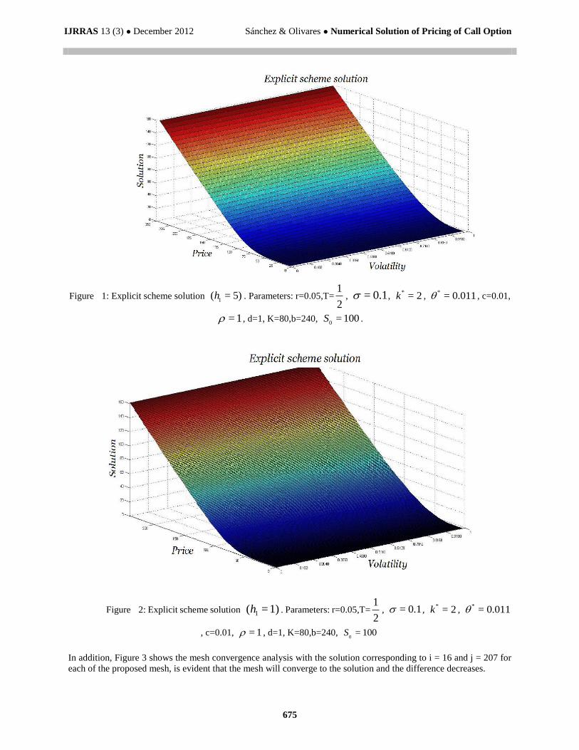
6.1 Example. Consider the european call option (so that f(s)=max(s-K,0)).

Figures show the computed price with numerical method, and the results obtained with 5=1h (Figure 1) and

1=1h (Figure 2).


675

Figure 1: Explicit scheme solution 1

( = 5)h . Parameters: r=0.05,T=2

1, 0.1= ,

*= 2k ,

*= 0.011 , c=0.01,

1= , d=1, K=80,b=240, 0

= 100S .

Figure 2: Explicit scheme solution 1)=( 1h . Parameters: r=0.05,T=2

1, = 0.1 ,

*= 2k ,

*= 0.011

, c=0.01, = 1 , d=1, K=80,b=240, 0

= 100S

In addition, Figure 3 shows the mesh convergence analysis with the solution corresponding to i = 16 and j = 207 for

each of the proposed mesh, is evident that the mesh will converge to the solution and the difference decreases.


676

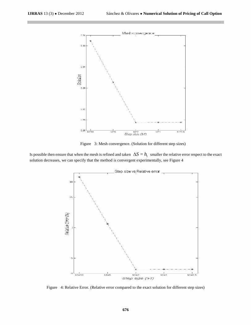
Figure 3: Mesh convergence. (Solution for different step sizes)

Is possible then ensure that when the mesh is refined and taken 1= hS smaller the relative error respect to the exact

solution decreases, we can specify that the method is convergent experimentally, see Figure 4

Figure 4: Relative Error. (Relative error compared to the exact solution for different step sizes)


677

7. CONCLUSIONS In this paper we have constructed a explicit finite difference numerical scheme that is consistent for the equation (28),

which was obtained by a transformation of variables in equation (12). The sufficient conditions for the step sizes of the

discretization in volatility and time are obtained depending on the step size of the asset price in order to ensure the

positivity of the coefficients and therefore of the solution in addition to stability of the scheme for general payment

convex functions. Our numerical scheme avoids inappropriate oscillations of the numerical solution because it is

monotonous - conservative.

The computational implementation of this numerical scheme is rather simple with a low computational cost and

provides desired solutions that are non-decreasing in the underlying asset and in the volatility direction from a

non-decreasing function of initial payments.

Some numerical computational results are performed to graphically illustrate the convergence of the scheme and the

approximation error.

REFERENCES [1]. B. Düring , M. Fournié, High-order compact finite difference scheme for option pricing in stochastic volatility

models, Journal of Computational and Applied Mathematics 236, 4462–4473, 2012

[2]. D.Y. Tangman, A. Gopaul, and M. Bhuruth. Numerical pricing of options using high- order compact finite

difference schemes. J. Comp. Appl. Math. 218(2), 270–280, 2008.

[3]. F. Black and M. Scholes. The pricing of options and corporate liabilities. J. Polit. Econ. 81, 637-659, 1973.

[4]. F. Xiao, T. Yabe, T. Ito, Constructing oscillation preventing scheme for advection equation by rational

function, Computer Physics Communications 29, 1-12, 1996.

[5]. González Rodríguez, Oscar. Extensión del Método de las Diferencias Finitasen el Dominio del Tiempo para el

Estudio de Estructuras Híbridas de Microondas Incluyendo Circuitos Concentrados Activos y Pasivos, PhD

Tesis. Universidad de Cantabria, 2008.

[6]. J.C. Strikwerda. Finite difference schemes and partial differential equations. Second edition. Society for

Industrial and Applied Mathematics (SIAM), Philadelphia, PA, 2004.

[7]. K. J. In 't Hout and S. Foulon. ADI finite difference schemes for option pricing in the Heston model with

correlation. International journal of numerical analysis and modeling volume 7, number 2, pages 303–320,

2010.

[8]. Mao, X. Stochastic differential equations and applications. Horwood publishing limited, Chichester, 1 edition,

1997.

[9]. R. Kangro, R. Nicolaides, Far field boundary conditions for Black_Scholes equations, SIAM Journal on

Numerical Analysis 38 (4),1357-1368, 2000.

[10]. S.L. Heston. A closed-form solution for options with stochastic volatility with applications to bond and

currency options. Review of Financial Studies 6(2), 327–343, 1993.

[11]. U.S. Rana, Asad Ahmad, Numerical solution of pricing of european option with stochastic volatility,

International Journal of Engineering 24 (2), 189–202, 2011.

Documents

NUMERICAL SOLUTION OF PRICING OF EUROPEAN CALL OPTION … · IJRRAS 13 (3) December 2012 Sánchez & Olivares Numerical Solution of Pricing of Call Option 667 In the mathematical literature,