Embed Size (px)
Citation preview

Technical report, IDE1113 , September 27, 2011
Master’s Thesis in Financial Mathematics
Elena Bukina
School of Information Science, Computer and Electrical EngineeringHalmstad University
Efficient Numerical Solution ofPIDEs in Option Pricing
Efficient Numerical Solution of PIDEsin Option Pricing
Elena Bukina
Halmstad University
Project Report IDE1113
Master’s thesis in Financial Mathematics, 15 ECTS credits
Supervisor: Prof. Dr. Matthias Ehrhardt
Examiner: Prof. Dr. Ljudmila A. Bordag
External referees: Prof. Mikhail Babich
September 27, 2011
Department of Mathematics, Physics and Electrical engineeringSchool of Information Science, Computer and Electrical Engineering
Halmstad University


Preface
I would like to express my gratitude to my supervisor prof. MatthiasEhrhardt and to the director of the program Ljudmila A. Bordag for theirhelp and advices in writing this thesis, this work would not exist withoutthem.

ii

Abstract
The estimation of the price of different kinds of options plays a veryimportant role in the development of strategies on financial and stockmarkets. There many books and various papers which are devoted tothe exist mathematical theory of option pricing. Merton and Scholesbecame winners of a Nobel Prize in economy who described the basicconcepts of the mathematical theory development.
In this thesis a review of the basic numerical methods for optionpricing including the treatment of jumps is given. These methods arecompared and numerical results are presented.
iii

iv
Contents
1 Introduction 1
2 Introduction To Robust Numerical Methods. 32.1 The Basic Model . . . . . . . . . . . . . . . . . . . . . . . . . 32.2 The Θ–Method Discretization . . . . . . . . . . . . . . . . . . 52.3 The Crank–Nicolson Discretization . . . . . . . . . . . . . . . 92.4 The Fixed–Point Iteration Method . . . . . . . . . . . . . . . 10
3 The Basic Numerical Methods For Option Pricing In TheModels With Jump–Diffusion. 133.1 The Basic Concepts About Fast Fourier Transformation (FFT) 143.2 Specifications of FFT . . . . . . . . . . . . . . . . . . . . . . . 16
4 A Numerical Example 19
5 Conclusions 27
Notation 29
Bibliography 31
Appendix 35
v

vi
Chapter 1
Introduction
Options are an important part of financial markets worldwide. The marketof futures and option contracts gained a popularity since its inception in 1973,when the trade of options and futures began on the Chicago Board OptionsExchange.
An option is a contract that gives to the buyer the right, but not theobligation, to buy or to sell an asset at a previous agreed strike price. Anoption contract with no special characteristics, which has a standard expirydate and strike price, contains no unusual provisions, is called a plain vanillaoption [1]. With the development of the market some additional conditionswere included in terms of option contracts. It was done in response to therequests from customers, who wished to hedge the risk.
Particularly successful inventions were offered on the market in droves.Thus the nonstandard options arose containing some provisions that makethem different from a straightforward option contracts with a strike price,underlying asset, and expiration date. Such options are called exotic options.Existing methods of evaluation options can be divided into two main groups.Classical models, e.g. ”Black–Scholes model”, value the price of options usingmathematically derived formulas. However, such models are limited in valu-ing exotic options. Therefore, it is necessary to use other methods. Numericalmethods, e.g. binomial methods, finite difference methods or Monte–Carlomethods, allow to value most exotic options and derivatives.
Eraker [3] showed that the usual assumption of ”geometric Brownian mo-tion” (GBM) should be improved by including discontinuous jump processes.Such models were originally introduced 1976 in the option valuation contextby Merton [4]. But most of them are confined to vanilla options. Therewas done a very little work on numerical methods for pricing exotic optionsbecause such techniques are required when jumps are combined with non-constant local volatilities.
1

2 Chapter 1. Introduction
In general, the valuation of options with jump diffusion processes requiressolving a ”partial integro–differential equation” (PIDE). Such equations arefunctional equations which involve both integrals and derivatives of a func-tion. This method was suggested 1993 by Amin [5].
An advantage of that method is that it can easily modify existing optionpricing software. Thus, a variety of exotic option contracts can be handledin a straightforward way.
The plan of this thesis is as follows. In this chapter the introduction of thenotion of financial derivatives is given. In Chapter 2 the robust numericalmethods are presented. The discretization of the Θ–method and Crank–Nicolson method are also considered. The fixed–point iteration method isdescribed and the convergence of the method is mentioned. Chapter 3 isabout the numerical method for option pricing in the jump–diffusion model.All results are presented in Chapter 4 and discussed and interpreted in Chap-ter 5. Finally, proofs of theoretical results and MATLAB program code maybe found in the Appendix.
Chapter 2
Introduction To RobustNumerical Methods.
2.1 The Basic Model
First, let us consider time period dt and let S will change by the law law
dS = µ(t)Sdt+ σ(t)SdW + (q(t)− 1)Sdp, (1)
where µ(t) = r(t)− d(t)− λ(t)k(t) is the drift rate, σ(t)is the volatility, dWis the increment of a continuous–time stochastic process, called a Wienerprocess, dp is a Poisson process [2]. k(t) = E(q(t) − 1), that depends fromt are identically independent distributed random variables representing theexpected relative jump size with k(t). Any k(t) that belong to an interval(−1,∞) for all t and q(t)− 1 is an impulse function producing a jump fromS to Sq(t). It is important that dp = 0 with probability 1− λdt and dp = 1with probability λdt, where λ is the Poisson arrival intensity, which is theexpected number of ”events” or ”arrivals” that occur per unit time.
Now let us consider a case, when dp = 0 in (1), then the given equationwill be equivalent to the usual stochastic process of ”geometric Brownianmotion” (GBM) assumed in the Black–Scholes models. If the Poisson eventoccurs, then equation (1) can be written as
dS
S' q(t)− 1, (2)
In this case the function q(t) − 1 is an impulse function producing a jumpfrom S to Sq(t).
Now we consider V (S, t) as the contingent claim depending of the assetprice S and time t. Let in equation (1) dt = 0. Then the following backward–
3
4 Chapter 2. Introduction To Robust Numerical Methods.
in–time ”partial integro–differential equation” (PIDE) may be solved to de-termine V :
∂V
∂t+ µ(t)S
∂V
∂S+
1
2σ2S2∂
2V
∂S2+ λE[∆V ]− rV = 0, (3)
where E[∆V ] can be presented in the following form
E[∆V = E[V ]− V =
∞∫0
V (Sq)g(q)dq − V,
and E[·] is the expectation operator for the given equation.Next we can apply the reversal time τ = T − t, µ(τ) = r(τ)− λ(τ)k(τ),
where T is the expiry time of the contingent claim and r is the continuouslycompounded risk–free interest rate, and g(q) is the probability density func-tion of the jump amplitude q with the properties that for all q, g(q) ≥ 0. Incase when the jump size is log–normally distributed, the probability densityfunction reads
g(q) =exp
{− (log(q)−ν)2
2%2
}√
2π%q,
where ν is the mean and %2 is the variance of the jump size probabilitydistribution. It is possible to present the expectation operator in the formE[q(t)] = exp
{ν + %
2
}, i.e.
k(τ) = E[q(τ)− 1] = exp
{ν +
%2
2
}− 1.
This allows us to write the following partial integro–differential equationas
∂V
∂τ= µ(τ)S
∂V
∂S+
1
2σ2S2∂
2V
∂S2+ λ
∞∫0
V (Sq)g(q)dq − (λ− r)V, (4)
which is supplied with the following
Boundary conditions. [4]
As the asset price S → 0, the equation (4) converges to
∂V
∂τ= −rV. (5)
If S →∞, we can assume that
Efficient Numerical Solution of PIDEs 5
∂2V
∂S2' 0, (6)
This equation means that
V ' A(τ)S +B(τ). (7)
This condition is called a Dirichlet condition which can be determined by theoption payoff. If (7) holds, then (4) reduces to
∂V
∂τ=
1
2σ2S2∂
2V
∂S2+ rS
∂V
∂S− rV. (8)
Thus, when S = 0 and S → ∞, then PIDE (4) reduces to the Black–Scholes PDE, and the usual boundary conditions can be imposed.
2.2 The Θ–Method Discretization
In this section we consider θ–method sampling for PIDE without jumpintegral terms. Thus, we reformulate the integral (4) as a correlation integralfor efficiency.
To begin with let us consider
I(S) =
∞∫0
V (Sq)g(q)dq. (9)
Assuming that x = log(S) and y = log(q) we get the following
I(S) =
∞∫−∞
V (ex+y)g(ey)dey =
∞∫−∞
V (x+ y)f(y)dy, (10)
where V (ex+y) = V (x + y), g(ey)ey = f(y) and f(y) is the probability com-pactness function of a jump of size y = log(q). Equation (10) also can be likeV ⊗ f , as it corresponds to the interdependence product of V (y) and f(y).Let us recall that the discrete form of integral (10) is
Ii =
j=N/2∑j=−N/2+1
V i+jf j∆y +O((∆y)2), (11)
where Ii = I(i∆x), V j = V (j∆x),
6 Chapter 2. Introduction To Robust Numerical Methods.
f j =1
∆x
xj+∆x/2∫xj−∆x/2
f(x)dx. (12)
It is assumed that xj = j∆x, ∆x = ∆y and N is large enough such that thesolution in areas of interest can be approximated by using an asymptoticboundary condition for large values of S. Note, that f(y) extensionallydefined by (12) is a probability density function [6], thus, it possesses anessential property
j=N/2∑j=−N/2+1
f j∆y ≤ 1, f j ≥ 0, ∀j. (13)
Let us try to use the unequal distribution of S coordinates in the grid forthe PDE discretization. Assume
V ni = V (Si, τn), (14)
where V j will not certainly correspond necessarily with any of the discretevalues Vi in (14). Applying Lagrange basis functions defined on the S gridwe can conclude that, if
Sγ(j) ≤ ej∆x ≤ Sγ(j)+1, (15)
then it is possible to write down as
V j = ψγ(j)Vγ(j) + (1− ψγ(j))Vγ(j)+1 +O((∆Sγ(j)+1/2)2), (16)
where γ(j), ψγ(j) are interpolation weights [7], and ∆Si+1/2 = Si+1 − Si.If exΠ(k) ≤ Sk ≤ ex
∏(k)+1, then we obtain
I(Sk) = φΠ(k)IΠ(k) + (1− φΠ(k))IΠ(k)+1 +O((exΠ(k) − exΠ(k)+1)2), (17)
where φΠ(k) is an interpolation weight and 0 ≤ φi ≤ 1, 0 ≤ ψi ≤ 1.Combining (11), (16), (17) we get
I(Sk) =
j=N/2∑j=−N/2+1
ξ(V, k, j)f j∆y, (18)
where V = [V0, V1, ..., Vp]′ and
ξ(V, k, j) = φΠ(k)[ψγ(k)+jVγ(Π(k)+j) + (1− ψγ(Π(k)+j))Vγ(Π(k)+j)+1]

Efficient Numerical Solution of PIDEs 7
+(1− φΠ(k))[ψγ(Π(k)+1+j)Vγ(Π(k)+1+j) + (1− ψγ(Π(k)+1+j)+1)]. (19)
Also notice that ξ(V, k, j) is linear in V , then it follows ξ(1, k, j) = 1 for allk, j.
Now we can use an implicit method for PDE, and then we use a weightedtime discretization, obtaining a method for computing the jump integral. Wewill rewrite the discrete equation in a following form
V n+1i [1 + (αi + βi + r + λ)∆τ ]−∆τβiV
n+1i+1 −∆ταiV
n+1i−1
= V ni + (1− θ)∆τλ
j=N/2∑j=−N/2+1
ξ(V n+1, i, j)f j∆y
+θ∆τλj=N/2∑
j=−N/2+1
ξ(V n, i, j)f j∆y,
(20)
where θ = 0 and θ = 1 are weighting parameters coinciding to an implicithandling of the jump integral and explicit treatment of this term respectively.
In common, discretizing the first derivative term of (4) with central dif-ferences leads to
αci =σ2S2
i
(Si−Si−1)(Si+1−Si−1)− (r−λk)Si
Si+1−Si−1,
βci =σ2S2
i
(Si+1−Si)(Si+1−Si−1)+ (r−λk)Si
Si+1−Si−1,
(21)
and if αci ≤ 0 or βci ≤ 0, oscillations may appear in the numeric solution.These can be avoided by applying forward or backward differences at theproblem nodes, leading to forward difference [9]
αfi =σ2S2
i
(Si−Si−1)(Si+1−Si−1),
βfi =σ2S2
i
(Si+1−Si)(Si+1−Si−1)+ (r−λk)Si
Si+1−Si ,(22)
or backward difference
αbi =σ2S2
i
(Si−Si−1)(Si+1−Si−1)− (r−λk)Si
Si−Si−1,
βbi =σ2S2
i
(Si+1−Si)(Si+1−Si−1).
(23)
We can choose between the forward and the backward differences usingthis algorithm [12].
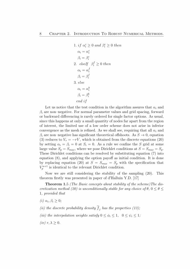
8 Chapter 2. Introduction To Robust Numerical Methods.
1. if αci ≥ 0 and βci ≥ 0 then
αi = αci
βi = βci
2. elseIf βfi ≥ 0 then
αi = αfi
βi = βfi
3. else
αi = αbi
βi = βbi
end if
Let us notice that the test condition in the algorithm assures that αi andβi are non–negative. For normal parameter values and grid spacing, forwardor backward differencing is rarely ordered for single factor options. As usual,since this happens at only a small quantity of nodes far apart from the regionof interest, the limited use of a low order scheme does not arise in inferiorconvergence as the mesh is refined. As we shall see, requiring that all αi andβi are non–negative has significant theoretical offshoots. As S → 0, equation(3) reduces to Vτ = −rV , which is obtained from the discrete equations (20)by setting αi = βi = 0 at Si = 0. As a rule we confine the S grid at somelarge value Sp = Smax, where we pose Dirichlet conditions at S = Smax = Sp.These Dirichlet conditions can be resolved by substituting equation (7) intoequation (8), and applying the option payoff as initial condition. It is doneby replacing equation (20) at S = Smax = Sp with the specification thatV n+1p is identical to the relevant Dirichlet condition.
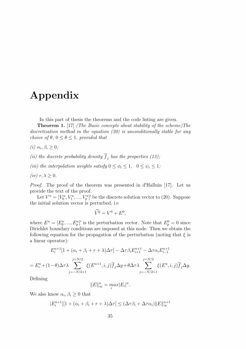
Now we are still considering the stability of the sampling (20). Thistheorem firstly was presented in paper of d′Halluin Y.D. [17]
Theorem 1.5 (The Basic concepts about stability of the scheme)The dis-cretization method (20) is unconditionally stable for any choice of θ, 0 ≤ θ ≤1, provided that
(i) αi, βi ≥ 0;
(ii) the discrete probability density f j has the properties (13);
(iii) the interpolation weights satisfy 0 ≤ φi ≤ 1, 0 ≤ ψi ≤ 1;
(iv) r, λ ≥ 0.
Efficient Numerical Solution of PIDEs 9
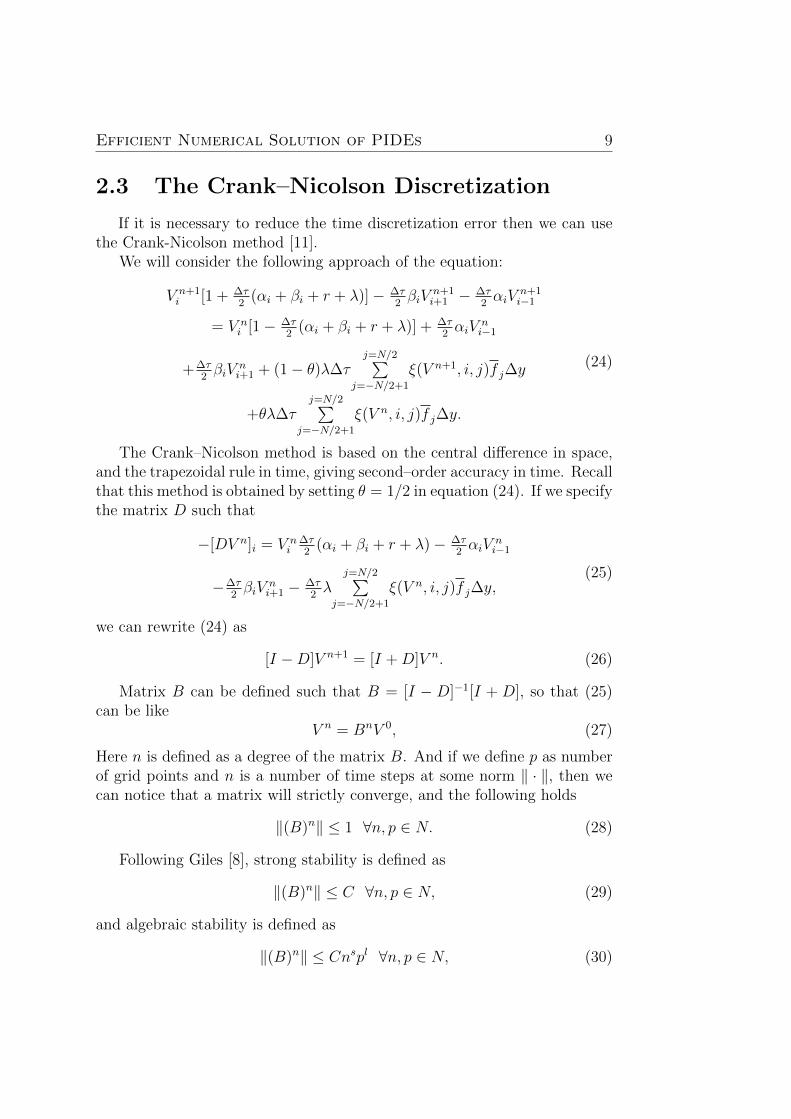
2.3 The Crank–Nicolson Discretization
If it is necessary to reduce the time discretization error then we can usethe Crank-Nicolson method [11].
We will consider the following approach of the equation:
V n+1i [1 + ∆τ
2(αi + βi + r + λ)]− ∆τ
2βiV
n+1i+1 − ∆τ
2αiV
n+1i−1
= V ni [1− ∆τ
2(αi + βi + r + λ)] + ∆τ
2αiV
ni−1
+∆τ2βiV
ni+1 + (1− θ)λ∆τ
j=N/2∑j=−N/2+1
ξ(V n+1, i, j)f j∆y
+θλ∆τj=N/2∑
j=−N/2+1
ξ(V n, i, j)f j∆y.
(24)
The Crank–Nicolson method is based on the central difference in space,and the trapezoidal rule in time, giving second–order accuracy in time. Recallthat this method is obtained by setting θ = 1/2 in equation (24). If we specifythe matrix D such that
−[DV n]i = V ni
∆τ2
(αi + βi + r + λ)− ∆τ2αiV
ni−1
−∆τ2βiV
ni+1 − ∆τ
2λ
j=N/2∑j=−N/2+1
ξ(V n, i, j)f j∆y,(25)
we can rewrite (24) as
[I −D]V n+1 = [I +D]V n. (26)
Matrix B can be defined such that B = [I − D]−1[I + D], so that (25)can be like
V n = BnV 0, (27)
Here n is defined as a degree of the matrix B. And if we define p as numberof grid points and n is a number of time steps at some norm ‖ · ‖, then wecan notice that a matrix will strictly converge, and the following holds
‖(B)n‖ ≤ 1 ∀n, p ∈ N. (28)
Following Giles [8], strong stability is defined as
‖(B)n‖ ≤ C ∀n, p ∈ N, (29)
and algebraic stability is defined as
‖(B)n‖ ≤ Cnspl ∀n, p ∈ N, (30)

10 Chapter 2. Introduction To Robust Numerical Methods.
where C, s and l ≥ 0 are constants independent of n and p.Algebraic stability is a weaker condition than either strict or strong stabil-
ity. The Lax Equivalence Theorem states that strong stability is an essentialand sufficient condition for convergence for all initial data.
If we assume that µi is an eigenvalue of D then a necessary conditionfor strong stability is given by |µi| ≤ 1 and |µi| = 1 that should have thefrequency rate is equal to 1. From equation (25) and properties (13), we havethe following
• All diagonals of D are non–negative;
• All diagonals of D (except the last row) should be strictly negative;
• Assuming that r > 0 andj=p∑j=0
Dij < 0 for i = 0, ..., p− 1;
• The last row of D should be identically equal to zero because of Dirich-let conditions.
According to the assumptions made above we can conclude that the ma-trix D is strictly contained in the negative part of a complex plane with oneeigenvector which is equal to zero. Thus, all eigenvectors of B are equal orless than 1, except one which modulus is equal to 1. And the matrix Bsatisfies to all necessary conditions for strict stability. On the other hand,B is not a symmetric matrix, thereby it is not enough conditions for itsbound. In that case the algebraic stability can be guaranteed by checkingthe eigenvalues µi of matrix D.
2.4 The Fixed–Point Iteration Method
If you use an implicit discretization, it is computationally prohibited toresolve the full linear system because the correlation product term makesthe system dense. Therefore, we suppose the use of a fixed–point iterationto solve the linear system.
Now we consider a matrix D such that
−[DV n]i = V ni ∆τ(αi + βi + r + λ)− V n
i−1∆ταi − V ni+1∆τβi. (31)
It is also necessary to define a vector Φ(V n) which is a linear function of V n
that looks like
[Φ(V n)]i =
j=N/2∑j=−N/2+1
ξ(V n, i, j)f j∆y. (32)
Efficient Numerical Solution of PIDEs 11
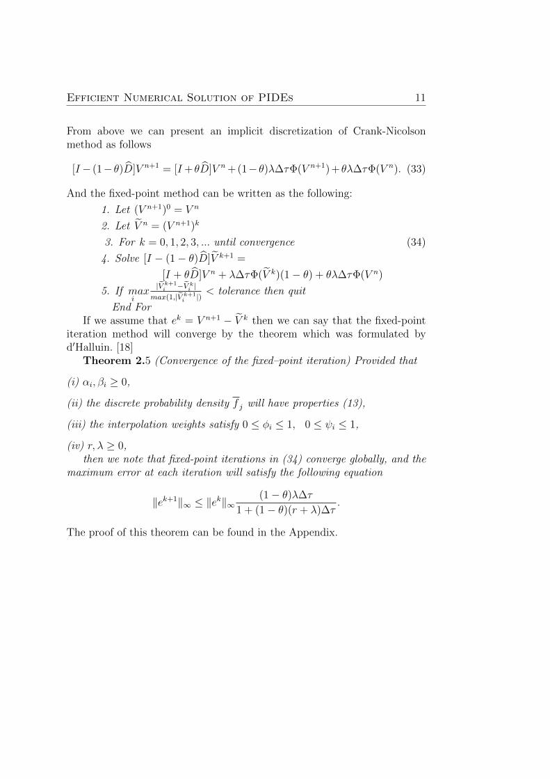
From above we can present an implicit discretization of Crank-Nicolsonmethod as follows
[I− (1− θ)D]V n+1 = [I+ θD]V n+ (1− θ)λ∆τΦ(V n+1) + θλ∆τΦ(V n). (33)
And the fixed-point method can be written as the following:
1. Let (V n+1)0 = V n
2. Let V n = (V n+1)k
3. For k = 0, 1, 2, 3, ... until convergence (34)
4. Solve [I − (1− θ)D]V k+1 =
[I + θD]V n + λ∆τΦ(V k)(1− θ) + θλ∆τΦ(V n)
5. If miax
|V k+1i −V ki |
max(1,|V k+1i |)
< tolerance then quit
End ForIf we assume that ek = V n+1 − V k then we can say that the fixed-point
iteration method will converge by the theorem which was formulated byd′Halluin. [18]
Theorem 2.5 (Convergence of the fixed–point iteration) Provided that
(i) αi, βi ≥ 0,
(ii) the discrete probability density f j will have properties (13),
(iii) the interpolation weights satisfy 0 ≤ φi ≤ 1, 0 ≤ ψi ≤ 1,
(iv) r, λ ≥ 0,then we note that fixed-point iterations in (34) converge globally, and the
maximum error at each iteration will satisfy the following equation
‖ek+1‖∞ ≤ ‖ek‖∞(1− θ)λ∆τ
1 + (1− θ)(r + λ)∆τ.
The proof of this theorem can be found in the Appendix.

12 Chapter 2. Introduction To Robust Numerical Methods.

Chapter 3
The Basic Numerical MethodsFor Option Pricing In TheModels With Jump–Diffusion.
Now we should develop the numerical methods for correct and rationalestimation of the option price in order to use the model described above inpractice. These methods should satisfy to integro-differential equation (3).The main goal is also to find numerical solution of (4) which can usually arisein iterative methods of calibration.
Thereupon there is not enough papers connected with numerical methodsfor a finding of the decision integro-differential the equation in private deriva-tives in models with diffusive jump. Such models were used and describedAmin [5] Thereupon, there is a sufficiently small number of papers related tonumerical methods that find solutions of partial integro-differential equationsin models with a diffusion jump. Such models were used and described byAmin [5] and Andreasen and Gruenewald [13].
Such methods, known as explicit, have unstable time convergence. Thus,implicit methods are much more accurate and stable in comparison withexplicit ones. And therefore they are preferable for option pricing.
There are different papers that describe the use of implicit methods, thatcan determine the solution of the partial integro–differential equation. Butsuch methods are used for the finite-difference Crank-Nicolson scheme, andthis approach assumes that finding the unknown elements of the matrix oc-curs at each time step. So, this method can be used for option pricing, butfinding the elements in this way is inefficient, and that’s why it is necessaryto use another approach.
There are works in which implicit methods and which are capable tosolve the partial integro–differential equation are used, but such methods
13
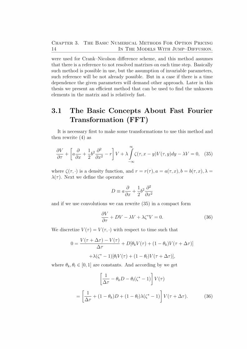
14Chapter 3. The Basic Numerical Methods For Option Pricing
In The Models With Jump–Diffusion.
were used for Crank–Nicolson difference scheme, and this method assumesthat there is a reference to not resolved matrixes on each time step. Basicallysuch method is possible in use, but the assumption of invariable parameters,such reference will be not already possible. But in a case if there is a timedependence the given parameters will demand other approach. Later in thisthesis we present an efficient method that can be used to find the unknownelements in the matrix and is relatively fast.
3.1 The Basic Concepts About Fast Fourier
Transformation (FFT)
It is necessary first to make some transformations to use this method andthen rewrite (4) as
∂V
∂τ+
[a∂
∂x+
1
2b2 ∂
2
∂x2− r]V + λ
∞∫−∞
ζ(τ, x− y)V (τ, y)dy − λV = 0, (35)
where ζ(τ, ·) is a density function, and r = r(τ), a = a(τ, x), b = b(τ, x), λ =λ(τ). Next we define the operator
D ≡ a∂
∂x+
1
2b2 ∂
2
∂x2
and if we use convolutions we can rewrite (35) in a compact form
∂V
∂τ+DV − λV + λζ∗V = 0. (36)
We discretize V (τ) = V (τ, ·) with respect to time such that
0 =V (τ + ∆τ)− V (τ)
∆τ+D[θkV (τ) + (1− θk)V (τ + ∆τ)]
+λ(ζ∗ − 1)[θlV (τ) + (1− θl)V (τ + ∆τ)],
where θk, θl ∈ [0, 1] are constants. And according by we get[1
∆τ− θkD − θl(ζ∗ − 1)
]V (τ)
=
[1
∆τ+ (1− θk)D + (1− θl)λ(ζ∗ − 1)
]V (τ + ∆τ). (36)
Efficient Numerical Solution of PIDEs 15
We have mentioned earlier, that there are different numerical methods todetermine the numerical solution of (36). We may use here the Crank–Nicolson finite difference scheme with parameters θk = θl = 1
2, but such use
is not entirely correct in this case. We need to treat to a matrix of size N×Nafter sampling the space of coordinates x by the number of points of N . Andit is very inconvenient, since it has N3 computational costs. But we have seenthat such approach of the matrix treatment must be done at each time step,because its elements are not constant and we are not allowed to use the FFT.Then we should try the schemes, where the parameters θk = 1
2, θl = 0 [15].
These schemes are not only stable but also effective. However, the stabil-ity decreases because of the asymptotic representation of discrete and con-tinuous parts. Then we will use an implicit method of alternating directions.This is a method where each time step in the grid will be divided into twohalf–steps. For the first half–step we have θk = 1, θl = 0, and then we get.[
1
∆τ/2−D
]V (t+ ∆) =
[1
∆τ/2− λ+ λς∗
]V (τ + ∆τ). (37)
In a discrete grid we can solve this by first computing the convolution ζ∗V (τ+∆τ) in discrete Fourier space, where
〈ς∗V (τ + ∆τ)〉 = 〈ς〉〈V (τ + ∆τ)〉.
When we notice that ζ only needs to be computed once, the computationalcosts associated with the convolution part of (37) is one FFT and one in-verse FFT, i.e. O(Nlog2N). Then we note that the discrete version of thedifferential operator D is a tridiagonal matrix. Therefore, once the RHS of(37) is acquired by FFT methods, then we can resolve the system (37) at acost of O(N). Consequently, the total costs of solving (37) is O(Nlog2N).
We get the second half step if θk = 0, θl = 1, then we have[1
∆τ/2+ λ− λζ∗
]V (τ) =
[1
∆τ/2+D
]V (τ +
∆τ
2). (38)
If we assume that y = [ 2∆τ
+D]V (t+ ∆τ2
) then we can apply FFT to (38).
(2
∆τ+ λ)〈V (τ)〉 − λ〈ζ〉〈V (τ)〉 = 〈y〉
〈V (τ)〉 =〈y〉
( 2∆τ
) + λ− λ〈ζ〉(39)
We need to define the following operators for the discrete scheme (37)and (38)
δxf(x) =1
2∆x[f(x+ ∆x)− f(x−∆x)] ,

16Chapter 3. The Basic Numerical Methods For Option Pricing
In The Models With Jump–Diffusion.
δxxf(x) =1
(∆x)2[f(x+ ∆x)− 2f(x) + f(x−∆x)] ,
Df(x) =
[aδx +
1
2b2δxx
]f(x);
f(x)ζ∗
=∑j
qj(x)f(j∆x),
where
qj(x) =
(j+ 12
)∆x∫(j− 1
2)∆x
ζ(x− y)dy.
Also we can present (37) and (38) in discrete form.[2
∆τ−D
]V
(τ +
∆τ
2
)=
[2
∆τ− λ+ λζ
∗]V (τ + ∆τ), (40)
[2
∆τ+ λ− λζ∗
]V (τ) =
[2
∆τ+D
]V
(τ +
∆τ
2
). (41)
The next assumption describes the properties of schemes (40), (41).
Proposition 1.5The given properties are necessary for schemes (40),(41):
(i) The given schemes are unconditionally stable in the von Neumann sense.
(ii) If the parameters are known, then the numerical solution will be locallystable and has O(∆τ 2 + ∆x2) order of accuracy.
(iii) If M is a number of time steps, N is the number of space steps, thenthe order of accuracy will be O(MNlog2N)
3.2 Specifications of FFT
The scheme (40) and (41) is convenient for finding the numerical solution:it is unconditionally stable and has O(Nlog2N) order of accuracy. Alsonote that it is important to make correct representation of the convolutionintegral. And if FFT uses steps with identical length then the accuracy ofthe solution will be low in areas of interest. To avoid such a problem, we
Efficient Numerical Solution of PIDEs 17
have made the assumption in the algorithm that the linear part of an optionwill be equal to a number of standard deviations from the basic process outof a grid. Then the linear part should be solved in the closed form, and thesolution can be found on an inner grid by FFT algorithm [15]
It is necessary to divide function into two parts. So, it turns out
V = V 1x∈(x,x) + V 1x/∈(x,x) ≡ G+H,
On x ∈ (x, x), G, then we have
∂G
∂τ+DG+ λ(ζ∗ − 1)V =
∂G
∂τ+DG− λG+ λζ∗[G+H].
If we assume that H is linear in ex we can write
H(τ, x) ∼= [gl(τ)ex + hl(τ)]1x<x + [gu(τ)ex + hu(τ)]1x>x,
where gl, gu, hl, hu are deterministic functions. It means that
ζ∗H(τ, x) ∼= gl(τ)ex(1 +m(t))Pr′(x+ lnJ(τ) < x)
+hl(τ)Pr(x+ lnJ(l) < x)
+gu(τ)ex(1 +m(l))Pr′(x+ lnJ(l) > x)
+hu(τ)Pr(x+ lnJ(τ) > x) (42)
where Pr(·) is a probability in sense of distribution which defines ζ and Pr′(·)is a Radon-Nikodim distrubution [14] represented as
ζ ′(τ, x) =ζ(τ, x)ex
(1 +m(τ)).
As for lognormaly distributed jump (Merton [4]) we can evaluate the givenprobabilities in the closed form like function of Gaussian distribution. But ifjump distributions are not set parametrical then we consider probability byelementary numerical integration on a plane ζ, ζ ′. And then we obtain[
2
∆τ−D
]G(τ +
∆τ
2) = (
2
∆τ− λ)G(τ + ∆τ) + λζ∗G(τ + ∆τ)
+λζ∗H(τ + ∆τ),
[2
∆τ+ λ− λζ∗
]G(τ)
=
[2
∆τ+D
]G
(τ +
∆τ
2
)+ λζ∗H(τ), (43)
18Chapter 3. The Basic Numerical Methods For Option Pricing
In The Models With Jump–Diffusion.
where ζ∗G can be numerically evaluated by FFT, and ζ∗G can be found from(42). We assumed that H is a linear function and then functions gl, gu, hl, hucan be written as
rf = fτ + (r(τ)− g(τ))fx. (44)
For discrete time distribution (44) we have
f(τ, x) = e−r∆τf(τ + ∆τ, x+ (r(τ)− q(τ))∆τ). (45)
together with the boundary conditions this define gl, gu, hl, hu.Now we use the above assumptions for various methods and programs,
even for options with barriers and the American options.
Chapter 4
A Numerical Example
In the two previous chapters we described the numerical methods used forevaluating the partial integro–differential equation which arise, as the equa-tions for option pricing with jump diffusion processes. We mentioned twovarious approaches to evaluate the correlation integral, FFT and the alter-native approach with a vector Φ(V N) which is a linear function of V N . Inthis chapter results which were obtained by applying the numerical methodwith different approaches are shown. For numerical experiments we took thefollowing parameters:
Parametersr = 0.2 interest rate K = 100 strike pricevol = 0.3 volatility σ T = 0.25 maturity timew = 0.5 weighting coefficient θ lam = 1 Poisson arrival intensity λnu = 0 mean ν g = 1 variance γphi = 0.5 weighting coefficient φ psi = 0.5 weighting coefficient ψ
Numerical Results for European Vanilla Call Option.
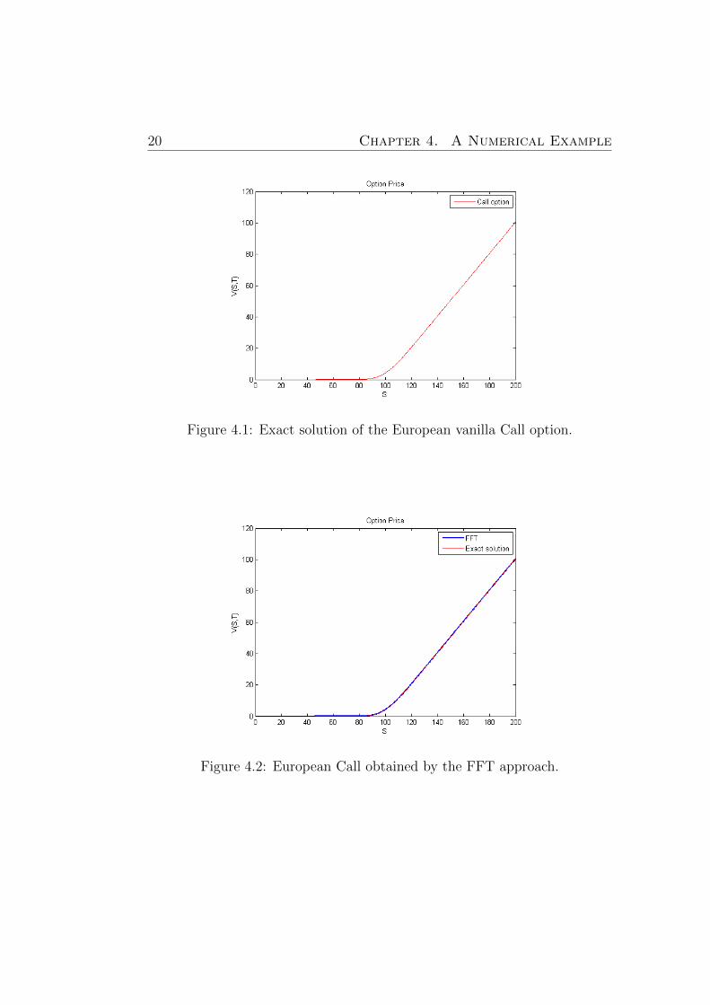
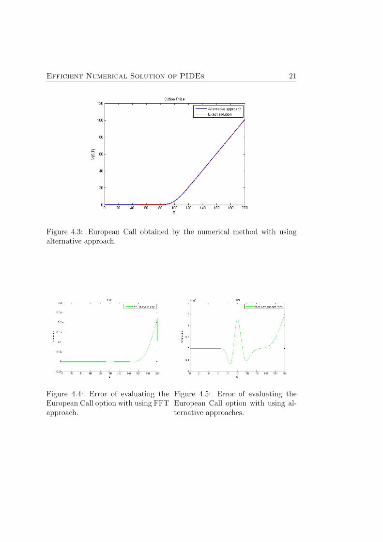
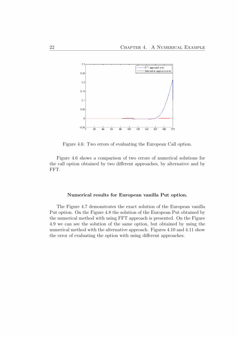
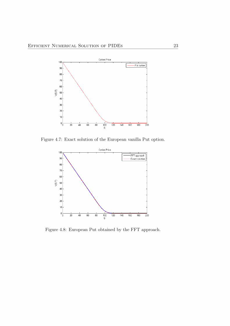
On the Figure 4.1 the exact solution of the European vanilla Call optionis presented. The Figure 4.2 demonstrates the solution of the European Callobtained by the numerical method with using FFT approach. On the Figure4.3 we can see the solution of the same option, but obtained by using the nu-merical method with the alternative approach. Figures 4.4 and 4.5 illustratethe error of evaluating the option with using different approaches.
19
20 Chapter 4. A Numerical Example
Figure 4.1: Exact solution of the European vanilla Call option.
Figure 4.2: European Call obtained by the FFT approach.
Efficient Numerical Solution of PIDEs 21
Figure 4.3: European Call obtained by the numerical method with usingalternative approach.
Figure 4.4: Error of evaluating theEuropean Call option with using FFTapproach.
Figure 4.5: Error of evaluating theEuropean Call option with using al-ternative approaches.
22 Chapter 4. A Numerical Example
Figure 4.6: Two errors of evaluating the European Call option.
Figure 4.6 shows a comparison of two errors of numerical solutions forthe call option obtained by two different approaches, by alternative and byFFT.
Numerical results for European vanilla Put option.
The Figure 4.7 demonstrates the exact solution of the European vanillaPut option. On the Figure 4.8 the solution of the European Put obtained bythe numerical method with using FFT approach is presented. On the Figure4.9 we can see the solution of the same option, but obtained by using thenumerical method with the alternative approach. Figures 4.10 and 4.11 showthe error of evaluating the option with using different approaches.
Efficient Numerical Solution of PIDEs 23
Figure 4.7: Exact solution of the European vanilla Put option.
Figure 4.8: European Put obtained by the FFT approach.
24 Chapter 4. A Numerical Example
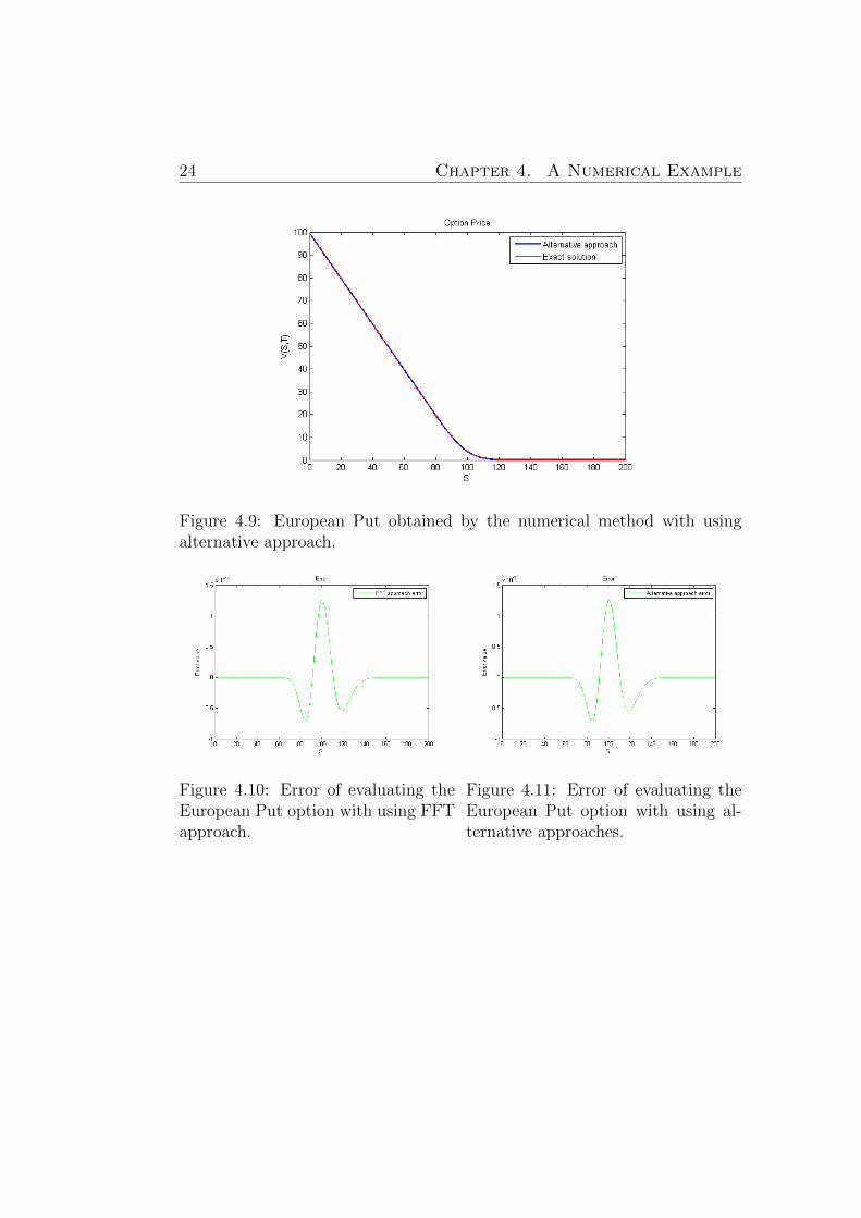
Figure 4.9: European Put obtained by the numerical method with usingalternative approach.
Figure 4.10: Error of evaluating theEuropean Put option with using FFTapproach.
Figure 4.11: Error of evaluating theEuropean Put option with using al-ternative approaches.
Efficient Numerical Solution of PIDEs 25
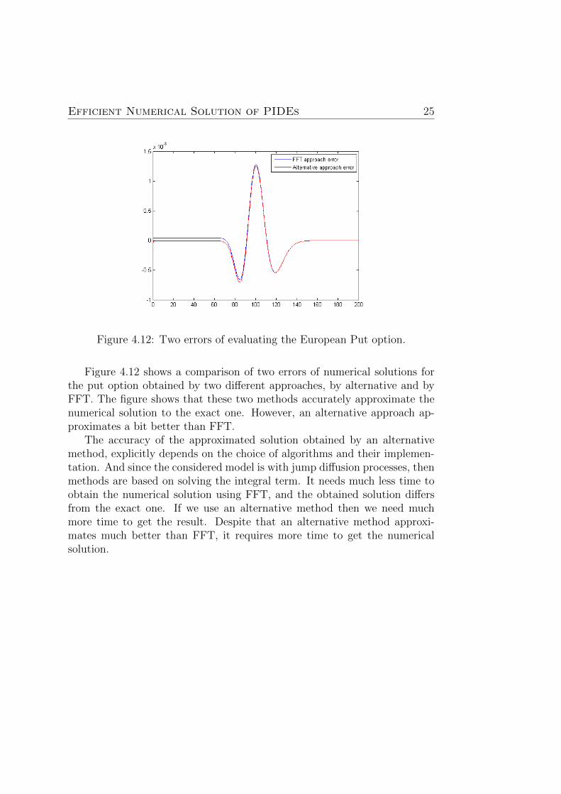
Figure 4.12: Two errors of evaluating the European Put option.
Figure 4.12 shows a comparison of two errors of numerical solutions forthe put option obtained by two different approaches, by alternative and byFFT. The figure shows that these two methods accurately approximate thenumerical solution to the exact one. However, an alternative approach ap-proximates a bit better than FFT.
The accuracy of the approximated solution obtained by an alternativemethod, explicitly depends on the choice of algorithms and their implemen-tation. And since the considered model is with jump diffusion processes, thenmethods are based on solving the integral term. It needs much less time toobtain the numerical solution using FFT, and the obtained solution differsfrom the exact one. If we use an alternative method then we need muchmore time to get the result. Despite that an alternative method approxi-mates much better than FFT, it requires more time to get the numericalsolution.

26 Chapter 4. A Numerical Example
Chapter 5
Conclusions
In this thesis we consider basic methods for finding the solution of thepartial integro–differential equations. Here both implicit and explicit meth-ods were described. It is done as the explicit method for the valuation ofthe correlation integral with the implicit PDE discretization becomes stable.But as this method has the first order of accuracy then it is better to use animplicit method and in this case there is decided to use the Crank–Nicolsonmethod. There is an algebraic stability of this method was proved, and thestability by the norm l2 is prooved also when grid S is equally distributed.
We suppose that the using of implicit time steps will lead to the factthat the direct estimation of the correlation integral is included in PIDEand then the solution of the dense matrix is required. In order to avoidthese calculations we use the fixed–point iteration method. It converges veryquickly, and each fixed point requires the correlation integral estimation.
Next we use the FFT approach to evaluate the correlation integral presentan alternative approach by the linear function.
As the given method is developed for financial tools with jump diffusionprocesses then it suites for a finding the price for American and exotic optionsalso.
The described methods were applied to find the price of European vanillaoptions and programmed in MATLAB. Finally, all numerical results werepresented and concisely.
27

28 Chapter 5. Conclusions
Notation
V (S, t) Price of opton
S Price of an asset
S0 Initial price of an asset
t Forward time
T Maturity date
τ Reversal time
r(t) Interest rate
σ(t) Volatility
K Strike price
N Number of the time steps
µ(t) Drift rate
dW Wiener process
dp Poisson process
λ(t) Poisson arrival intensity
k(t) Expected relative jump size
q(t) Impulse function
g(q(t)) Probability Density Function of q(t)
ν Mean
%2 Variance
E[·] Expectation operator
θ Weight parameter
γ(j), ψγ(j), φΠ(k) Interpolation weights
29

30
Bibliography
[1] http://en.wikipedia.org/wiki/Option–(finance) (2011)
[2] http://en.wikipedia.org/wiki/Stochastic–process (2011)
[3] B. Eraker, M. Johannes and N. Polson (2003)The impact of jumps in volatility and returns. J. Finance, 58, 1269 –1300.
[4] R. C. Merton (1976)Option pricing when underlying stock returns are discontinuous. J. Fi-nancial Econ., 3, 125 – 144.
[5] K. I. Amin (1993)Jump diffusion option valuation in discrete time. J. Finance, 48, 1833 –1863.
[6] http://http://en.wikipedia.org/wiki/Probability–density–function(2011)
[7] http://www.ems–i.com/gmshelp/Interpolation/Interpolation–Schemes/Inverse–Distance–Weighted/ Computation–of–Interpolation–Weights.htm (2011)
[8] M. B. Giles (1997)On the stability and convergence of discretizations of initial value PDEs.IMA J. Numer. Anal., 17, 563 – 576.
[9] http://en.wikipedia.org/wiki/Backward–differentiation–formula(2011)
[10] X. L. Zhang (1997)Numerical analysis of American option pricing in a jump–diffusionmodel. Math. Oper. Res., 22, 668 – 690.
[11] http://en.wikipedia.org/wiki/Crank–Nicolson–method (2011)
31
[12] http://en.wikipedia.org/wiki/Finite–difference–method (2011)
[13] J. Andreasen and B. Gruenewald (1996)American Option Pricing in the Jump-Diffusion Model. WorkingPaper,(http://www.cmap.polytechnique.fr/∼rama/dea/andreasen.pdf),Aarhus University and University of Mainz.
[14] http://en.wikipedia.org/wiki/Radon-Nikodym-heorem (2011)
[15] J. Andreasen (2000)American Option Pricing in the Jump-Diffusion Model. Review ofDerivatives Research, 4, 231–262, .
[16] A. Mitchell, and D. F. Griffiths (1980)The Finite Difference Method in Partial Differential Equations. Wileyand Sons.
[17] Y. d’Halluin, P.A. Forsyth and K.R. Vetzal (2005)Robust Numerical Methods for Contingent Claims under Jump DiffusionProcesses. IMA J. on Num. Anal., 25, 87–112.
[18] Y. d’Halluin, P.A. Forsyth and K.R. Vetzal (2004)Numerical Methods for Real Optionsin Telecommunications. Working Pa-per,(http://uwspace.uwaterloo.ca/bitstream/10012/1206/1/ydhallui2004.pdf),Waterloo, Ontario, Canada.
[19] A. Mayo (2008)Methods for the rapid solution of the pricing PIDEs in exponential andMerton models. J. Comput. Appl. Math., 222, 128–143.
[20] C. Johnson (1987)Numerical Solutions of Partial Differential Equations by the Finite Ele-ment Method. Cambridge University Press.
[21] C. Anderson and M.D. Dahleh (1996)Rapid computation of the discrete Fourier transform. SIAM J.Sc.Comp.,17, 913-919.
[22] A. Almendral and C.W. Oosterlee (2005)Numerical valuation of options with jumps in the underlying. Appl. Nu-mer. Math., 57, 1–18.
32
[23] CS.S. Clift and P.A. Forsyth (2008)Numerical Solution of Two Asset Jump Diffusion Models for OptionValuation. Appl. Numer. Math., 58, 743–782.
[24] C. Chiarella, B. Kang, G.H. Meyer and A. Ziogas (2009)The Evaluation of American Option Prices Under Stochastic Volatilityand Jump-Diffusion Dynamics Using the Method of Lines. Int. J. ofTheor. and Appl. Finance, 12, 393–425.
[25] W.H. Hundsdorfer and J.G. Verwer (2003)Numerical Solution of Time-Dependent Advection-Diffusion-ReactionEquations. Springer.
[26] S. Ikonen and J. Toivanen (2007)Componentwise splitting methods for pricing American options understochastic volatility. Int. J. Theor. Appl. Fin., 10, 331–361
[27] R. Lord, F. Fang, F. Bervoets and C.W. Oosterlee (2008)A Fast and Accurate FFT-Based Method for Pricing Early-Exercise Op-tions under Levy Processes. SIAM J. Sci. Comp., 30, 1678–1705.
33

34
Appendix
In this part of thesis the theorems and the code listing are given.Theorem 1. [17] (The Basic concepts about stability of the scheme)The
discretization method in the equation (20) is unconditionally stable for anychoice of θ, 0 ≤ θ ≤ 1, provided that
(i) αi, βi ≥ 0;
(ii) the discrete probability density f j has the properties (13);
(iii) the interpolation weights satisfy 0 ≤ φi ≤ 1, 0 ≤ ψi ≤ 1;
(iv) r, λ ≥ 0.
Proof. The proof of the theorem was presented in d′Halluin [17]. Let usprovide the text of the proof.
Let V n = [V n0 , V
n1 , ..., V
np ]′ be the discrete solution vector to (20). Suppose
the initial solution vector is perturbed, i.e
V 0 = V 0 + E0,
where En = [En0 , ..., E
np ]′ is the perturbation vector. Note that E0
p = 0 sinceDirichlet boundary conditions are imposed at this node. Then we obtain thefollowing equation for the propagation of the perturbation (noting that ξ isa linear operator):
En+1i [1 + (αi + βi + r + λ)∆τ ]−∆τβiE
n+1i+1 −∆ταiE
n+1i−1
= Eni +(1−θ)∆τλ
j=N/2∑j=−N/2+1
ξ(En+1, i, j)f j∆y+θ∆τλ
j=N/2∑j=−N/2+1
ξ(En, i, j)f j∆y.
Defining‖E‖n∞ = m
iax|Ei|n.
We also know αi, βi ≥ 0 that
|En+1i |[1 + (αi + βi + r + λ)∆τ ] ≤ (∆τβi + ∆ταi)‖E‖n+1
∞
35
+‖E‖n∞ + (1− θ)∆τλ‖E‖n+1∞ + θ∆τλ‖E‖n∞.
Now, valid for all i < p. In particular, it is true for node i∗, where
miax|En+1
i | = |En+1i∗ |.
Now i = i∗ and we can write down an expression as
‖E‖n+1∞ [1 + (r + θλ)∆τ ] = ‖E‖n∞(1 + θ∆τλ),
and thus
‖E‖n+1∞ ≤ ‖E‖n∞
(1 + θ∆τλ)
(1 + (r + θλ)∆τ)
≤ ‖E‖n∞.2
Theorem 2. [18] (Algebraic stability of Crank-Nicolson timestepping) TheCrank-Nicolson discretization (24) is algebraically stable in the sense that
‖(B)n‖∞ ≤ Cn1/2, ∀n, p,
where C is independent of n, p.
Theorem 3. [17] (Convergence of the fixed–point iteration) Provided that
(i) αi, βi ≥ 0,
(ii) the discrete probability density f j has the properties (13),
(iii) the interpolation weights satisfy 0 ≤ φi ≤ 1, 0 ≤ ψi ≤ 1,
(iv) r, λ ≥ 0, if properties are executed, iterations with the fixed point ofexpression (34) will be global converges, and the maximum error on eachiteration should satisfy necessarily to a condition
‖ek+1‖∞ ≤ ‖ek‖∞(1− θ)λ∆τ
1 + (1− θ)(r + λ)∆τ.
Proof. The proof of the theorem was presented in paper [17] From (34) whereek, it is satisfied the following
[I − (1− θ)M ]ek+1 = (1− θ)λ∆τΦ(ek).
Using the proof of the Theorem 1 5 we get
‖ek+1‖∞ ≤ ‖ek‖∞(1− θ)λ∆τ
1 + (1− θ)(r + λ)∆τ
36
< ‖ek‖∞.
It is important that λ∆τ � 1, such that
‖ek+1‖∞ ' ‖ek‖∞(1− θ)λ∆τ,
It leads to fast convergence of the iteration. It is also necessary to noticethat number of iterations that are needed for convergence does not dependon number of points in grid S. 2
Proposition 1. [15]The following properties hold for the scheme (40),(41):
(i) The scheme is unconditionally stable in the von Neumann sense.
(ii) For the case of deterministic parameters, the numerical solution of thescheme is locally accurate to order O(∆τ 2 + ∆x2)
(iii) If M is the number of time steps and N is the number of steps in thespatial direction, the computational burden is O(MNlog2N)
Proof. The proof of the proportion was presented in J. Andreasen [15]. Letus provide the text of the proof. We first consider the vonNeumann stability.Inserting u1(τ, x) = v−τ1 eikx into (40) and u2(τ, x) = v−τ2 eikx and (41) wherev1, v2 are complex numbers, yields
v ≡ v∆τ2
1 v∆τ2
2 =[ 2∆τ
+ (aδx + 12b2δxx − r)]eikx
[ 2∆τ− (aδx + 1
2b2δxx − r)]eikx
·
2eikx
∆τ− λeikx + λ
∑j
qj(x)eikx∆x
2eikx
∆τ+ λeikx + λ
∑j
qj(x)eikx∆x.
For a von Neumann criteria [16] it is necessary, that |v| ≤ 1 was satisfiedfor all k. We have v = A(k) ·B(k), where
A(k) =2
∆τ− r − b2
∆x2 (1− cos(k∆x)) + i a∆xsin(k∆x)
2∆τ
+ r + b2
∆x2 (1− cos(k∆x))− i a∆xsin(k∆x
B(k) =
2∆τ− λ(1−
∑j
qj(x)cos(kj∆x)) + iλ∑j
qj(x)sin(kj∆x)
2∆τ
+ λ(1−∑j
qj(x)cos(kj∆x))− iλ∑j
qj(x)sin(kj∆x).
37

A geometric argument shows that |A(k)| ≤ 1 when r ≥ 0 for all k. Notingthat ∑
j
qj(x)cos(kj∆x) ≤∑j
qj(x) = 1,
Also we have |B(k)| ≤ 1 for all k. And we can conclude now that the schemeis unconditionally stable.
Now it is necessary to consider an accuracy of the given scheme
V (s) = [∞∑n=0
(s− n)n
n!(∂
∂τ)]V (τ) = e(s−τ) ∂
∂τ V (τ).
Now we get
V [(ζ∗ − 1)λ+D +∂
∂τ] = 0.
We can rewrite it as
e−∆t2DV (τ +
∆τ
2) = e
∆τ2λ(ζ∗−1)V (τ) = e
∆τ
2DV (τ +
∆τ
2).
The exponent expansion gives us
[1− 1
2∆τD +
1
2(∆τ
2)2D2]V (τ +
∆τ
2) =
[1 +1
2∆τλ(ζ∗ − 1) +
1
2(∆τ
2)2λ2(ζ∗ − 1)2]V (τ + ∆τ) +O(∆τ 3),
[1− 1
2∆τλ(ζ∗ − 1) +
1
2(∆τ
2)2D2]V (τ +
∆τ
2) +O(∆τ 3).
We can notice that for any analytical function F , we have following expres-sion,
Df(x) = Df(x) +O(∆x2), ζ∗f(x) = ζ∗f(x) +O(∆x2).
And now such representation will give us two new equations
V (τ +∆τ
2)[1− 1
2∆τD] = [1 +
1
2∆τλ(ζ∗ − 1)]V (τ + ∆τ)
+1
2(1
2∆τ)2(−D2
V (τ +∆τ
2) + λ2(C
∗ − 1)2V (τ + ∆τ)) +O(∆τ∆x2 + ∆τ 3)
V (τ)[1− 1
2∆τλ(ζ
∗ − 1)] = [1 +1
2∆τD]V (τ +
∆τ
2)
+1
2(1
2∆τ)2(D
2V (τ +
∆τ
2)− λ2(ζ
∗ − 1)V (τ)) +O(∆τ∆x2 + ∆τ 3).
38

Substituting the first equation in the second one it can be written as
[1−1
2∆τλ(ζ
∗−1)]V (τ) = [1+1
2∆τD][1−1
2∆τD]−1[1+
1
2∆τλ(ζ
∗−1)]V (τ+∆τ)
+[1 +1
2∆τD][1 +
1
2∆τD]−1 1
2(1
2∆τ)2(−D)2V (τ
∆τ
2) + λ2(ζ
2− 1)2V (τ + ∆τ)
+1
2(1
2∆τ)2(D
2V (τ +
∆τ
2)− λ2(ζ
∗ − 1)2V (τ)) +O(∆τ∆x2∆τ 3),
where the term [1 − 12∆τD]−1 should be interpreted in the sense of matrix
inversion. We now use the two observations
[1− 1
2∆τD]−1 = 1 +O(∆τ),
V (τ + ∆τ) = V (τ) +O(∆τ).
From this we have
[1−1
2∆τλ(ζ
∗−1)]V (τ) = [1+1
2∆τD]−1[1+
1
2∆τλ(ζ
∗−1)]V (τ+∆τ)+O(∆τ∆x2+∆τ 3).
Now we can rewrite (40) and (41). The local approximation error ofschemes (40) and (41) is O(∆τ∆x2+∆τ 3) and thus the scheme has ∆τ 2+∆x2
order of accuracy. 2
39
The programme in MATLAB.
Function f, equation (12).
function f=funcf(param,deltax,mean)
f=0.8862269255*(erf(1.225030476*deltax*param+.6125152382*deltax-...
1.225030476*mean)-erf(1.225030476*deltax*param-.6125152382*deltax-...
1.225030476*mean))/sqrt(pi);
Main method (34).
close all
clear all
M=801; % space points
N=400; % time points
r=0.2; % interest rate
vol=0.3; % volatility
T=0.25; % maturity time
K=100; % strike price
w=0.5; % weighting coefficient
lam=1; % Poisson arrival intensity
nu=0; % mean
g=1; % variance
phi=0.5;
psi=0.5;
% grid
Smax=200;
Xmax=log(Smax);
dx=Xmax/M;
x=0:dx:Xmax;
Si=1:M+1;
S=exp(x);
dt=T/N;
t=0:dt:T;
ti=1:N+1;
40
dy=dx;
% matrices and coefficients
E=speye(M-1);
tol=0.01; %tolerance
q=exp(nu+0.5*g^2)-1; %equation on page 4
% option
V=zeros(M+1,N+1);
%PUT
V(Si,1)=max(K-S(Si),0); %payoff t=T or tau=0
V(1,ti)=K*exp(-r*t(ti)); %boundary condition S=0
V(M+1,ti)=0; %boundary condition S=Smax
% alpha and beta, eqs.(21),(22),(23) and algorithm on page 7
for i=2:M
ac=(((vol^2)*S(i)^2)/((S(i)-S(i-1))*(S(i+1)-S(i-1))))-...
(((r-lam*q)*S(i))/(S(i+1)-S(i-1)));
bc=(((vol^2)*S(i)^2)/((S(i+1)-S(i))*(S(i+1)-S(i-1))))+...
(((r-lam*q)*S(i))/(S(i+1)-S(i-1)));
bf=(((vol^2)*S(i)^2)/((S(i+1)-S(i))*(S(i+1)-S(i-1))))+...
(((r-lam*q)*S(i))/(S(i+1)-S(i)));
if ((ac>=0) && (bc>=0))
a(i-1)=ac;
b(i-1)=bc;
elseif (bf>=0)
a(i-1)=((vol^2)*S(i)^2)/((S(i)-S(i-1))*(S(i+1)-S(i-1))) ;
b(i-1)=bf;
else
a(i-1)=(((vol^2)*S(i)^2)/((S(i)-S(i-1))*(S(i+1)-S(i-1))))-...
(((r-lam*q)*S(i))/(S(i)-S(i-1))) ;
b(i-1)=((vol^2)*S(i)^2)/((S(i+1)-S(i))*(S(i+1)-S(i-1))) ;
end
end
% main method on page 10
D=zeros(M-1,M-1); % matrix D
for i=2:M-1
D(i-1,i-1) = -dt*(a(i-1)+b(i-1)+r+lam);
D(i-1,i) = dt*b(i-1);
41
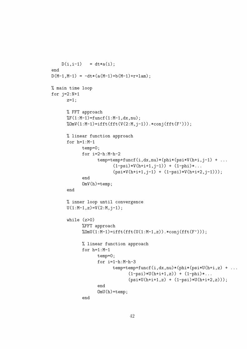
D(i,i-1) = dt*a(i);
end
D(M-1,M-1) = -dt*(a(M-1)+b(M-1)+r+lam);
% main time loop
for j=2:N+1
z=1;
% FFT approach
%F(1:M-1)=funcf(1:M-1,dx,nu);
%OmV(1:M-1)=ifft(fft(V(2:M,j-1)).*conj(fft(F’)));
% linear function approach
for h=1:M-1
temp=0;
for i=2-h:M-h-2
temp=temp+funcf(i,dx,nu)*(phi*(psi*V(h+i,j-1) + ...
(1-psi)*V(h+i+1,j-1)) + (1-phi)*...
(psi*V(h+i+1,j-1) + (1-psi)*V(h+i+2,j-1)));
end
OmV(h)=temp;
end
% inner loop until convergence
U(1:M-1,z)=V(2:M,j-1);
while (z>0)
%FFT approach
%OmU(1:M-1)=ifft(fft(U(1:M-1,z)).*conj(fft(F’)));
% linear function approach
for h=1:M-1
temp=0;
for i=1-h:M-h-3
temp=temp+funcf(i,dx,nu)*(phi*(psi*U(h+i,z) + ...
(1-psi)*U(h+i+1,z)) + (1-phi)*...
(psi*U(h+i+1,z) + (1-psi)*U(h+i+2,z)));
end
OmU(h)=temp;
end
42
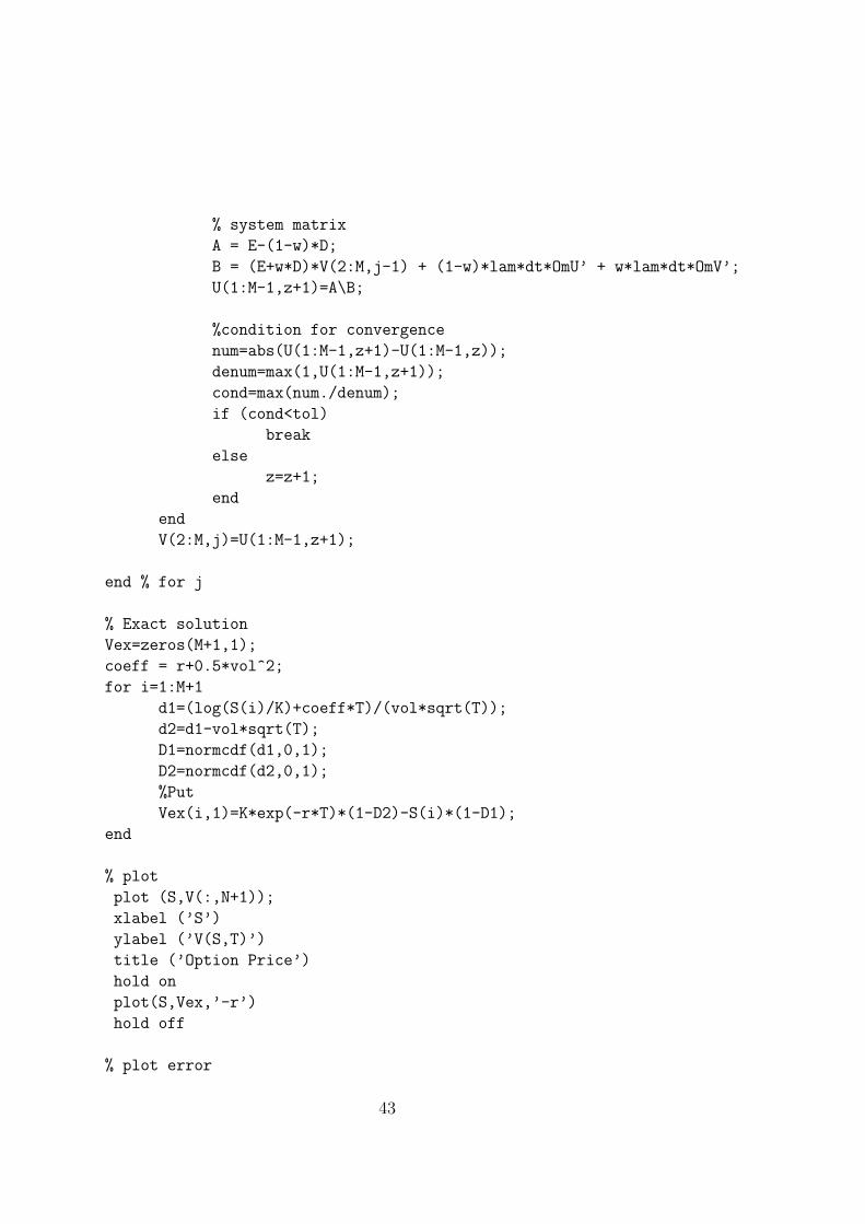
% system matrix
A = E-(1-w)*D;
B = (E+w*D)*V(2:M,j-1) + (1-w)*lam*dt*OmU’ + w*lam*dt*OmV’;
U(1:M-1,z+1)=A\B;
%condition for convergence
num=abs(U(1:M-1,z+1)-U(1:M-1,z));
denum=max(1,U(1:M-1,z+1));
cond=max(num./denum);
if (cond<tol)
break
else
z=z+1;
end
end
V(2:M,j)=U(1:M-1,z+1);
end % for j
% Exact solution
Vex=zeros(M+1,1);
coeff = r+0.5*vol^2;
for i=1:M+1
d1=(log(S(i)/K)+coeff*T)/(vol*sqrt(T));
d2=d1-vol*sqrt(T);
D1=normcdf(d1,0,1);
D2=normcdf(d2,0,1);
%Put
Vex(i,1)=K*exp(-r*T)*(1-D2)-S(i)*(1-D1);
end
% plot
plot (S,V(:,N+1));
xlabel (’S’)
ylabel (’V(S,T)’)
title (’Option Price’)
hold on
plot(S,Vex,’-r’)
hold off
% plot error
43

%plot(S,abs(Vex(:,1)-V(:,N+1)),’-g’)
%xlabel (’S’)
%ylabel (’Error value’)
%title (’Error’)
44