HAL Id: hal-01676656https://hal.archives-ouvertes.fr/hal-01676656

Submitted on 15 Feb 2018

HAL is a multi-disciplinary open accessarchive for the deposit and dissemination of sci-entific research documents, whether they are pub-lished or not. The documents may come fromteaching and research institutions in France orabroad, or from public or private research centers.

L’archive ouverte pluridisciplinaire HAL, estdestinée au dépôt et à la diffusion de documentsscientifiques de niveau recherche, publiés ou non,émanant des établissements d’enseignement et derecherche français ou étrangers, des laboratoirespublics ou privés.

Numerical stability of plasma sheathMehdi Badsi, Michel Mehrenberger, Laurent Navoret

To cite this version:Mehdi Badsi, Michel Mehrenberger, Laurent Navoret. Numerical stability of plasma sheath. 2018.<hal-01676656>

Numerical stability of plasma sheath

Mehdi Badsi1, Michel Mehrenberger2,3 and Laurent Navoret2,3

1. Institut de Mathematiques de Toulouse, UMR 5219,Universite Toulouse 3, 118 Route de Narbonne,

31400 Toulouse, France.

2. Institut de Recherche Mathematique Avancee, UMR 7501,Universite de Strasbourg et CNRS, 7 rue Rene Descartes,

67000 Strasbourg, France

3. INRIA Nancy-Grand Est, TONUS Project, Strasbourg, France

Abstract

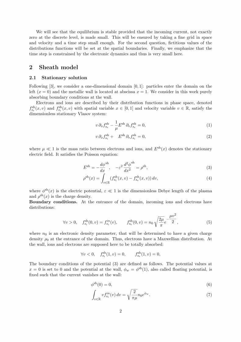
We are interested in developing a numerical method for capturing stationary sheaths,that a plasma forms in contact with a metallic wall. This work is based on a bi-species(ion/electron) Vlasov-Ampere model proposed in [3]. The main question addressed in thiswork is to know if classical numerical schemes can preserve stationary solutions with bound-ary conditions, since these solutions are not a priori conserved at the discrete level. In thecontext of high-order semi-Lagrangian method, due to their large stencil, interpolation nearthe boundary of the domain requires also a specific treatment.

1 Introduction

When a plasma is in contact with a metallic wall, stationary boundary layers, called sheaths,form. They are due to both the reflexion/absorption properties of the wall and the chargeimbalance coming from the mass difference between electrons and ions: electrons leave theplasma faster than ions. A drop of the self-consistent potential at the wall is indeed built up toaccelerate ions and decelerate electrons just as to ensure an equal flux of ions and electrons (azero current) at the wall. In this work, the starting point is a plasma sheath model proposed byBadsi et al. [3], for which a so-called kinetic Bohm criterion on the incoming ion distributionhas been found out. Numerically, the sheath potential is computed by a non-linear Poissonsolver.

We here consider the corresponding non-stationary ion/electron Vlasov-Ampere model (notethat the stability of its linearized version has been studied in [2]) and its numerical implemen-tation through a semi-Lagrangian scheme [6]. Semi-Lagrangian schemes are transport solverswith no stability conditions on the time step: time step is only constrained by the physicaldynamics that has to be captured. High-order schemes, using high degree interpolation andtime splitting, can be devised and parallel implementation can be considered. We raise here thefollowing questions:

• Question 1: How do semi-Lagrangian scheme preserve this equilibrium in time ?

• Question 2: How can we treat boundary conditions with large stencil interpolation ?

1

We will see that the equilibrium is stable provided that the incoming current, not exactlyzero at the discrete level, is made small. This will be ensured by taking a fine grid in spaceand velocity and a time step small enough. For the second question, fictitious values of thedistributions functions will be set at the spatial boundaries. Finally, we emphasize that thetime step is constrained by the electronic dynamics and thus is very small here.

2 Sheath model

2.1 Stationary solution

Following [3], we consider a one-dimensional domain [0, 1]: particles enter the domain on theleft (x = 0) and the metallic wall is located at abscissa x = 1. We consider in this work purelyabsorbing boundary conditions at the wall.

Electrons and ions are described by their distribution functions in phase space, denotedf shse (x, v) and f sh

si (x, v) with spatial variable x ∈ [0, 1] and velocity variable v ∈ R, satisfy thedimensionless stationary Vlasov system:

v ∂xfshse −

1

µEsh ∂vf

shse = 0, (1)

v ∂xfshsi + Esh ∂vf

shsi = 0, (2)

where µ � 1 is the mass ratio between electrons and ions, and Esh(x) denotes the stationaryelectric field. It satisfies the Poisson equation:

Esh = −dφdx

sh

, −ε2 d2φ

dx2

sh

= ρsh, (3)

ρsh(x) =

∫v∈R

(f shsi (x, v)− f sh

se (x, v)) dv, (4)

where φsh(x) is the electric potential, ε � 1 is the dimensionless Debye length of the plasmaand ρsh(x) is the charge density.Boundary conditions. At the entrance of the domain, incoming ions and electrons havedistributions:

∀v > 0, f shsi (0, v) = f insi (v), f sh

se (0, v) = n0

√2µ

πe−µv2

2 , (5)

where n0 is an electronic density parameter, that will be determined to have a given chargedensity ρ0 at the entrance of the domain. Thus, electrons have a Maxwellian distribution. Atthe wall, ions and electrons are supposed here to be totally absorbed:

∀v < 0, f shsi (1, v) = 0, f sh

se (1, v) = 0,

The boundary conditions of the potential (3) are defined as follows. The potential values atx = 0 is set to 0 and the potential at the wall, φw = φsh(1), also called floating potential, isfixed such that the current vanishes at the wall:

φsh(0) = 0, (6)∫v∈R

vf insi (v) dv =

√2

πµn0e

φw . (7)

2

Note that it implies that the current vanishes in the whole domain, since both electron and ionmomentum are constant in space.Solutions. Using the characteristic lines of the transport equation and under the hypothesisthat the potential is decreasing in the domain, the solution to problem (1)-(2)-(3) is given by:

f shsi (x, v) =1{

v>√−2φsh(x)

} f insi(√

v2 + 2φsh(x)), (8)

f shse (x, v) =1{

v≥−√

2µ

(φsh(x)−φsh(1))} f inse

(√v2 − 2

µφsh(x)

), (9)

where the sheath potential is the solution to the following non-linear Poisson equation:

− ε2 d2φ

dx2

sh

(x) =

[∫R+

f insi (v)v√v2 − 2φsh(x)

dv

]− 2n0√

2π

√2π eφsh(x) −

∫ +∞

√−2φw

e−v2

2 v√v2 + 2φsh(x)

dv

.(10)

complemented by the boundary conditions (6)-(7).Let consider a given charge density ρ0 ∈ R at the entrance of the domain. The problem is

solved in two steps:

1. a negative potential drop at the wall φw ≤ 0 is uniquely defined satisfying (7) providedthat the ionic distribution satisfies the relation:∫

R+f insi (v)v dv∫

R+f insi (v) dv − ρ0

≤√

2

µπ.

It satisfies the following equation:

1√µeφw

(∫v∈R

f insi (v) dv − ρ0

)+

(∫v∈R

vf insi (v) dv

)(∫ +∞

√−2φw

e−v2

2 dv

)= 0, (11)

and the associated electronic density parameter is given by:

n0 =

√π

2

∫v∈R+

f insi (v) dv − ρ0

(√

2π −∫ +∞√−2φw

e−v2

2 dv).

2. then, once this potential wall exists, the non-linear Poisson equation (10), complementedwith the boundary conditions φsh(0) = 0 and φsh(1) = φw, has a unique solution underthe kinetic Bohm criterion:∫

R+

f insi (v)

v2dv∫

R+

f insi (v) dv

<

√2π +

∫ +∞

√−2φw

e−v2/2

v2dv

√2π −

∫ +∞

√−2φw

e−v2/2 dv

.

Parameters. The equilibria has been computed by the gradient algorithm described in [3]with the following parameters:

• the dimensionless Debye length is set to ε = 0.01.

• the charge is zero at the entrance of the domain: ρ0 = 0.

3

• the incoming ion distribution is given by

f insi (v) = 1{v>0} min(1, v2/η)1√

2πσ2e−

(v−Z)2

2σ2 , η = 10−1, σ =√Ti/Te = 0.5, Z = 1.5.

(12)Z is the macroscopic ion velocity when entering the domain.

• the incoming electronic distribution is Maxwellian as given by (5). For the sake of com-pleteness, we recall the expression:

f inse (v) = 1{v>0} n0

√2µ

πe−µv2

2 , µ = 1/3672. (13)

µ is the mass ratio of a deuterium plasma.

Given these parameters, we can compute n0, φw with (11)-(1), and the sheath electric potentialφsh by solving the non-linear Poisson equation (10). In the numerical results, we take:

n0 = 0.50191266314760252, φw = −2.7839395640524267.

In practice, for future use in the non-stationary model, we store the nonlinear potential φsh ona uniform grid of N = 2048 cells, that is, at points j/N, j = 0, . . . , N .

2.2 Non-stationary model

In the non-stationary setting, electron and ion distribution functions, fse(t, x, v) and fsi(t, x, v),and the electric field, E(t, x), depend also on time t > 0. They satisfy the non-linear Vlasov-Ampere system:

∂tfse + v ∂xfse −1

µE ∂vfse = 0, (14)

∂tfsi + v ∂xfsi + E ∂vfsi = 0, (15)

ε2 ∂tE = −J, (16)

where J denotes the current density:

J(t, x) =

∫v∈R

v (fsi(t, x, v)− fse(t, x, v)) dv.

Initial data. The initial data are given by the stationary solution:

fse(0, x, v) = f shse (x, v), fsi(0, x, v) = f sh

si (x, v), E(0, x) = Esh(x).

We note that the initial electric field E(x, 0) satisfies the following Poisson equation:

ε2∂xE(0, x) = nsi(0, x)− nse(0, x), (17)∫ 1

0E(t, x) dx = −φw, (18)

where the densities nsi and nse are given by:

nse(t, x) =

∫v∈R

fse(t, x, v) dv, nsi(t, x) =

∫v∈R

fsi(x, v) dv,

and φw is the floating potential at x = 1.

4

3 Numerical scheme

We solve system (14)-(15)-(16) using a semi-Lagrangian scheme. Due to the large mass ratiobetween electrons and ions, the computational domain of electrons will be larger than the ionone and thus velocity meshes have to be different for the two kinds of particles.Mesh notations. We consider uniform cartesian meshes for both spatial domain [0, 1] andvelocity domain [vmin, vmax]. Considering Nx+1 points in the spatial direction and Nv+1 pointsin the velocity one, mesh points are denoted (xi, vj) = (i∆x, vmin + j∆v) for all 0 ≤ i ≤ Nx and0 ≤ j ≤ Nv with ∆x = 1/Nx and ∆v = (vmax − vmin)/Nv. Note that the definitions relativeto the velocity domain implicitly depend on the particle s ∈ {se, si} under consideration. Wedenote by fns,(i,j) the approximate value of the distribution function fs at point (xi, vj) at timetn = n∆t, with ∆t > 0 and n ∈ N, and Eni the approximate value of the electric field at pointxi.

3.1 Initialization of the electric field

The solution to system (17)-(18) is given by:

E(x) =

∫ x

0

nsi(y)− nse(y)

ε2dy − φw −

∫ 1

0

∫ x

0

nsi(y)− nse(y)

ε2dydx. (19)

The charge densities ns, s ∈ {se, si} are computed at grid points xi using the trapezoidal formulain the velocity direction from the distributions functions 1. We then consider a reconstructionat any point x = xi + α∆x ∈ [0, 1], with α ∈ [0, 1], by local centered Lagrange interpolation ofdegree 2d+ 1 with d ∈ N:

ns,h(x) =d+1∑k=−d

ns,i+k Lk(α),

where Lk are the elementary Lagrange polynomials:

Lk(α) =

d+1∏i=−di 6=k

(α− i)/(k − i). (20)

Note that the densities have to be defined at points outside of the domain when d > 0. This willbe done by expanding the definition of the distribution functions. This point will be detailed inSection 3.3. The discrete electric field at grid points xi is then obtained from (19) in which nsare replaced by their discrete counterparts ns,h. The involved integrals are computed exactlyand the overall scheme has O(∆x2d+2) accuracy.

3.2 Splitting

To solve the Vlasov-Ampere system, we use a splitting between space and velocity dynamicsand write it as a succession of one-dimensional advections. More precisely, we consider thefollowing dynamics: the kinetic transport system given by:

(T ) ∂tfse + v ∂xfse = 0, (21)

∂tfsi + v ∂xfsi = 0, (22)

ε2 ∂tE = −J, (23)

1The trapezoidal formula is spectrally accurate for smooth periodic data and remains accurate when thevelocity domain is large enough so that the distribution equals zero at the boundaries (up to machine precision)and can be considered as periodic. We yet point out that the electron distribution (9) has a discontinuity invelocity, which deteriorates the accuracy.

5

and the electric transport system, given by:

(U) ∂tfse −1

µE ∂vfse = 0, (24)

∂tfsi + E ∂vfsi = 0, (25)

ε2 ∂tE = 0. (26)

Since the electric field is constant in time in this second step, both dynamics T and U areadvections at constant velocities. In practice, to obtain second order accuracy in time, weconsider the Strang splitting which consists in computing for s ∈ {se, si}{(

fn+1s,(i,j)

)i,j, (En+1

i )i

}=[Uh,∆t/2 ◦ Th,∆t ◦ Uh,∆t/2

]{(fns,(i,j))i,j , (E

ni )i

}where Th,τ and Uh,τ are discrete approximations of T and U over a time interval τ .

Each transport equation is solved using a semi-Lagrangian scheme with centered Lagrangeinterpolation of degree 2d + 1. We thus consider the discretized version of the kinetic andelectric transport dynamics. Operator Th,τ : ((fs,(i,j)), (Ei)i)→ ((f∗s,(i,j)), (E

∗i )i) consists in the

following: for any grid points (xi, vj), we define the shifted index i∗ and α ∈ [0, 1] such thatxi − vjτ = xi∗ + α∆x and then the distribution function is given by:

f∗s,(i,j) =d+1∑k=−d

fs,(i∗+k,j)Lk(α),

where the (Lk) are defined in (20), and the electric field at point xi is given by:

E∗i = Ei − τJi + J∗i

2,

where the current density (Ji)i (resp. (J∗i )i) is computed by trapezoidal rule in velocity from thediscrete distribution function (fi,j) (resp. (f∗i,j)). We thus exactly solve in time the transportequations (21)-(22) at the grid points, starting from the interpolated distribution function inthe spatial direction, while the Ampere equation (23) is computed using a second order Crank-Nicolson scheme. The interpolation requires values of the distribution function outside thedomain: we explain in the next section how to extrapolate it.

Operator Uh,τ : ((fs,(i,j)), (Ei)i) → ((f∗s,(i,j)), (E∗i )i) consists in the following: for any grid

points (xi, vj), we define the shifted indexes j∗si , j∗se and αsi , αse ∈ [0, 1] such that vj − Eiτ =

vj∗si+ αsi∆vsi and vj + 1

µEiτ = vj∗se + αse∆vse and then

f∗s,(i,j) =d+1∑k=−d

fs,(i,j∗s+k)Lk(αs),

E∗i = Ei.

For this advection in velocity Uh,τ , periodic boundary conditions are used; we have here madethe presentation for Lagrange interpolation, as it is used for advection in space, but otheradvection scheme can be used; in particular, in the numerical results, we will use cubic splines.

3.3 Boundary conditions

In both the initial computation of the electric field and the advection in space Th,τ , the pro-posed numerical scheme requires to take values of the distribution function outside the physicaldomain.

6

For any xi = i∆x < 0 and vj , we consider the following extrapolation at the entry x = 0:

fs,(i,j) =

{fs(0, 0, vj), if vj ≥ 0,

2fs,(0,j) − fs,(−i,j), if vj < 0.

For any xi+Nx = (i + Nx)∆x > 1 and vj , we consider the following extrapolation at the wallx = 1:

fs,(i+Nx,j) =

{2fs,(Nx,j) − fs,(Nx−i,j) if vj ≥ 0,

0 if vj < 0.

This corresponds to a purely Dirichlet condition for incoming velocities and an extension byimparity for leaving velocities (also called butterfly procedure).

4 Numerical results

4.1 Sheath test-case

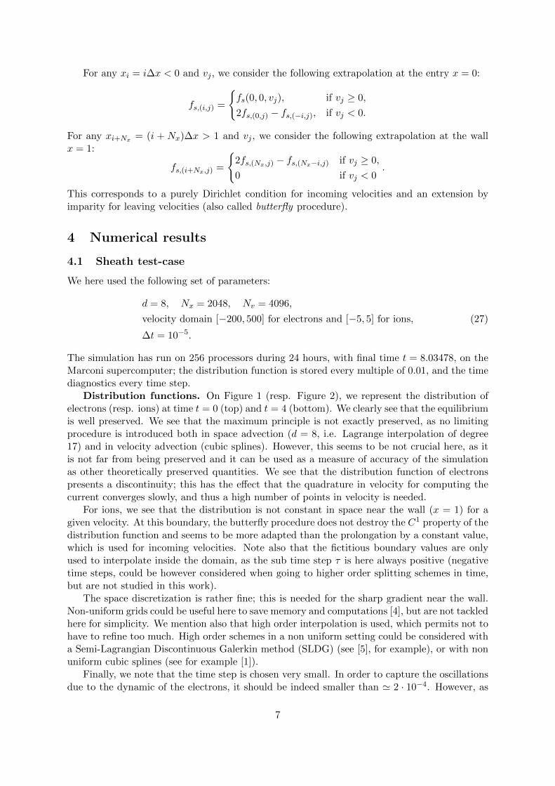
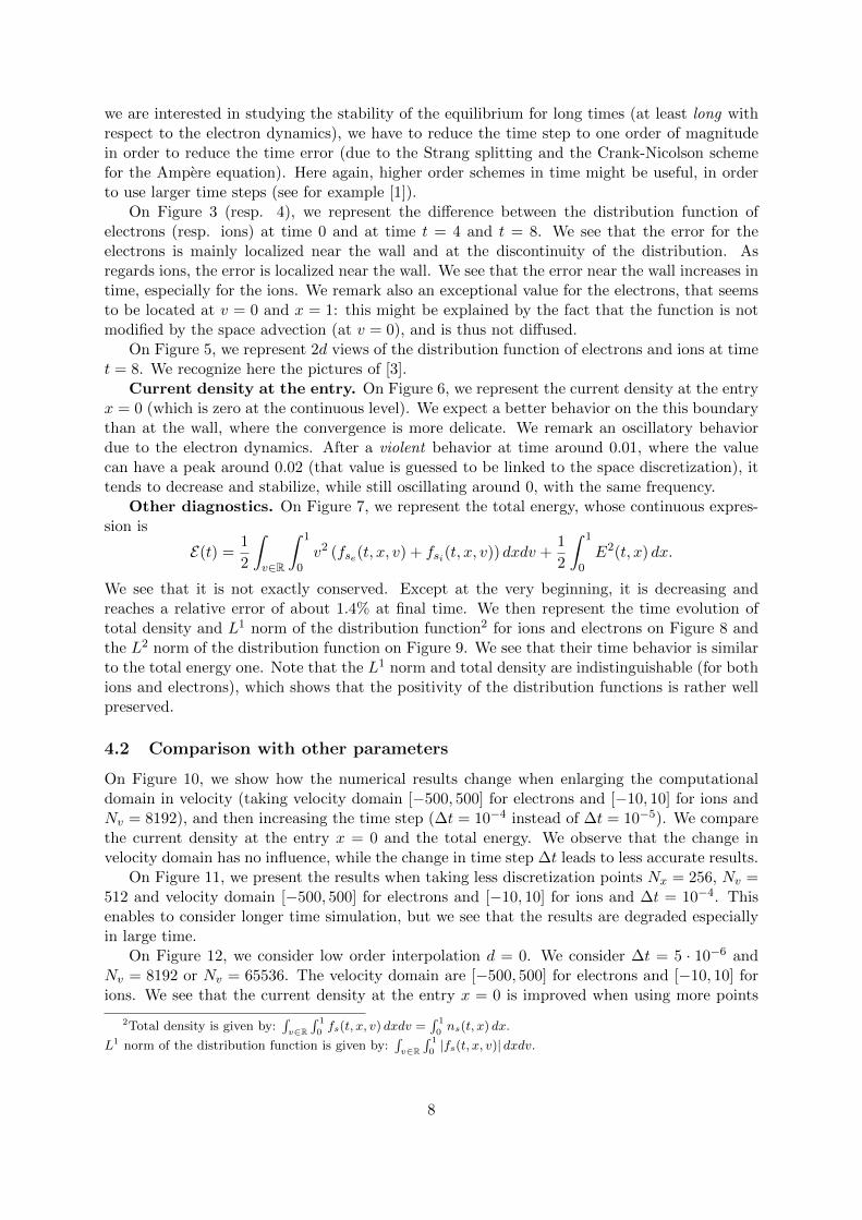
We here used the following set of parameters:

d = 8, Nx = 2048, Nv = 4096,

velocity domain [−200, 500] for electrons and [−5, 5] for ions, (27)

∆t = 10−5.

The simulation has run on 256 processors during 24 hours, with final time t = 8.03478, on theMarconi supercomputer; the distribution function is stored every multiple of 0.01, and the timediagnostics every time step.

Distribution functions. On Figure 1 (resp. Figure 2), we represent the distribution ofelectrons (resp. ions) at time t = 0 (top) and t = 4 (bottom). We clearly see that the equilibriumis well preserved. We see that the maximum principle is not exactly preserved, as no limitingprocedure is introduced both in space advection (d = 8, i.e. Lagrange interpolation of degree17) and in velocity advection (cubic splines). However, this seems to be not crucial here, as itis not far from being preserved and it can be used as a measure of accuracy of the simulationas other theoretically preserved quantities. We see that the distribution function of electronspresents a discontinuity; this has the effect that the quadrature in velocity for computing thecurrent converges slowly, and thus a high number of points in velocity is needed.

For ions, we see that the distribution is not constant in space near the wall (x = 1) for agiven velocity. At this boundary, the butterfly procedure does not destroy the C1 property of thedistribution function and seems to be more adapted than the prolongation by a constant value,which is used for incoming velocities. Note also that the fictitious boundary values are onlyused to interpolate inside the domain, as the sub time step τ is here always positive (negativetime steps, could be however considered when going to higher order splitting schemes in time,but are not studied in this work).

The space discretization is rather fine; this is needed for the sharp gradient near the wall.Non-uniform grids could be useful here to save memory and computations [4], but are not tackledhere for simplicity. We mention also that high order interpolation is used, which permits not tohave to refine too much. High order schemes in a non uniform setting could be considered witha Semi-Lagrangian Discontinuous Galerkin method (SLDG) (see [5], for example), or with nonuniform cubic splines (see for example [1]).

Finally, we note that the time step is chosen very small. In order to capture the oscillationsdue to the dynamic of the electrons, it should be indeed smaller than ' 2 · 10−4. However, as

7

we are interested in studying the stability of the equilibrium for long times (at least long withrespect to the electron dynamics), we have to reduce the time step to one order of magnitudein order to reduce the time error (due to the Strang splitting and the Crank-Nicolson schemefor the Ampere equation). Here again, higher order schemes in time might be useful, in orderto use larger time steps (see for example [1]).

On Figure 3 (resp. 4), we represent the difference between the distribution function ofelectrons (resp. ions) at time 0 and at time t = 4 and t = 8. We see that the error for theelectrons is mainly localized near the wall and at the discontinuity of the distribution. Asregards ions, the error is localized near the wall. We see that the error near the wall increases intime, especially for the ions. We remark also an exceptional value for the electrons, that seemsto be located at v = 0 and x = 1: this might be explained by the fact that the function is notmodified by the space advection (at v = 0), and is thus not diffused.

On Figure 5, we represent 2d views of the distribution function of electrons and ions at timet = 8. We recognize here the pictures of [3].

Current density at the entry. On Figure 6, we represent the current density at the entryx = 0 (which is zero at the continuous level). We expect a better behavior on the this boundarythan at the wall, where the convergence is more delicate. We remark an oscillatory behaviordue to the electron dynamics. After a violent behavior at time around 0.01, where the valuecan have a peak around 0.02 (that value is guessed to be linked to the space discretization), ittends to decrease and stabilize, while still oscillating around 0, with the same frequency.

Other diagnostics. On Figure 7, we represent the total energy, whose continuous expres-sion is

E(t) =1

2

∫v∈R

∫ 1

0v2 (fse(t, x, v) + fsi(t, x, v)) dxdv +

1

2

∫ 1

0E2(t, x) dx.

We see that it is not exactly conserved. Except at the very beginning, it is decreasing andreaches a relative error of about 1.4% at final time. We then represent the time evolution oftotal density and L1 norm of the distribution function2 for ions and electrons on Figure 8 andthe L2 norm of the distribution function on Figure 9. We see that their time behavior is similarto the total energy one. Note that the L1 norm and total density are indistinguishable (for bothions and electrons), which shows that the positivity of the distribution functions is rather wellpreserved.

4.2 Comparison with other parameters

On Figure 10, we show how the numerical results change when enlarging the computationaldomain in velocity (taking velocity domain [−500, 500] for electrons and [−10, 10] for ions andNv = 8192), and then increasing the time step (∆t = 10−4 instead of ∆t = 10−5). We comparethe current density at the entry x = 0 and the total energy. We observe that the change invelocity domain has no influence, while the change in time step ∆t leads to less accurate results.

On Figure 11, we present the results when taking less discretization points Nx = 256, Nv =512 and velocity domain [−500, 500] for electrons and [−10, 10] for ions and ∆t = 10−4. Thisenables to consider longer time simulation, but we see that the results are degraded especiallyin large time.

On Figure 12, we consider low order interpolation d = 0. We consider ∆t = 5 · 10−6 andNv = 8192 or Nv = 65536. The velocity domain are [−500, 500] for electrons and [−10, 10] forions. We see that the current density at the entry x = 0 is improved when using more points

2Total density is given by:∫v∈R

∫ 1

0fs(t, x, v) dxdv =

∫ 1

0ns(t, x) dx.

L1 norm of the distribution function is given by:∫v∈R

∫ 1

0|fs(t, x, v)| dxdv.

8

Figure 1: Distribution function of electrons at time t = 0 (top) and t = 4 (bottom); X standsfor x, Y for v and Z for f(t, x, v). Parameters given in (27).

9

Figure 2: Distribution function of ions at time t = 0 (top) and t = 4 (bottom); X stands for x,Y for v and Z for f(t, x, v). Parameters given in (27).

10

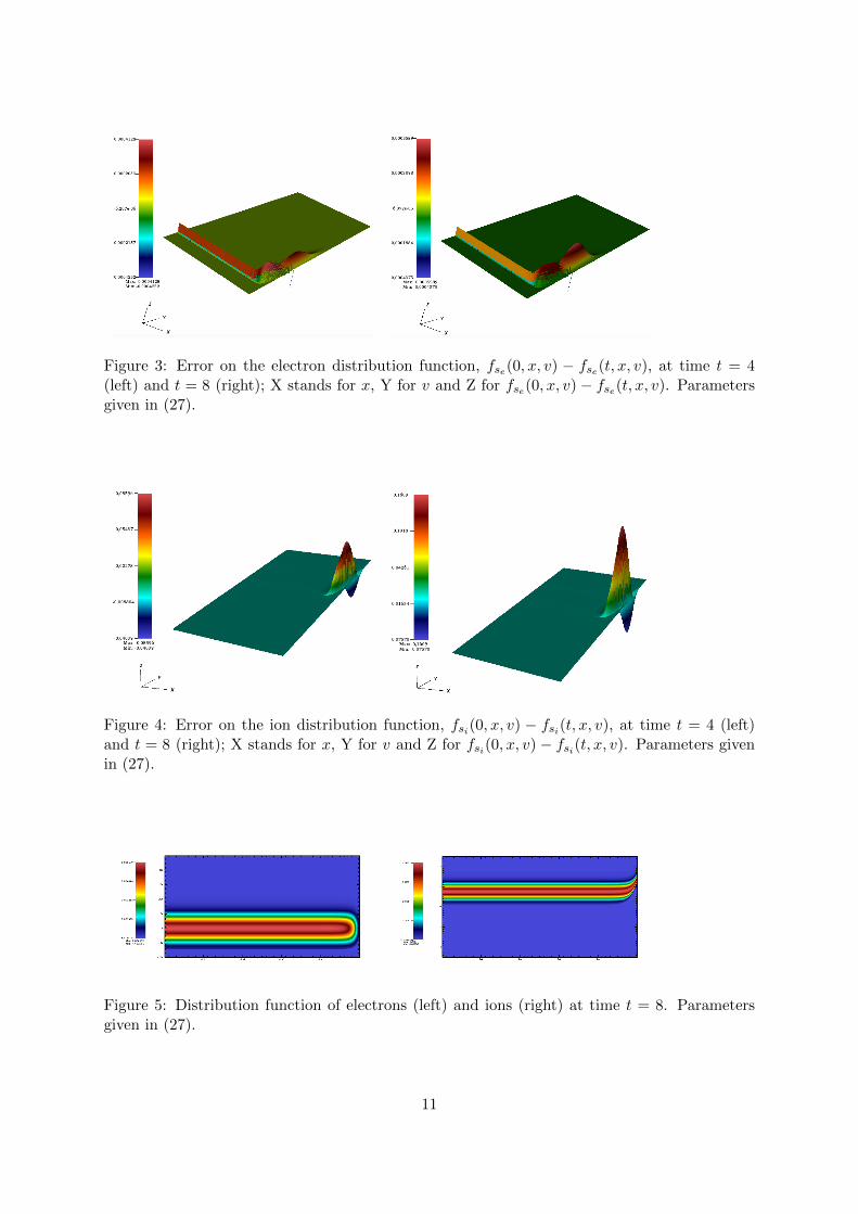
Figure 3: Error on the electron distribution function, fse(0, x, v) − fse(t, x, v), at time t = 4(left) and t = 8 (right); X stands for x, Y for v and Z for fse(0, x, v)− fse(t, x, v). Parametersgiven in (27).

Figure 4: Error on the ion distribution function, fsi(0, x, v) − fsi(t, x, v), at time t = 4 (left)and t = 8 (right); X stands for x, Y for v and Z for fsi(0, x, v)− fsi(t, x, v). Parameters givenin (27).

Figure 5: Distribution function of electrons (left) and ions (right) at time t = 8. Parametersgiven in (27).

11

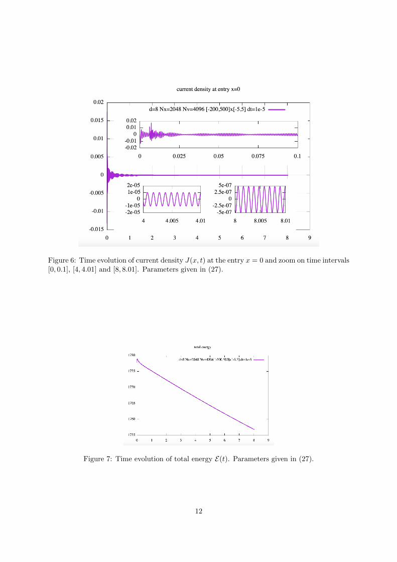
Figure 6: Time evolution of current density J(x, t) at the entry x = 0 and zoom on time intervals[0, 0.1], [4, 4.01] and [8, 8.01]. Parameters given in (27).

Figure 7: Time evolution of total energy E(t). Parameters given in (27).

12

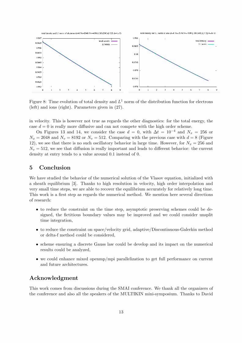
Figure 8: Time evolution of total density and L1 norm of the distribution function for electrons(left) and ions (right). Parameters given in (27).

in velocity. This is however not true as regards the other diagnostics: for the total energy, thecase d = 0 is really more diffusive and can not compete with the high order scheme.

On Figures 13 and 14, we consider the case d = 0, with ∆t = 10−4 and Nx = 256 orNx = 2048 and Nv = 8192 or Nv = 512. Comparing with the previous case with d = 8 (Figure12), we see that there is no such oscillatory behavior in large time. However, for Nx = 256 andNv = 512, we see that diffusion is really important and leads to different behavior: the currentdensity at entry tends to a value around 0.1 instead of 0.

5 Conclusion

We have studied the behavior of the numerical solution of the Vlasov equation, initialized witha sheath equilibrium [3]. Thanks to high resolution in velocity, high order interpolation andvery small time steps, we are able to recover the equilibrium accurately for relatively long time.This work is a first step as regards the numerical method. We mention here several directionsof research:

• to reduce the constraint on the time step, asymptotic preserving schemes could be de-signed, the fictitious boundary values may be improved and we could consider unsplittime integration,

• to reduce the constraint on space/velocity grid, adaptive/Discontinuous-Galerkin methodor delta-f method could be considered,

• scheme ensuring a discrete Gauss law could be develop and its impact on the numericalresults could be analyzed,

• we could enhance mixed openmp/mpi parallelization to get full performance on currentand future architectures.

Acknowledgment

This work comes from discussions during the SMAI conference. We thank all the organizers ofthe conference and also all the speakers of the MULTIKIN mini-symposium. Thanks to David

13

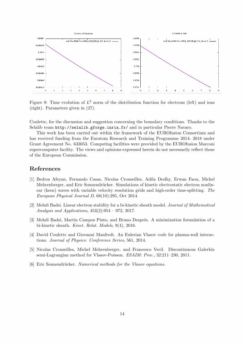
Figure 9: Time evolution of L2 norm of the distribution function for electrons (left) and ions(right). Parameters given in (27).

Coulette, for the discussion and suggestion concerning the boundary conditions. Thanks to theSelalib team http://selalib.gforge.inria.fr/ and in particular Pierre Navaro.

This work has been carried out within the framework of the EUROfusion Consortium andhas received funding from the Euratom Research and Training Programme 2014- 2018 underGrant Agreement No. 633053. Computing facilities were provided by the EUROfusion Marconisupercomputer facility. The views and opinions expressed herein do not necessarily reflect thoseof the European Commission.

References

[1] Bedros Afeyan, Fernando Casas, Nicolas Crouseilles, Adila Dodhy, Erwan Faou, MichelMehrenberger, and Eric Sonnendrucker. Simulations of kinetic electrostatic electron nonlin-ear (keen) waves with variable velocity resolution grids and high-order time-splitting. TheEuropean Physical Journal D, 68(10):295, Oct 2014.

[2] Mehdi Badsi. Linear electron stability for a bi-kinetic sheath model. Journal of MathematicalAnalysis and Applications, 453(2):954 – 972, 2017.

[3] Mehdi Badsi, Martin Campos Pinto, and Bruno Despres. A minimization formulation of abi-kinetic sheath. Kinet. Relat. Models, 9(4), 2016.

[4] David Coulette and Giovanni Manfredi. An Eulerian Vlasov code for plasma-wall interac-tions. Journal of Physics: Conference Series, 561, 2014.

[5] Nicolas Crouseilles, Michel Mehrenberger, and Francesco Vecil. Discontinuous Galerkinsemi-Lagrangian method for Vlasov-Poisson. ESAIM: Proc., 32:211–230, 2011.

[6] Eric Sonnendrucker. Numerical methods for the Vlasov equations.

14

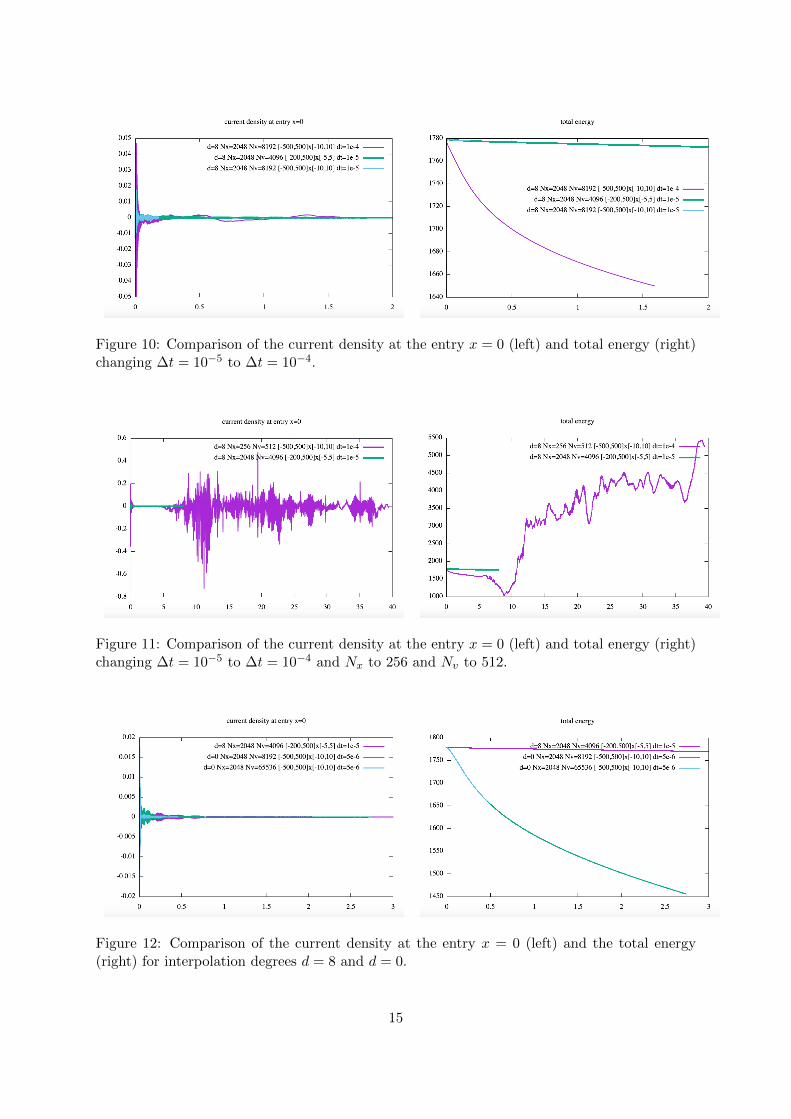
Figure 10: Comparison of the current density at the entry x = 0 (left) and total energy (right)changing ∆t = 10−5 to ∆t = 10−4.

Figure 11: Comparison of the current density at the entry x = 0 (left) and total energy (right)changing ∆t = 10−5 to ∆t = 10−4 and Nx to 256 and Nv to 512.

Figure 12: Comparison of the current density at the entry x = 0 (left) and the total energy(right) for interpolation degrees d = 8 and d = 0.

15

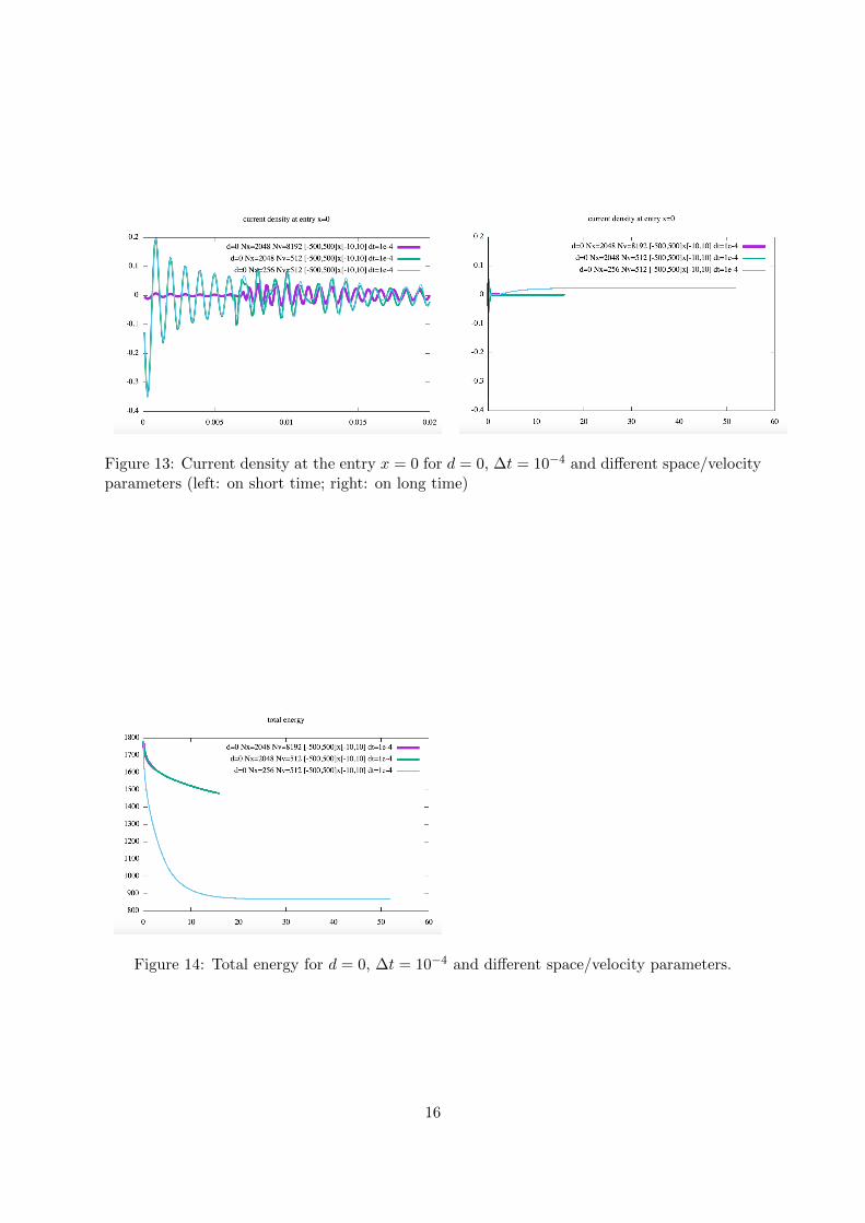
Figure 13: Current density at the entry x = 0 for d = 0, ∆t = 10−4 and different space/velocityparameters (left: on short time; right: on long time)

Figure 14: Total energy for d = 0, ∆t = 10−4 and different space/velocity parameters.

16