Embed Size (px)
Citation preview

VALUATION AND PRICING OF EQUITY SECURITIES IN AN EMERGING STOCK MARKET: EVIDENCE FROM THE NIGERIAN BANKING SECTOR
A THESIS SUBMITTED TO THE DEPARTMENT OF
FACULTY OF
1
NWUDE CHUKE EMMANUEL PG/Ph.D/2000/31748
VALUATION AND PRICING OF EQUITY SECURITIES IN AN EMERGING STOCK MARKET: EVIDENCE FROM THE NIGERIAN BANKING SECTOR
Business Administration
A THESIS SUBMITTED TO THE DEPARTMENT OF BANKING AND FINANCE
FACULTY OF BUSINESS ADMINISTRATION, UNIVERSITY OF NIGERIA ENUGU
CAMPUS
Webmaster Digitally Signed by Webmaster’s Name DN : CN = Webmaster’s name O= University of Nigeria, NsukkaOU = Innovation Centre
2010
UNIVERSITY OF NIGERIA
VALUATION AND PRICING OF EQUITY SECURITIES IN AN EMERGING STOCK MARKET: EVIDENCE FROM THE NIGERIAN BANKING SECTOR
BANKING AND FINANCE,
, UNIVERSITY OF NIGERIA ENUGU
DN : CN = Webmaster’s name O= University of Nigeria, Nsukka
UNIVERSITY OF NIGERIA
2
VALUATION AND PRICING OF EQUITY SECURITIES IN AN EMERGING STOCK MARKET: EVIDENCE FROM THE NIGERIAN BANKING SECTOR
BY NWUDE CHUKE EMMANUEL
PG/Ph.D/2000/31748
DEPARTMENT OF BANKING AND FINANCE FACULTY OF BUSINESS ADMINISTRATION
UNIVERSITY OF NIGERIA NSUKKA ENUGU CAMPUS
APRIL 2010
3
VALUATION AND PRICING OF EQUITY SECURITIES IN AN EMERGING STOCK MARKET: EVIDENCE FROM THE NIGERIAN BANKING SECTOR
BY NWUDE CHUKE EMMANUEL PG/Ph.D/2000/31748 A thesis submitted to the Department of Banking and Finance, Faculty of Business Administration, University of Nigeria Enugu campus, in fulfilment of the requirements for the award of a Doctor of Philosophy(Ph.D) Degree in Finance DEPARTMENT OF BANKING AND FINANCE FACULTY OF BUSINESS ADMINISTRATION UNIVERSITY OF NIGERIA ENUGU CAMPUS SUPERVISOR: PROF. C. U. UCHE APRIL 2010
4
APPROVAL
Nwude Chuke Emmanuel, a postgraduate student in the Department of Banking and Finance,
Faculty of Business Administration, University of Nigeria, Enugu campus, with registration
number PG/Ph.D/2000/31748 has satisfactorily completed the requirements for the award of
Doctor of Philosophy in Finance.
This thesis has been approved for the Department of Banking and Finance, Faculty of
Business Administration, University of Nigeria, Enugu Campus.
BY
Professor C. U. Uche Mrs N. J. Modebe Supervisor Head of Department
Professor S. I. Owualah Dr U. J. F. Ewurum External Examiner Internal Examiner

5
CERTIFICATION I, Nwude Chuke Emmanuel, a postgraduate student in the Department of Banking and Finance, Faculty of Business Administration, University of Nigeria, Enugu campus, with registration number PG/Ph.D/2000/31748 carried out this research work on “Valuation and Pricing of Equity Securities in an Emerging Stock Market: Evidence from the Nigerian Banking Sector” in fulfilment of the requirements for the award of Doctor of Philosophy in Finance. The work embodied in this thesis is original and has not been submitted in part or full for any
other Diploma or Degree of this or any other University.
Chuke E. Nwude Student

6
DEDICATION
This research is dedicated to Almighty God, the Fountain of knowledge, my Cornerstone, my
Creator, my Protector, my Shield, the Solid Rock on which I stand and the Everlasting God
whose gifts are irrevocable. He has shown Himself strong in my life, as He does for all whose
hearts are perfect towards Him. To you God alone is all the glory.

7
ACKNOWLEDGEMENTS First, I give glory and praise to God for His enabling grace that made it possible for me to
complete this work despite all odds. I am sincerely grateful to my supervisors, Professor
Chibuike Ugochukwu Uche and Dr A. M. O. Anyafo (of blessed memory) for their
contributions without which this work would not have been a success. I would like to thank
Professor Chibuike Ugochukwu Uche in a special way, for incisively inspiring research in
this direction and for his invaluable suggestions in the course of this work. His sacrifices
ensured and insured the completion of this work. In the same vein, I express my profound
gratitude to our erudite first professor of finance University of Nigeria Nsukka ever produced,
in the person of Professor F. O. Okafor, for his incalculable sacrifice to ensure continuity in
academic excellence in the Department in particular and the Faculty of Business
Administration in general, for his understanding, assistance and moral support in all my
academic endeavours.
Equally worthy of mention are Prof Ikechukwu Nwosu, Professor (Mrs) D. Nnoli, Dr U. J. F.
Ewurum, Dr (Mrs) Eby Ogamba, Dr J.U.J Onwumere, Dr (Mrs) Justie Nnabuko, Dr I. C. O.
Nwaizugbo who normally called to know what was holding me from completing my work,
which they know I have the capacity. I am particularly appreciative of your interests that
urged me on to complete this work.
My thanks go to Professor David Webb of London School of Economics and Political
Science, Professor Olaseni Akintola-Bello of Arbitrage Consulting Group Lagos, Professor
W. I. C. Iyiegbuniwe and HRH Professor Sunday Owualah both of Department of Banking
and Finance, University of Lagos, for their invaluable contributions in this work.
I also wish to express my profound gratitude to the Dean, Faculty of Business
Administration, Professor Uche Modum, and the Head, Department of Banking and Finance,
Mrs Nwanne J. Modebe, for their understanding, assistance and moral support.
Finally, I wish to acknowledge the support of my dear God-sent wife Comie, and children,
KC, Somtie, Chisom, Dinma-baby, for their prayers, patience and understanding for the time
I had to stay away from their cherished company to see to the tidying up of this work.

8
ABSTRACT In finance, there is widespread agreement that the Capital Asset Pricing Model (CAPM) and Whitbeck-Kisor Model (WKM) are good predictors of share price movements in stock markets. While the above assertion had been empirically validated in several stock markets in developed economies, there have been few such studies in the stock markets of developing economies like Nigeria. Such studies have now become imperative given the recent developments that have seen the Nigerian stock market capitalization increasing from N276, 111,743,197.30 on January 2, 1998 to N10, 180,292,984,225.00 on December 31, 2007 without a relative increase in the volume of stocks being traded. To this effect, the major objective of this study is to examine the relevance of some of the established models that guide stock price movements in the Nigerian context. For this study, particular reference is placed on the banking sector, which dominates other sectors in terms of market capitalization and volume traded in the Nigerian Stock Exchange market. Data for this research were collected mainly from secondary sources such as audited annual reports of sampled banks, periodicals, various publications of Central Bank of Nigeria such as annual reports and statistical bulletins, Daily official lists and statistical year books of Nigerian Stock Exchange, different publications of Securities and Exchange Commission and Nigerian Deposit Insurance Corporation. The data set for the study consists of all the 23 pre-consolidation and 20 out of the 21 post-consolidation bank equity stocks quoted on the Nigerian Stock Exchange. Spring bank was not included because it has not published any financial statements after the bank consolidation exercise. The study covered an eight year period (2000-2007), pre and post bank consolidation periods. Three hypotheses were tested using the Capital Asset Pricing Model (CAPM) and Whitbeck-Kisor Model (WKM), multiple linear regression model, and Pearson product moment correlation coefficient. The findings of the study show that the application of the Capital Asset Pricing Model(CAPM) to Nigerian banking sector data indicate that 100 percent of the banking stocks were either undervalued or overvalued while zero percent were correctly valued. The application of the Whitbeck-Kisor Model (WKM) to Nigerian banking sector data shows that 4.4 percent of the banking stocks were correctly valued while the remaining 95.6 percent were either undervalued or overvalued. Hence none of the tested models guided the valuation and pricing of equity securities in the Nigerian Stock Exchange market from 2000-2007. There was no statistically significant relationship between the price-earnings ratio and the level of earnings growth, dividend payout ratio, and the variability of earnings of the sampled stocks in the Nigerian Stock Exchange market from 2000-2007.

9
TABLE OF CONTENTS Title fly i Title Page ii Approval iii Certification iv Dedication v Acknowledgements vi Abstract vii Table of contents viii CHAPTER ONE: INTRODUCTION
1.1 Background of Study 1 1.2 Statement of Problem 9 1.3 Objectives of Study 10 1.4 Research Questions 11 1.5 Statements of Research Hypotheses 11 1.6 Scope of Study 11 1.7 Significance of Study 12 1.8 Limitations of the Study 14 References 15 CHAPTER TWO: REVIEW OF RELATED LITERATURE 2.1Theoretical Concepts 19 2.1.1The Concept of Value 19 2.1.2 Approaches to common stocks valuation 22 2.1.2.1 The Discounted cash Flow (DCF) Valuation 22 2.1.2.2 Dividend Discount Model (DDM) 24 2.1.2.3 Free Cash Flow Discount Model (FCFDM) 27 2.1.2.4 Relative Valuation Approach 29 2.1.2.5 Earnings Multiplier (P/E ratio) Model 29 2.1.2.6 Price/Earnings to Growth Rate ratio (PEG) 30 2.1.2.7 Price/Book Value (PBV) 31 2.1.2.8 Price/Sales ratio (PSR) 31
2.1.2.9 Price/Cash Flow Multiple 31
2.1.2.10 Enterprise Value to Sales (EVS) ratio 31
2.1.2.11 EV/EBITDA (EVE) ratio 32
2.1.2.12 Subscription-member-based Valuation 32
2.1.2.13 Models for setting the offer price 32
2.1.2.14 Dividend based Value 32
2.1.2.15 Net Asset based Value 33
2.1.2.16 Relative Value 33
2.1.2.17 Net Book Value of Asset per share 33
2.1.2.18 Current Cost of Asset per share 34
2.1.2.19 Number of Years Purchase of Earnings 34
2.1.2.20 Price/Earnings Multiplier 34
10
2.1.2.21 Liquidation Value 35
2.1.2.22 Replacement Value 35
2.1.2.23 Stock price relative to Treasury bonds 35
2.1.2.24 Stock price relative to equity value per share 35
2.1.2.25 With Constant Growth Dividend Trend to Perpetuity 36
2.1.2.26 Using variable Dividend Model (for a definite period) 38
2.1.2.27 Non-Growth, Non-plough back, Constant Dividend 38
2.1.3 Sentiments that Affect Stock Value 39
2.1.3.1 Investors Preferences 39
2.1.3.2 Fundamental Analysis 40
2.1.3.3 Technical Analysis 40
2.1.3.4 Random Walk Hypothesis 40
2.1.3.5 Noise Trading 41
2.1.3.6 The Efficient Market Hypothesis 41
2.2 Survey of Related Studies 42
2.2.0 Earnings Models 47
2.2.1 Certainty Equivalent Models 48
2.2.2 Excess Return Models 49
2.2.3 Measuring Economic Value Added 50
2.2.4 Variants of Economic Value Added 50
2.2.5 Adjusted Present Value (APV) Models 51
2.2.6 Variants of APV 53
2.2.7 Asset Based Valuation 53
2.2.8 Accounting Valuations 53
2.2.8.1 Book Value Based Valuation 53
2.2.8.2 Book Value plus Earnings Valuation Model 54
2.2.8.3 Fair Value Accounting 55
2.2.8.4 Liquidation Valuation 55
2.2.9 Relative Valuation 56
2.2.10 Determinants of Multiples 58
2.2.11 Comparable Firms 60
2.2.12 Valuation Based on P/E ratio: Determination of P/E ratio 63
2.2.13 Sector regressions 65
2.2.14 Market Regression 66

11
2.2.15 Estimation of Fundamentals 66
2.2.15.1 Estimation of beta coefficient 66
2.2.15.2 The CAPM 68
2.3 Conclusion 70
References 72
CHAPTER THREE: RESEARCH METHODOLOGY
3.0 Introduction 82 3.1Theoretical framework for the Study 82 3.2 Research Design 83 3.3 Nature and Sources of Data 84 3.4 Population and Sample 84 3.5 Valuation Methodology 85 3.6 Model specifications 86 3.6.1 Application of CAPM to Nigerian banking Industry Data 86 3.6.1.1 Estimating the Expected Rate of Return 86 3.6.1.2 Estimating the Risk-free Rate 86 3.6.1.3 Estimating the Beta Coefficient 87 3.6.1.4 Estimating the Market Return 87 3.6.1.5 Estimating the Actual Rates of Return of an Asset 88 3.6.1.6 Geometric Mean 89 3.6.1.7 Assessment of Level of Variation 90 3.6.2 Application of KWM to Nigerian Banking Industry Data 90 3.6.2.1 Estimating Normal P/E ratio 90 3.7 Summary 91 References 94 CHAPTER FOUR: DATA PRESENTATION AND ANALYSIS 4.0 Introduction 96 4.1 Data Presentation 96 4.2 Data Analysis 101 4.3 Test of Hypotheses 114 CHAPTER FIVE: SUMMARY OF FINDINGS, CONCLUSIONS AND RECOMMENDATIONS 5.0 Introduction 118 5.1 Summary of Findings 118 5.2 Conclusions 126 5.3 Recommendations 128 Appendix 130 Bibliography 186
12
CHAPTER ONE
INTRODUCTION
1.1 BACKGROUND OF STUDY
Research is an organized enquiry or investigation into any subject or area of interest with the
aim of providing information for solving identified problem(s). It can be a revision of
accepted theories or laws in the light of new facts or practical application of such new or
revised theories or laws. It can also be a collection of information about a particular subject.
Research is all about facts and logic. A research interest can come up from various sources
such as contemporary events, areas of further research as indicated in past researched works,
comments in journal articles, discussions, and assertions that are subject to validation.
Research interest can also be sparked off by phenomena characterized by controversy and
need investigation to find out more.
In finance, there is widespread agreement that the Capital Asset Pricing Model (CAPM) and
Whitbeck-Kisor Model (WKM) are good predictors of share price movements in stock
markets. While the above assertion had been empirically validated in several stock markets in
developed economies, there have been few such studies in the stock markets of developing
economies like Nigeria. Such studies have now become imperative given the recent
developments that have seen the Nigerian stock market capitalization increasing from N276,
111,743,197.30 on January 2, 1998 to N10, 180,292,984,225.00 on December 31, 2007
without a relative increase in the volume of stocks being traded. The fluctuations in stock
prices at times do not make economic sense given the economic reality of the companies.
Sometimes stock prices went ahead of what the underlying business would earn, just as
sometimes they fell below. The model that guides this cycle is quite hazy and there is need to
unravel the mystery surrounding the issue of share price movement.The mystery surrounding
share price movement can be captured in the following analysis.
A share of common stock represents a unit of ownership position in a company. The ordinary
shareholders are entitled to vote on important matters regarding the company, to vote on the
membership of the Board of Directors and receive dividends when declared. In the event of

13
liquidation of the firm, the ordinary shareholders will receive a pro-rata share of the assets
remaining after the creditors and preferred stockholders had been paid off. To invest on
common stock, there is need to ascertain its value abinitio. This leads us to the question, what
is the value of a share of a company?
This seemingly straight forward issue has been the source of endless difficulty and
controversy in finance. One answer is clear of course, which is that the value of a share is the
price it commands in the stock market. That is true enough, but not very satisfactory. Share
prices move around erratically often for no apparent reason.
The proponents of the Efficient Market Hypothesis (EMH), which was spearheaded by Fama
(1970), supported by Patell and Wolfson (1984), Seyhun (1986), Gosnell, Keown and
Pinkerton (1996), are of the view that share prices fully and fairly reflect all relevant
available information about the stock. They submit that the market efficiency can be weak,
semi-strong or strong. In its weak form, share prices reflect all past or historic information. In
its semi-strong form, share prices reflect all publicly available information including past
information. It is strong if share prices reflect all past, publicly and privately (insider)
available information. Wherever and whenever it is possible to use insider information (by
the privileged investors) before it becomes available to the market, to buy and sell shares and
make above normal profits, the market is deemed not to be an efficient one. Fama (1991)
asserts that under the weak form, future prices can be predicted using historical accounting
information or macroeconomic variables.
In a semi-strong efficient market, the share price of a company quickly responds to new
information relating to that company. The share prices quoted on the stock exchange are
therefore always-fair prices, reflecting all information about a company that is relevant to
buying and selling. The share price will factor in past company performance, expected
company performance, the quality of management team, the way the company might respond
to changes in the economic environment such as a rise in interest rate, inflation etc.
Another form of capital market efficiency is operational efficiency, which means that
transaction costs are low enough as to encourage investors to trade freely on shares. If a stock
market is operationally efficient, the timing of new issues of equity will be immaterial
because the price paid for the new equity will always be a fair one.

14
The EMH became controversial when some anomalies were detected in the behavior of stock
market prices as evidenced by a number of research findings. Rozett and Kinney (1976),
using stocks quoted on the New York Stock Exchange (NYSE), documented stocks prices for
the period 1904 – 1974 and discovered that on the average, the return for the month of
January was generally 3.48% higher than other months as compared to 0.42% for the other
months. Later studies carried out by Bhardwaj and Brooks (1992) for 1977 – 1986 periods,
Reinganum (1983) for the1961 – 1990 period, also identified the same market anomaly which
they have termed “January effect”. French (1980) analyzed the daily stocks returns for the
period 1953- 1977, and found that there is a tendency for returns to be negative on Mondays
whereas they were positive on other days of the week. He noted that these negative returns
were caused only by the weekend effect and not by a general closed market effect. Therefore,
he suggested that for a trading to be profitable in such situation, one should adopt the strategy
of buying stocks on Mondays and selling them on Friday. Agrawal and Tandon (1994) found
significantly negative returns on Monday in nine countries and on Tuesday in eight countries,
yet large and positive returns on Friday in 17 of the 18 countries studied, up to 1987.
Lakonishok and Maberly (1990) also documented the same effect. They termed this scenario
‘Weekend effect’ or Monday effect.
Cadsby and Ratner (1992) came up with evidence from USA, UK, France, and Japan to show
that stock returns are significantly higher at the last and first day of the month. Haugen and
Lakonishok (1989) assert that US stock returns are significantly higher on the last and first
three trading days of the month. Ariel (1987) found that stock returns were higher on the last
day of the month. They termed this scenario “turn of the month effect”.
Ariel (1987), Cadsby and Ratner (1992), and Brockman and Michayluk (1998) documented a
“pre-holiday effect” where, on the average, stock returns were higher the day before a
holiday than on other trading days.
Apart from the calendar effects, Banz (1981) supported by Reinganum (1983) in his analysis
of 1936–1975 period revealed that excess returns would have been earned by holding the
stocks of low capitalization companies otherwise called the “small size firms”. Reinganum
(1983) provided evidence that the risk adjusted annual return of small firms were greater than

15
20%. This is termed “small-size firm effect”. Fama and French (1995) found that market and
size factors in earnings help explain market and size factors in returns.
Basu (1977) opined that stocks of low P/E companies earned a premium for investors during
1957-1971 period and an investor who held the low P/E ratio portfolio earned higher returns
than an investor who held the entire sample of stocks. Dechow, Hutton and Sloan (1999)
documented that short-sellers position themselves in stocks of firms with low P/E ratios since
they are known to have commensurate future returns in terms of dividend income and price
appreciation.
Debondt and Thaler (1985,1987) presented evidence that is consistent with the fact that stock
prices overreact to changes in current earnings. They reported positive estimated abnormal
stock returns for portfolios that previously generated inferior earnings performance. This line
of thought generates “over/under reaction of stock prices to earnings announcement”.
Harris and Gurel (1986), Seyhun (1990) found a surprising increase in share prices (up to
3%) on the announcement of a stock’s inclusion into the Standard and Poor(S&P) 500 index
and this they called the “S&P index effect”.
The influence of phenomena such as snow, rain, sunshine, and cloudy weather which put
people in different moods, choices and judgements as discovered in NYSE (Hirshleifer and
Shumay 2001) created anomalies which cannot be explained within the existing paradigm of
EMH. Efficient Market Hypothesis (EMH) propounds that information is instantaneously
reflected in stock prices. This clearly suggested that information alone is not moving the
stock prices. Hirshleifer and Shumay (2001) found that stock market daily stock returns are
positively correlated with sunshine in almost all the 26 countries they analysed their data
from 1982-1997. This they have termed the “weather effect”
John Maynard Keynes (1936) views stock market as a “Casino” guided by “animal spirit” of
investors with short-run speculative motives, who are disinterested in assessing the present
value of future dividends or holding on investment for a significant period but rather
interested in estimating the short-run price movements. As a result, shareholders are
increasingly concerned with short term gains and have very short-term planning horizons.
EMH and Keynes have two extreme views of the stock market. EMH is flawed on the ground
that it is not guided by a complete knowledge of factors governing the decision. It fails to

16
provide a realistic framework for the formation of expectations, given the uncertainty factor.
Keynes is of the opinion that, to make a rational decision would involve knowledge of future
income flows, the appropriate discount rate, both of which are unknowable. And this creates
insufficient knowledge for one to make a forecast of investment yields. He submitted that the
future is uncertain and can never be determined, while EMH maintains that in the real world
the investors are only faced with risk and not uncertainty. To drive his point home, Keynes
came up with an analogy. In his analogy he likened the stock market to a beauty contest
where the goal of any investor is to pick the girl that others would consider prettiest rather
than choosing the one he/she thinks is prettiest. Hence the individual tends to conform to the
behaviour of the majority. And what may be irrational at the individual level now becomes
rational or the convention in Keynesian analysis.
The examination of share price movements with respect to the movements in the fundamental
variables, in order to ascertain the rationality of market behaviour is called the volatility tests.
The first two studies which applied these tests were those by Shiller (1981), LeRoy and
Porter (1981) and these spawned a series of articles. Shiller tested a model in which stock
prices are the present discounted value of future dividends. LeRoy and Porter (1981) used a
similar analysis for the bond market. These studies revealed significant volatility in both the
stock and bond markets. Shiller (1981) suggested that if fluctuations in actual prices are
greater than those implied by changes in the fundamental variables affecting the prices, the
difference would arise as a result of fads (i.e. waves of optimistic or pessimistic market
psychology). Schwert (1989) tested for relationship between volatility in stocks return and
economic activity. He found increased volatility in financial asset returns during recessions,
which would suggest that operating leverage tended to increase during recessions. He also
found increased volatility in period during which the proportion of new debt issues to new
equity issues was more than a firm’s long term existing financing mix. This may be
interpreted as evidence of financial leverage affecting volatility. These results of excess
volatility in the stock market have been confirmed by Cochrane (1991), West (1988),
Campbell and Shiller (1988), Mankiw, Romer and Shapiro (1985). However the tests have
been criticized, largely on methodological grounds by Marsh and Merton (1987).
Poterba and Summers (1988:23-26) posit that there are two types of investors in the market –
namely the rational speculators or arbitrageurs who trade on the basis of valid information
and noise traders who trade on the basis of imperfect information. Imperfect information

17
driven investors cause prices to deviate from their equilibrium, while arbitragers play the
crucial role of stabilizing prices by diluting such shifts in prices. They assert that perfect
arbitrage under EMH is unrealistic as a result of fundamental risk and unpredictable future
resale price. Given the limited arbitrage they argue that security prices do not merely respond
to information but also to changes in expectations or sentiments which are not fully justified
information. Investors’ trading strategies such as trend chasing, tracking possible indicators
of demand constitute “noise” rather than rational evaluation of information, make no sense if
prices respond only to fundamental news and not to investor demand. But they make perfect
sense in a world where investor sentiments move prices and so predicting changes in this
sentiment pays. Black (1986) argues that noise traders play a useful role in promoting
transactions and thus influencing prices and informed traders like to trade with noise traders
who provide liquidity. Therefore so long as risk is rewarded and there is limited arbitrage it is
unlikely that market forces would eliminate noise traders and maintain efficient prices.
On models of human behaviour that effect market behaviour, there were attempts to explain
the persistence of anomalies rooted in human and social psychology. On this note, it is a well
known fact that individuals have limited information processing capacity, exhibit systematic
bias in information processing, are prone to make mistakes, and rely on the opinion of others.
Kahneman and Tversky (1986) argue that when faced with the complex task of assigning
probabilities to uncertain outcomes individuals often tend to use cognitive heuristics, which
often lead to systematic biases. Rabin and Thaler (2001) show that the failure of expected
utility theory of risk aversion is due to its failure to recognize the psychological principles
underlining decision tasks. Shiller (1981) attributes the movements in stock prices to social
movements and suggests that the final opinion of individual investors may largely reflect the
opinion of a larger group. This type of “follow the crowd or social fads” approach is bound
to cause excessive volatility in the stock market, with very little rational or logical
explanation. Grinblatt and Keloharju (2001) assert that custom, language, and culture
influence stock trades.
Huberman and Regeve (2001) posit that how and not when information is released can cause
stock price reactions. They exemplify this with the news about a firm which developed a cure
for cancer. Although the news (information) had been published a few months earlier in
multiple media outlets, the stock price more than quadrupled the day after receiving public

18
attention in the New York Times. Although there was no new information presented, the
form in which it was presented caused a permanent price rise.
It is obvious that the EMH has stimulated a plethora of studies that looked among other
things, at the reaction of the stock market to the announcement of various events such as
earnings(Ball and Brown 1968), stock splits(Fama, Fisher, Jensen and Roll 1969), capital
expenditure(McConnell and Muscrella 1985), diverstitures (Klein 1986), and takeovers
(Jensen and Ruback 1983). The usefulness or relevance of the information was judged based
on the market activity associated with a particular event. Most of the EMH researches in the
seventies focused on predicting prices from past prices while those of the eighties and
nineties looked critically at the possibility of forecasting prices based on variables such as
dividend yield (Fama and French 1992), P/E ratios (Campbell and Shiller 1988), term
structure variables (Harvery 1991), and the inadequacies of the CAPM (Cutter et al 1989:
Haugen and Baker 1996). Researchers repeatedly challenged the studies based on EMH by
raising critical questions such as: Can the movement in stock prices be fully attributed to the
announcement of events? Do public announcements affect prices at all? And what could be
some other factors affecting price movements? Cutter, Poterba and Summers (1989) argue
that most price movements for individual stocks cannot be traced to public announcements.
Haugen and Baker (1996), in their analysis of determinants of returns in United States of
America, United Kingdom, Japan, France, and Germany conclude that none of the factors
related to sensitivities of macroeconomic variables seem to be important determinants of
expected stock returns.
The EMH contributed immensely to the understanding of the securities market but there are
growing discontentments with the hypothesis. Presently, the stock market is subject to waves
of optimistic and pessimistic sentiments even when no objective evidence exists for such
sentiment, and stock price movements are caused largely by changes in the perception of
ignorant speculators, tinted with a significant degree of order and coherence infused by the
institutional and social structures.
The Fundamentalists opine that the political developments in an economy, macro economic
indicators, assets markets and the financial news of the companies and the industries
determine why, when and where prices will move in the market. The political developments
include level of confidence in a nation’s government, the climate of stability and the level of

19
certainty in implementing policies and programs. Macroeconomic indicators include growth
rate as measured by GDP, interest rates, inflation, unemployment, money supply, foreign
exchange reserves and productivity, and the recall of borrowed money on margin account.
Asset market comprise of stocks, bonds and real estate. Financial news of the entity that
issued the security includes the history of past performances of the entity with respect to EPS,
DPS, capital appreciation etc. Trend is made from the past records upon which the likely
future trend in price per share is determined.
The Technicalists or Chartists believe on the examination of past price patterns/trends,
volumes, values, number of deals with charts and formulae to predict future price
movements, buying and selling opportunities and assessing the extent of market turnarounds.
It can be on intraday basis such as some minute’s intervals, hourly intervals. It could also be
on interday basis such as weekly, monthly, quarterly or yearly basis. Some tools used for
technical analysis include stochastic indicators, moving averages and ratios.
The Random Walk Hypothesis proponents opine that changes in share price occurs at random
and there is no relationship between past share prices and future share prices. That past share
price contains no information about the direction of future share price and the information on
new share price appears in random fashion.
In equity valuation, there are many approaches. There are the asset based valuation
approaches and income based valuation approaches. The asset based valuation approach is
based on the principle of substitution in the sense that no rational investor will pay more for
the business assets than the cost of procuring the assets of similar economic utility. The
market approach is rooted in the economic principle of competition in the sense that in a free
market, the supply and demand forces will drive the price of business assets to certain
equilibrium.
Tuller (1990) noted that everyone has his own theory about the most equitable and accurate
method of valuation, and that each business interest naturally tends to favour the valuation
method that best suits his own self-interests. He says that finance companies value a business
at what the assets will bring at liquidation auction. Investment bankers and venture capitalists
interested in rapid appreciation and high returns on their investment, value a business at
discounted future cash flow. He argues that the value of assets might be interesting to know,

20
but hardly anyone buys a business only for its balance sheet assets. The whole purpose is to
make money, and most buyers feel that they should be able to generate at least as much cash
in the future as the business yielded in the past. Based on this perception, many buyers view
DCF method as the most relevant of all valuation methods for it tells them what the business
has historically provided to its owners in terms of cash. This method typically takes financial
data from the company’s previous 3 years in drawing its conclusions.
Johansen (2000) submits that balance sheet based valuations are most often employed when
the business under examination generates most of its earnings from its assets. In this case the
balance sheet method highly favoured is the Current-market-value-adjusted assets values as
listed on the balance sheet on historical cost levels. The quest to unravel the mystery
surrounding share price movement in the stock market in Nigeria sparked off the interest to
research on the valuation and pricing of securities in a developing economy like ours, with
special interest on banking stocks.
1.2 STATEMENT OF THE PROBLEM
There seems to be no clear-cut method of fixing share prices in the Nigerian stock exchange.
The appropriate valuation and pricing of securities have remained problematic in Nigerian
stock market especially with respect to bank shares. Banks, as we know, are the major
financier of other sectors and hence banking stock prices should influence the price of stocks
in other sectors. According to Damodaran (2006), valuation is at the heart of what we do in
finance. In corporate finance, we consider how best to increase firm value by changing its
investment, financing and dividend decisions. In portfolio management, we expend resources
trying to find firms that trade at less than their true value and then hope to generate profits as
prices converge on true value. In studying whether markets are efficient, we analyze whether
market prices deviate from true value, and if so, how quickly they revert to true value.
Valuation is important not only from the perspective of corporate management but also from
the viewpoints of investors, the regulatory authorities and the Government. For an investor, it
represents a pivotal area around which sensible investment and financing decisions revolve.
The profitability of trading on financial instruments depends on proper valuation. Therefore
when deciding on the investment structure of an investor, valuation has to be assigned due
consideration. In Nigeria, many investors were enticed into investment in shares as they saw
others getting rich through investment in shares. This of course created higher share prices.
This process continued until economic reality was left far behind. At some point, the bubble
21
bursted and stock prices fall, and vice versa. The astronomical stock prices at times do not
make economic sense given the economic reality of the companies. Sometimes stock prices
get ahead of what the underlying businesses will earn, just as sometimes they fall below.
The proponents of the Efficient Market Hypothesis (EMH), which was spearheaded by Fama
(1970), supported by Patell and Wolfson(1984), Seyhun(1986), Gosnell, Keown and
Pinkerton(1996), are of the view that share prices fully and fairly reflect all relevant available
information about the stock. However the problem was that EMH became controversial when
some anomalies were detected in the stock market (Rozett and Kinney (1976); Bhardwaj and
Brooks (1992): Reinganum (1983); Agrawal and Tandon (1994); Lakonishok and Maberly
(1990); Cadsby and Ratner (1992); Haugen and Lakonishok (1989); Ariel (1987); Cadsby
and Ratner (1992), and Brockman and Michayluk (1998); Banz (1981); Hirshleifer and
Shumay (2001); John Maynard Keynes (1936); etc
Many prior empirical researches have posited that stock prices should be fixed based on
either earnings or net assets value or some combination of the two Damodaran (2006),
Buchanam (2000), Medaglia (1999), Slee (1999), Tuller (1990), Yegge (1996), and Johansen
(2000); etc. In the Nigerian case the method of fixing equity share prices in the secondary
arm of the capital market is not quit clear. A much more pertinent issue, however, is that
most of the earlier research works on these models were focused on firms listed on developed
stock markets. Not much has been done to establish the model that guides share pricing in
emerging stock market setting, especially in Nigeria. And given the apparent difference
between the developed market economies and the emerging market economics, the impact of
these models on share valuation is likely to vary. Therefore the main challenge of this study
is to investigate the model that best explains the price movement in the Nigerian stock
exchange.
1.3 OBJECTIVES OF THE STUDY
In finance, there is widespread agreement that the Capital Asset Pricing Model (CAPM) and
Whitbeck-Kisor Model (WKM) are good predictors of share price movements in stock
markets. While the above assertion had been empirically validated in several stock markets in
developed economies, there have been few such studies in the stock markets of developing
economies like Nigeria. Such studies have now become imperative given the recent

22
developments that have seen the Nigerian stock market capitalization increasing from
N276,111,743,197.30 on January 2, 1998 to N10,180,292,984,225.00 on December 31, 2007
without a relative increase in the volume of stocks being traded. To this effect, the major
objective of this study is to examine the relevance of some of the established models that
guide stock price movements in the Nigerian context. For this study, particular reference was
placed on the banking sector. In achieving this, the following specific objectives were
addressed.
1. To apply the Capital Asset Pricing Model (CAPM) to the Nigerian banking sector data
and from the results infer whether banking stocks were correctly priced, underpriced or
overpriced as at the time of the forecast.
2. To apply the Whitbeck-Kisor Model (WKM) to the Nigerian banking sector data and
from the results infer whether banking stocks were correctly priced, underpriced or
overpriced as at the time of the forecast
3. To identify from the two established valuation models the one that better describes the
price movement of banking stocks in Nigerian Stock Exchange market.
1.4 RESEARCH QUESTIONS
In addressing these objectives, the study seeks to answer the following questions:
1. From the perspective of the Capital Asset Pricing Model (CAPM), are the subject-banks
stocks correctly valued, undervalued, or overvalued by the market?
2. From the perspective of the Whitbeck-Kisor Model (WKM), are the subject-banks
stocks correctly price, underpriced, or overpriced by the market?
3. Which of the valuation models better explains the price movement of the subject-banks’
stocks in the Nigerian stock exchange?
1.5 STATEMENT OF RESEARCH HYPOTHESIS
To achieve the above objectives, following propositions were formulated in null hypotheses
for the study.
HO1: From the perspective of the Capital Asset Pricing Model (CAPM), the subject-banks
stocks were not correctly valued.
HO2: From the perspective of the Whitbeck-Kisor Model (WKM), the subject-banks stocks
were not correctly valued.
HO3: None of the valuation models guides the valuation and pricing of ordinary shares of the
subject-banks in the Nigerian stock exchange.

23
1.6 SCOPE OF THE STUDY
Companies quoted on the Nigerian stock market are segregated into many sectors but the area
of interest to the researcher is the banking sector. The decision to research only on banking
stocks is informed by the fact that banks are the major financier of other sectors and hence
banking stock prices should influence the price of stocks in other sectors. The banking sector
also dominates other sectors in terms of market capitalization and volume of equity traded in
the market. Therefore, the findings and conclusions to be derived from this work were as
related to the banking stocks in Nigeria. The study covers the period of eight years (2000-
2007), comprising 96 months. This period was selected to cover both the pre and post
consolidation era in the banking sector in Nigeria. The study covers only banking stocks
pricing in the secondary arm of the Nigerian stock market.
In line with the objective of the study, data from the Nigerian stock exchange was collected
and utilized to validate the existence of a relationship between banking stock price movement
and the models under study in an emerging market setting. In doing this, daily official price
lists of the exchange and the annual reports of the banks were collected over the period,
January 2000 to December 2007. Only banks listed on the exchange between years 2000 to
2007 and remained listed up to 2007 were selected for this study. This period was selected for
our study because it was a relatively stable period in Nigeria as it was fairly free from major
political factors that could upturn the capital market so adversely.
1.7 SIGNIFICANCE OF THE STUDY
The relevance of valuation can be capture in the work of Damodaran (2006) who concludes
that valuation is at the heart of what we do in finance. For example, in order to know whether
there is increase in firm value due to its investment and financing decisions, valuation of the
firm is necessary. To identify and buy stocks that trade at less than their true value so that the
investor can make profit when the prices converge on true value, valuation of the firm is
necessary. Valuation is also necessary when there is need to investigate whether market
prices deviate from true value, and if so, how quickly they revert to true value, in order to
ascertain the level of efficiency of the stock market; when a private company wishes to go

24
public by obtaining a stock exchange quotation; when some companies have a proposal for
merger or takeover; and when there is need to have a basis for levying relevant taxes, for
instance, capital gains tax, capital transfer tax, stamp duty, etc
Again, prior empirical studies generally focused on firms listed on developed stock markets,
with only very little done on emerging markets, especially the Nigerian stock market.
Besides, there are not many published evidence of empirical studies on the Nigerian stock
exchange that have vigorously tested the relationship between the stock price movement and
the models under study. However, with the clear differences in market microstructure,
information communication technology development, and other control environment in
Nigeria on one hand, and the developed markets on the other hand, the relationship between
the stock price movement and the models is likely to vary. Therefore there is need to
empirically test the relevance of the models on stock pricing in the Nigerian Stock exchange,
given its peculiarities. Furthermore, because of the divergent empirical results of the earlier
studies, it is important to investigate how best the models describe the stock price movement
in Nigeria in order to validate the existence of any relationship between the models and the
stock pricing in Nigeria.
Valuation is important not only from the perspective of corporate management but also from
the viewpoints of the operators in the stock market. Therefore, it is expected that the findings
of our study should assist operators in the Nigerian stock exchange in their investment
decisions. More importantly, it should be useful in guiding policy makers at the exchange to
formulate policies on equity share pricing so as to restore investors confidence in the market.
When the investors’ confidence is restored, trading activities can increase. Certainly, with an
increased trading volume at the exchange, the overall gross domestic product of the nation is
bound to increase, as more income will be generated by the investors. For an investor, it
represents a pivotal area around which sensible investment and financing decisions revolve.
The profitability of trading on financial instruments depends on proper valuation. Therefore
when deciding on the investment structure of an investor, the findings from this study
become helpful to the investor. When deciding on which stock to transact in order to have a
justifiable reward valuation is needful. This work will bring to light and remind potential
investors the valuation status of the Nigerian banking stocks. This knowledge will help them
to make informed investment and financing decisions that can enhance their investment
value, which is a sure way to wealth creation and poverty eradication.

25
This study will undoubtedly provide a basis upon which other researchers in the capital
market issues can explore other sectors of the market.
1.8 LIMITATIONS OF THE STUDY
One major limitation of this study is the unavailability of complete data for 2008 and 2009.
The inclusion of the two years data would have made the work a more recent study and
perhaps would have generated a better result. Another limitation that caused the delay in
finishing this work has to do with the difficulties encountered in the course of collection of
the required data from the Nigerian stock exchange and the company registrars of the banks.
It is surprising to know that majority of the company registrars do not keep proper custody of
the annual reports of the banks and other companies under their care. This made it impossible
for the researcher to collect all the annual reports in one visit. Likewise, the Nigerian stock
exchange. The Nigerian stock exchange has incomplete records when it comes to the annual
reports of listed companies. These many visits to the various registrars and the Nigerian stock
exchange posed a serious problem and challenge in that our purse had to be stretched beyond
measure to pay for the data required for the research.
26
References
Agrawal, A. and Tandon, K. (1994), “Anomalies or Illusions? Evidence from Stock Markets in Eighteen Countries”, Journal of International Money and Finance, Vol.13, 83-106. Ariel, R. A. (1987), “A monthly Effect in Stock Return”, Journal of Financial Economics, Vol.18, 161-174. Ball, R. J. and Brown, P. (1968), ‘An Empirical Evaluation of Accounting Income Numbers’ Journal of Accounting Research, vol.16, 159-178. Banz, R. (1981), “The Relationship between Return and Market Value of Common Stock,” Journal of Financial Economics, March, 3 – 18. Basu, S. (1977), “Investment Performance of Common Stocks in Relation to their Price- Earnings Ratios: A Test of the Efficient Market Hypothesis,” Journal of Finance 32, 663-82. Bhardwaj, R.K., and Brooks, L.D. (1992) “The January Anomaly: Effects of Low Share Price Transaction costs and bid-ask Bias.” Journal of Finance 47 January, 553-575. Black F. (1986), ‘Noise’ Journal of Finance, Vol.41, 529-543. Brennan, M.J.and Subvahmanya, A. (1995), “Investment Analysis and Adjustment of Stock Prices to Common Information”, Review Financial Studies, Vol.6, 799-824. Brockman, P. and Michayluk, D. (1998) “The Persistent Holiday Effective: Additional Evidence, Applied Economic Letters 5, 205-209.
Buchanam, D. (2000), ‘Business Valuators Must Dig Behind the Hype’ Washington Business Journal, September 15. Cadsby, B. and Ratner, M. (1992), ‘Turn of the Month and Pre-holiday Effect on Stock Returns: Some International Evidence’ Journal of Banking and Finance 16, 497-509. Campbell, J.Y. and Shiller, R.J. (1988), ‘Cointegration and Tests of Present Value Models’ Journal of Political Economy Vol.95, 1062- 1088. Cochrance, J.H. (1991) “Volatility Tests and Efficient Market: A Review Essay”, Journal of Monetary Economics Vol.27, 463-485. Cutler, D.M.; Poterba, M. and Summers, L.H. (1989), ‘What moves stock prices’ Journal of Portfolio Management, Vol. 15, 4-12. Damodaran, A. (2006), ‘Damodaran on valuation’ 2ed, York, John Wiley & sons.

27
DeBondt, W. F. and Thaler, R. H. (1985), “Does the Stock Market Overreact”. Journal of Finance, July 793-805. DeBondt, W. F. and Thaler, R. H. (1987), “Further Evidence of Investor Overreaction and Stock-Market Seasonality”Journal of Finance,42, 557-81. DeBondt, W.E.M. and Thaler, R. H. (1987) “Further Evidence on Investor Overreaction and Stock Market Seasonality”, Journal of Finance, Vol.47, 427-465. Dechow, P. M.; Hutton, A. P.; Sloan R. G. (1999), “An Empirical Assessment of the Residual Income Valuation model” Journal of Accounting and Economics vol.26, 1-34. Fama, E.F. (1965), “The Behavour of Stock Market Prices,” Journal of Business 38, 34-105. Fama, E.F. (1970), ‘Efficient Capital Markets: A Review of Theory and Empirical Work,” Journal of Finance 25 (May 1970): 383 417. Fama, E. F. (1991) “Efficient Capital Markets: II Journal of Finance December, 1575-1617. Fama, E. F. (1991), “Stock Returns, Real Activity, Inflation and Money,” American Economic Review 71, No.2, June, 545-565. Fama, E. F and French, K. R. (1995), ‘Size and book-to-market factors in earnings and returns’ Journal of Finance, Vol. 50, 131-155. Fama, E. F. and French, K. R. (1992), ‘The cross-Section of Expected Returns’ Journal Of Finance Vol. 47, 427 – 466. Fama, E. F.; Fisher L.; Jensen M. and Roll R. (1969),“The Adjustment of stock prices to new Information”International Economic Review, Vol.10, No.1(February), 1-21. French, K. R. (1980), “Risk, Return and Equilibrium”, Journal of Political Economy 79 (January/February 1971): 30-55. Gordon, M. J. (1962) “The Savings, Investment and Valuation of a Corporation”, Review of Economics and Statistics, vol.10, p. 37. Gosnell, T.F.; Keown, A. J.; Pinkerton, J.M. (1996), ‘The Intraday Speed of Stock Price Adjustment to Major Dividend Changes: Bid- Ask Bounce and Order Flow Imbalances’ Journal of Banking and Finance, Vol.20, 247-266. Grinblatt, M. and Keloharju, M. (2001), ‘How Distance, Language, and Culture Influence Stockholdings and Trades’ Journal of Finance, Vol. 56, 1053-1073. Haris, L. and Gurel, H. (1986), ‘Price and Volume Effects Associated with Changes in the S&P 500 List: New Evidence for the existence of Price Pressure’ Journal of Finance, Vol.41, 815-829. Harvey, C.R. (1991), ‘The World Price of Covariance Risk’ Journal of Finance, vol.46, 815-829.
28
Hirshleifer, D. and Shumway, T. (2001), ‘Good Day Sunshine: Stock Returns and the Wealth’ Journal of Finance SSRN Working Paper. Huberman and Regeve (2001), ‘Contagious Speculation and a Cure for Caneer: A nonevent that made stock prices soar’, Journal of Finance, vol.56, 387-396. Jensen, M. and Ruback R.S. (1983), ‘The Market Corporate Control: The Scientific Evidence’ Journal of Financial Economics, Vol.11, 5-50. Johansen, J. A. (2000), ‘How to buy or sell a business’, Small Business Administration. Kahneman, D. and Tvversky, A. (1986), ‘Choices, Values, and Frames’ American Psychologist, 341-350. Keynes, J. M. (1936), “The General Theory of Employment’, London, Macmillan. Klein, A. (1986), ‘The Timing and Substance of Divestiture announcements: Individual, Simultaneous and Cumulative Effects’ Journal of Finance, vol.41, 685-696. Lakonishok, J. and Edwin, M. (1990), “The Weekend Effect: Trading Patterns of Individual and Institutional Investors”, Journal of Finance 45, March, 231-243. LeRoy, S.F. and Porter, R.D. (1981), “The Present Value relation: Tests based or Implied variance bonds’ Econometrica, Vol.49, 555-574. Mankiv, N. G.; Romer, D.; Shapiro, M. D. (1985), ‘An Unbiased reexamination of Stock Market Volatility’ Journal of Finance, vol. 40, 677-687. Marsh, T.A. and Merton R.C. (1987), “Dividend Behaviour for aggregate Stock Markets”, Journal of Business, Vol.60, 1-40. McConnell, J. J. and Muscarella, C. J. (1985), “Corporate Capital expenditure decisions and the market Value of the Firm” Journal of Financial Economics, Vol.14, 399-422. Patell, J. and Wolfson, M. (1984), ‘The Intraday Speed of Adjustment of Stock Prices to Earnings and Dividend Announcements’ Journal of Financial Economics, Vol.13, 223-252. Rabin, M. and Thaler, R. H. (2001), Anomalies: Risk Aversion’ Journal of Economic Perspectives, vol.15, 219-232. Reinganum, M. R. (1983), ‘Portfolio Strategies for Small Caps Vs Large’, Journal of Portfolio Management. Winter 29-36. Rosett, M. S. and Kinney, W. R. (1976), “Capital Market Seasonality: The Case of Stock Returns” Journal of Financial Economics 3, 378-402. Schwert, G.W. (1989), “Why Does Stock Volatility Change Over Time?” Journal of Finance, Vol-44, No.5 (December), 1115-1153.

29
Seyhun, N. (1990), ‘Overreaction of Fundamentals: Some Lessons from Insiders Response to the market Crash of 1987’Journal of Finance, Vol.45, 1363-1388. Seyhun, N. (1986), ‘Insiders’ Profits, Cost of Trading and market Efficient’ Journal of Financial Economics, Vol.16, 189-212. Shiller, R. J. (1981), “Do Stock Prices Move Too Much to be Justified by Subsequent Change in Dividend”, American Economic Review, Vol.71, 421-436. Slee, R. (1999), ‘How Much is Your Small Business Worth to a Roll-Up? Triangle Business Journal, August 20. Tuller, L. W. (1990), ‘Getting Out: A Step-by step Guide to Selling a Business or Professional Practice, Liberty Hall. . West, K. D. (1988), ‘Dividend Innovations and Stock Price Volatility’ Econometrica, Vol.56, 37-61. Yegge, W. M. (1996), ‘A Basic Guide to Buying and Selling a company, John Wiley.

30
CHAPTER TWO
REVIEW OF RELATED LITERATURE
2.1THEORITICAL CONCEPTS
2.1.1The Concept of Value
Valuation is a process and a set of procedures used to estimate the economic value of an asset
or liability. Valuation lies at the heart of much of what we do in finance, be it market
efficiency, corporate governance, merger and acquisition transactions, financial reporting,
taxable events to determine the proper tax liability, litigations, wills and estates, divorce
settlements, business analysis or comparison of different investment analysis, decision rules
in capital budgeting. It is used by financial market participants to determine the price they are
willing to pay or receive to consummate a sale of an asset or a business. There are many
concepts of value.
For example, the transaction value of a firm is the market value of the firm equity plus the
market value of the firm preferred stock plus the value of the firm debt plus the transaction
fees, minus the cash balances and market securities, all these measured at the close of
transaction (Kaplan and Ruback, 1995).The value of an asset is the price that a
knowledgeable and willing buyer pays to a knowledgeable and willing seller. Book value is
the asset historical cost less its accumulated depreciation. Market value is the price of an asset
as determined in a competitive market place. Intrinsic value is the present value of the
expected future cash flows discounted at the decision maker’s required rate of return. The
result of a value calculation under the income approach is generally the fair market value of
the subject company since the entire benefit stream of the subject company is more often
valued. Valuation is the first step towards intelligent investing. Before an intelligent investor
sets out to buy or sell stocks, he should have had an idea of what value the stock should
command.
In the case of a share of common stock which represents a unit of ownership position in a
company, the ordinary shareholders have entitlements to receive dividends, which constitute
cash flows to them. There is value attached to each unit. In the event of liquidation of the

31
firm, the ordinary shareholders will receive a pro-rata share of the assets remaining after the
creditors and preferred stockholders had been paid off. For equitable sharing of the assets
there is need for proper valuation. In stock investments, stock valuation models are designed
to identify undervalued and overvalued securities (Akintola-Bello, 2004:177). They indicate
which sector seem relatively attractive or unattractive and should therefore be bought or sold
as the case may be. An undervalued security is one whose price is judged to be less than it
would be if investors had the same perception of the company as that produced by the use of
the valuation model. Conversely, an overvalued security is one whose market price is greater
than it would be if all investors had the same perception of the company as that provided by
the model and noncyclical business. To invest on common stock, there is need to ascertain its
value abinitio. This leads us to the question ‘What is the value of a share of a company?
This innocent-seeming question is a source of endless difficulty and controversy in finance.
One answer is clear, of course. The value of a share is the price it commands in the stock
market. That is true enough, but not very satisfying. Economic principles and common sense
suggest that two basic components namely income flow to shareholders through dividends
and capital appreciation and the rate of return should be the motive forces propelling share
price. However, investors do not know what those income flows would be year by year from
now until the end of time. Had it been they would know, they would simply discount each to
its present value and add up the series infinitely to get the share value. Nevertheless, the
world is more complicated than this. Therefore, the first component of valuation calls for an
income flow forecast of which a scope of error and disagreement is already vast. At times not
all earning will be paid out as dividends immediately. A growing number of firms do not pay
dividends at all. In this case a more plausible measure of income flow becomes the earnings,
that is, the profit. The value of the firm can still be expected to grow due to reinvestment of
retained earnings. This growth, in turn, will be reflected in a rising share price. So one can
think of earnings yield (E/P) as the engine that drives both dividends and capital gains, the
two forms in which shareholders receive most of their income from shares.
The earnings measures of value have been faulted on the ground that earnings is an
accountant’s concept and a clever finance man can make a company’s earnings come out at
whatever he likes. Consequently, they prefer measures less prone to manipulation, such as
sales or cash flow, which comes in various shapes and sizes. Still others prefer to look at the

32
value of a firm’s net assets. None of these measures is perfect. The best course may be to
weigh all of them.
Shareholders are entitled to a share of all dividends in perpetuity. Even if the company’s
stock does not currently have a dividend yield, chances are that at some point in the future
there could be some sort of dividend. A company can repurchase its own shares using its
excess cash, rather than paying out dividends to shareholder. This effectively drives up the
stock price by providing a buyer as well as improving EPS by decreasing the number of
shares outstanding. Mature, cash flow positive companies tend to be much more liberal with
share repurchase as opposed to dividends simply because dividends to shareholders are taxed
twice.
In equity valuation, there are many approaches. There are the asset based valuation
approaches and income based valuation approaches. The asset based valuation approach is
based on the principle of substitution in the sense that no rational investor will pay more for
the business assets than the cost of procuring the assets of similar economic utility. The
market approach is rooted in the economic principle of competition in the sense that in a free
market, the supply and demand forces will drive the price of business assets to certain
equilibrium.
Tuller (1990) noted that everyone has his own theory about the most equitable and accurate
method of valuation, and that each business interest naturally tends to favour the valuation
method that best suits his own self-interests. He says that finance companies value a business
at what the assets will bring at liquidation auction. Investment bankers and venture capitalists
interested in rapid appreciation and high returns on their investment, value a business at
discounted future cash flow. He argues that the value of assets might be interesting to know,
but hardly anyone buys a business only for its balance sheet assets. The whole purpose is to
make money, and most buyers feel that they should be able to generate at least as much cash
in the future as the business yielded in the past. Based on this perception, many buyers view
DCF method as the most relevant of all valuation methods for it tells them what the business
has historically provided to its owners in terms of cash. This method typically takes financial
data from the company’s previous 3 years in drawing its conclusions.

33
Johansen (2000) submits that balance sheet based valuations are most often employed when
the business under examination generates most of its earnings from its assets. In this case, the
balance sheet method highly favoured is the Current-market-value-adjusted assets values as
listed on the balance sheet on historical cost levels
2.1.2 Approaches to Common Stocks Valuation
Traditionally, an enterprise can be valued based on either its earnings or its net assets value or
some combination of the two. In equity valuation, various techniques, assembled under two
major approaches have been devised over time (Damodaran 2006; Buchanam 2000; Medaglia
1999; Slee 1999; Tuller 1990; Yegge 1996; and Johansen 2000). The approaches are (1) the
Discounted Cash Flow valuation techniques, where the value of the stock is estimated based
upon the present value of some measure of cash flow, which can be dividends, operating
(firm) free cash flow, or the equity free cash flow; and (2) the relative valuation techniques,
where the value of stock is estimated based upon its current price relative to variables
considered to be significant to valuation, such as earnings, cash flow, book value, or sales.
Hence, approaches to equity valuation can taken any of two forms:
1 2
Discounted Cash Flow Techniques Relative Valuation Techniques
-Present Value of Dividends -Price/Earnings (P/E) ratio
-Present Value of Firm Free Cash Flow -Price/Cash Flow (P/CF) ratio
-Present Value of Equity Free Cash Flow -Price/Book Value (P/BV) ratio
-Price/Sales (P/S) ratio
Most analysts may be aware of these techniques and their inputs but what makes a superior
analyst is the acceptance level of the estimates of the inputs such as the growth rate of the
variables (dividends, earnings, cash flow, or sales), the discount rate and the determination of
the values of the variables. The basic valuation techniques under each approach are hereunder
discussed.
2.1.2.1The Discounted Cash Flow (DCF) Valuation Approach
Following the stock market crash of 1929 in the United States of America (USA) investors
became wary of relying on reported earnings or any measure of value apart from cash. This is
because tangible assets value gradually became less well correlated with the total value of the
company as determined by the stock market. That is, the tangible assets value was dropping
34
towards less than one-fifth of the total corporate value, which means that intangible assets
such as customer relationships, patents, proprietary business models, channels, etc, are the
remaining four-fifth. As a result of this situation, Burr- Williams (1938) in his text on ‘The
Theory of Investment value’ became the first to articulate the DCF as a valuation method for
stocks/financial assets, projects or company using the concept of time value of money.
Though, Fisher (1930) in his text on “The Theory of interest” also expressed the DCF method
in modern economic terms but not related to stock’s valuation. The first book to explicitly
connect the present value concept with dividends was The Theory of Investment Value by
Burr -Williams (1938) where he states that ‘A stock is worth the present value of all the
dividends ever to be paid upon it, no more, no less…. Present earnings, outlook, financial
condition, and capitalization should bear upon the price of a stock only as they assist buyers
and sellers in estimating future dividends’. Graham (1934) used a series of screening
measures that include low PE, high dividend yields, reasonable growth and low risk that
highlighted stocks that would be undervalued using a dividend discount model.
In the second half of 19th century, the growth of railroads in the US called for new tools to
analyze long-term investments with significant cash outflows and cash inflows later. A civil
engineer, Wellington (1887) notes the importance of time value of money and argued that the
present value of future cash flows should be compared to the cost of up-front investment. He
was followed by a Southern Bell engineer, Pennell (1914), who developed present value
equations for annuities, to examine whether to install new machinery or retain old equipment.
He says that the DCF is what amount someone is willing to pay today in order to receive the
anticipated cash flows of future periods. Bohm-Bawerk (1903) provided an explicit example
of present value calculations using the example of a house purchase with twenty annual
installments payments.
Fisher (1907 & 1930) suggested four alternative approaches for analyzing investments, which
he claimed would yield the same results. He argued that when confronted with multiple
investments, one should pick the investment (a) that has the highest present value at the
market interest rate; (b) where the present value of the benefits exceeded the present value of
the costs the most: (c) with the ‘rate of return on sacrifice’ that most exceeds the market
interest rate or (d) that, when compared to the next most costly investment, yields a rate of
return over cost that exceeds that market interest rate. The first two approaches represent the
35
NPV rule, the third is a variant of the IRR approach and the last is the marginal rate of return
approach.
All the views expressed above describe the DCF models, which is also called the absolute
value models. The absolute value models determine the value of a firm based on all its
expected future cash flows discounted to the present value. The discount is based on an
opportunity cost of capital, which is sometimes called a discount rate, and is expressed as a
percentage. The DCF gained popularity as a valuation method for stocks after the 1929 stock
market crash. It is considered a strong tool because it concentrates on cash generation
potential of a business.
There are four variants of DCF models in practice, and theorists have long argued about the
advantages and disadvantages of each. In the first place, the equity free cash flows on an
asset(or business) are discounted at a required rate of return to arrive at the value of the asset.
In the second place, the expected equity free cash flows are first adjusted for risk to arrive at
risk-adjusted to certainty-equivalent cash flows, which are then discounted at the risk-free
rate, to estimate the value of a risky asset. In the third place, is the Adjusted Present Value
(APV), where a business is valued first without the effects of debt using the firm free cash
flows and later consider the marginal effected of borrowed money on the firm value. Finally,
we can value a business as a function of the excess returns (ie economic value added) we
expect it to generate on its investments. The various useable cash flows are
1. Equity free cash flows (ECF) discounted at cost of equity
2. Certainty-equivalent-equity free cash flows (CEFCF) discounted at risk-free rate;
3. Firm free cash flows (FFCF) discounted at the WACC before tax (ie the adjusted
present value approach)
4. Excess returns (ie economic profit) discounted at the required return to equity;
In all these, we have the equity – approach and the entity – approach. The equity-approach
uses flows to equity while the entity – approach uses total firm free cash flows that accrue to
both debt and equity holders.
2.1.2.2Dividend Discount Model (DDM)
According to Terry and Keith (2007: 20-21) one technique for valuing equities is to calculate
the present value of all the expected future dividends, (Williams 1938; Gordon 1962; Fuller
and Hsia 1984). Damodaran (2006) reasoned that when investors buy stock in publicly traded

36
companies, they generally expect to get two types of cash flows namely, the dividends during
the holding period and an expected price at the end of the holding period, and since the
expected price is itself determined by future dividends, the value of a stock is the present
value of dividends through infinity. By this view, a share price is calculated with reference to
estimated future annual dividend payments in perpetuity, based on the assumptions of infinite
stock holding period, since the company is assumed to last forever.
Although, equity values are generally considered to be a function of expected future earnings,
the dividend discounted models treat dividends as a proxy for earnings and thus account for
future earnings implicitly. This is acceptable given that a firm may either pay out what is
earned or may reinvest those earnings within the firm. If the earnings are reinvested and an
increasing dividend policy is assumed, future dividends will be greater than current
dividends. Thus dividend will grow as long as some profits are ploughed back into the
business. Based on this conception, they submit that the theoretical price of a share for a
definite holding period n can be obtained from
Po = D1/1+k+D1(1+g2)/(1+k)2 + D1(1+g2)(1+g3)/(1+k)3 +-------+D1(1+g2)*--
*(1+gn)(1+k)n ……………………………………..2.1
Where
Po = the theoretical price of a share
Di = the dividend per share due at the end of period i
gi = the growth rate of dividends or earnings in period i
k = the risk adjusted rate of return required by the market, ie, the rate used by the market to
discount the future cash flows.
As earnings can be reinvested in the business or paid out as dividends, D = E(1-b), which
transformed the above expression into
Po = E1(1-b)/1+k+E1(1-b)(1+g2)/(1+k)2 + E1(1-b)(1+g2)(1+g3)/(1+k)3 +-------
+E1(1-b)(1+g2)*--*(1+gn)(1+k)n …………………2.2
Where
E1 = earnings in period i
b = the retention ratio
Equation (2.2) assumes that the retention ratio, b, is constant, but it may not be so. In a world
that assumes no external financing, g is the product of the retention ratio, b, and the return on
37
equity, r. Thus, g = rb. If external funding is used, growth would be enhanced by the returns
of the externally funded projects, thus g = r(b+f), where f represents the external funding as a
proportion of earnings.
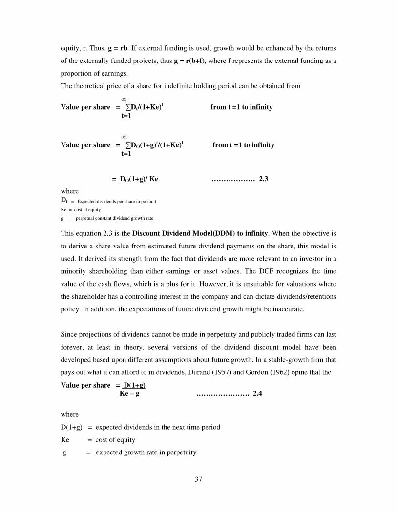
The theoretical price of a share for indefinite holding period can be obtained from
� Value per share = �Dt/(1+Ke)t from t =1 to infinity t=1
� Value per share = �DO(1+g)t/(1+Ke)t from t =1 to infinity t=1
= DO(1+g)/ Ke ……………… 2.3
where Dt = Expected dividends per share in period t
Ke = cost of equity
g = perpetual constant dividend growth rate
This equation 2.3 is the Discount Dividend Model(DDM) to infinity. When the objective is
to derive a share value from estimated future dividend payments on the share, this model is
used. It derived its strength from the fact that dividends are more relevant to an investor in a
minority shareholding than either earnings or asset values. The DCF recognizes the time
value of the cash flows, which is a plus for it. However, it is unsuitable for valuations where
the shareholder has a controlling interest in the company and can dictate dividends/retentions
policy. In addition, the expectations of future dividend growth might be inaccurate.
Since projections of dividends cannot be made in perpetuity and publicly traded firms can last
forever, at least in theory, several versions of the dividend discount model have been
developed based upon different assumptions about future growth. In a stable-growth firm that
pays out what it can afford to in dividends, Durand (1957) and Gordon (1962) opine that the
Value per share = D(1+g) Ke – g …………………. 2.4
where
D(1+g) = expected dividends in the next time period
Ke = cost of equity
g = expected growth rate in perpetuity
38
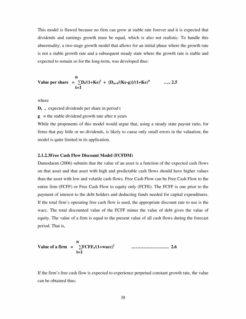
This model is flawed because no firm can grow at stable rate forever and it is expected that
dividends and earnings growth must be equal, which is also not realistic. To handle this
abnormality, a two-stage growth model that allows for an initial phase where the growth rate
is not a stable growth rate and a subsequent steady state where the growth rate is stable and
expected to remain so for the long-term, was developed thus:
n Value per share = �Dt/(1+Ke)t + {Dn+1/(Ke-g)}/(1+Ke)n ….. 2.5 t=1
where
Dt = expected dividends per share in period t
g = the stable dividend growth rate after n years
While the proponents of this model would argue that, using a steady state payout ratio, for
firms that pay little or no dividends, is likely to cause only small errors in the valuation; the
model is quite limited in its application.
2.1.2.3Free Cash Flow Discount Model (FCFDM)
Damodaran (2006) submits that the value of an asset is a function of the expected cash flows
on that asset and that asset with high and predictable cash flows should have higher values
than the asset with low and volatile cash flows. Free Cash Flow can be Free Cash Flow to the
entire firm (FCFF) or Free Cash Flow to equity only (FCFE). The FCFF is one prior to the
payment of interest to the debt holders and deducting funds needed for capital expenditures.
If the total firm’s operating free cash flow is used, the appropriate discount rate to use is the
wacc. The total discounted value of the FCFF minus the value of debt gives the value of
equity. The value of a firm is equal to the present value of all cash flows during the forecast
period. That is,
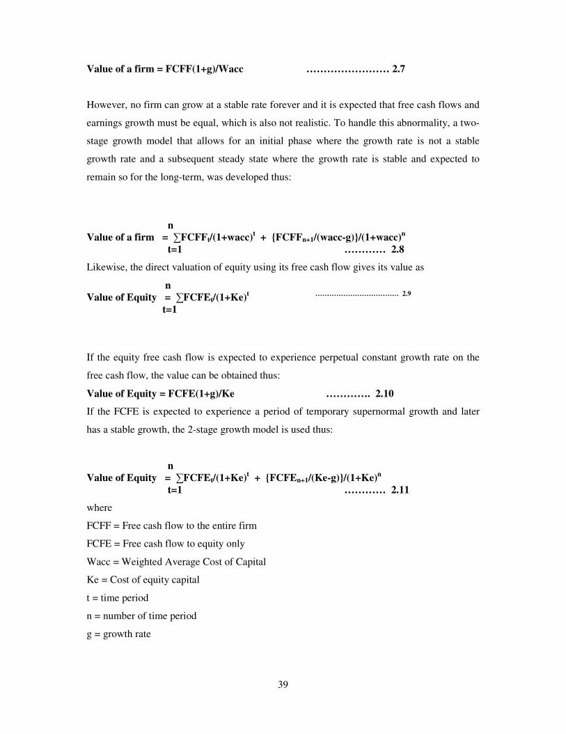
n Value of a firm = �FCFFt/(1+wacc)t ……………………. 2.6 t=1
If the firm’s free cash flow is expected to experience perpetual constant growth rate, the value
can be obtained thus:
39
Value of a firm = FCFF(1+g)/Wacc …………………… 2.7
However, no firm can grow at a stable rate forever and it is expected that free cash flows and
earnings growth must be equal, which is also not realistic. To handle this abnormality, a two-
stage growth model that allows for an initial phase where the growth rate is not a stable
growth rate and a subsequent steady state where the growth rate is stable and expected to
remain so for the long-term, was developed thus:
n Value of a firm = �FCFFt/(1+wacc)t + {FCFFn+1/(wacc-g)}/(1+wacc)n t=1 ………… 2.8
Likewise, the direct valuation of equity using its free cash flow gives its value as
n Value of Equity = �FCFEt/(1+Ke)t ……………………………… 2.9 t=1
If the equity free cash flow is expected to experience perpetual constant growth rate on the
free cash flow, the value can be obtained thus:
Value of Equity = FCFE(1+g)/Ke …………. 2.10
If the FCFE is expected to experience a period of temporary supernormal growth and later
has a stable growth, the 2-stage growth model is used thus:
n Value of Equity = �FCFEt/(1+Ke)t + {FCFEn+1/(Ke-g)}/(1+Ke)n t=1 ………… 2.11
where
FCFF = Free cash flow to the entire firm
FCFE = Free cash flow to equity only
Wacc = Weighted Average Cost of Capital
Ke = Cost of equity capital
t = time period
n = number of time period
g = growth rate
40
The forecast period is the time period for which the individual yearly cash flows are input to
the DCF formula. There are no fixed rules for determining the duration of the forecast period,
and cash flows after the forecast period can be represented by a fixed number such as annual
growth rates. The projected future continuing value is determined using the CFn (1 +
gn)/(wacc – gn). The present value of the continuing value is then obtained by discounting
the projected future continuing value using (1 + waccn)n
2.1.2.4 Relative Valuation Approach
The relative value models determine the value of a firm by observing the prices of similar
companies usually called the guideline companies that sell in the market. That is, the relative
valuation estimates the value of an asset by looking at the pricing of comparable assets
relative to a common variable like earnings, cash flows, book value or sales. The observed
prices serve as valuation benchmarks. From the prices, one calculates price multiples such as
the price-to-earnings or price-to-book value ratios. Next, one or more price multiples are used
to value the firm. For example, the average price-to-earnings multiple of the guideline
companies is applied to the subject firm’s earnings to estimate its value. Many price multiples
can be calculated. Most are based on a financial statement element such as a firm’s earnings
(price-to-earnings) or book value (price-to-book value) but multiples can be based on other
factors such as price-per-subscriber, price-to-cash flow.
An advantage of this approach is that it provides information about how the market is
currently valuing securities at several levels-that is, the aggregate market, alternative
industries, and individual stocks within industries. It generates alternative relative valuation
ratios for the aggregate market, for an industry relative to the market, and for an individual
company relative to the aggregate market, to its industry, and to other stocks in its industry.
Its demerit is that it provides information on current valuation only, and gives no clue on
whether the current valuation is appropriate. However, the relative valuation techniques are
appropriate to consider when there is a good set of comparable entities, and that the aggregate
market and the guideline companies are not either seriously undervalued or overvalued.
2.1.2.5 Earnings Multiplier (P/E Ratio) Model
Based on the reasoning that the value of any investment is the present value of future returns,
and that the returns to common stocks investors are the net earnings of the firm, earnings
multiplier model can be used to determine the value of equity. The earnings multiplier is the

41
absolute number obtained when current price is divided by expected 12-month earnings. That
is, Current Price = Earnings Multiplier (Expected 12-month Earnings). To look at a
company’s earnings relative to its price, most investors employ the P/E ratio. In essence,
earnings multiplier is the number of Naira investors are willing to pay for one Naira of
expected earnings. An analyst can compute the prevailing earnings multipliers and use them
comparatively to determine the value of other comparable stocks based on the earnings, cash
flow, book value, and sales. Trailing P/E ratio, which is Current Price/last 12-month EPS, can
also be used to look for low P/E stocks (ie stocks with very low price relative to their trailing
earnings).
The P/E ratio is an important variable in the valuation of a stock. Its importance is seen in the
earnings capitalization or multiplier approach to stock valuation. The P/E ratio is a common
measure of the esteem in which the company is held by investors. It is the most popular
measure of performance of a stock and the growth prospects of the firm. Stated
mathematically, it is the closing price of the stock divided by the reported earnings of the
most recent twelve months. It is primarily determined by the riskiness of the firm and the rate
of growth in its earnings. Low P/E ratios are associated with low earnings growth and high
P/E ratios are associated with high earnings growth.
2.1.2.6 Price/Earnings to Growth rate ratio (PEG)
PEG is an acronym for Price/Earnings to Growth ratio expressed in percentage, used to see
where a stock traded in the past. It can be computed using forward P/E and annualized
expected earnings growth rate or Historical P/E and annualized historical earnings growth
rate
PEG = Historical P/E Annualized Historical Growth Rate
PEG = Forward P/E Annualized Historical Growth Rate
If the PEG percentage ratio rises above 100% the stock becomes more and more overvalued.
If the PEG falls below 100% the stock becomes more and more undervalue. For instance, a
PEG of 1.0 or 100% suggests that a company is fairly valued. If a stock has a PEG ratio of
0.5 or 50% it implies that it is selling for one-half (50%) of its fair value. If it has a PEG ratio
of 2 or 200% it is selling double its fair value. This theory is based on the belief that P/E
42
ratios approximate the long term growth rate of a company’s earnings. On how to use the peg
ratio, an example suffices.
An investor is thinking about buying stock X or stock Y. Stock X is trading at a forward P/E
of 8 and expected to grow at 10%. Stock Y is trading at a forward P/E of 15 and expected to
grow at 12%. The PEG ratio for stock X is 8/10 = 80% and for Stock Y is 15/12 = 125%.
According to PEG ratio, stock X is a better purchased because it has a lower PEG ratio. In
other words, stock X future earnings growth is purchased for a lower relative price than that
of stock Y, and so it looks cheap.
2.1.2.7 Price/Book value (PBV)
Price / Book value (PBV) = Current price Current Book value The closer the PBV to book value the better it is best suited to takeovers.The ideal ratio is 1.7
to 2.0.
2.1.2.8 Price / Sales ratio (PSR)
This is a revenue based valuation that divides the current market capitalization of a company
by its last 12 months trailing sales revenues. Alternatively it could be current market price per
share divides by the annual sales per share. It is also called multiple of sales. In another form
the long term debt of the company is added to the current market capitalization (to get
enterprise value) before dividing it by the sales revenues. The logic in the later form is that if
one is acquiring the company, he would acquire its debts as well. But in using this valuation
for comparison put away the contribution of debt financing in the sales revenue before
looking for the quotient. The lower the PSR, the better. Ideally a PSR below 1.0 is okay. PSR
shows how much the stock costs per Naira of sales earned. The company with low P/E and
high PSR indicates that some one-time gains are pumping up the EPS. The PSR model is
more appropriate to new companies in hot industries and for acquisition purposes.
Note that Enterprise value = Market Capitalization + Long term and short term debts +
Accounts payable – Accounts Receivable – cash
2.1.2.9 Price/Cash flow Multiple
The ideal range is between 6.0 -7.0, anything above the ideal range is considered expensive in
acquisition assessment. For Leveraged Buyout the ideal is 5.0

43
2.1.2.10Enterprise Value to sales (EVS) ratio
This ratio measures the total company value as compared to its annual net sales. A high ratio
means that the company’s value is much more than its sales. EVS = EV/Sales. EVS is
especially useful when valuing companies that do not have earnings or that are going through
unusually rough times and currently losing money. In this case P/E ratio is irrelevant. EVS
shows what the company could trade for when its rough times are over and its earnings are
back to normal. In this sense an EVS ratio below the normal EVS is ideal.
2.1.2.11EV/ EBITDA (EVE) ratio
The higher the EVE ratio the more expensive the company is. It is one of the best measures
of whether or not a company is cheap or expensive.
2.1.2.12Subscription-member-based valuation
Sometimes a company can be valued based on the number strength of its subscribers. For
example 10million subscribers who averagely spend N1000 per month on services of a
service provider will generate 12 x N1000 x 10m = N12billion per year. So the company is
worth N12billion per year baring entrant of new subscribers and exit of old subscribers. The
method is good for media communication industry, healthcare but their exact mechanics are
unique to each industry. It ignores the past revenues of the company and focus on the
additional revenue to be generated. The analyst will calculate the average revenues per
subscriber over their life time and then figure the value for the entire company.
2.1.2.13Models for setting the offer price
Prior to June 25, 1988, Korean firms were reluctant to go public for two reasons (Jeong-Bon
Kim, 1995). First, the subscription price of an IPO was set using as set of formulae prepared
by the government regulators which did not reflect the true firm value and was in general,
substantially below the value perceived by the market as reported in Kim et al (1993) and
Howe et al (1995). The second reason was that the Korean tax and financial system made
debt financing less costly than equity financing, through ceiling on interest rates and loan
guarantee fees, low interest loans to specific industries, frequent government bailout of large
firms, and favourable tax treatment of debt relative to equity at the corporate and personal
level.

44
Prior to June 25, 1988, the following formulae were used as the basis for setting the
subscription price of an IPO in Korea:
2.1.2.14 Dividends based Value
Price per share (VD) = Average Predicted dividend Interest rate
Where interest rate is the deposit rate for one year.
2.1.2.15 Net Assets based Value
Price per share (VA) = Total net asset + new issue proceeds Total number of shares after IPO
2.1.2.16 Relative Value
VR = Ps x Issuing firm’s per share profit + Issuing firm’s per share net assets 2 Similar firm’s per share profit Similar firm’s per share net assets
Where Ps, is a similar firm’s share price and the price per share is VR. The similar firm must
be in the same industry, have a similar size, etc as the issuing firm. Then the offer price Po,
was set using the following decision criteria.
1. If VR is smaller than or equal to VD (that is VR � VD), then Po = VR
If VR is greater than VD (that is VR > VD), then Po = 0.5 (VR + VD)
2. If VD � VA, then Po = VD
If VD > VA, then Po = 0.75 VD + 0.25 VA
2.1.2.17 Net Book Value of Assets per Share (ie Net Asset Value)
With this method, the value of the assets is adjusted for the value of liabilities due to
outsiders to arrive at the net assets value due to the equity. The net asset value is then divided
by the number of ordinary shares in issue to get the net asset per share. That is, the shares are
valued by taking the net book value of the company’s assets that are financed by equity
capital and dividing this by the number of shares in issue. The net book value of fixed assets
is their value net of depreciation in the books of account and the net book value of current
assets is total current assets minus total current liabilities.
Price per share = Net book value of assets minus External liabilities Number of shares

45
This model is useful when the objective is to relate the value of a share to the company’s
balance sheet. Its strength is in the fact that balance sheet valuations are fairly readily
obtainable. The weaknesses are that balance sheet valuations depend on historical cost
accounting conventions which might be very different from market valuations and the value
of the company and its shares should come mainly from its profits not its asset values.
Balance sheet valuations are unrealistic valuations especially in a period of high inflation.
2.1.2.18 Current Cost of Assets per Share
Shares are valued by taking the current cost value of the company’s assets that are financed
by equity capital and dividing this by the number of shares in issue. The current cost value of
assets is usually their net replacement cost in the case of fixed assets (ie. Replacement cost
minus depreciation) and replacement cost in the case of stocks. However, current cost value
might sometimes be net realizable value.
Price per share = Current cost value of assets minus External liabilities Number of shares
This model is useful when the objective is to relate the value of a share to the current cost
values of the company’s assets. Its strength is that current cost valuation usually gives
realistic figures than balance sheet valuations especially in a period of high inflation. Its
weakness is that current cost valuation of an asset assumes that the business will continue as a
going concern and so a profit based valuation of share must be preferable.
2.1.2.19 Number of Years Purchase of Earnings
This is essentially similar to the price/earnings ratio method and the same objectives,
strengths and weakness apply. It might be used to reach a takeover price where the buyer
agrees to pay the seller a multiple of future earnings. For example, a sale price might be 10
times current year earnings of N1 million with a ‘top up’ in each of the next years of 10 times
the amount by which earnings in those years exceeds N1million
By the method, a share is valued on the basis of a certain number of years of earnings, and so
it is essentially the same as the price/earnings ratio method.
Price per Share = EPS x Agreed number of years earnings
46
Alternatively, it can be used to describe a valuation method whereby shares are valued at say
the total of the last six years earnings or the total of estimated earnings for the next six years.
2.1.2.20 Price/Earnings Multiplier
With this model the share price is regularly measured as a multiple of the company’s earnings
per share (EPS) which is simply the ratio of market price to EPS. A share valuation for any
company can be reached by multiplying a suitable EPS by a suitable P/E ratio. Alternatively,
the P/E ratio of a similar company in terms of risk exposure, size, and class of business is
used to multiply the EPS of the firm that is under valuation. The resulting price is the value of
the ordinary shares of the firm.
Price per share = EPS x P/E ratio
When the objective is to derive a value for a share based on earnings, this is a handy model.
Its strengths are that earnings are more significant than dividend for an investor with a
controlling interest in the company (e.g. A parent company). Again, P/E ratios are widely
used to assess the market prices of companies whose shares are quoted on the stock
exchange. However its weaknesses are that P/E valuation for a share depends on estimates of
suitable values for EPS and market price (P). It is based on forecast earnings.
2.1.2.21 Liquidation Value
Here, the realizable values of the assets are summed together and adjusted for liabilities due
to outsiders. The resultant figure is the value attributable to equity. When the figure is divided
by the number of shares in issue, the quotient is the value per share.
2.1.2.22 Replacement Value
The current costs of replacing the assets are used to value the assets. Adjustment is then made
for liabilities due to outsiders to arrive at the value due to equity. Dividing the net figure by
the number of shares in issue gives the value per share.
2.1.2.23 Stock price relative to treasury bonds
This is the price at which investor can purchase a share at the given EPS to get a return equal
to that of the government bond. The projected stock price relative to treasury bonds is
obtained from the model
Market price per share (MPPS) = Earnings per share (EPS) = EPS Treasury bill rate of return RT

47
Where RT = Treasury bond rate of return
2.1.2.24 Stock price relative to equity value per share
To project stock price relative to equity value per share, let the following be as stated
Equity value per share (EVPS) = Ve
Return on Equity (ROE) = Net Earnings x 100 = Re Shareholders fund 1 Dividend payout rate (DPR) = Dividend per share (DPS) = RP Earnings per share (EPS) Retention Rate (RR) = 1 – DPR = Rr
Equity value per share growth rate = RrRe
EPS at any point in time (t) = EPSt = Et
Equity value per share at any point in time (t) = Vet = Veo (1+RrRe)n
Et = Vet.Re = Veo (1+Rr Re)n Re
Market price per share = MPPS = Et (P/E) = Veo (1+RrRe)n Re(P/E)
2.1.2.25 With constant growth dividend trend to perpetuity
Using securities of comparable risk class the present value of the annual dividend payments
with constant growth to perpetuity is
Po = D(1 + g) r – g where
Po = current price
D = current dividend
D(1+g) = dividend next year
r = capitalization rate or discount rate
g = the constant growth rate
This formula is useable only when r > g. From this model
r = D(1 + g) + g Po That is, the market capitalization rate(r) is equals to the dividend yield D(1+g)/Po plus the
expected rate of growth in dividends (g). The projected growth rate (g) can be estimated from
g = (Latest Dividend/Earliest Dividend)-(n-1) – 1 or from Gordon’s growth model which
states that g = rebe
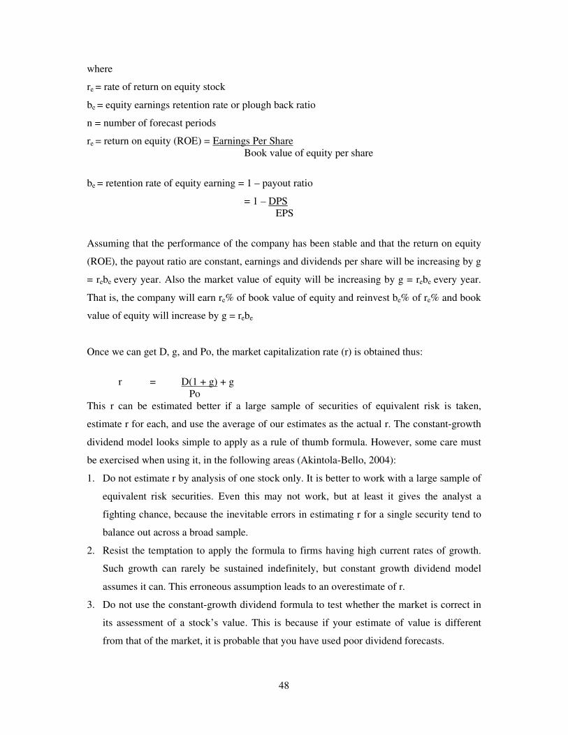
48
where
re = rate of return on equity stock
be = equity earnings retention rate or plough back ratio
n = number of forecast periods
re = return on equity (ROE) = Earnings Per Share Book value of equity per share
be = retention rate of equity earning = 1 – payout ratio
= 1 – DPS EPS
Assuming that the performance of the company has been stable and that the return on equity
(ROE), the payout ratio are constant, earnings and dividends per share will be increasing by g
= rebe every year. Also the market value of equity will be increasing by g = rebe every year.
That is, the company will earn re% of book value of equity and reinvest be% of re% and book
value of equity will increase by g = rebe
Once we can get D, g, and Po, the market capitalization rate (r) is obtained thus:
r = D(1 + g) + g Po This r can be estimated better if a large sample of securities of equivalent risk is taken,
estimate r for each, and use the average of our estimates as the actual r. The constant-growth
dividend model looks simple to apply as a rule of thumb formula. However, some care must
be exercised when using it, in the following areas (Akintola-Bello, 2004):
1. Do not estimate r by analysis of one stock only. It is better to work with a large sample of
equivalent risk securities. Even this may not work, but at least it gives the analyst a
fighting chance, because the inevitable errors in estimating r for a single security tend to
balance out across a broad sample.
2. Resist the temptation to apply the formula to firms having high current rates of growth.
Such growth can rarely be sustained indefinitely, but constant growth dividend model
assumes it can. This erroneous assumption leads to an overestimate of r.
3. Do not use the constant-growth dividend formula to test whether the market is correct in
its assessment of a stock’s value. This is because if your estimate of value is different
from that of the market, it is probable that you have used poor dividend forecasts.

49
The underlying assumptions of the constant-growth dividend model are that
1. The regular future growth rate (g) is at best an approximation
2. Even if the regular future growth rate (g) is an acceptable approximation, errors inevitably
creep into the estimate of g.
3. In well functioning market, investors must capitalize the dividends of all securities in the
same risk class at exactly the same rate (r).
4. Growth has been finance entirely by plough back of certain percentage of earnings.
2.1.2.26 Using Variable Dividend Model (For a definite Period)
In real life, no company can continue to grow at a constant rate per year indefinitely, except
possibly under extreme inflationary condition. Eventually profitability will fall and the
company will respond by investing less. The company can reduce its plough back ratio if the
rate of return declines over time and increase the payout ratio if there are no viable
opportunities. Consequently the value of g will drop. To accommodate this reality, a model
called variable dividend model is churned out. That is,
n Price per share = �Dt/(1+r)t + Pn/(1+r)n t=1
2.1.2.27 Non-Growth, Non-plough back, Constant Dividend stream model
The case of a company that does not grow at all, does not plough back any earnings, but
simply produces a constant stream of dividends is a different ball game. Such a stock is like a
perpetual bond and the return on a perpetual bond is equal to the yearly cash flow divided by
the present value. Therefore, the expected rate of return on a share with no-growth potential,
no-plough back but with constant dividend stream is given as
r = yearly dividend per share = DPS = the dividend yield = D Share price Po Po Since all earnings are paid out as dividends, the expected return is also equal to
r = yearly earnings per share = Earnings yield = EPS Share price Po
The discount rate used is generally the appropriate cost of capital. If the free cash flows to a
firm are the cash flows from the total assets before any debt payments (EBIT) minus
reinvestment in assets to create future growth, then the discount rate that is appropriate is that
which reflects the composite cost of financing from all sources of capital, and this is the
weighted average cost of capital (wacc). This discount rate reflects the cost of raising both

50
debt and equity financing, in proportion to their use. The present value obtained using these
free-cash-flows and the discount rate is the value of the firm which reflects the value of all
claims on the firm. This approach is called the Entity or Firm Valuation approach. If the Free
Cash Flows are the cash flows after debt payments (EAIT) minus needed reinvestment in
assets to create future growth, they are called Free-Cash-Flows-to-Equity, and then the
discount rate that is appropriate is the one that reflects only the cost of equity financing which
is the cost of equity capital. The present value obtained with this approach is called the value
of equity claims on the firm. This approach is called the equity valuation approach.
We can always get the firm value to the equity value by netting out the value of all non-
equity claims from firm value. If done right, the value of equity should be the same whether it
is valued directly (by discounting cash flows to equity at cost of equity) or indirectly (by
valuing the firm and subtracting out the value of all non-equity claims).
2.1.3 Sentiments that Affect Stock Value
2.1.3.1 Investors Preferences
Investors differ in their needs and goals. Each investor chooses the form of investment that
meets his specific objective which could be income, capital appreciation, and preservation of
capital or a combination of all. An investor whose objective is income should go to income
stocks that pay relatively large proportion of its earnings in dividends. Investors pursuing
capital appreciation objective invest in stocks of firms that are growing very rapidly and
consequently retaining a large percent of their earnings for expansion purposes. The investor
receives little or no dividend in any operating year but the growth potential provides him with
a substantial return in later periods. An investor with both income and capital appreciation
objectives who places more emphasis on income and less on appreciation goes for stocks that
provide a fairly high dividend yield with a moderate appreciation potential. The investor with
both income and capital appreciation who places more emphasis on capital appreciation than
income goes for stocks with relatively good appreciation potential but with only a moderate
dividend yield.
Investors in shares can be classified into passive and active investors. The passive investors
are those who buy shares for keeps, never care to find out what is happening in the shares
business but content with the dividend and bonuses they receive. The active investors are

51
those who buy shares for speculative purposes. That is, they buy when it is cheap and sell
when the price rises, and care for what is happening in the shares market. The selection of
securities to make up an investment portfolio that suits the investor’s need of achieving a
higher return subject to a given risk level or a lower risk subject to a given level of return also
affect investor’s preference for any share.
Stock market behaviour has featured prominently in the development of modern theories of
what determines the market price and value of securities. The most popular of the modern
theories underlying share pricing are discussed below.
2.1.3.2 Fundamental Analysis
Fundamental analysis is a method of evaluating securities by measuring the intrinsic value
using real data such as revenue, earning, future growth, return on equity, profit margins, and
others obtained from the company’s financial statements. It studies everything from the
overall economy and industry conditions to the financial conditions and management of the
companies (Olukoya 2004:11). It relies on historical information on earnings, dividends,
capital appreciation, etc. With the trend made from this past information, attempt is made to
predict the future performance of the entity from which the price per share is determined.
2.1.3.3 Technical Analysis
This is a technique used to predict the future movements of share price based on past trends
without taking cognizance of the factors that have led to the movements. It uses the stock
market statistics such as prices and volumes, supply and demand to predict changes in the
market prices of shares. The concept makes use of relative strength, filter rules and charts to
buttress its argument. That is, Technical analysts assume that the past behaviour of a
security’s price tends to reoccur in the future and that careful analysis of stock price averages
and the price of individual shares reveal important data concerning future price movements.
Filter rules usually require the investor to buy if a security’s price goes up at least Y percent
and sell when it declines by X percent or more.
2.1.3.4 Random Walk Hypothesis
This is a term used in mathematics and statistics to describe a process in which successive
elements in a data series are independent of each other and therefore is essentially random
and unpredictable. The RWH applied to the valuation of stocks says that future path of

52
individual stock prices is no more predictable than the path of a series of random numbers. It
assumes that each stock has an intrinsic value based on investors’ expectations of the
discounted value of future cash flows generated by that stock. It believes that the market price
per share is an unbiased estimator of a stock’s intrinsic value and reflects the latest
information available concerning the issuing company’s condition and future prospects.
Hence the successive changes in the price of a stock are random fluctuations around that
stock’s intrinsic and these changes are independent of the sequence of price changes that
occurred in the past. In effect, stock price changes act as though they were independent
random drawings from an infinite pool of possible prices. This school of thought disagrees
with the technical analysts belief of using past share price movement to predict the future
prices. It conceives the notion that changes in the share price occurs at random, so there is no
relationship between prices of share in the past and in the future. Knowledge of the sequence
of Past share price prior to the current time period contains little or no information about the
direction of future share price and the information on new share price appears in random
fashion. It adopts the saying that “price has no memory, yesterday has nothing to do with
tomorrow, every day starts out fifty-fifty, and yesterday price discounted everything
yesterday. Empirical evidence from research studies by Fisher and Lorie (1964), Madelbrot
(1963), Fama (1965), Granger and Morgensten (1970) do not indicate any meaningful degree
of dependence of future stock price movements on those occurring in the past.
2.1.3.5 Noise Trading
This is a term used to explain the situation where stock prices deviate from their fundamental
values as a result of the buy and sell positions of uninformed investors. And the situation may
not be corrected if the informed investors are willing to capitalize on the discrepancy.
2.1.3.6 The Efficient Market
A market is efficient if scarce resources are allocated to their most productive uses. Prices of
scarce resources fluctuate randomly around their intrinsic values and are always in
equilibrium and any temporary deviations from equilibrium prices are quickly corrected. As
prices adjust instantaneously to new information, a new set of intrinsic values result, leading
some investors to adjust their portfolios. Therefore, as latest information is reflected in
resources prices, market price always equals intrinsic value in a state of continuous
equilibrium, which strongly supports the view of RWH. Applied to securities market, the
efficient market is one where security prices quickly and fully reflect all available

53
information. In this market the same return is available for the same level of risk. In an
efficient capital market at each point in time, all securities in an equivalent risk class are
priced to offer the same expected return. This is a condition for equilibrium in well-
functioning capital market. Any stock that offers above the normal price should offer above
the normal income to generate a higher rate in return. If not, at that above-the-normal price
the stock will offer a rate of return that is lower than those other securities of equivalent risk.
With this lower rate of return, investors would shift their capital to other securities and in the
process force down the price of the overpriced stock.
Any stock that offers less than normal price should offer less than normal income to generate
a lower rate of return. If the stock offers a higher rate of return than comparable securities,
investors would rush to buy it forcing the price up.
2.2 Survey of Related Studies
Valuation can be considered the heart of finance as it lies at the heart of much of what we do
in finance (Damodaran (2006). Understanding what determines the value of a firm and how
to estimate that value seems to be a prerequisite for making sensible investment decisions.
Analysts use a wide spectrum of models, with different assumptions about the determinants
of true values. In general term, the three approaches to valuation are the (1) Discounted cash
flow valuation, which relates the value of an asset to the present value of expected future cash
flows on that asset; (2) relative valuation, which is the pricing of comparable assets relative to
a common variable like earnings cash flows, book value or sales; (3) accounting and
liquidation valuation, which relates the value to the accounting estimates of the value of the
existing assets of a firm. Among the three, DCF approach gets the most play in academic and
comes with the best theoretical credentials.
The earliest interest rate tables were prepared by Francesco Balducci Pegolotti, a Florentine
merchant and politician in 1340 as part of his manuscript titled ‘Practica della mercatura’ but
officially published in 1776 (Parker 1968). The application of present value to valuation can
be traced to both commercial and intellectual impulses. On the commercial side, when there
was a demand for new tools to analyze long-term investments in the United States railroads,
with significant cash outflows in the early years and positive cash flows in later years of

54
second half of the nineteenth century, a civil engineer, Wellington (1887) suggested that the
present value of the future cash flows should be compared to the cost of up-front investment.
Bohm-Bawerk (1903) provided an explicit example of present value calculations using the
example of a house purchase with twenty annual installment payments. To examine whether
to install new machinery or retain the old equipment, Pernnel (1914), an engineer of
Southwestern Bell, developed the present value equations for annuities.
On the intellectual side, the principles of modern valuation were developed by Irving Fisher
in his two books- “The Rate of interest” (1907) and ‘The Theory of Interest’ (1930). In these
books, he suggested four alternative approaches for analyzing investment that he claimed
would yield the same results. He argued that when confronted with multiple investments, one
should pick the investment that (1) has the highest present value at the market interest rate;
(2) has the highest net present value of the benefits over the present value of the costs; (3) has
the highest internal rate of return (IRR) that exceeds the market interest rate (MIR), (4) when
compared to the next most costly investment, yield a rate of return over cost that exceeds the
market interest rate.
The DCF later extends its reach into security and business valuation. The first set of models
under the DCF consider only dividends to be the cash flows to equity, thus discounted only
dividends stream to generate the intrinsic value, hence the name “Dividend Discount Model
(DDM)”. Under the DDM we have constant dividend Discount Model (CDDM) and constant
Growth Dividend Discounted Model (CGDDM).
The DDM is premise on the fact that when investors buy stock in publicly trade firms, they
generally expect to get two types of cash flows namely, the dividends during the holding
period and an expected price gain at the end of the holding period. Since this expected price
gain is itself determined by future dividends, the value of a stock is the present value (PV) of
dividends through infinity, hence the model
� Price per share = �Dt/(1+Ke)t t=1 where
Dt = Expected Dividend per share in period t
Ke = Cost of Equity

55
The basic inputs to the model are the expected dividends and the cost of equity. To obtain the
expected dividends, we make assumptions about future growth rates in earnings and payout
ratios. However the projections of dividend amounts cannot be made in perpetuity but at
least, in theory, publicly traded firms are assumed to last forever. Based on these facts several
versions of DDM have been developed with their respective assumptions about future
growth. For example Durand (1957) and Gordon (1962) opine that in a stable – Dividend
growth firm the
Value of the stock = Dn+1/(Ke – g)
Where
Dn+1 = Expected Dividends next period
Ke = cost of equity
g = Expected growth rate in perpetuity
The Gordon Growth model submits that g = rb
r = rate of return
b = retention ratio
The model is meant to be used on the firms growing at stable rates that can be sustained
forever, and which cannot exceed the growth rate of the economy in which the firm operates.
Again the earnings growth rates and the dividend growth rates are expected to be the same, so
that dividends will not exceed earnings over time. Another reason for the need of the growth
rate equality is that if earnings grow at a faster rate than dividends in the long run, the payout
ratio will converge to zero hence not being stable.
In response to the desire to accommodate situations where there are stable and unstable
growth phases, a two – stage growth model was developed. In the model, the value of a stock
during the non-stable growth phase is given as
n Price per share = �Dt/(1+Ke)t t=1
While the value of the stock at the end of the unstable growth phase is given as
Dn+1/(Ke – g)
Where g = the stable growth rate after n years of unstable growth phase. Therefore the value
of a stock over the two stages is

56
n Price per share = �Dt/(1+Ke)t + Dn+1/(Ke – g) t=1
Though DDM does have its proponents but many analysts argue that its focus is too narrow
and that it yields estimates of value that are far too conservative. It is commended for its
simplicity and intuitive logic. After all, dividends remain the only cash flow from the firm
that is tangible to investors. The estimates for free cash flows to equity and the firm remain
estimates and conservative investors can reasonably argue that they cannot lay claim on these
cash flows. Again we need to make fewer assumptions to get to forecasted dividends than to
get forecasted free cash flows. Fama and French (2001) conclude that firms became less
likely to pay dividends over the period of 1978 to 1999 because of the emergence of many
small cap, high growth firms in 1999 than 1978. DeAngelo, DeAngelo and Skinner (2004)
argue that aggregate dividends paid by companies has not decreased and that the decreasing
dividend can be traced to smaller firms that are uninterested in paying dividends. Baker and
Wurgler (2004) provide a behavioral rationale by pointing out that the decrease in dividends
over time can be attributed to an increasing segment of investors who do not want dividends.
Hoberg and Prabhala (2005) posit that the decrease in dividends is because of increases in
idiosyncratic risk (rather than dividend clientele). From these comments it is obvious that
firms often choose not to pay commensurate dividend relative to the cash available for such
purpose, and this creates a challenge to those who use DDM.
Notwithstanding its limitations, the DDM can be useful in three Scenarios.
1. It establishes a baseline or floor value for firms that have cash flows to equity that
exceeds dividends. For these firms, the DDM will yield a conservative estimate of
value, on the assumption that the cash not paid out by managers will be wasted on poor
investments or acquisitions.
2. It yields realistic estimates of value per share for firms that do pay out their free cash
flow to equity as dividends, at least on average, over time.
3. It is appropriate to use in sectors where cash flow estimation is difficult or impossible.
The true measure of a valuation model is how well it works in explaining differences in the
pricing of assets at any point in time and across time and how quickly difference between
57
model and market prices get resolved. Researchers have come to mixed conclusions on the
first question. Shiller (1981) presents evidence that the volatility in stock prices is far too high
to be explained by variance in dividends over time. In other words, market prices vary far
more than the present value of dividends. In an attempt to explain the excess market
volatility, Poterba and Summers (1988) argue that risk premiums can change over time; Fama
and French (1988) note that dividends yields are much more variable than dividends. Looking
at a much longer time period (1871 – 2003), Forester and Sapp (2005) find that the DDM
does a reasonably good job of explaining variations in the S & P 500 index, though there are
systematic differences over time in how investors value future dividends.
To answer the second question Sorensen and Williamson (1985) valued 150 stocks from the
S & P 500 in December 1980, using the DDM. They used the difference between the market
price at the time and the model value to form five portfolios based upon the degree of under
or over valuation. They made the following assumptions in using the DDM.
1. The average of the earnings per share between 1976 and 1980 was used as the current
earnings per share.
2. The cost of equity was estimated using the CAPM
3. The extraordinary growth period was assumed to be 5 years for all stocks and the 1/B/E/S
consensus analyst forecast of earnings growth was used as the growth rate for this period.
4. The stable growth rate, after the extraordinary growth period, was assumed to be 8% for
all stocks.
5. The payout ratio was assumed to be 45% for all stocks.
The returns on these five portfolios were estimated for the following two years (January 1981
– January 1983) and excess returns were estimated relative to the S & P 500 index using the
betas estimated at that first stage. The undervalued portfolio had a positive excess return of
16% per annum between 1981 and 1983, while the overvalued portfolio had negative excess
return of almost 20% per annum during the same period. In the long run, undervalued
(overvalued) stock from the DDM outperform (underperforms) the market index on a risk-
adjusted basis.
To fix this problem of DDM, free cash flow to equity is used to replacing the dividends in the
DDM as a proxy for potential dividends. The free cash flow represent a smoothed out
58
measure of what firms can return to their stockholders over time in the form of dividends and
other forms. With this the value of equity, under the constant growth model is
Ve = FCFEn+1/(Ke – g)
This gives more realistic estimates of value for equity for firms whose dividends are
significantly higher or lower than the Free Cash flow to equity.
Earnings Models
The failure of companies to pay out what they can afford to in dividends and the difficulties
associated with estimating cash flows has led some to argue that firms are best valued by
discounting earnings or variants of earnings. Ohlson (1995) starts with the DDM but adds on
overlay of what he terms a “clean surplus” relation, where the goodwill on the balance sheet
represents the present value of future abnormal earnings. He goes on to show that the value of
a stock can be written in terms of its book value and capitalized current earnings, adjusted for
dividends. Feltham and Ohlson (1995) build on the same argument to establish a relationship
between value and earnings. Penman and Sougiannis (1997) also argue that Generally Agreed
Accounting Practice earning can be substituted for dividends in equity valuation, as long as
analysts reduce future earnings and book value to reflect dividend payments. But discounting
earnings as if they were cash flows paid out to stockholders and at the same time counting the
growth that is created by reinvesting those earnings amount to double counting and will lead
to overvaluation of stocks.
Another dimension to equity valuation is to value the entire business by discounting the free
cash flow to the firm at before-tax WACC and then remove the debt value. The origin of the
firm valuation model lie in one of corporate finance’s most cited papers by Miller and
Modighani (1958) where they note that the value of a firm can be written as the present value
of its after-tax operating cash flows. A firm with a stable growth rate that can be sustained in
perpetuity can be valued using
Ve = FCFFn+1/(wacc – gn)
Where
EFCFn+1 = Expected free cash flow to the firm next year
Wacc = Weighted Average cost of Capital
gn = Growth rate in the free cash flow to the firm (Forever)

59
The general version of the model can be written as the present value of expected free cash
flows to the firm that is,
� Ve = � FCFFt/(1+wacc)t t=1 If the firm reaches a steady state after n years and starts growing at a stable growth rate gn
after that, the value of the firm can be written as
Value of Operating Assets of the Firm =
� � FCFFt/(1+wacc)t + [FCFFn+1/(wacc-gn)t]/(1+wacc)t t=1
To get to the value of equity from the value of operating assets we have to first incorporate
the value of non-operating assets that are owned by the firm and then subtract all non-equity
claims that may be outstanding against the firm. Non-operating assets include all assets
whose earnings are not counted as part of the operating income. The most common of the
non-operating assets is cash and marketable securities.
2.2.1Certainty Equivalent Models
Some analysts prefer to adjust the expected cash flows for risk with the certainty equivalent
cash flows instead of adjusting the discount rate for risk. Gregory (1978) derives certainty
equivalent function and examines the behaviour. A more practical approach to converting
uncertain cash flows into certainty equivalents is offered by risk and return models. Here
Certainty Equivalent cash flow = Expected cash flow/(1 + Risk premium)
The Risk Premium = (1 + Risk Adjusted Discount Rate)/(1 + Risk free Rate) – 1
In general form, if r = risk adjusted return, rf = risk-free rate, and the certainty equivalent cash
flow = �CF, the expected cash flow = ECFt
�CF = ECFt/(1+{(1+r)/(1+ rf)}-1) = ECFt/((1+r)/(1+ rf))
= ECFt(1+ rf)/(1+r)
For year one, �CF1 = ECF1(1+ rf)/(1+r)
60
For year two, �CF2 = ECF2(1+ rf)2/(1+r)2
For year three, �CF3 = ECF3(1+ rf)3/(1+r) and so on
This process is repeated for all of the expected cash flows, hence the general formula
�CFt = ECFt (1 + rf)t/(1+r)t
However, a more common approximation used by many analysts is the difference between
the risk-adjusted discount rate and the risk-free rate, that is r – rf. But if we use the risk
premium from risk and return model to compute certainty equivalents, the NPV obtained will
be the same as that obtained by adjusting the discount rate for risk (Stapleton 1971).
2.2.2Excess Return Models
Excess return is the difference between the required or actual return cash flows and the
normal return cash flows. The normal return cash flow is equal to earning the risk adjusted
required return. With the excess return valuation framework, the value of business can be
written as the sum of two components:
Value of business = Capital invested in firm today plus present value of excess return
cash flows from both existing and future projects.
The excess return models believe that an investment adds value to a business if it has positive
NPV which had been the target of capital budgeting. And the positive NPV would come if
the investment generates excess return (that is, return on equity capital that exceed the cost of
equity capital). A widely used variant of excess return model is the Economic Value Added
(EVA). This is a measure of the surplus value created by an investment or a portfolio of
investments over the capital invested in that investment or portfolio of investments.
EVA = (Return on capital invested-cost capital)(capital invested) which is equivalent to EVA
= After-tax operating income – (cost capital)(capital invested). According Damodaran
(1999), the
n NPV of EVA = � EVAt/(1+Ke)t t=1 According to Brealey and Myers (2003)
Firm value = Value of Assets in place + value of expected future growth
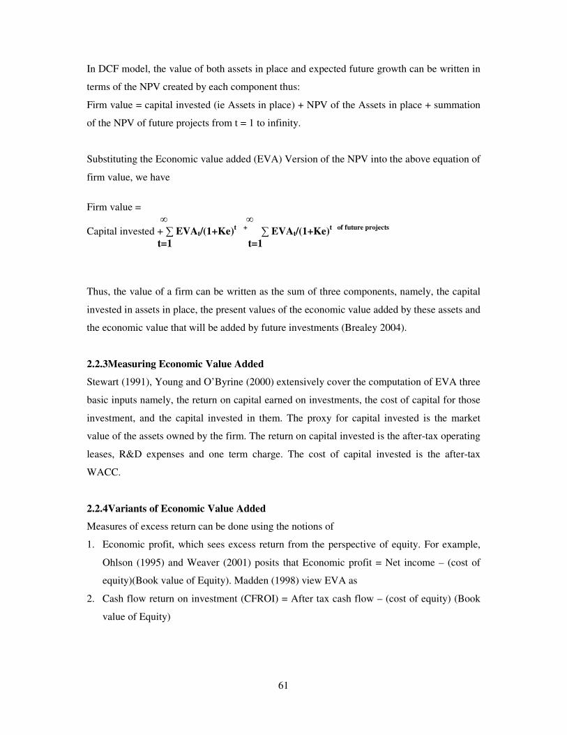
61
In DCF model, the value of both assets in place and expected future growth can be written in
terms of the NPV created by each component thus:
Firm value = capital invested (ie Assets in place) + NPV of the Assets in place + summation
of the NPV of future projects from t = 1 to infinity.
Substituting the Economic value added (EVA) Version of the NPV into the above equation of
firm value, we have
Firm value = � � Capital invested + � EVAt/(1+Ke)t +
� EVAt/(1+Ke)t of future projects t=1 t=1
Thus, the value of a firm can be written as the sum of three components, namely, the capital
invested in assets in place, the present values of the economic value added by these assets and
the economic value that will be added by future investments (Brealey 2004).
2.2.3Measuring Economic Value Added
Stewart (1991), Young and O’Byrine (2000) extensively cover the computation of EVA three
basic inputs namely, the return on capital earned on investments, the cost of capital for those
investment, and the capital invested in them. The proxy for capital invested is the market
value of the assets owned by the firm. The return on capital invested is the after-tax operating
leases, R&D expenses and one term charge. The cost of capital invested is the after-tax
WACC.
2.2.4Variants of Economic Value Added
Measures of excess return can be done using the notions of
1. Economic profit, which sees excess return from the perspective of equity. For example,
Ohlson (1995) and Weaver (2001) posits that Economic profit = Net income – (cost of
equity)(Book value of Equity). Madden (1998) view EVA as
2. Cash flow return on investment (CFROI) = After tax cash flow – (cost of equity) (Book
value of Equity)
62
While proponents of each measure claim its superiority, they agree on far more than they
disagree on. The works of Fernandez (2002), Hartman (2000), Shrives and Wachowicz
(2000), Feltham and Ohlson (1995), Penman (1998), Lundholm and O’keefe (2001) provide
proof that equity excess return models converge on equity discounted cash flow model.
The model values can diverge because of difference in assumptions and ease of estimation.
Penman and Sourgiannis (1998) compared the DDM to excess return models and concluded
that the valuation errors in a DCF model, with a ten-year horizon, significantly exceeded the
errors in an excess return model. They attributed the difference to GAAP accrual earnings
being more informative than either cash flow or dividend. Francis, Olsson and Oswald (2001)
concurred with Penman and also found that excess return models outperform DDMs.
Courteau, Kao and Richardson (2001) argue that the superiority of excess return models in
these studies can be attributed entirely to differences in the terminal value calculation and that
using a terminal price estimated by value line (instead of estimating one) results in DDMs
outperforming excess return models.
2.2.5Adjusted Present Value (APV) Models
The adjusted present value (APV) approach was first presented in Myers (1974) in the
context of examining the interrelationship between investments and financing decisions. It is
built on the presumption that it is easier and more precise to compute the valuation impact of
debt in absolute terms rather than in proportional terms. In APV model the value of the firm
is estimated in three steps: (1) Estimate the firm value with no leverage (2) find the present
value of the interest tax savings generated by borrowing a given amount of money, (3)
compute the effect of borrowing the amount on the probability that the firm will go bankrupt,
and the expected cost of bankruptcy. After these, the value of a firm can be written as
follows.
Value of firm = value of firm with 100% equity financing + present value of expected tax
benefits of debt – expected bankruptcy costs.
Valuing the firm as if it had not debt, we discount the expected free cash flow to the firm at
the unlevered cost of equity. In the special case where cash flows grow at a constant rate in
perpetuity, the value of the firm is easily computed thus:
Value of unlevered firm = EFCFFo (1 + g)/(Keu – g)
63
Where
EFCFFo = current after-tax operating cash flow to the firm
Keu = unlevered cost of equity
g = the expected growth rate
In the more general case, Damodaran (2006:44) states that we can value the firm using any
set of growth assumptions we believe are reasonable for the firm.
The first attempt to isolate the effect of tax benefits from borrowing was in Miller and
Modigliani (1963), where they valued the present value of the tax savings in debt as a
perpetuity using the cost of debt as the discount rate thus:
� Value of tax benefits = � {Tax rate(Interest rate)(Debt)}/(1+Kd)t t=1
� Value of tax benefits = � {T(Kd)(D)}/(1+Kd)t t=1
Where
D = Amount of debt (constant)
Kd = rate of interest on debt (constant)
t = Time period
T = tax rate (company tax rate in Nigeria is 30% constant)
Fernandez (2004) argued that the value of tax benefits should be computed as the difference
between the value of the levered firm, with the interest tax savings, and the value of the same
firm without leverage. Consequently, he arrives at a much higher value for the tax savings
than the conventional approach, by a multiple of the unlevered firm’s cost of equity to the
cost debt. Cooper and Nyborg (2006) argue that Fernandez is wrong and that the value of the
tax shield is the present value of the interest tax savings, discounted back at the cost of debt.
The present value of expected bankruptcy cost is
= (Probability of Bankruptcy) (Present value of Bankruptcy cost)
= P (PBC)

64
The step of the adjusted present value approach poses the most significant estimation
problem, since neither the probability of bankruptcy nor the bankruptcy cost can be estimated
directly. There are direct and indirect costs of bankruptcy. In his study of railroad
bankruptcies, Warner (1977) looked at the direct cost of bankruptcy and concludes that they
are small (about 5%) relative to firm value. Indirect cost of bankruptcy consists of loss of
goodwill on perception of distress, as employees, customers, suppliers and lenders react
leading to loss of customers with loss of sales, higher employee turnover, and tighter
restriction from suppliers etc. Opler and Titman (1994), Andreode and Kaplan (1998)
examine the theory behind indirect bankruptcy costs and estimate using highly levered
transactions that subsequently became distressed and conclude that the magnitude of these
cost ranges from 10 – 25% of firm value.
The probability of bankruptcy can be estimated indirectly into two basic ways. One is to
estimate a bond rating at each level of debt and use the empirical estimates of default
probabilities for each rating. The other one is to use a statistical approach to estimate the
probability of default, based upon the firm’s observable characteristics, at each level of debt.
Value of levered firm = FCFFo (1+g)/(Keu – g) + TD – P(PBC)
In practice, bankruptcy cost is often ignored (Damodaran 2006: 48).
2.2.6Variants of APV
Luehrman (1997), Kaplan and Ruback (1995) suggest use of debt amount changing over time
as a fraction of book value and capital cash flows to both debt and equity, respectively.
2.2.7Asset-based valuations
In asset based valuation, we estimate the value of each asset separately and add them to
obtain value of the business. Valuing a business on a going concern basis we recognize the
existing assets generating cash flows today and expected value from future investment. For
growth prone companies, asset – based valuations yields lower values than going concern
valuations.
2.2.8Accounting Valuations
2.2.8.1Book value Based Valuation

65
Ben Graham (1949) in his “The intelligent investor” states that a stock is under valued if its
market price falls below its book value. Similarly funds that invest in low price to book value
stocks are categorized as value funds. Fama and French (1992) fed into this belief by
presenting evidence that low price to book value stock do earn higher returns than the rest of
the market.
The question therefore is, does book value less the accumulation deprecation the reasonable
proxy for the true value of a business? For mature, non-growth prone firms, yes but for firm
with significant growth opportunities which can generate excess returns, book values will be
very different from true value.
2.2.8.2 Book Value plus Earnings valuation model
Ohlson (1995) basic model states the true value of equity as a function of its book value of
equity and the excess returns on equity that the firm can generate in the future. As a
consequence, it is termed a residual income model and can be derived from a simple DDM.
� Value of equity = �Do(1+g)t/(1+Ke)t t=1 Feltham and Ohlson (1995) suggest that the
Value of equity = Equity Book value t-1 + Net Incomet – Dividendst
Substituting back into the DDM we have Value of equity =
� Equity Book value t-1 +�Net Income - Equity Book value t-1 (Ke) t=1 (1+Ke)t
Thus, the value of equity in a firm is the sum of the current book value of equity and the
present value of the expected excess returns to equity investors in perpetuity.
Walter (1966) followed Ohlson (1995)’s residual income model and modified the DDM to
incorporate excess returns earned on future investment opportunities as follows: Value of
Equity = {D + ROE/Ke(E – D)}/Ke
Where
E = Expected Earnings in the next period
D = Dividends in the next period
ROE = Expected return on equity in perpetuity on retained earnings
Ke = Cost of equity
66
ROE/Ke(E – D) = Excess return generated on an annual basic divided by the cost of equity to
yield its present value in perpetuity.
Mao (1974) capitalized current earnings (as perpetuity) and called the value the book value of
equity, and then added the present value of future excess returns to this value. That is, Value
of Equity = E/Ke + ROE/Ke (E – D)
Lundholm and O’keefe (2001) show that DCF models and Ohlson’s residual income models
yield identical valuations of companies if we make consistent assumptions. Ohlson’s model
has followers because it allowed accountant to argue that accounting numbers are still
relevant to value. After all, Lev (1989) had presented evidence on the declining significance
of accounting earnings numbers by noting a drop in the correlation between market value and
earnings. The works of Frankel and Lee (1996), Hand and Landsman (1998), Dechow,
Hutton and Sloan (1999) find that the residual income model explains 70 – 80% of variation
in prices across stocks.
2.2.8.3 Fair Value Accounting
The question here is do fair value judgments made by accountants provide information to
financial market or do they just muddy up waters? Barth (1994) concludes that fair value
accounting provided useful information to markets in a variety of contexts. In contrast Nelson
(1996) examines fair value accounting in banking where marking to market has been
convention for a much longer period, and finds the reported fair values of investment
securities have little incremental explanatory power when it come to market values. Chen
Kohlbeck and Warfield (2004) find that stock prices react negatively to goodwill
impairments, may be along with other interpretations, but are a weak evidence to show that
fair value accounting assessments conveys information to markets.
2.2.8.4 Liquidation Valuation
This is an asset based valuation where we value assets based upon the presumption that they
have to be urgently sold now. It is common to see analysts assume that liquidation value will
be a specified percentage of book value. Berger, Ofek, and Swary (1996) argue and provide
evidence that book value operates as a proxy for abandonment value in many firms. Lang,
stulz and Walkling (1989) use book value as a proxy for the replacement cost of assets when
computing Tobin’s Q. Tobin’s Q is the ratio of the value of the firm to replacement cost.

67
The liquidation value should be significantly lower than the DCF value, partly because the
latter reflects the value of expected growth potential and the former usually do not. In
addition, the urgency associated with the liquidation can have an impact on the proceeds,
since the discount on value can be considerable for those sellers who are eager to divest their
assets. Kaplan (1989) cited a Merrill Iynch estimate that the speedy sales of the Compeau
stake in Federated would bring about 32% less than an orderly sale of the same assets.
Holland (1990) estimates the discount to be greater than 50% in the liquidation of the assets
of machine tool manufacture. Willianson (1988), makes the very legitimate point that the
extent of the discount is likely to be smaller for assets that are not specialized and can be
redeployed elsewhere. Shleifer and Vishny (1992) argue that assets with few potential buyers
or buyers who are financially constrained are likely to sell at significant discounts on market
value.
In summary, liquidation valuation is likely to yield more realistic estimated of value for firms
that are distressed, where the going concern assumption underlying conventional DCF
valuation is clearly violated for healthy firms with significant growth opportunities, it will
provide estimates of values that are far too conservative.
2.2.9 Relative Valuation
In relative valuation, we value an asset based upon how similar assets are priced in the
market. A prospective automobile buyer decides how much to pay for a car by looking at the
prices paid for similar cars in the neighbourhood. A land buyer makes a judgment on how
much to pay for a parcel of land by checking land transaction prices on similar lands in
comparable vicinity. In the same vein, a potential investor in a stock tries to estimate its value
by looking at the market pricing of similar stocks. The essential steps in relative valuation are
as follows:
1. Finding comparable assets that are priced by the market. Some analysts use sector or
industry.
2. Sealing the market price to a common variable to generate standardized price that are
comparable. This is necessary when comparing assets that vary in size or units. Other
things being equal, a smaller house or apartment should trade at a lower price than a
larger residence. In the context of stocks, this equalization usually requires converting the
market value of equity or the firm into multiples of earnings, book value or revenues.
68
3. Adjusting for difference across assets when comparing their standardized valued. For
instance, a newer house with more updated amenities should be priced higher than a
similar sized older house that needs renovation. With stocks, differences in pricing across
stocks can be attributed to the entire fundamental like growth opportunities, book value.
Hhigher growth companies should trade at higher multiples than lower growth companies
in the same sector.
In standardizing values, one of the more intuitive ways to think of the value of any asset is as
a multiple of the earnings that asset generates. When buying a stock, it is common to look at
the price paid as a multiple of the EPS generated by the company. This price/earnings ratio
can be estimated using current earnings per share, EPS to yield a current P/E, or using
earnings over the last 4 quarter to yield a trailing P/E, or an expected EPS in the next year to
provide a forward P/E. When buying a business as opposed to just the equity in the business,
it is common to examine the value of the firm as a multiple of the operating income or the
earnings before interest, taxes, depreciation and amortization (EBITDA). As a buyer of the
equity or the firm, a lower multiple is better than a higher one.
Price/book value of equity (or net worth) ratio is also a measure of how over or undervalued a
stock is but this varies widely across industries. Because of the wide gyration, Tobin’s Q is
preferred. Tobin’s Q is the ratio of the value of the firm to Replacement cost.
The PE and PBV ratio are affected by choice of accounting rules and principles. To get off
the hook of such accounting choice, the use of the ratio of the value of a business to the
revenues it generates is preferred. In this sense for equity investors, this ratio is the price /
sales ratio (PS), where the market value of equity is divided by the revenues generated by the
firm. For firm value, this ratio is modified as the enterprise value / sales ratio (VS), where the
numerator becomes the market value of the operating assets of the firm. This ratio again
varies widely across sectors, largely as a function of the profit margins in each.
The advantage of using revenue multiples, however, is that it becomes far easier to compare
firms in different markets, with different accounting systems at work, than it is to compare
earnings or book value multiples.
Multiples that are specific to a sector include market value / customer ratio, market value /
subscriber ratio. These sector-specific multiples lack general applicability because they
cannot be computed for other sectors or for the entire market. Secondly it is far more difficult
69
to relate sector-specific multiples to fundamentals, which is an essential ingredient to using
multiples well.
There have been relatively few studies that document the usage statistic on these multiples
and compare their relative efficiency. Damodaran (2002) notes that the usage of multiples
varies widely across sectors, with Enterprise value / EBITDA multiples dominating
valuations of heavy infrastructure businesses (like cable, telecomm) and price to book ratio
common in financial service company valuations. Fernandez (2001) presents evidence on the
relative popularity of different multiples at the research arm of one investment bank –
Morgan Stanley Europe – and notes that PE ratios and EV/EBITDA multiples are the most
frequently employed. Liu, Nissim and Thomas (2002), compare how well different multiples
do in pricing 19,879 firm-year observations between 1982 and 1999 and suggest that
multiples of forecasted EPS do best in explaining price differences, that multiples of sales
and operating cash flows do worst and that multiple of book value and EBITDA fall in the
middle. Lie and Lie (2002) examine 10 different multiple across 8,621 companies between
1998 and 1999 and arrive at similar conclusions.
2.2.10 Determinants of Multiples
Higher growth rate firm with less risk and greater cash flow generating potential should trade
at higher multiples than with lower growth, higher risk and less cash flow potential. In the
simplest DCF model, which is a stable growth DDM for equity,
Value of equity = Po = DPS1 /(Ke – g) = Do (1+g)/(Ke – g)
P/E = Po/E = D(1+g) = payout ratio (1+g) E(ke – g) Ke – g
The key determinants of the PE ratio are the expected growth rate in EPS, the cost of
equity (ke) and the payout ratio. Hence, other things being equal, a higher growth,
lower risk and higher payout ratio firms should trade at higher multiples of earnings
than firms without these characteristics.
Researchers have long recognized that the PE for a stock is a function of both the level and
the quality of its growth and its risk. Beaver and Morse (1978) related PE ratios to valuation
fundamentals as did earlier work by Edwards and Bell (1961). Peasnell (1982) made a more
70
explicit attempt to connect market value to accounting numbers. Zarowin (1990) looked at
the link between PE ratio and analyst forecast of growth to conclude that PE ratios are indeed
positively related to long term expected growth. Leibowitz and Kogelman (1990, 1991, and
1992) expanded on the relationship between PE ratios and the excess returns earned on
investments, which they titled franchise opportunities, in a series of articled on the topic,
noting that for a stock to have a high PE ratio; it needs to generate high growth in conjunction
with excess returns on its new investment. Fairfield (1994) provides a generalized version of
their model, allowing for changing return on equity over time. While these papers focused
primarily on growth and return, Kane, Marcus and Noe (1996) examine the relationship
between PE and risk for the aggregate market and conclude that PE ratios decrease as market
volatility increases.
Dividing both sides of the stable growth DDM by the book value of equity, we can estimate
the price/book value ratio for a stable growth firm
Po/BVo = PBV = ROE (Payout Ratio)(1+gn) Ke – gn The strong connection between price to book and return on equity was noted by Wilcox
(1984), with his argument that cheap stocks are those that trade at low price to book ratio
while maintaining reasonable or even high returns on equity. Penman (1996) draws a
distinction between PE ratios and PBV ratios when it comes to the link with return on equity,
by noting that while PBV ratios increase with ROE the relationship between PE ratios and
ROE is weaker.
Dividing both sides of the DDM by revenues per share, the price/sales ratio for a stable
growth firm can be estimated as a function of if its profit margin, payout ratio, risk and
expected growth.
Po/Saleso = PS = Profit Margin (Payout Ratio)(1+g) Ke – gn
Leibowitz (1997) extends his franchise value argument from PE ratios to revenue multiples
and notes the importance of profit margins. A similar analysis can be done to derive the firm
value multiples. Recall that the value of a firm in stable growth can be written as:
Value of firm = Vo = FFCFt
Wacc - gn
71
Dividing both sides by the expected free cash flow to the firm yields the Firm value/FCFF
multiple for a stable growth firm.
Vo/FFCF1 = 1/(wacc - gn)
Here the determinants are the WACC and the expected growth rate.
Moonchul and Litter (1999) worked on valuing IPOs in the U.S using P/E and other multiples
of comparable firms as benchmark. They conclude that the use of accounting information in
conjunction with comparable firm P/E multiples and forecasted earnings result in much more
accurate valuations than using P/E multiples on historical earnings. They claim that this
method is widely recommended in both academic and practitioner publication as a standard
practice for valuing initial public offerings (IPOs). To support their claim they cited the work
of Varaiya N., Bergmark B., Taylor R. (1997).
In highlighting the importance of financial variables contained in the offering prospectus for
the pricing of IPOs in the new issues market, Kim Jeong-Bon et al (1995) used a sample of
260 initial public offerings (IPOs) listed on the Korean Stock Exchange during the January
1985-March 1990 period to investigate the role of information disclosed through the
prospectus in the new issues market on share price. The evidence indicates that the market
price is significantly affected by financial variables such as earnings per share, offer size,
industry-wide prospects, and offer type.
Kaplan and Ruback (1995) compare the market value of highly leveraged transactions
(HLTs) to the discounted value of their corresponding cash flow forecasts. The forecasts were
provided by management to investors and shareholders in 51 HLTs completed between 1983
and 1989. Their estimates of discounted cash flows are within 10%, on average, of the market
values of the completed transactions. In their valuation method, they used comparable
companies’ data to estimate the risk premium implied to firm-level betas, industry-level
betas, firm size, and firm book-to-market ratios.
2.2.11 Comparable Firms
A comparable firm is one with cash flows, growth potential, and risk are similar to the firm
being valued. If there are enough firms in an industry, or sector, then comparable firms are
those firms in the firm’s industry or sector. The implicit assumption here is that firms in the
72
same sector or industry have similar risk, growth, and cash flow profiles and therefore can be
compared with much more legitimacy.
Boatman and Bask in (1981) compare the precision of PE ratio estimates that emerge from
using a random sample from within the same sector and a narrower set of firms with the most
similar 10-year average growth rate in earnings and conclude that the later yields better
estimates. Alford (1992) examines the practice of using industry categorizations for
comparable firms and compares their effectiveness with using categorizations based upon
fundamentals such as risk and growth. Based upon the prediction error from the use of each
categorization, he concludes that industry based categorizations match or slightly outperform
fundamental based categorization, which he views as evidence that much of the variation in
multiples that can be explained by fundamentals can also be explained by industry. In
contrast, Cheng and McNamara (2000) and Bhojraj and Lee (2002) argue that picking
comparable using a combination of industry categorization and fundamentals such as total
assets yields more precise valuations than using just the industry classification.
According to Damodaran (2006), no matter how carefully we construct our list of comparable
firms, we will end up with firms that are different from the firm we are valuing. The
difference may be small on some variables and large on others and we will have to control for
these difference in a relative valuation. He states three ways of controlling for these
differences as follows:
1. Subjective Adjustments: In many relative valuations, the multiple is calculated for each
of the comparable firms and the average is computed. Beatly, Riffe and Thompson (1999)
examines multiples of earnings, book value and total assets and conclude that the harmonic
means provides better estimates of value than the arithmetic mean. To evaluate an individual
firm, the analyst then compares the multiple it trades at to the average computed. If it is
significantly different, the analyst can make a subjective judgment about whether the firm’s
characteristics (growth, risk or cash flows) may explain the difference. If in the judgment of
the analyst, the difference on the multiple cannot be explained by the fundamentals, the firm
will be viewed as overvalued (if its multiple is higher than the average) or undervalued (if its
multiple is lower than the average). However the analyst judgment may be subject to bias
resulting from guesswork.
2. Modified Multiples: In this approach, the multiple is modified to take into account the
most important variable determining it which is called the companion variable. For instance,
73
PE/Expected Growth rate in EPS ratio(known as PEG) is used to compare PE ratios across
companies with very different growth rates. The PEG is a growth-adjusted PE ratio, which is
then compared across companies with different growth rates to find under and overvalued
companies. The two implicit assumptions here are (1) the firms are comparable on all the
other measures of value other than the one being controlled for(like growth in PEG). If some
firms are riskier than others, they would trade at lower PEG ratios, (2) the relationship
between the multiples and fundamentals are linear. That is as growth rates doubles, the PE
ratio doubles, and otherwise companies with high growth rates will look cheap on a PEG
ratio basis. Easton(2004) notes that one of the weaknesses of the PEG approach is its
emphasis on short term growth. He provides a way of estimating the expected rate of return
for a stock, using the PEG ratio and concludes that PEG ratios are effective at ranking stocks.
3. Statistical Technique: When the relationship between multiples and the fundamental
variables that determine them become complex, Statistical Techniques of Relative Valuation
apply. In the regression, we attempt to explain a dependent variable by using independent
variables that we believe influence the dependent variable. Regressions offer three
advantages over the subjective approach to valuation. One, the output from the regression
gives us a measure of how strong the relationship is between the dependent and independent
variables(the fundamentals) being used, through the t statistic and R squared. For example if
we are contending that P/E ratios(a multiple) are influenced by some independent
variables(the fundamentals), the regression should yield clues to both how each of the
fundamentals and P/E ratios are related(through the coefficient on each fundamental as an
independent variable. How strong the relationship is will be known through the t and R
squared statistics. Two, if the relationship between a multiple and the fundamental we are
using to explain it is non-linear, the regression can be extended to allow for more than one
variable and even for cross effects across these variables. According to Damodaran(2006:69),
since our objective is not to explain away all differences in pricing across firms but only
those differences that are explained by fundamentals, we should use only those variables that
are related to those fundamentals. He cited a case in point where P/E ratio is determined by
the expected growth rate in earnings, payout ratio, and risk and suggests that we should
include only these variables in the regression. His examples of other fundamentals that
determine some multiples are as shown below.
Multiples(Dependent Variables) Fundamental Determinants(Independent
Variables)
1.Price to Earnings ratio Expected growth rate, Payout, Risk.
74
2. Price to Equity Book value ratio Expected growth rate, Payout, Risk,
ROE.
3. Price to sales ratio Expected growth rate, Payout, Risk,
ROE, Net margin.
4. Enterprise Value to EBITDA Expected growth rate, Reinvestment
rate, Risk, ROCE, Tax rate.
5. Enterprise Value to Capital ratio Expected growth rate, Reinvestment
rate, Risk, ROCE.
6. Enterprise Value to Sales ratio Expected growth rate, Reinvestment
rate, Risk, Operating margin.
Thus we should regress each multiple against the variables that should affect it. This allows
us to examine whether the firms in an industry are undervalued or overvalued, by estimating
their values relative to other firms in the industry. This is sector or industry regression.
Market regression allows us to examine whether all firms in an industry or sector are
undervalued or overvalued, by estimating their values relative to other firms in the market.
2.2.12 Valuation Based on P/E ratio: Determination of P/E ratio
A survey of practitioners’ evaluation methods by Bing (1971) gives insight into various
approaches used in practice. A questionnaire was sent to leading financial institutions to
obtain specific information regarding their techniques and implied theories of equity
appraisal. Of the 34 replies, 15 were from commercial banks and 11 from mutual fund
organizations. The most popular approaches involved the use of price to earnings. For
example they compared the present actual P/E multiple with what they considered a normal
multiple for the stock in question. They also compared P/E multiple and growth of earnings
of individual stock with industry group multiple and earnings growth.
The question of a “normal” P/E for the market has also been addressed by several sources.
Cohen and Zinbarg (1977) suggest an estimate of P/E based on a broad market index. They
estimated the P/E for the S&P 425 industrial price index for the decade 1962 – 1972. The
unadjusted mean value P/E of 17 was obtained for the market, while a range of 10 – 13 for
the market P/E was obtained when adjusted for inflation. Fischer and Jordan (1995) also
suggest that the principal determinants of a standard P/E for a stock would be determined by
the following factors: (1) expected growth rate of earnings. (2) dividend payout ratio, (3)
75
sales stability (4) financial leverage. In practice, analysts attempt to relate the P/E ratio on a
given stock to the P/E ratio prevailing on some broad market index. Therefore what
constitutes normal P/E by analysts is determined by their experience of the recent historical
behaviour of a stock’s price and earnings as well as by their personal judgments. These
various approaches at best remain highly individualistic and eclectic and therefore somewhat
unstable.
In one of the earliest regressions of P/E ratios against earnings growth rate(G), payout(PR),
and risk(R), Kisor and Whitbeck(1963) used data from the Bank of New York for 135 stocks
to arrive at the following result
P/E = 8.2 + 1.5G + 6.7PR - 0.2R
Bower and Bower (1969) used a similar approach for a different time period with another
sample of firms. They used earnings growth and payout as variables but divided risk into sub-
components, including marketability of the stock, its price variability, and its conformity with
the market (how it moved with the market). The results were similar to Whitbeck and Kisor
(1963) for a cross section of stocks over the period 1956-1964. They obtained the same
positive effects of earnings growth and payout. However, their examination of risk was more
detailed. They discovered that higher P/E ratios were associated with more rapid earnings
growth and higher dividend payout, lower P/E’s with less marketability, greater conformity to
market price movements and higher price variability.
Malkiel and Cragg (1970) collected data for 178 US corporations and estimated the
coefficients for a regression of Price-earnings ratio to earnings growth rate, the payout ratio,
and the beta of the stocks for the time period from 1961 to 1965 and arrive at the following
results:
Year Predictive Equations R2
1961 P/E = 4.73 + 3.28G + 2.05P – 0.85� 0.70
1962 P/E = 11.06 + 1.75G + 0.78P – 1.61� 0.70
1963 P/E = 2.94 + 2.55G + 7.62P – 0.27� 0.75
1964 P/E = 6.71 + 2.05G + 5.23P – 0.89� 0.75
1965 P/E = 0.96 + 2.74G + 5.01P – 0.35� 0.85
Earnings growth was found to have a positive effect on the P/E. The closer a stock’s return
followed that of the market; the more negative the P/E effect. In other words, the P/E ratio is
negatively related to risk. The dividend payout effect was not clear; in some years, the higher
the payout the higher the P/E, but this was not true for all years. For each year, Malkiel and
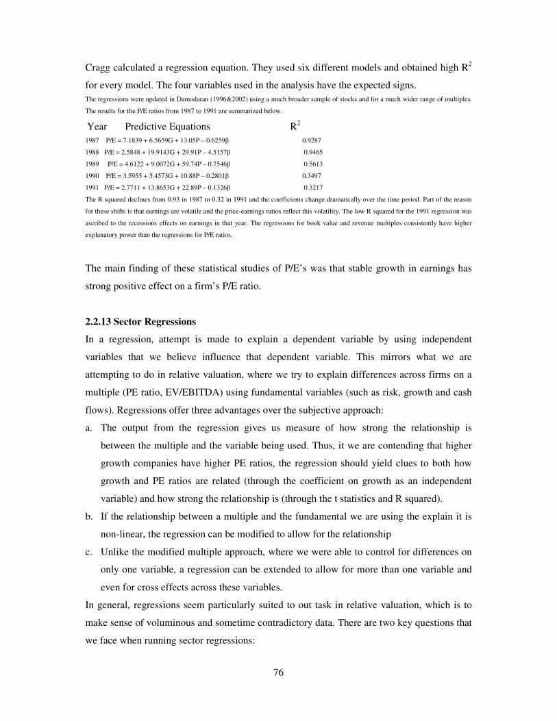
76
Cragg calculated a regression equation. They used six different models and obtained high R2
for every model. The four variables used in the analysis have the expected signs.
The regressions were updated in Damodaran (1996&2002) using a much broader sample of stocks and for a much wider range of multiples.
The results for the P/E ratios from 1987 to 1991 are summarized below.
Year Predictive Equations R2
1987 P/E = 7.1839 + 6.5659G + 13.05P – 0.6259� 0.9287
1988 P/E = 2.5848 + 19.9143G + 29.91P – 4.5157� 0.9465
1989 P/E = 4.6122 + 9.0072G + 59.74P – 0.7546� 0.5613
1990 P/E = 3.5955 + 5.4573G + 10.88P – 0.2801� 0.3497
1991 P/E = 2.7711 + 13.8653G + 22.89P – 0.1326� 0.3217
The R squared declines from 0.93 in 1987 to 0.32 in 1991 and the coefficients change dramatically over the time period. Part of the reason
for these shifts is that earnings are volatile and the price-earnings ratios reflect this volatility. The low R squared for the 1991 regression was
ascribed to the recessions effects on earnings in that year. The regressions for book value and revenue multiples consistently have higher
explanatory power than the regressions for P/E ratios.
The main finding of these statistical studies of P/E’s was that stable growth in earnings has
strong positive effect on a firm’s P/E ratio.
2.2.13 Sector Regressions
In a regression, attempt is made to explain a dependent variable by using independent
variables that we believe influence that dependent variable. This mirrors what we are
attempting to do in relative valuation, where we try to explain differences across firms on a
multiple (PE ratio, EV/EBITDA) using fundamental variables (such as risk, growth and cash
flows). Regressions offer three advantages over the subjective approach:
a. The output from the regression gives us measure of how strong the relationship is
between the multiple and the variable being used. Thus, it we are contending that higher
growth companies have higher PE ratios, the regression should yield clues to both how
growth and PE ratios are related (through the coefficient on growth as an independent
variable) and how strong the relationship is (through the t statistics and R squared).
b. If the relationship between a multiple and the fundamental we are using the explain it is
non-linear, the regression can be modified to allow for the relationship
c. Unlike the modified multiple approach, where we were able to control for differences on
only one variable, a regression can be extended to allow for more than one variable and
even for cross effects across these variables.
In general, regressions seem particularly suited to out task in relative valuation, which is to
make sense of voluminous and sometime contradictory data. There are two key questions that
we face when running sector regressions:

77
• The first relates to how we define the sector. If we define sectors too narrowly, we run the
risk of having sample sizes, which undercut the usefulness of the regression. Defining
sectors broadly entails fewer risks. While there may be large differences across firms
when we do this, we can control for those differences in the regression
• The second involves the independent variables that we use in the regression. While the
focus in statistics exercises is increasing the explanatory power of the regression (through
the R – squared) and including any variables that accomplish this, the focus of regressions
in relative valuations is narrower. Since our objective is not to explain away all
differences in pricing across firms but only those variables that are related to those
fundamentals. As an example, consider the PE ratio. Since it is determined by the payout
ratio, expected growth and risk, we should include only those variables in the regressing.
We should not add other variables to this regression, even if doing so increase the
explanatory power, if there is no fundamental reason why these variables should be
related to PE ratios.
2.2.14 Market Regression
Searching for comparable firms within the sector in which a firm operates is fairly restrictive,
especially when there are relatively few firms in the sector or when a firm operates in more
than one sector. Since the definition of a comparable firm is not one that is in the same
business but one that has same growth, risk and cash flow characteristics as the firm being
analyzed, we need not restrict our choice of comparable firms to those in the same industry.
The regression introduction in the previous section controls for differences on those variables
that we believe cause multiples to vary across firms. Based upon the variables that determine
each multiple, we should be able to regress PE, PBV and PS ratios against the variables that
should affect them. It is however, possible that the proxies that we use for risk (beta), growth
(expected growth rate in earnings per share), and cash flow (payout) are imperfect and that
the relationship is not linear. To deal with these limitations, we add more variables to the
regression e.g. the size of the firm may operate as a good proxy for risk.
The first advantage of this market-wide approach over the “subjective” comparison across
firms in the same sector, described in the previous section, is that it does quantify, based upon
actual market data, the degree to which higher growth or risk errors are a reflection of the
reality that many analysts choose not to face when they make subjective judgments. Second,
by looking at all firms in the market, this approach allows us to market more meaningful

78
comparisons of firm that operate in industries with relatively few firm. Third, it allows us to
examine whether all firms in an industry are under or overvalued by estimating their value
relative to other firms in the market.
2.2.15 Estimation of the Fundamentals
2.2.15.1 Estimation of Beta Coefficient (�)
Past security returns constitute the data base most frequently used to estimate beta(Akintola-
Bello 2004:139). The number of observations and time interval used in the regression vary.
For instance, Value-Line Investment Services used weekly rates of return for the most recent
5 year(260 weekly observations). Merrill Lynch, a U.S investment firm, used the most recent
60 monthly observations to estimate beta for U.S firms on the New York Stock Exchange
(NYSE). Similarly, the London Business School Risk Measurement Service used 60 most
recent months observation to estimate beta for UK firms quoted on the London Stock
Exchange. Several studies by Statman (1981) and Redly-Wright (1988) that examined the
relationship between value line and Merrill Lynch betas found a weak relationship. Akintola-
Bello (2004:139) used 96 months of security returns from Jan 1992 to December 1999 to
estimate the betas for 173 firms quoted on the Nigerian stock exchange. He used growth rates
in the NSE All-share index as the proxy for the market rate of return.
It is generally accepted that due to some statistical factors, the estimated betas using the
regression analysis are not unbiased estimates of the underlying beta of a firm’s securities.
The underlying beta of a security is likely to be closer to 1 than the sample estimate. To
correct, for this bias, Merrill Lynch developed an adjustment technique. After using the
ordinary least squares to gain a preliminary estimate of beta, using 60 monthly returns, the
beta is adjusted as follows:
Adjusted Beta = 2/3(Computed Sample Beta) + 1/3(1)
= 0.67(Raw beta) + 0.33(1)
The formula pushes high betas down toward 1.0 and low betas up toward 1.0. The raw betas
computed are adjusted to remove individual’s securities bias.
Therefore, the conventional approach for estimating betas used by most investment firms,
analysts and services is to use historical market data for firms that have been quoted for a
long period. One can estimate returns that an investor would have made on their investments
in intervals (such as a week, a month) over that period. These returns can then be related to a
proxy for the market portfolio to get a beta that will be used in the CAPM.

79
The Beta (�) can be used in the following applications:
(1)to determine the expected rate of return for a risky asset, via Ri = Rf + �(Rm – Rf), (2)to
determine the cost of equity capital, via Ke = Rf + �(Rm – Rf), (3) to determine the portfolio
risk via Portfolio Beta = �p = �Wi �i, (4) to classify stocks into Aggressive stocks(or High
Beta stocks) with � of 1.06-1.79, Conservative stocks(or average beta stocks) with � of 0.93-
1.05, Defensive stocks(or low beta stocks) with � = 0.02-0.92
In the fourth beta application, recall that the return on any security varies with the security’s
beta. Beta measures the sensitivity of a stock’s return to changes in the return on the market
or the index. That is, beta measures the sensitivity of the underlying assets prospects and
investor’s assessment thereof to those of the economy as a whole. Beta indicates how a stock
is expected to move, up or down, relative to the overall market. Usually a stock with a higher
beta represents a more volatile and riskier investment.
The beta of the overall stock market is + 1.0 and every other stock beta is viewed in relation
to this value, + 1.0. A stock with beta of exactly one will on the average move by just one
percent for every one percent movement by the market. A stock with a beta of 1.5 tends to be
50% more volatile than the average stock market index, while that with a beta of 0.5 is half as
volatile. If a stock with a beta rating of 1 move 10% another stock with a beta equal to 2 can
be expected to move twice as much (ie. 20%). The beta usually used in stocks classification is
the adjusted stock beta (Akintola 2004:168).
When the stock market is declining, a stock with a beta rating of less than one is preferred.
The reason is that such a stock is expected to decline less than the market. Conversely, in a
rising market, such a stock will underperform compared to the overall market. When the
overall market is rising, a stock with a high beta is expected to out-perform the market. An
investor’s objective during the stock selection process is to identify stocks that will (1) Rise
faster than the average stock during a bull market (2) Decline less than the average stock
during a bear market.
2.2.15.2The Capital Assets Pricing Model (CAPM)
The CAPM was developed by Sharpe (1964) John Lintner (1965), Mossin (1966) in an
attempt to simplify the individual portfolio theory as it relates to investment in securities. It

80
states that the return on any asset or portfolio is related to the riskless rate of return and the
expected return on the market in a linear fashion. It shows the relationship between expected
return of a security and its unavoidable systematic risk thus, R = Rf + �(Rm – Rf)
Where
R = Expected rate of return on a security or a portfolio
Rf = Risk-free rate of return
Rm = Expected market rate of return �� ��
= Systemic risk of the security (the beta) relative to that of the market.
The model submits that only risk which cannot be diversified away, i.e. systemic risk, is
worthy of being rewarded with a risk premium for financial valuation purposes. The
remaining risk, i.e. unsystemic or diversifiable risk may be reduced to zero by portfolio
diversification and so it is not worthy of a risk premium. The line that reflects the
combination of systemic risk and return available on alternative investments at a given time is
called the security market line (SML). Any security that lies on the SML is being correctly
priced. If there is temporary disequilibrium in the market and the return on some assets
becomes higher than that given by the SML, then the security is underpriced. Under this
market condition, if the market mechanism is working ideally, as investors demand more of
such securities as super-good investment, the prices will continue to rise until that higher
level of return reaches the SML value. Conversely if as a result of the market disequilibrium
the level of return is lower than that given by the SML, then the security is overpriced. Under
this market condition, if the market mechanism is working ideally, as investors sell-off more
of such securities as super-bad investment, the prices will continue to fall until the level of
return rises to that given by the SML value. Therefore, investors should select investments
that are consistent with their risk preferences. While some investors consider only low risk
investments, others welcome high risk investments. However, investors should sell
overpriced securities, buy underpriced securities, and hold onto correctly priced securities.
The key to this decision is that when
actual return –CAPM required return = +ve alpha, the security is underpriced,
actual return –CAPM required return = zero alpha, the security is correctly priced,
actual return –CAPM required return = -ve alpha, the security is overpriced
The CAPM provides a framework for valuation of securities.
Return
SML
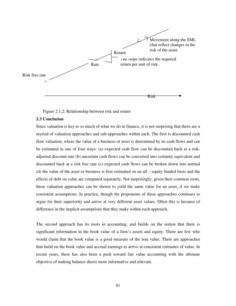
81
Movement along the SML chat reflect changes in the risk of the asset.
2
Risk
Figure 2.1.2: Relationship between risk and return
2.3 Conclusion
Since valuation is key to so much of what we do in finance, it is not surprising that there are a
myriad of valuation approaches and sub-approaches within each. The first is discounted cash
flow valuation, where the value of a business or asset is determined by its cash flows and can
be estimated in one of four ways: (a) expected cash flow can be discounted back at a risk-
adjusted discount rate (b) uncertain cash flows can be converted into certainty equivalent and
discounted back at a risk free rate (c) expected cash flows can be broken down into normal
(d) the value of the asset or business is first estimated on an all – equity funded basis and the
effects of debt on value are computed separately. Not surprisingly, given their common roots,
these valuation approaches can be shown to yield the same value for an asset, if we make
consistent assumptions. In practice, though the proponents of these approaches continues to
argue for their superiority and arrive at very different asset values. Often this is because of
difference in the implicit assumptions that they make within each approach.
The second approach has its roots in accounting, and builds on the notion that there is
significant information in the book value of a firm’s assets and equity. There are few who
would claim that the book value is a good measure of the true value. There are approaches
that build on the book value and accrual earnings to arrive at consistent estimates of value. In
recent years, there has also been a push toward fair value accounting with the ultimate
objective of making balance sheets more informative and relevant.
The slope indicates the required return per unit of risk.
Return
Rate
Risk free rate

82
The third approach to valuation is relative valuation, where we value an asset based upon
how similar assets are priced. It is built on the assumption that the market, while it may be
wrong in how it prices individual assets, gets it right on average and is clearly the dominant
valuation approach in practice. Relative valuation is built on standardized prices, where we
scale the market value to some common measure such as earnings, book value or revenues,
but the determinants of these multiples are the same ones that underlie discounted cash flow
valuation.
In the DCF valuation attempt is made to estimate the intrinsic value of an asset based upon its
capacity to generate cash flows in the future. In the relative valuation attempt is made to
make a judgment on how much an asset is worth by looking at what the market is paying for
similar assets. If the market is current, on overage, in the way it prices assets, the DCF and
relative valuations may converge. If the market is systematically over pricing a group of
assets or an entire sector, DCF valuations can deviate from relative valuations.
The DCF valuation has been a search for intrinsic value. In relative valuation, intrinsic value
estimation is abandoned and trust put in markets getting it right, at least on average.
Damodran (2002) notes 550% of acquisition valuations use some combination of multiples
and comparable companies and these are relative valuations. It can be argued that most
valuations are relative valuations.

83
References
Akintola-Bello, O. (2005), “How common stocks are valued,” The Nigerian Stockbroker Vol.6 No.2 April – June 2005, 3 – 11.
Akintola-Bello, O. (2004), “The Nigerian Stock Market: Behaviour and Performance”, Lagos, Arbitrage consulting group.
Akintola-Bello, O. (1990), “De-mystifying the P/E Ratio” Stock Guide, Vol.2, No.1 September, Arbitrage Consulting Group, 25 – 29.
Akintola-Bello, O. (1989), “The Riddle of Price-Earnings Ratio,” Stock Guide, April/May, Arbitrage Consulting Group, 49-51. Alford, A.W. (1992), ‘The Effect of the set of Comparable Firms on the Accuracy of the Price- Earnings valuation Method,’ Journal of Accounting Research Vol 30, 94 – 108.
Amedu, S. (2004), “Investing in shares/stocks and other options in Nigeria” The Nigerian Stockbroker, Vol.5 No.3, July-September 2004, 22-31.
Andrade, G. and Kaplan, S. (1998), ‘How costly is financial (not Economic) Distress? Evidence from Highly Leveraged Transactions that became distressed’ Journal of Finance 53, 14443 – 493.
Baker, M. and Wurgler, J. (2004a), ‘Appearing and Disappearing Dividends: the Link to Catering incentives’ Journal of Financial Economics 73, 271-288. Baker, M. and Wurgler, J. (2004b), ‘A catering theory of Dividends’ Journal of Finance 59, 1125-1165.
84
Barth, M. E. (1994), Fair Value Accounting: Evidence from Investment Securities and the Market Valuation of Banks’ Accounting Review Vol 69.No 1 (January): 1 – 25. Barth, M. E.; Landsman, W. R. and Whalen, J. M. (1995), ‘ Fair value Accounting: Effects on banks’ earnings volatility, regulatory capital, and value of contractual cash flows’ Journal of Banking and Finance vol 19, No 3 – 4 (June): 577 -605.
Barth, M. E.; Beaver, W. and Landsman, W. (2001), ‘The Relevance of the Value Relevance literature for financial Accounting standard setting: Another View’ Journal of Accounting and Economics 31, 77 – 104.
Barth, M. E.; Beaver, W. H. and Landsman, W. R. (1996), ‘Value relevance of banks fair value disclosures under SFAS 107’ The Accounting Review, vol.71 No. 4 (October), 513 – 537.
Barth, M. E. and Uinch, G. (1998), ‘Revalued Financial, Tangible and intangible assets: Associations with share price and non-market-based value estimates’ Journal of Accounting Research Vol 36 (Supplement), 199-233.
Beatty, R. P.; Riffe, S. M. and Thompson, R. (1999), ‘The Method of comparables and tax court valuations of private firms: An empirical Investigation” Accounting Horizons 13, 77 – 199.
Beaver, W. and Merse, D. (1978), ‘What do P/e ratios Means? Financial Analysts Journal, vol 34, 65– 76.
Beedles, W.L. ( 1̀978), ‘Evaluation of Negative Benefits’ Journal of Financial and Quantitative Analysis Vol. 13, 173 – 176.
Benjamin, G. (1951), ‘Securities Analysis’, Columbia University Press, 389.
Benjamin, G. (1949), ‘The Intelligent Investor’, Harper Collins.
Berger, P.; Ofek, E. and Swary, I. (1996), ‘Investor Valuation of the Abandonment Option’ Journal of Financial Economics Vol 42, 257 – 287.
Berkman, H.; Bradbury, M. E. and Ferguson, J. (2000), The Accuracy of Price Earnings and Discounted Cash Flow Methods of IPO Equity Valuation, Journal of International Financial Management and Accounting, Vol 11, 71 – 83.
Bhojraj, S. and Lee, C. M. C. (2002), ‘Who is my peer? A valuation – based approach to the Selection of comparable firms’ Journal of Accounting Research, Vol 40, 407 – 439.
85
Bhojraj, S.; Lee, C. M. C., and Oler, D. (2003), ‘What’s my line? A comparison of industry classification schemes for capital Market Research’ Journal of Accounting Research, Vol 41, 745 – 774.
Boatman, J. R. and Baskin, E. F. (1981), ‘Asset Valuation in Incomplete Markets’ Accounting Review, 38 – 53.
Bohm-Bawerk, A. V. (1903), “Recent Literature on Interest” Macmillan.
Boulding, K. E. (1935), “The Theory of a Single investment”, Quarterly Journal of Economics, Vol. 49, 479 – 494.
Bower, R.S. and Bower, D.H. (1969), “Risk and the Evaluation of Common Stocks” Journal of Political Economy, May-June, 349-362. Brealey, R. A. and Myers, S. E. (2003), ‘Principles of Corporate Finance’, 7ed, McGraw-Hill Irwin.
Brealey, R. A. (2004), ‘Investment Valuation’, 3ed, New York, John Wiley.
Buchanam, D. (2000), ‘Business Valuators Must Dig Behind the Hype’ Washington Business Journal, September 15.
Cheng, C. S. A. and McNamara, R. (2000), ‘The Valuation Accuracy of the Price earnings and price-book benchmark valuation Methods, Review of Quantitative finance and Accounting Vol 15, 349 – 370.
Chen, C.; Kohlbeck, M. and Warfield, T. (2004), “Goodwill Valuation Effects of the Initial Adoption of Sfas 142, Working Paper, University of Wisconsin-Madison.
Chinyere, J. (2007), ‘NASCON Should Go for Hybrid Offer’ Stock Watch, May 27, 2007, p.5
Cohen, J. B.; Zinbrag, E. D.; and Zeikel, A. (1977), “Investment Analysis and Portfolio Management”, Homewood, III R.D. Irivin, pp 245-255.
Cooper, I. A. and Nyborg, K. G. (2006), ‘The value of tax shields is equal to the present value of the Tax shields,’ Journal of Financial Economics, Vol. 81, 215-225.
Copeland, T.E.; Koller T. and Murrin, J. (1990), ‘Valuatio: Measuring and Managing the Value of companies’ John Wiley and Sons.
Courteau, L.’; Kao, J. and Richardson J. (2001), ‘The Equivalence of Dividend, cashflow Equity Valuation Employing ideal Terminal value Calculations’ Contemporary Accounting
86
Research Vol 18, 625-661.
Damodaran, A. (2006), ‘Valuation Approaches and Metrics: A Survey of the Theory and Evidence’ Stern School of Business, November, pp 1-77.
Damodaran, A. (2006), ‘Darnodaran on valuation’ 2ed, York, John Wiley.
Damondaran, A. (2002), “Investment Valuation Tools and Techniques for Determining Value”, New York, John Wiley and Sons.
Damodaran, A. (1999), ‘Value Enhancement: Back to Basics’ Contemporary Finance Digest Vol 2, 5-51.
DeAngelo, H.; DeAngelo, L. and Skinner, D. (2004), ‘Are Dividends Disappearing? Dividend concentration and the consolidation of Earnings’ Journal of Financial Economics Vol 72, 425-456.
Dechow, P.; Hutton, A. and Slan, R. (1999), ‘An Empirical Assessment of the Residual income valuation model” Journal of Accounting and Economics 26 (1 – 3) – 34.
Dodd, D. and Graham, B. (1934), ‘Security Analysis’ New York, McGraw Hill.
Durand, D. (1957), ‘Growth Stocks and the St Petersburg Paradox’ Journal of Finance, vol.12, 348-363.
Easton, P. (2004), ‘Pe Ratios, PEG Ratios and Estimating the Implied Expected Rate of Return on Equity capital’ The Accounting Review, Vol 79, 79-95.
Edwards, E. and Bell, P. (1961), “The theory and management of Business Income”, Berkley, University of California press.
Fairfield, P. (1994), “P/E, P/B and the present value of future dividends” Financial Analysts Journal, Vol 50, 23 – 31.
Fama, E. F. and French, K. R. (1992), ‘The cross-section of Expected Returns’ Journal Of Finance Vol. 47, 427 – 466.
Felthan, G. and Ohlson, J. (1995), ‘Valuating and Clean Surplus Accounting of Operation and Financial Activities”, Contemporary Accounting Research, Vol 11, 689-731.
Fernandez P. (2004), ‘Equivalence of 10 different discounted cash flow valuation methods’ IESE Research papers, D549.
87
Fernandez, P. (2002), ‘Three Residual Income Valuation Models and Discounted cash flow Valuation Working Paper, IESE Business School. Fisher, I. (1930), ‘The Theory of Interest’ New York, Macmillan. Fisher, I. (1907), ‘The Rate of Interest’ New York, Macmillan. Francis, J.; Olsson, P. and Oswaled, D. (2000), ‘Comparing the Accuracy and Explain ability Of Dividend, Free cash Flow and Abnormal Earnings Equity Value Estimates’ Journal of Accounting Research Vol 38, 45-70. Frankel, R. and Lee, C. M. C. (1998), ‘Accounting valuation, market Expectations, and cross-sectional stock Returns’ Journal of Accounting Economics, Vol 25, 283 – 319. Fuller, R. J. and Hisa, C. (1984), ‘A Simplified Common Stock Valuation Model’, Financial Analysis Journal Vol.40, September/October, 49-56. Gilson, S. C.; Hotchkiss, E. S. and Ruback, R. S. (1998) ‘Valuation of Bankrupt firms’ Review of Financial Studies Vol 13, 43 -74.
Goedhart, M.; Koller, T.; Mickinsey, C. and Wessels, D. (2005), Valuation Measuring and Managing the value of companies” John Wiley. Gordon, M. J. (1962), “The Investment Financing and Valuation of the Corporation, Homewood 111, Richard D. Irwin. Gregory, D. D. (1978), ‘Multiplicative Risk Premiums,’ Journal of Financial and Quantitative Analysis vol 13, 947-963.
Hagstron, R. (2004), ‘The Warren Buffett Way,’ New York, John Wiley.
Hand, J. R. M. and Landsman, W. R. (1999), ‘Testing the Ohlson Model: v or not, that is the question, working paper, university of North Carolina Chapel Hill.
Hartman, J. C. (2000), “On the Equivalence of Net Present Value and Economic Value Added as measures of a project’s Economic worth” The Engineering Economist Vol 45, 158 -165.
Hoberg, G. and Prabhala, M. R. (2005), ‘Disappearing Dividends: the importance of Idiosyncratic risk and the Irrelevance of Catering,’ Working Paper” University of Maryland.
Holland, M. (1990), ‘When the machine Stopped’, Harvard Business School press, Cambridge, MA.
Holthanusen, R. and Watts, R. (2001), ‘the Relevance of the value –Relevance Literature for financial Accounting standard setting’ Journal of Accounting and Economics, Vol 31, 3-75.

88
Howe, J. S.; Kim, S.’; Lee, E. (1995), “The after market performance of initial public offerings (IPOs): The Korean Experience” Advance in Pacifi-Basin Financial Markets Forthcoming (JAI Press). Inselbag, I. and Kaufold, H. (1997), ‘Two DCF Approaches for valuing companies under alternative Financing strategies and how to choose between them’ Journal of Applied corporate Finance, Vol 10, 114 – 122.
Johansen, J. A. (2000), ‘How To Buy or Sell a Business’ Small Business Administration.
John-Burr, W. (1938), ‘The theory of Investment value’, Harvard University Press, p.89.
Kane, A.; Marcus, A. J. and Noh, J. (1996), ‘The P/E Multiple and market Volatility’ Financial Analysts Journal vol 52, 16 – 24.
Kaplan, S. N. (1987), “Campeau’s Acquisition of Federated: Value Destroyed or Value Added? Journal of Financial Economics Vol 25, 191 – 212.
Kaplan, S. N., Ruback, R. S. (1995), “The Valuation of Cash Flow Forecasts: An Empirical Analysis”, Journal of Finance, Vol 50, 1059 – 1094.
Keck, T.; Levengood, E.; Longfield, A. (1998), ‘Using Discounted Cash Flow Analysis in an international setting: A survey of Issues in modeling the cost of capital’, Journal of Applied Corporate finance, fall, 82- 99.
Keynes, J. M. (1936), “The General Theory of Employment” London, Macmillan. Koller, T.’; Goedhart, M. and Wessels, D. (2005) Valuation; Measuring and Managing the value of companies’ 4ed, John Wiley. Kim, J.; Krinsky, I.; Lee J. (1995b), ‘The aftermarket performance of initial public offering in korea’, Pacific-Basin finance Journal (Forthcoming).
Kim, J.; Krinsky, I.; Lee, J. (1995), ‘The Role of Financial variables in the pricing of Korean Initial Public Offerings’ Pacific-Basin Finance Journal 3, 449-464.
Kim, J., Kinsky, I. (1993), ‘Motives for going public and under-pricing: New findings from Korea, Journal of Business Finance and Accounting, 195 – 211. Kim, M. and Ritter, J. R. (1999): Valuing Impose, Journal of Financial Economics,Vol 53, 409 – 437.

89
Lang, L. H. P.; Stulz, R. M. and Walking, R. (1989), “Management Performance, Tobin’s Q, and the Gains from Successful Tender Offers “Journal of Financial Economics Vol 29, 137-154.
Lee, C. M. C.; Myers, J. and Swaminathan, B. (1999), What is the intrinsic value of the Dow?, Journal of Finance, Vol 54, 1693 – 1741.
Leibowitz, M. L. and Kegelman, S. (1992), ‘Franchise value and the Growth factor’ Financial Analysts Journal, Vol 48, 16 – 23.
Leibowitz, M. L. and Kegelman, S. (1991), “The franchise Factor for leveraged Firms’’ Financial Analysts Journal Vol 47, 29 – 43.
Leibowitz, M. L. and Kegelman, S. (1990), ‘Inside the PE ratio: the Franchise Factor’
Financial Analysts Journal Vol 46, 17 – 35
Leibowitz, M. L. (1997), ‘Franchise Margins and the Sales -Driven Franchise Value. Financial Analysts Journal Vol 53, 43 – 53.
Lev, B. (1989), ‘On the usefulness of Earnings: Lessons and directions from two decades of empirical Research’ Journal of Accounting Research Vol 27 (Supplement): 153 -192. Lie, E. and Lie, H. J. (2002), ‘Multiples used to Estimate corporate value’ Financial Analysts Journal Vol 58, 44 – 54 Liu, J.; Nissim, D.; and Thomas, J. (2002), ‘Equity valuation using Multiples” Journal of Accounting Research, Vol 40, 135 – 172.
Lo, K. and Lys, T. (2005), ‘The Ohlson model: Contribution to Valuation Theory, Limitations and Empirical Applications, working Paper Kellogg School of Management North western University.
Luehrman, T. A. (1997),’Using APV: A better Tool for valuing Operations’ Harvard Business Review, May – June, 145 – 154. Lundhalm, R. and Okeefe, T. (2001), ‘Reconciling value estimates from the Discounted cash Flow model and the residual income model”, Contemporary Accounting Research vol 18, 311- 335. Madden, B. L. (1998), ‘CFROI cash flow Return on Investment Valuation: A Total System Approach to Valuing a firm’ Butter worth Heinemann.
Malkiel, S. and Cragg, R. (1970), ‘The effects of historical growth of earnings, dividend payout, and the stock’s rate of return relative to the market in determining P/E’ Proponents’ Journal of Applied Finance, Full/Winter, 7-17.
90
Mao, J. C. T. (1974), ‘Valuation of Growth stocks: the investment Opportunities Approach’ Journal Of finance, Vol 21, 95 – 102. Marshal, A. (1907), “Principles of Economics, Macmillan. Medaglia, A. (1999), ‘Corporate Valuation: Is There Room For Improvement?” Fordham Business Review, January. Michaud, R. O. and Davis, P. L. (1981), “Valuation model Bias and the scale structure of dividend discount returns’ Journal of Finance, vol 37, 563-573. Miles, J. and Ezzell, J. R. (1980), ‘The Weighted Average cost of Capital, Perfect capital Markets and project life: A clarification’ Journal of Financial and Quantitative Analysis Vol 40, 1485-1492. Miller, M. H. and Modigliani, F. (1963), ‘Corporate Income Taxes and the cost of capital: A Correction’ American Economic Review Vol 53, 433– 443. Miller, M. H. and Modigliani, F. (1958), ‘The cost of Capital, Corporation Finance and the Theory of Investment’ American Economic Review Vol 48, 261– 297. Moonchul, K.; Ritter J. R. (1999), ‘Valuing IPOs’ Journal of Financial Economics, Vol 53 No.3, September, pp409-437. Myers, S. (1974), ‘Interactions in corporate Financing and investment Decisions Implications for Capital Budgeting’ Journal of Finance Vol 29,1-25.
Nelson, K. K. (1996), ‘Fair value Accounting for commercial Banks: An Empirical Analysis of SFAS 107’ The Accounting Review Vol 71,161-182. Ohlson, J. (1995), ‘Earnings, Book Values and Dividends in Security Valuation Contemporary Accounting Research, Vol 11, 661-687. Olusoji, O. O. (2004), ‘Valuation of Securities – Risk and Return’ The Nigerian Stockbroker, July-September, Volume 5 No.3, 11-21. Oper, T. and Tilman, S. (1994), ‘Financial Distress and corporate Performance’ Journal of finance 49, 1015 – 1040. Parker, R. H. (1968), ‘Discounted Cash Flow in Historical Perspective’ Journal of Accounting Research, Vol. 6, 58 – 71 Peasnell, K. (1982), ‘Some Financial connections between Economic Values and Accounting Numbers’ Journal of Business Finance and Accounting Vol 9, 361 – 381. Penman, S. H. (1998), ‘A Synthesis of Equity Valuation Techniques and the Terminal value Calculation for the Dividend Discount Model (DDM)’ Review of Accounting Studies, Vol 2, 303 – 323.

91
Penman , S. H. (1996), ‘The Articulation of price – Earnings and market – to – Book Ratios and the Evaluation of Growth’ Journal of Accounting Research Vol. 34, 235 – 259. Penman, S. and Sourgiannis (1998), ‘A Comparison of Dividend, Cash flow, and Earrings Approaches to Equity Valuation’ Contemporary Accounting Research, Vol 15, 343 – 383. Penman S. and Sourgiannis (1997), ‘The Dividend displacement Property and the Substitution of Anticipated Earnings for Dividends in Equity Valuation” The Accounting Review Vol 72, 1-2. Pennel, W. O. (1914), ‘Present worth Calculation in Engineering Studies” Journal of the Association of Engineering Societies. Robber, F. W. (1930), ‘Investing for future values’ Baron’s, September 8, p.5 Robichek, A. A. and Myers, S. C. (1966), “Conceptual Problem in the Risk-Adjusted Discount Rates” Journal of Finance, Vol 21, 727-730. Ruback, R. S. (2000), ‘Capital cash flows: A simple Approach of valuing Risky cashflows’ working Paper, Harvard Business School. Ruback, R. S. (1995), ‘An introduction to cash flow Valuation methods’ Harvard Business school case No. 295 – 155. Samuelson, P. (1937), “Some Aspects of the pure theory of capital” Quarterly Journal of Economics, Vol 51, 469 – 496. Shleifer, A. and Vishny, R. W. (1992), ‘Liquidation Values and Debt Capacity: A market Equilibrium Approach,’ Journal of Finance, Vol 47, 143 – 166. Shrieves, R. E. and Wachowicz, J. M. (2000), “Free Cash Flow, Economic Value Added and Net Present Value: A Reconciliation of Variations of Discounted Cash Flow Valuation, Working Paper, University of Tennessee. Stapleton, R. C. (1971), ‘Portfolio Analysis, Stock Valuation and Capital Budgeting Decision Rules for Risky Project’ Journal of Finance Vol 26, 95 – 117. Stewart, G. B. (1991), ‘The Quest for Value: The EVA management Guide, Harper Business. Slee, R. (1999), ‘How Much is Your Small Business Worth to a Roll-Up? Triangle Business Journal, August 20. Terry, J. W. and Keith, P. (2007), ‘Quantitative Methods in Finance’ 5ed, United Kingdom, Thomson. Tuller L. W. (1990), ‘Getting Out: A Step-by step Guide to Selling a Business or Professional Practice, Liberty Hall. Varaiya, N.; Bergmark, B.; Taylor, R., (1997), ‘F&C International: A case of an IPO Valuation’ Journal of Financial Education 23, 114 – 123.

92
Walter, J. E. (1966), ‘Dividend Policies and Common stock pries, Journal of Finance Vol 11, 29 – 41. Warner, J. N. (1977), ‘Bankruptcy costs: some Evidence ‘Journal of finance, vol 32, 337 – 347. Weaver, S. C. (2001), ‘Measuring Economic Value Added; A Surevey of the Practices of EVA Proponents’ Journal of Applied Finance Full / Winter, 7 – 17. Wellington, A. M. (1887), “The Economic Theory of the Location of Railways” New York, Wiley. Wilcox, J. (1984), ‘The P/B – ROE Valuation model’ Financial Analysts Journal 58-66 Williams, J.B. (1938), ‘The Theory of Investment Value’, Cambridge MA, Harvard University Press. Williamson, O. E. (1988), ‘Corporate Finance and corporate Governance’ Journal of Finance, Vol 43, 567 – 592. Whitbeck, V. S. and Kisor, M. (1963), ‘A New Tool in Investment Decision Making’ Financial Analysts Journal, May-June, pp. 52-62. Yegge, W. M. (1996), ‘A Basic Guide to Buying and Selling a company, John Wiley. Young S.D. and OByrne (2000), ‘EVA and Value Based Management’ McGraw-Hill. Zarowin P. (1990), ‘What determines earnings – price ratios: Revisited’ Journal of Accounting, Auditing and Finance, Vol 5, 439 – 457.

93
CHAPTER THREE
RESEARCH METHODOLOGY
3.0 Introduction
The methodology adopted for any research is of utmost importance because the reliability
and acceptability, or otherwise, of the study depends to a large extent on it. This is because
the research method provides the background against which a reader evaluates the findings
and conclusions drawn from the study. This is much more important and pertinent in our
study which relied mainly on data collected from the Nigerian Stock Exchange with its
peculiarities. It is expected that whatever model is adopted in the study, should not only be
appropriate but should also be able to accommodate such peculiarities characteristic of the
Nigerian Stock Exchange. Thus, in this chapter we present a detailed explanation of the
research methods adopted for this study. It also reveals the methods of data collection,
organization, analyses, summarization, and presentation.
3.1 Theoretical Framework for the Study
There are three approaches to equity share valuation namely the DCF valuation, accounting
valuation, and the relative valuation. The differences in value among the three come from
different views of market efficiency or inefficiency. In DCF valuation, we assume that
markets make mistakes, that they correct these mistakes over time, and that these mistakes
can often occur across entire sectors or even the entire market. In DCF, the value of a
94
business or asset is determined by its cash flows in one of four ways: (i) expected cash flows
can be discounted back at a risk-adjusted discount rate, (ii) uncertain cash flows can be
converted into certainty equivalents and discounted back at a risk-free rate, (iii) expected cash
flows can be broken down into normal(representing a fair return on capital invested) and
excess return cash flows and valued separately, (iv) the value of the asset or business is first
estimated on an all-equity funded basis and the effects of debt on value are computed
separately. The accounting valuation builds on the notion that there is significant information
in the book value of a firm’s assets and equity. In relative valuation, we assume that while
markets may make mistakes on how they price individual stocks, they are correct on average.
Here we value an asset based upon how similar assets are priced. Relative valuation is built
on standardized prices upon which market value is scaled to some common measure such as
earnings, book value or revenues. It is the dominant valuation approach in practice. Based on
this line of thought and the availability of data, two relative valuation methods namely the
Capital Asset Pricing Model(CAPM) developed by Sharpe(1964) and the Kisor and
Whitbeck Model(KWM) developed by Kisor and Whitbeck(1963) are adopted in this study.
3.2 Research Design
Research design is the plan, structure and strategy of investigation conceived to accomplish a
research work. This research is on valuation and pricing of equity securities in the Nigerian
stock market using empirical evidence from banking sector. The problem the study sets out to
address is that there seems to be no clear cut method of fixing share prices in the market.As
has been shown in chapter one, the major objective of this study is to examine the adequacy
of some of the models that guide stock price movement in most of the earlier research works
using data from the developed markets, in emerging stock markets such as the Nigerian Stock
Exchange. It is also not clear whether the efficient market hypothesis has a place in the
pricing mechanism of the market. In the light of the above assertion, the objective of this
study is to find out the model that best describes the pricing of ordinary shares in Nigerian
stock market with special interest in banking stocks. The decision to research only on
banking stocks is informed by the fact that banks are the major financier of other sectors and
hence banking stock prices should influence the price of stocks in other sectors. The study
will display the level of the market prices to the intrinsic values of the subject companies’
shares.
95
Being an empirical study, analytical research design is adopted. The data used are secondary
data, which are collected from the financial statements of the banks, The Nigerian Stock
Exchange publications, and Central Banks of Nigeria (CBN) publications. In line with
previous similar studies on securities valuation, the Capital Asset Pricing Model (CAPM) and
the Kisor and Whitbeck Model (KWM) will be employed to determine the required rates of
return and the P/E multiples of the equity securities.
In the relative valuation, an asset is valued based upon how similar assets are priced in the
market. That is, an asset worth is determined by looking at what the market is paying for
similar assets. Relative valuation is built on standardized prices, where we scale the market
value to some common measure such as earnings, book value or revenues. Again, relative
valuation is built on the assumption that the market, while it may be wrong on how it prices
individual assets, gets it right on average and is clearly the dominant valuation approach in
practice(Malkiel and Cragg 1970; Bing 1971; Cohen and Zinbarg 1977; Fischer and Jordan
1995; Akintola-Bello 2004; Damodaran 2006).
3.3 Nature and Sources of Data
Data for this study are of secondary nature. To compute the monthly average prices for 96
months (2000 – 2007) the daily market prices of each of the subject banks’ ordinary shares
from 2000-2007 are required. To compute the rates of returns of the subject banks the
following data are required: the Dividends of the subject banks from 2000-2007, the rates of
equity price appreciation or depreciation of the subject banks from 2000-2007, the earnings
of the subject banks from 2000-2007, the growth rates in earnings of the subject banks from
2000-2007, etc. To compute actual and normal P/E ratios of the subject banks using the
relative valuation techniques the following data are required: the price-earnings multiples,
return on assets, return on equity, dividend yields, of the subject banks from 2000-2007.
Therefore, in essence, we need for each subject bank the following data: relevant market
prices, dividends per share history, earnings per share history, earnings growth rates,
dividends growth rates. These data are secondary data that can be derived from the financial
statements of the banks as submitted to the regulatory authorities such as the CBN, SEC and
NSE from 2000-2007. Since these financial statements are audited and published, they
constitute authoritative and official documents to be relied upon in assessing the performance
96
of the affected institutions. The market prices are picked from the NSE daily official list for
2000-2007.
3.4 Population and Sample
In any study, it is important to determine the group of persons or things to study. If the study
contains only part of the group or population, it is referred to as sample(Freund and Williams,
1979). In line with this line of thought, the population for this study is defined as all quoted
banks in the Nigerian Stock Exchange for the period January 2000 to December
2007(Appendix 2). From Appendix 2, out of the 47 banks that were quoted between 2000 and
2007, only 21 banks survived at the end of the bank consolidation exercise that took place
from July 6, 2004 to December 31, 2005. On the whole 25 banks survived the exercise but 4
banks which include Citibank, Equitorial Trust, Stanbic, and Standard Chartered remained
unquoted even after the exercise. Majority of the 47 quoted banks were listed after the
announcement of the consolidation just to enable them to shop for equity funds from the
capital market, in an attempt to increase their bargaining power in consolidating with other
banks. During the consolidation process, many of the banks fused together to produce only 21
quoted banks. When Springbank was excluded from the 21 surviving quoted banks, because
it has not made public any financial statement since its inception and hence there was no
basis to assess its performance, we were left with 20 quoted banks. As a problem bank, it is
still run by the interim management set up by the CBN/NDIC.
The sample for the study is all the quoted banks on the Nigerian Stock Exchange between
years 2000 and 2007. The work was categorized into two periods in order to cover separately
the pre-consolidation era (2000-2005) and post-consolidation era (2006-2007) quoted banks.
In the pre-consolidation era, our sample consists of all the quoted banks from 2000-2005
while in the post-consolidation era, our sample comprises all the quoted banks from 2006-
2007 (appendix 2). Based on these selection criteria, the 23 banks were defined as the sample
for the study for the periods 2000-2005 and 20 banks for the periods 2006-2007, under the
CAPM. Under the Whitbeck-Kisor model, 20 out of the 25 banks and 20 out of the 21 banks
constituted the sample for the 2000-2005 and 2006-2007 respectively, based on the
availability of complete financial records. The sample is the entire population of quoted
banks in Nigeria. We consider the 2000 to 2007 period selected for our study a relatively
stable period in Nigeria as it was fairly free from major political factors that could upturn the
capital market so adversely.
97
3.5 Valuation Methodology
In this study, the required rate of return and the normal P/E of the shares were derived based
upon the Capital Asset Pricing Model (CAPM) and the Whitbeck and Kisor Model (WKM)
respectively. Under the CAPM, the expected required returns as implied by the Capital Asset
Pricing Model (CAPM) were derived and compared with the actual returns from each of the
banks, to ascertain whether the stock was appropriately valued, undervalued, or overvalued,
with respect to the earnings capacity of each of the banks. To accomplish this, it was
necessary to derive value for each of the variables in the equation of the CAPM. Under the
Whitbeck and Kisor Model (WKM), the normal appropriate Price-Earnings ratios were
computed for each of the banks, using a predictive equation that was derived for the banking
industry. The normal P/E ratio was then compared with the actual P/E ratio of each of the
banks to ascertain whether the stock was appropriately value, undervalued, or overvalued. To
accomplish this, it was necessary to derive value for each of the variables in the equation of
the Whitbeck and Kisor Model (WKM).
3.6 Model Specifications
3.6.1 Application of CAPM to Nigerian Banking Industry Data
The Capital Asset Pricing Model (CAPM) was tested on the 23 banks for the period 2000-
2004 and the 20 banks for the period 2005-2007 as categorized above.
3.6.1.1 Estimating the Expected Rate of Return
To adjust for risk the discount rate for each of the banks was determined using the capital
asset pricing model (CAPM) as in Arnold (2008:765). The message of CAPM is that if we
know the risk free rate and the return on the whole market portfolio, the required rate of
return on a risky asset will depend upon its beta coefficient. It tells us that the required rate of
return on an asset is equal to the risk free rate plus a fraction (or multiple) or the market risk
premium, where the fraction (or multiple) is represented by the asset’s beta coefficient. Thus,
Ki = Rf + �i(Rm – Rf)
Where
Ki = cost of equity i, i.e the expected required rate of return
Rf = risk free rate
�i = each equity risk relative to the market
Rm = market rate of return

98
3.6.1.2 Estimating the Risk Free Rate (Rf)
The risk free rate is that which could be earned on some zero-risk asset. Assets that have
strictly zero risk are, in practice hard to find, but usually a three-month Federal Government
of Nigeria (FGN) Treasury bill for short term and long term FGN bonds are used to represent
risk free rate of interest. This is because the interest payable on any of the two is fixed,
government is unlikely to default, and if the bill or bond is held to redemption, its maturity
value is also certain. In this study the average rate of all the maturity tranches of FGN
Treasury bills issued for each year serves as a good proxy for risk free rate for each year
under consideration.
3.6.1.3 Estimating the Beta Coefficient (�)
Beta coefficient measures the sensitivity of each of the stock’s returns to movements in the
market’s return. It enables us to state what premium should be paid on each of the banks’
shares by comparing each of them with that of the whole market portfolio. The conventional
approach for estimating betas as used by Value Line Investment Services, Merrill Lynch(a
U.S. investment firm), and the London Business School Risk Management Service, is to
relate historical returns on an investment to a proxy for the market portfolio returns, using the
ordinary least square techniques, to get a beta. This is usually represented by the equation of a
straight line: Y = a + bx, where ‘a’ is the intercept of a straight line or ‘alpha’ coefficient, and
‘b’ is the slope or ‘beta’ coefficient. Also, according to Fischer and Jordan (1995:89), the beta
coefficient is computed for each equity using
�i = n�xy –�x�y/n�x2 – (�x)2
= n�RmRi - �Rm�Ri/ n�Rm2 – (�Rm)2
a = ý –��
In this study, we will use 96 months of each security’s returns from January 2000 to
December 2007 to estimate betas for the banks quoted on the Nigerian Stock Exchange. The
proxy for the market portfolio is therefore the NSE index, which encompass the total market
value of quoted stocks. It is generally accepted that due to some statistical factors such as
error in capturing the data and early approximations, the estimated betas using the regression
analysis are not unbiased estimates of the underlying beta of a security. To correct for this
bias, we adopted the technique developed by Merrill Lynch and also adopted by Akintola-

99
Bello (2004:141). After using the ordinary least squares to gain a preliminary estimate of
beta, using 96 monthly returns, we then adjust the beta using Adjusted beta = Raw beta (0.67)
+ 0.33 in order to correct the bias in estimating beta. The above formula pushes high betas
down to 1.0 and low betas up toward 1.0 and generates better estimates of beta values.
3.6.1.4Estimating the Market Return (Rm)
The NSE All-Share-Index was used as a proxy for market rate of return. The NSE ASI was
established on January 02, 1984 as a base date and set at 100 as a base value to which all
subsequent values of the index can be related. It is a real time index because it is recalculated
at the end of every trading day and captures the population of all listed shares. The
subsequent index is calculated thus:
All-Share-Index = �(Pic)(Nio) x 100
�(Pio)(Nio) 1
Where
�stands for ‘sum of’
Pic = market price of each listed share i at current period
Pio = market price of each listed share i at the base period
Nio = number of shares in issue of each listed share at base period
That is, at any future time period 1, 2, 3,---------the value of all the listed shares can be
compared with their value in the base period simply by expressing their new value in a ratio
to the base value and multiplying by 100. For instance, if we want a value for the index in
period 3, we recalculate as follows:
All-Share-Index = �(Pi3)(Nio) x 100
�(Pio)(Nio) 1
Where Pi3 represents the price of each listed share i in period 3. In this study, the market rate
of return was computed from the geometric mean of the growth rates of the index adjusted for
inflation.
3.6.1.5Estimating the Actual Rates of Return of an Asset (Ri)
100
In finding the annual rates of return on each share, the capital gain for each month of the year
was computed and the dividend yield for each year was added to the capital gain of the month
under which the financial year ends. The summation of the capital gain and the dividend
yield under each month gives the monthly rates of return. The geometric mean of the 12
monthly returns were computed and multiplied by 12 to give the annualized rates of return
for each of the years. It is all about computing the relative values of prices between an
holding period (monthly) plus dividend, as exemplified in Akintola-Bello (2004:70). The
return on a security is computed as
D + Pt – Pt-1
Pt-1 Pt-1
Where D = Dividend earned in a financial year.
Pt-1 = Stock price at the beginning period (preceeding period t-1)
Pt = Stock price at the end period (in the succeeding period t)
The holding period is January to December of each year, which is 12 months that make a
financial year of corporate organizations. The holding period is so adopted as a way to bring
the banks to the same base for proper comparison if need be. The Pt-1 is the stock price at the
beginning of the financial year while Pt is the price on the last day of the year. The
appropriate time to include dividend yield to capital gain yield is at the year end. This is
because company performance is normally announced at year end. At year end companies are
evaluated after considering company tax for the year. At year end, a holistic view of the
financial performance of companies is made. Therefore, the cash and stock dividends were
recognized only on the date of financial year end.
***The cost of equity is in the dividend and the expected growth in dividend attributable to
the shareholders. Since these represent the shareholders’ income, their desire is that dividend
and capital gain(reflected in share values) should be as high as possible. This is consistent
with the traditional theory of the firm maximization of returns and this can only be
ascertained after company taxes at year end. Therefore, it can be deduced from above that the
proper time to count in the dividend is at the year end.
***Okereke L. C. (2000), Tax Implications of Investment Decisions, ICAN NEWS,
April/June, p.12

101
The 12 monthly returns for each share were chain linked to obtain the annual return for stock.
Chain link simply means finding the geometric mean of the 12 monthly returns.
3.6.1.6 Geometric Mean
According to Watsham and Parramore (2007:54) the geometric mean is the most appropriate
measure of means when an average rate of change over a number of time periods is being
calculated. It is a single measure of periodic growth rate which if repeated n times will
transform the opening value into the terminal value. To measure the annual growth rate over
n years, the appropriate model for geometric mean is as follows:
GM = (1+g1)(1+g2)(1+g3)----------(1+gn)1/n – 1
Where
g is the periodic growth rates expressed as decimals
In this study, the Growth rate in earnings is computed using the Geometric mean of the
respective year’s earnings growth rates from 2000-2007.
3.6.1.7 Assessment of Level of Variation
In gauging the method of valuation that best suit the Nigerian case, under the CAPM,
The Decision Rules:
If, CAPM computed Ki = Rf + �i(Rm – Rf) > Actual Return : Overvalued
If, CAPM computed Ki = Rf + �i(Rm – Rf) = Actual Return : Normal
If, CAPM computed Ki = Rf + �i(Rm – Rf) < Actual Return : Undervalued
3.6.2 Application of WKM to Nigerian Banking Industry Data
The WKM model will be tested on a representative sample of 20 banks quoted on the
Nigerian Stock Exchange. The study is a cross-section regression analysis to obtain the
predictive equation for the banking industry. The predictive equation obtained is used to
predict the appropriate or normal P/E ratio for any of the banks by substituting the value of
the independent variables into the equation to derive the normal value of the P/E ratio of a
bank.
3.6.2.1 Estimating Normal P/E Ratio
Whitbeck and Kisor (1963) model of estimating normal P/E ratio will be used on Nigerian
banking sector data to obtain the predictive equation for the banking industry. The model
102
states that the normal P/E ratio can be estimated using the historical growth in earnings,
historical dividend payout ratio and the variability in the rate of earnings, otherwise called
risk. Mathematically, the model states that
Pi/Ei = � + �1Gi + �2PRi + �3 Ri
Where
� = constant term of the regression
� = coefficients of the independent variables
Gi = expected growth rate in earnings per share of firm i
PRi = expected payout ratio of firm i
Ri = expected standard deviation of earnings of firm i
The predictive equation obtained for the banking industry can then be used to predict the
appropriate or normal P/E ratio for any of the banks by substituting the values of the
independent variables into the equation to derive the theoretical value of the P/E ratio of a
bank. The geometric mean of the bank’s P/E ratio is then used as the actual P/E ratio. This is
divided by the theoretical P/E ratio obtained from the model, to determine if the stock is
overvalued or undervalued. If the ratio of the stock’s P/E ratio to theoretical ratio is greater
than 1, the stock is overvalued, if less than 1, it is undervalued, if it is equal to 1, it is
appropriately priced.
To accomplish this, it is necessary to derive value for each of the variables in the equation of
the model. The values for the variables (EPS,DPR,P/E, risk) of each bank are derived from
the historical financial statements of banks in the sample for each of the 8 years. From these
data, the expected growth rate of earnings, expected payout ratio, and the expected deviation
of earnings (i.e. risk) for each of the banks were derived.
The expected growth rate in earnings for each bank is computed by taking the average annual
growth rate of earnings for each bank between 2000-2007. The annual growth rate of
earnings for each bank is determined by EPS in the current year divided by EPS in the
preceding year minus 1. The geometric mean of the 8 years annual growth rate gives the
average annual growth rate for the whole 8 years.
The other two variables are obtained through similar process. The current P/E ratio of each of
the banks in the sample is used as the dependent variable.

103
The Decision rules:
If, Predicted Value < Actual Value : The Stock is overvalued by the market
If, Predicted Value > Actual Value : The Stock is undervalued by the market
If, Predicted Value = Actual Value: The Stock is appropriately valued by the market
When the industry P/E ratio and the respective companies P/E ratios are computed, and the
Company P/E ratio > Industry P/E ratio, the stock is over performing the industry
Company P/E ratio = Industry P/E ratio, the stock has normal industry performance
Company P/E ratio < Industry P/E ratio, the stock is underperforming the market
3.7 Summary
In summary therefore, the following models are relevant and employed in this study:
(1) To determine the Rates of return (R) from each stock, R = CGY + DY
Where,
R = actual rate of return
CGY = capital gains yield
DY = dividend yield
The return on a security is computed as
Dt + Pt – Pt-1
Pt-1
Where Dt = Dividend paid in period t
Pt = Closing price in period t
Pt-1 = Closing price in period t-1
(2) To estimate the required rates of return on each stock,
Ri = Rf + �(Rm – Rf)
(3) The average rate of all the FGN Treasury bills issued for each year serves as a good proxy
for risk free rate for each year under consideration.
(4) The beta coefficient (�) is obtained from ordinary least square,
�i = n�xy –�x�y/n�x2 – (�x)2
= n�RmRi - �Rm�Ri/ n�Rm2 – (�Rm)2
And then adjusted the beta using, adjusted beta = raw beta (0.67) + 0.33 to get off the bias in
its estimation.

104
(5) The NSE All-Share-Index is used as a proxy for market rate of return.
(6) To find out the correct valuation and pricing of the stocks under the CAPM, the computed
required return is compared with the actual return.
The decision rules go thus:
If, CAPM computed Ki = Rf + �i(Rm – Rf) > Actual Return : Overvalued
If, CAPM computed Ki = Rf + �i(Rm – Rf) = Actual Return : Normal
If, CAPM computed Ki = Rf + �i(Rm – Rf) < Actual Return : Undervalued
The actual P/E ratio is computed using the market price per share and the Earnings per share
as at the financial year end.
(2) The normal P/E ratio will be estimated using Whitbeck and Kisor (1963) model on
Nigerian banking sector data to obtain the predictive equation for the banking industry. The
model states that normal
Pi/Ei = � + �1Gi + �2PRi + �3 Ri
(3) To find out the correct valuation and pricing of the stocks under the relative valuation, the
P/E ratio obtained using the WKM is compared with the actual P/E ratio. The decision rules
go thus:
If, Predicted Value < Actual Value : The Stock is overvalued by the market
If, Predicted Value > Actual Value : The Stock is undervalued by the market
If, Predicted Value = Actual Value: The Stock is appropriately valued by the market

105
References
Abdul-Maliq, Y.O. (2005), ‘Research Methodology in Business and Social Sciences’ Abuja: AL-Maliq & co. Akintola-Bello, O. (2004), “The Nigerian Stock Market Behaviour and Performance”, Lagos, Arbitrage Studies in the Capital Market. American Psychological Association (APA) (1967), ‘Publication Manual’, rev, Washington; the Association. Aneke, E. O. (1998), Introduction to Academic Research Methods, Enugu: Gostak. Arnold, G. (2008), Corporate Financial Management, 4ed, Prentice-Hall. Asika, N. (2001), ‘Research methodology in Behavioural Science’ Lagos, Longman. Baridam, D. M. (1995), ‘Research Methods in Administrative sciences’ PortHarcourt: Paragraphics. Bennett, R. (1983), Management Research: Guide for Institutions and Proffesionals, Geneva: International labour Office. Berk, J. and DeMarzo, P. (2009), ‘Corporate Finance: The Core’, Pearson International Edition, Prentic-Hall. Damodaran, A. (2001), ‘Corporate Finance: Theory and Practics, 2ed, New York, John Wiley and sons, 749-784. Die-bold, B. V. (1962), Understanding Educational Research: organizing A thesis Proposal New York, McGraw – Hill Book co. inc.
106
Ezejelue, A. C. and Ogwo, E.O. (1990), “Basic Principles in Managing Research Project”, Onitsha, Africana-FEP. Fischer, D. E. and Jordan, R. J. (1995), “Security Analysis and Portfolio Management”, 6ed, India, Prentice-Hall. Freund, J. E. and Williams, F. J. (1979), ‘Modern Business Statistics’, 7ed, London, Pitman. Fuller, R. J. and Hisa, C. (1984), ‘A Simplified Common Stock Valuation Model’ Financial Analysis Journal, Vol.40, 49 – 56. Gordon, M. J. (1962), ‘The Investment Financing and Valuation of the Corporation, Homewood Illionis: Richard D. Irwin Inc. Ikeagwu, E. K. (1998), ‘Groundwork of Research Methods and Procedures’, Enugu, Institute for Development Studies, University of Nigeria, Enugu Campus. John, B. (2005), “ Quantitative Methods for Business: The A-Z of QM”, Oxford, Elsevier Butterworth Heinemann. Kerlinger, F. N. (1964), “Foundations of Behavioral Research’’, New York, Holt Rinehart and Winston. Pandian, P. (2005), Security Analysis and Portfolio Management, 6ed, India: Vikas. Peretomoda, V. F. and Ibeh, .E. (1992), ‘Basic Research Methods’, Owerri, Totan Publishers Ltd. Seaman, J. (1974), ‘Organizing A thesis Proposal” The American Psychologist 11, December. Terry, L. (2002), ‘Quantitative Techniques, 6ed, London, Book Power, 50. Turabian, K. L. (1973), A manual for writers 4ed, Chicago: University of Chicago press. Tyrus, I. (1968), ‘Handbook of Educational Research’, Boston, Houghton Mifflin co. Udo, G.O. (2004), A Guide to Modern Research Methods Enugu: Institute for Development Studies, UNEC. Van-Dalen, D. B. (1966), ‘Understanding Educational Research’ New York: McGraw – Hill Book co. Whitney, F. L. (1968) “The Elements of Research”, New York: Prentice Hall. William, G. C. (1969), ‘Form and style in thesis writing” 3ed, New York: Houghton Mifflin.

107
CHAPTER FOUR DATA PRESENTATION AND ANALYSIS 4.0 Introduction
This chapter presents the data collected and computations made by the researcher. The data
collected are the daily ordinary share prices of the subject-banks from the Nigerian Stock
Exchange (NSE) Daily Official List (DOL) from January 2000 to December 2007, and the
dividends paid during the year for each of the selected banks as shown in their annual reports.
Other figures as presented were computed by the researcher. After the presentation of the
data, the analysis of the data follows. The collected data and computed data are presented as
shown in the tables below.
4.1 Data Presentation 4.1.1 Data Presentation on Application of CAPM to Nigerian Banking Sector The return to a security depends on its relationship to the market return. According to the
Capital Asset Pricing Model (CAPM), the expected return of any security could be expressed
as a linear function of the expected return of the market as a whole. The expected return of
the market as a whole could be approximated by using the return on a suitable stock market
index. In this study the expected return of the Nigerian stock market as a whole was
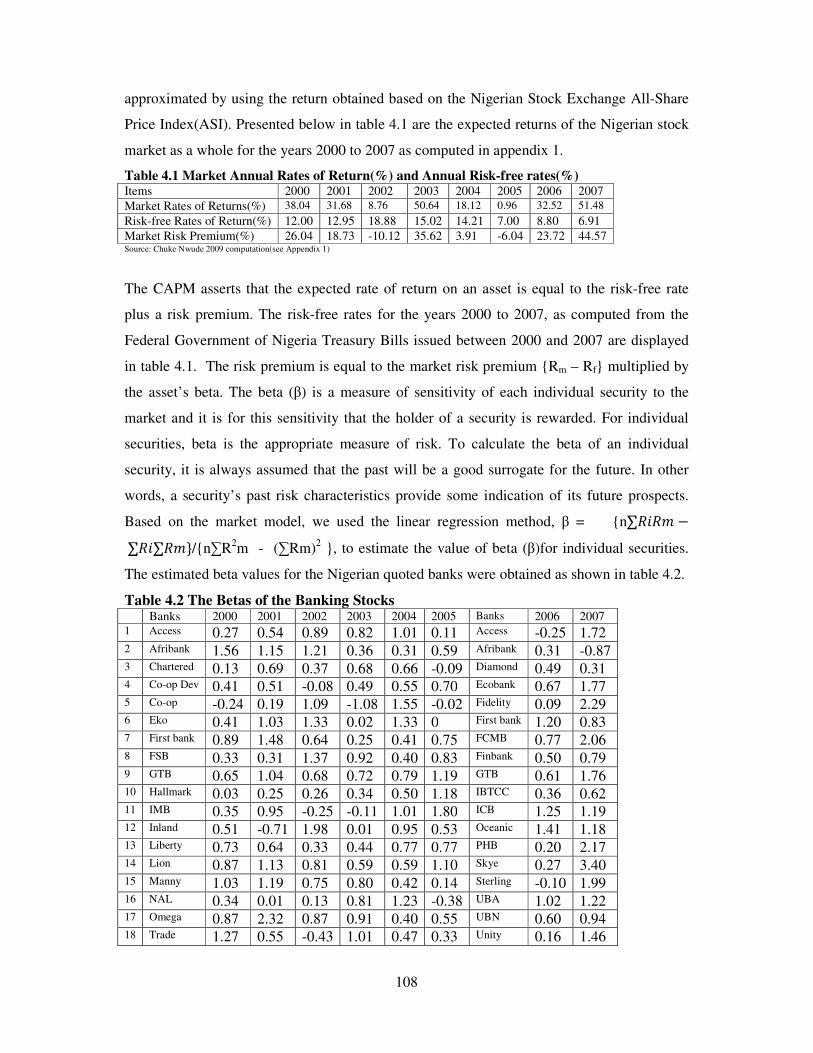
108
approximated by using the return obtained based on the Nigerian Stock Exchange All-Share
Price Index(ASI). Presented below in table 4.1 are the expected returns of the Nigerian stock
market as a whole for the years 2000 to 2007 as computed in appendix 1.
Table 4.1 Market Annual Rates of Return(%) and Annual Risk-free rates(%) Items 2000 2001 2002 2003 2004 2005 2006 2007 Market Rates of Returns(%) 38.04 31.68 8.76 50.64 18.12 0.96 32.52 51.48 Risk-free Rates of Return(%) 12.00 12.95 18.88 15.02 14.21 7.00 8.80 6.91 Market Risk Premium(%) 26.04 18.73 -10.12 35.62 3.91 -6.04 23.72 44.57 Source: Chuke Nwude 2009 computation(see Appendix 1)
The CAPM asserts that the expected rate of return on an asset is equal to the risk-free rate
plus a risk premium. The risk-free rates for the years 2000 to 2007, as computed from the
Federal Government of Nigeria Treasury Bills issued between 2000 and 2007 are displayed
in table 4.1. The risk premium is equal to the market risk premium {Rm – Rf} multiplied by
the asset’s beta. The beta (�) is a measure of sensitivity of each individual security to the
market and it is for this sensitivity that the holder of a security is rewarded. For individual
securities, beta is the appropriate measure of risk. To calculate the beta of an individual
security, it is always assumed that the past will be a good surrogate for the future. In other
words, a security’s past risk characteristics provide some indication of its future prospects.
Based on the market model, we used the linear regression method, � = {n����� �
������� �/{n�R2m - (�Rm)2 }, to estimate the value of beta (�)for individual securities.
The estimated beta values for the Nigerian quoted banks were obtained as shown in table 4.2.
Table 4.2 The Betas of the Banking Stocks Banks 2000 2001 2002 2003 2004 2005 Banks 2006 2007 1 Access 0.27 0.54 0.89 0.82 1.01 0.11 Access -0.25 1.72 2 Afribank 1.56 1.15 1.21 0.36 0.31 0.59 Afribank 0.31 -0.87 3 Chartered 0.13 0.69 0.37 0.68 0.66 -0.09 Diamond 0.49 0.31 4 Co-op Dev 0.41 0.51 -0.08 0.49 0.55 0.70 Ecobank 0.67 1.77 5 Co-op -0.24 0.19 1.09 -1.08 1.55 -0.02 Fidelity 0.09 2.29 6 Eko 0.41 1.03 1.33 0.02 1.33 0 First bank 1.20 0.83 7 First bank 0.89 1.48 0.64 0.25 0.41 0.75 FCMB 0.77 2.06 8 FSB 0.33 0.31 1.37 0.92 0.40 0.83 Finbank 0.50 0.79 9 GTB 0.65 1.04 0.68 0.72 0.79 1.19 GTB 0.61 1.76 10 Hallmark 0.03 0.25 0.26 0.34 0.50 1.18 IBTCC 0.36 0.62 11 IMB 0.35 0.95 -0.25 -0.11 1.01 1.80 ICB 1.25 1.19 12 Inland 0.51 -0.71 1.98 0.01 0.95 0.53 Oceanic 1.41 1.18 13 Liberty 0.73 0.64 0.33 0.44 0.77 0.77 PHB 0.20 2.17 14 Lion 0.87 1.13 0.81 0.59 0.59 1.10 Skye 0.27 3.40 15 Manny 1.03 1.19 0.75 0.80 0.42 0.14 Sterling -0.10 1.99 16 NAL 0.34 0.01 0.13 0.81 1.23 -0.38 UBA 1.02 1.22 17 Omega 0.87 2.32 0.87 0.91 0.40 0.55 UBN 0.60 0.94 18 Trade 1.27 0.55 -0.43 1.01 0.47 0.33 Unity 0.16 1.46
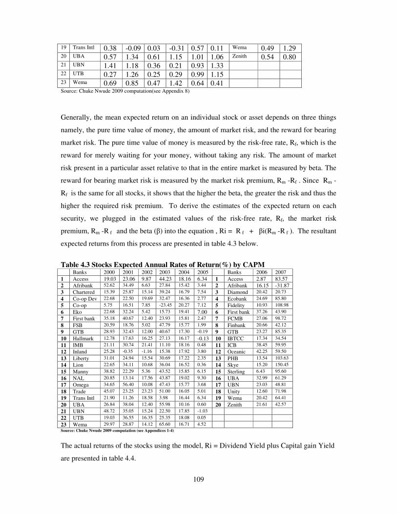
109
19 Trans Intl 0.38 -0.09 0.03 -0.31 0.57 0.11 Wema 0.49 1.29 20 UBA 0.57 1.34 0.61 1.15 1.01 1.06 Zenith 0.54 0.80 21 UBN 1.41 1.18 0.36 0.21 0.93 1.33 22 UTB 0.27 1.26 0.25 0.29 0.99 1.15 23 Wema 0.69 0.85 0.47 1.42 0.64 0.41 Source: Chuke Nwude 2009 computation(see Appendix 8)
Generally, the mean expected return on an individual stock or asset depends on three things
namely, the pure time value of money, the amount of market risk, and the reward for bearing
market risk. The pure time value of money is measured by the risk-free rate, Rf, which is the
reward for merely waiting for your money, without taking any risk. The amount of market
risk present in a particular asset relative to that in the entire market is measured by beta. The
reward for bearing market risk is measured by the market risk premium, Rm -Rf . Since Rm -
Rf is the same for all stocks, it shows that the higher the beta, the greater the risk and thus the
higher the required risk premium. To derive the estimates of the expected return on each
security, we plugged in the estimated values of the risk-free rate, Rf, the market risk
premium, Rm -R f and the beta (�) into the equation , Ri = R f + �i(Rm -R f ). The resultant
expected returns from this process are presented in table 4.3 below.
Table 4.3 Stocks Expected Annual Rates of Return(%) by CAPM Banks 2000 2001 2002 2003 2004 2005 Banks 2006 2007 1 Access 19.03 23.06 9.87 44.23 18.16 6.34 1 Access 2.87 83.57 2 Afribank 52.62 34.49 6.63 27.84 15.42 3.44 2 Afribank 16.15 -31.87 3 Chartered 15.39 25.87 15.14 39.24 16.79 7.54 3 Diamond 20.42 20.73 4 Co-op Dev 22.68 22.50 19.69 32.47 16.36 2.77 4 Ecobank 24.69 85.80 5 Co-op 5.75 16.51 7.85 -23.45 20.27 7.12 5 Fidelity 10.93 108.98 6 Eko 22.68 32.24 5.42 15.73 19.41 7.00 6 First bank 37.26 43.90 7 First bank 35.18 40.67 12.40 23.93 15.81 2.47 7 FCMB 27.06 98.72 8 FSB 20.59 18.76 5.02 47.79 15.77 1.99 8 Finbank 20.66 42.12 9 GTB 28.93 32.43 12.00 40.67 17.30 -0.19 9 GTB 23.27 85.35 10 Hallmark 12.78 17.63 16.25 27.13 16.17 -0.13 10 IBTCC 17.34 34.54 11 IMB 21.11 30.74 21.41 11.10 18.16 0.48 11 ICB 38.45 59.95 12 Inland 25.28 -0.35 -1.16 15.38 17.92 3.80 12 Oceanic 42.25 59.50 13 Liberty 31.01 24.94 15.54 30.69 17.22 2.35 13 PHB 13.54 103.63 14 Lion 22.65 34.11 10.68 36.04 16.52 0.36 14 Skye 15.20 150.45 15 Manny 38.82 22.29 5.36 43.52 15.85 6.15 15 Sterling 6.43 95.60 16 NAL 20.85 13.14 17.56 43.87 19.02 9.30 16 UBA 32.99 61.29 17 Omega 34.65 56.40 10.08 47.43 15.77 3.68 17 UBN 23.03 48.81 18 Trade 45.07 23.25 23.23 51.00 16.05 5.01 18 Unity 12.60 71.98 19 Trans Intl 21.90 11.26 18.58 3.98 16.44 6.34 19 Wema 20.42 64.41 20 UBA 26.84 38.04 12.40 55.98 10.16 0.60 20 Zenith 21.61 42.57 21 UBN 48.72 35.05 15.24 22.50 17.85 -1.03 22 UTB 19.03 36.55 16.35 25.35 18.08 0.05 23 Wema 29.97 28.87 14.12 65.60 16.71 4.52 Source: Chuke Nwude 2009 computation (see Appendices 1-4)
The actual returns of the stocks using the model, Ri = Dividend Yield plus Capital gain Yield
are presented in table 4.4.
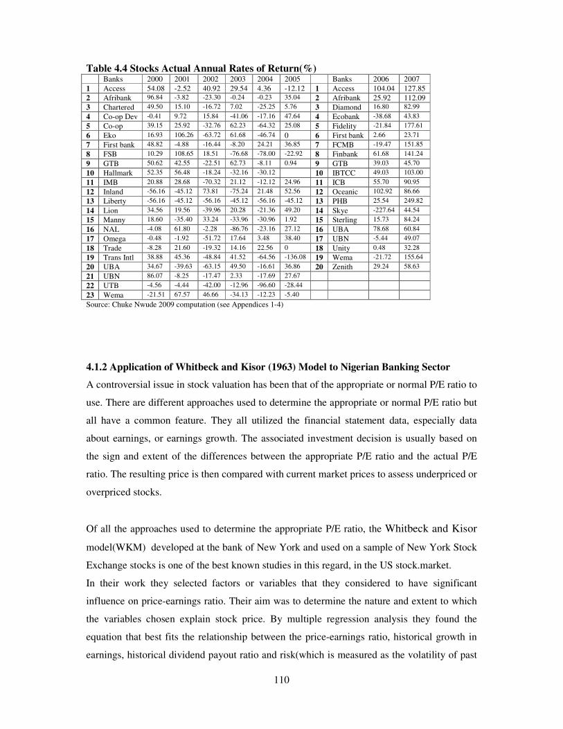
110
Table 4.4 Stocks Actual Annual Rates of Return(%) Banks 2000 2001 2002 2003 2004 2005 Banks 2006 2007 1 Access 54.08 -2.52 40.92 29.54 4.36 -12.12 1 Access 104.04 127.85 2 Afribank 96.84 -3.82 -23.30 -0.24 -0.23 35.04 2 Afribank 25.92 112.09 3 Chartered 49.50 15.10 -16.72 7.02 -25.25 5.76 3 Diamond 16.80 82.99 4 Co-op Dev -0.41 9.72 15.84 -41.06 -17.16 47.64 4 Ecobank -38.68 43.83 5 Co-op 39.15 25.92 -32.76 62.23 -64.32 25.08 5 Fidelity -21.84 177.61 6 Eko 16.93 106.26 -63.72 61.68 -46.74 0 6 First bank 2.66 23.71 7 First bank 48.82 -4.88 -16.44 -8.20 24.21 36.85 7 FCMB -19.47 151.85 8 FSB 10.29 108.65 18.51 -76.68 -78.00 -22.92 8 Finbank 61.68 141.24 9 GTB 50.62 42.55 -22.51 62.73 -8.11 0.94 9 GTB 39.03 45.70 10 Hallmark 52.35 56.48 -18.24 -32.16 -30.12 10 IBTCC 49.03 103.00 11 IMB 20.88 28.68 -70.32 21.12 -12.12 24.96 11 ICB 55.70 90.95 12 Inland -56.16 -45.12 73.81 -75.24 21.48 52.56 12 Oceanic 102.92 86.66 13 Liberty -56.16 -45.12 -56.16 -45.12 -56.16 -45.12 13 PHB 25.54 249.82 14 Lion 34.56 19.56 -39.96 20.28 -21.36 49.20 14 Skye -227.64 44.54 15 Manny 18.60 -35.40 33.24 -33.96 -30.96 1.92 15 Sterling 15.73 84.24 16 NAL -4.08 61.80 -2.28 -86.76 -23.16 27.12 16 UBA 78.68 60.84 17 Omega -0.48 -1.92 -51.72 17.64 3.48 38.40 17 UBN -5.44 49.07 18 Trade -8.28 21.60 -19.32 14.16 22.56 0 18 Unity 0.48 32.28 19 Trans Intl 38.88 45.36 -48.84 41.52 -64.56 -136.08 19 Wema -21.72 155.64 20 UBA 34.67 -39.63 -63.15 49.50 -16.61 36.86 20 Zenith 29.24 58.63 21 UBN 86.07 -8.25 -17.47 2.33 -17.69 27.67 22 UTB -4.56 -4.44 -42.00 -12.96 -96.60 -28.44 23 Wema -21.51 67.57 46.66 -34.13 -12.23 -5.40 Source: Chuke Nwude 2009 computation (see Appendices 1-4) 4.1.2 Application of Whitbeck and Kisor (1963) Model to Nigerian Banking Sector
A controversial issue in stock valuation has been that of the appropriate or normal P/E ratio to
use. There are different approaches used to determine the appropriate or normal P/E ratio but
all have a common feature. They all utilized the financial statement data, especially data
about earnings, or earnings growth. The associated investment decision is usually based on
the sign and extent of the differences between the appropriate P/E ratio and the actual P/E
ratio. The resulting price is then compared with current market prices to assess underpriced or
overpriced stocks.
Of all the approaches used to determine the appropriate P/E ratio, the Whitbeck and Kisor
model(WKM) developed at the bank of New York and used on a sample of New York Stock
Exchange stocks is one of the best known studies in this regard, in the US stock.market.
In their work they selected factors or variables that they considered to have significant
influence on price-earnings ratio. Their aim was to determine the nature and extent to which
the variables chosen explain stock price. By multiple regression analysis they found the
equation that best fits the relationship between the price-earnings ratio, historical growth in
earnings, historical dividend payout ratio and risk(which is measured as the volatility of past
111
earnings around the trend). The assumption here was that the differences in P/E’s between
stocks can be explained by projected earnings growth, expected dividend payout, and the
variability in the rate of earnings growth or growth risk. The WKM estimated the relationship
existing among these variables by the equation,
Pi/Ei = �i + �1Gi + �2PRi + �3Ri
Where
� = the constant term of the regression equation. It gives the value of P/E
ratio when all the independent variables assume zero value.
� = the slopes of the regression equation. It measures the value the P/E
ratio will assume if each of the variables changes by a unit.
Gi = the expected rate of growth in earnings per share of each bank.
PR = the expected dividend payout ratio of each bank
R = the expected standard deviation of earnings around the mean
The equation gives an estimate of the simultaneous impact of the three factors on the level of
the price-earnings ratio. The signs tell us the expected direction of the impact. The equation
could be used for share selection by computing the values of the three variables for any share
and determine the appropriate P/E ratio. Then the appropriate P/E ratio is compared with the
current P/E ratio. The decision rule is that a share should be sold if the appropriate P/E ratio
is below the current P/E ratio, and be bought if the appropriate P/E ratio is above the current
P/E ratio. The result of Whitbeck and Kisor (1963) study gave the predictive equation
as:
Price-earnings ratio = 8.2 + (1.5 x earnings growth) + (6.7 x Payout ratio) - (0.2 x
standard deviation of earnings)
With this result, they concluded that P/E ratio is an increasing function of earnings growth
and dividend payout and inversely related to the variation in the earnings growth rate. In
other words, higher P/Es were associated with higher growth and payout and less variation in
the growth rate. That is, the P/E ratio fell as risk increased.
In this study, the model has been tested on a representative sample of 20 pre-consolidation
banks stocks and 20 post-consolidation banks stocks quoted on the Nigerian Stock Exchange
to estimate the relationship between the price-earnings ratio, historical growth in earnings,
historical dividend payout ratio and risk(which is measured as the volatility of past earnings
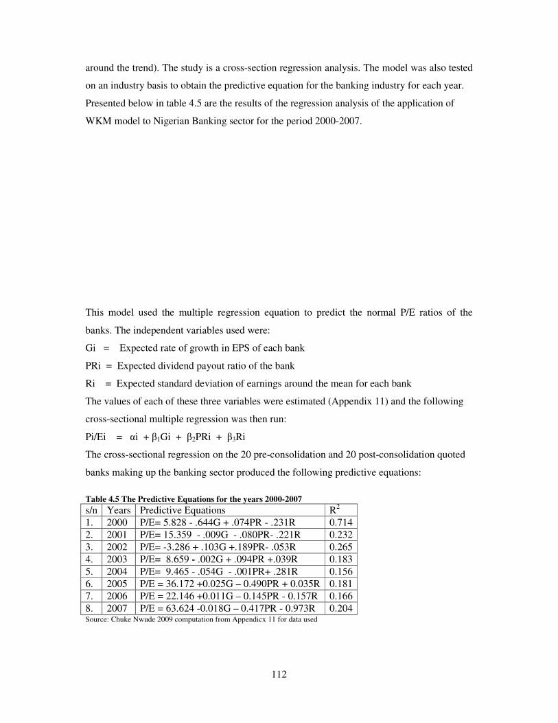
112
around the trend). The study is a cross-section regression analysis. The model was also tested
on an industry basis to obtain the predictive equation for the banking industry for each year.
Presented below in table 4.5 are the results of the regression analysis of the application of
WKM model to Nigerian Banking sector for the period 2000-2007.
This model used the multiple regression equation to predict the normal P/E ratios of the
banks. The independent variables used were:
Gi = Expected rate of growth in EPS of each bank
PRi = Expected dividend payout ratio of the bank
Ri = Expected standard deviation of earnings around the mean for each bank
The values of each of these three variables were estimated (Appendix 11) and the following
cross-sectional multiple regression was then run:
Pi/Ei = �i + �1Gi + �2PRi + �3Ri
The cross-sectional regression on the 20 pre-consolidation and 20 post-consolidation quoted
banks making up the banking sector produced the following predictive equations:
Table 4.5 The Predictive Equations for the years 2000-2007 s/n Years Predictive Equations R2 1. 2000 P/E= 5.828 - .644G + .074PR - .231R 0.714 2. 2001 P/E= 15.359 - .009G - .080PR- .221R 0.232 3. 2002 P/E= -3.286 + .103G +.189PR- .053R 0.265 4. 2003 P/E= 8.659 - .002G + .094PR +.039R 0.183 5. 2004 P/E= 9.465 - .054G - .001PR+ .281R 0.156 6. 2005 P/E = 36.172 +0.025G – 0.490PR + 0.035R 0.181 7. 2006 P/E = 22.146 +0.011G – 0.145PR - 0.157R 0.166 8. 2007 P/E = 63.624 -0.018G – 0.417PR - 0.973R 0.204 Source: Chuke Nwude 2009 computation from Appendicx 11 for data used
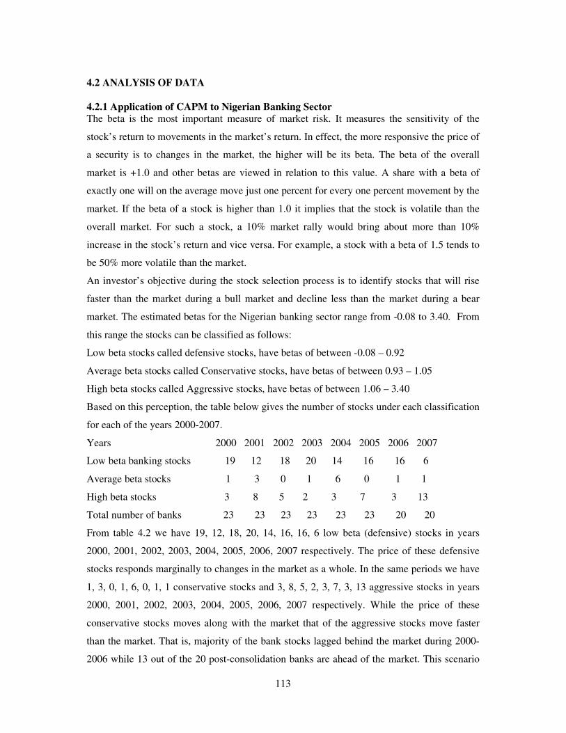
113
4.2 ANALYSIS OF DATA 4.2.1 Application of CAPM to Nigerian Banking Sector The beta is the most important measure of market risk. It measures the sensitivity of the
stock’s return to movements in the market’s return. In effect, the more responsive the price of
a security is to changes in the market, the higher will be its beta. The beta of the overall
market is +1.0 and other betas are viewed in relation to this value. A share with a beta of
exactly one will on the average move just one percent for every one percent movement by the
market. If the beta of a stock is higher than 1.0 it implies that the stock is volatile than the
overall market. For such a stock, a 10% market rally would bring about more than 10%
increase in the stock’s return and vice versa. For example, a stock with a beta of 1.5 tends to
be 50% more volatile than the market.
An investor’s objective during the stock selection process is to identify stocks that will rise
faster than the market during a bull market and decline less than the market during a bear
market. The estimated betas for the Nigerian banking sector range from -0.08 to 3.40. From
this range the stocks can be classified as follows:
Low beta stocks called defensive stocks, have betas of between -0.08 – 0.92
Average beta stocks called Conservative stocks, have betas of between 0.93 – 1.05
High beta stocks called Aggressive stocks, have betas of between 1.06 – 3.40
Based on this perception, the table below gives the number of stocks under each classification
for each of the years 2000-2007.
Years 2000 2001 2002 2003 2004 2005 2006 2007
Low beta banking stocks 19 12 18 20 14 16 16 6
Average beta stocks 1 3 0 1 6 0 1 1
High beta stocks 3 8 5 2 3 7 3 13
Total number of banks 23 23 23 23 23 23 20 20
From table 4.2 we have 19, 12, 18, 20, 14, 16, 16, 6 low beta (defensive) stocks in years
2000, 2001, 2002, 2003, 2004, 2005, 2006, 2007 respectively. The price of these defensive
stocks responds marginally to changes in the market as a whole. In the same periods we have
1, 3, 0, 1, 6, 0, 1, 1 conservative stocks and 3, 8, 5, 2, 3, 7, 3, 13 aggressive stocks in years
2000, 2001, 2002, 2003, 2004, 2005, 2006, 2007 respectively. While the price of these
conservative stocks moves along with the market that of the aggressive stocks move faster
than the market. That is, majority of the bank stocks lagged behind the market during 2000-
2006 while 13 out of the 20 post-consolidation banks are ahead of the market. This scenario
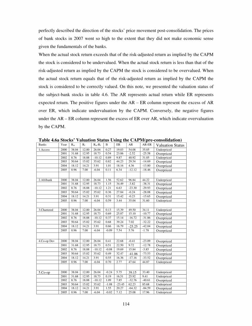
114
perfectly described the direction of the stocks’ price movement post-consolidation. The prices
of bank stocks in 2007 went so high to the extent that they did not make economic sense
given the fundamentals of the banks.
When the actual stock return exceeds that of the risk-adjusted return as implied by the CAPM
the stock is considered to be undervalued. When the actual stock return is less than that of the
risk-adjusted return as implied by the CAPM the stock is considered to be overvalued. When
the actual stock return equals that of the risk-adjusted return as implied by the CAPM the
stock is considered to be correctly valued. On this note, we presented the valuation status of
the subject-bank stocks in table 4.6. The AR represents actual return while ER represents
expected return. The positive figures under the AR – ER column represent the excess of AR
over ER, which indicate undervaluation by the CAPM. Conversely, the negative figures
under the AR – ER column represent the excess of ER over AR, which indicate overvaluation
by the CAPM.
Table 4.6a Stocks’ Valuation Status Using the CAPM(pre-consolidation) Banks Year Rm Rf Rm-Rf � ER AR AR-ER Valuation Status 1.Access 2000 38.04 12.00 26.04 0.27 19.03 54.08 35.05 Underpriced 2001 31.68 12.95 18.73 0.54 23.06 -2.52 -25.58 Overpriced 2002 8.76 18.88 -10.12 0.89 9.87 40.92 31.05 Underpriced 2003 50.64 15.02 35.62 0.82 44.23 29.54 -14.69 Overpriced 2004 18.12 14.21 3.91 1.01 18.16 4.36 -13.80 Overpriced 2005 0.96 7.00 -6.04 0.11 6.34 -12.12 -18.46 Overpriced 2.Afribank 2000 38.04 12.00 26.04 1.56 52.62 96.84 44.22 Underpriced 2001 31.68 12.95 18.73 1.15 34.49 -3.82 -38.31 Overpriced 2002 8.76 18.88 -10.12 1.21 6.63 -23.30 -29.93 Overpriced 2003 50.64 15.02 35.62 0.36 27.84 -0.24 -28.08 Overpriced 2004 18.12 14.21 3.91 0.31 15.42 -0.23 -15.65 Overpriced 2005 0.96 7.00 -6.04 0.59 3.44 35.04 31.60 Underpriced 3.Chartered 2000 38.04 12.00 26.04 0.13 15.39 49.50 34.11 Underpriced 2001 31.68 12.95 18.73 0.69 25.87 15.10 -10.77 Overpriced 2002 8.76 18.88 -10.12 0.37 15.14 -16.72 -31.86 Overpriced 2003 50.64 15.02 35.62 0.68 39.24 7.02 -32.22 Overpriced 2004 18.12 14.21 3.91 0.66 16.79 -25.25 -42.04 Overpriced 2005 0.96 7.00 -6.04 -0.09 7.54 5.76 -1.78 Overpriced 4.Co-op Dev 2000 38.04 12.00 26.04 0.41 22.68 -0.41 -23.09 Overpriced 2001 31.68 12.95 18.73 0.51 22.50 9.72 -12.78 Overpriced 2002 8.76 18.88 -10.12 -0.08 19.69 15.84 -3.85 Overpriced 2003 50.64 15.02 35.62 0.49 32.47 -41.06 -73.53 Overpriced 2004 18.12 14.21 3.91 0.55 16.36 -17.16 -33.52 Overpriced 2005 0.96 7.00 -6.04 0.70 2.77 47.64 44.87 Underpriced 5.Co-op 2000 38.04 12.00 26.04 -0.24 5.75 39.15 33.40 Underpriced 2001 31.68 12.95 18.73 0.19 16.51 25.92 9.41 Underpriced 2002 8.76 18.88 -10.12 1.09 7.85 -32.76 -40.61 Overpriced 2003 50.64 15.02 35.62 -1.08 -23.45 62.23 85.68 Underpriced 2004 18.12 14.21 3.91 1.55 20.27 -64.32 -84.59 Overpriced 2005 0.96 7.00 -6.04 -0.02 7.12 25.08 17.96 Underpriced
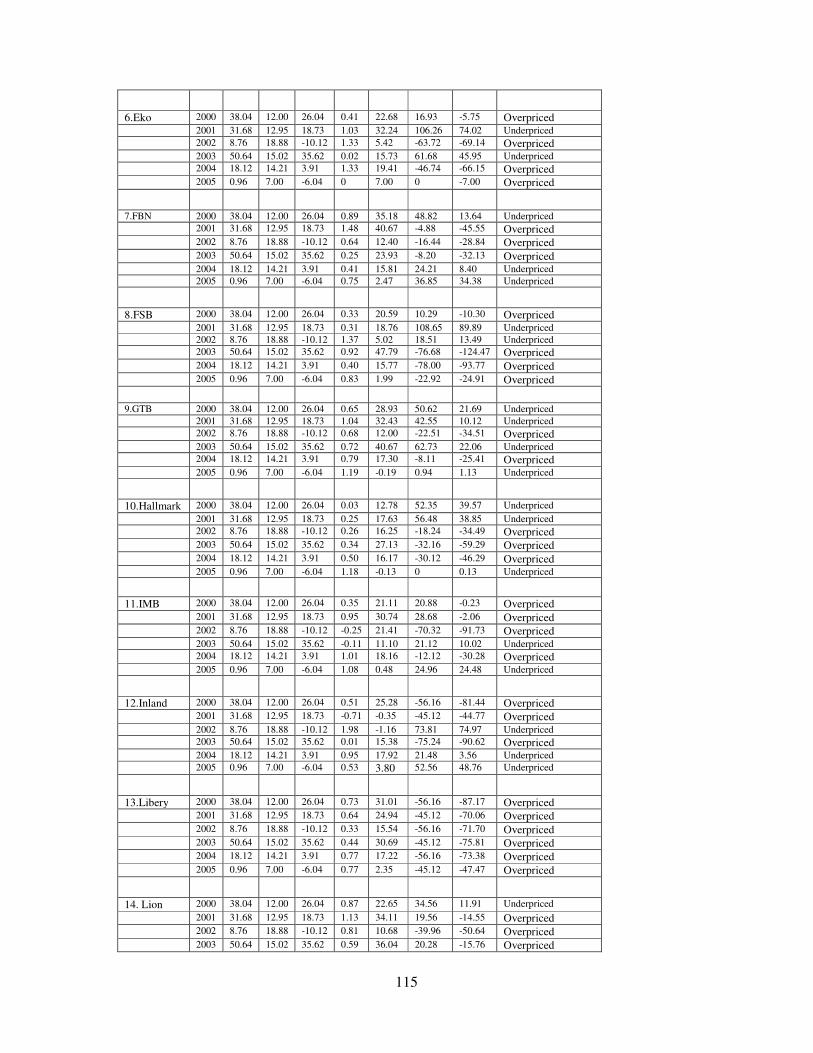
115
6.Eko 2000 38.04 12.00 26.04 0.41 22.68 16.93 -5.75 Overpriced 2001 31.68 12.95 18.73 1.03 32.24 106.26 74.02 Underpriced 2002 8.76 18.88 -10.12 1.33 5.42 -63.72 -69.14 Overpriced 2003 50.64 15.02 35.62 0.02 15.73 61.68 45.95 Underpriced 2004 18.12 14.21 3.91 1.33 19.41 -46.74 -66.15 Overpriced 2005 0.96 7.00 -6.04 0 7.00 0 -7.00 Overpriced 7.FBN 2000 38.04 12.00 26.04 0.89 35.18 48.82 13.64 Underpriced 2001 31.68 12.95 18.73 1.48 40.67 -4.88 -45.55 Overpriced 2002 8.76 18.88 -10.12 0.64 12.40 -16.44 -28.84 Overpriced 2003 50.64 15.02 35.62 0.25 23.93 -8.20 -32.13 Overpriced 2004 18.12 14.21 3.91 0.41 15.81 24.21 8.40 Underpriced 2005 0.96 7.00 -6.04 0.75 2.47 36.85 34.38 Underpriced 8.FSB 2000 38.04 12.00 26.04 0.33 20.59 10.29 -10.30 Overpriced 2001 31.68 12.95 18.73 0.31 18.76 108.65 89.89 Underpriced 2002 8.76 18.88 -10.12 1.37 5.02 18.51 13.49 Underpriced 2003 50.64 15.02 35.62 0.92 47.79 -76.68 -124.47 Overpriced 2004 18.12 14.21 3.91 0.40 15.77 -78.00 -93.77 Overpriced 2005 0.96 7.00 -6.04 0.83 1.99 -22.92 -24.91 Overpriced 9.GTB 2000 38.04 12.00 26.04 0.65 28.93 50.62 21.69 Underpriced 2001 31.68 12.95 18.73 1.04 32.43 42.55 10.12 Underpriced 2002 8.76 18.88 -10.12 0.68 12.00 -22.51 -34.51 Overpriced 2003 50.64 15.02 35.62 0.72 40.67 62.73 22.06 Underpriced 2004 18.12 14.21 3.91 0.79 17.30 -8.11 -25.41 Overpriced 2005 0.96 7.00 -6.04 1.19 -0.19 0.94 1.13 Underpriced 10.Hallmark 2000 38.04 12.00 26.04 0.03 12.78 52.35 39.57 Underpriced 2001 31.68 12.95 18.73 0.25 17.63 56.48 38.85 Underpriced 2002 8.76 18.88 -10.12 0.26 16.25 -18.24 -34.49 Overpriced 2003 50.64 15.02 35.62 0.34 27.13 -32.16 -59.29 Overpriced 2004 18.12 14.21 3.91 0.50 16.17 -30.12 -46.29 Overpriced 2005 0.96 7.00 -6.04 1.18 -0.13 0 0.13 Underpriced 11.IMB 2000 38.04 12.00 26.04 0.35 21.11 20.88 -0.23 Overpriced 2001 31.68 12.95 18.73 0.95 30.74 28.68 -2.06 Overpriced 2002 8.76 18.88 -10.12 -0.25 21.41 -70.32 -91.73 Overpriced 2003 50.64 15.02 35.62 -0.11 11.10 21.12 10.02 Underpriced 2004 18.12 14.21 3.91 1.01 18.16 -12.12 -30.28 Overpriced 2005 0.96 7.00 -6.04 1.08 0.48 24.96 24.48 Underpriced 12.Inland 2000 38.04 12.00 26.04 0.51 25.28 -56.16 -81.44 Overpriced 2001 31.68 12.95 18.73 -0.71 -0.35 -45.12 -44.77 Overpriced 2002 8.76 18.88 -10.12 1.98 -1.16 73.81 74.97 Underpriced 2003 50.64 15.02 35.62 0.01 15.38 -75.24 -90.62 Overpriced 2004 18.12 14.21 3.91 0.95 17.92 21.48 3.56 Underpriced 2005 0.96 7.00 -6.04 0.53 3.80 52.56 48.76 Underpriced 13.Libery 2000 38.04 12.00 26.04 0.73 31.01 -56.16 -87.17 Overpriced 2001 31.68 12.95 18.73 0.64 24.94 -45.12 -70.06 Overpriced 2002 8.76 18.88 -10.12 0.33 15.54 -56.16 -71.70 Overpriced 2003 50.64 15.02 35.62 0.44 30.69 -45.12 -75.81 Overpriced 2004 18.12 14.21 3.91 0.77 17.22 -56.16 -73.38 Overpriced 2005 0.96 7.00 -6.04 0.77 2.35 -45.12 -47.47 Overpriced 14. Lion 2000 38.04 12.00 26.04 0.87 22.65 34.56 11.91 Underpriced 2001 31.68 12.95 18.73 1.13 34.11 19.56 -14.55 Overpriced 2002 8.76 18.88 -10.12 0.81 10.68 -39.96 -50.64 Overpriced 2003 50.64 15.02 35.62 0.59 36.04 20.28 -15.76 Overpriced
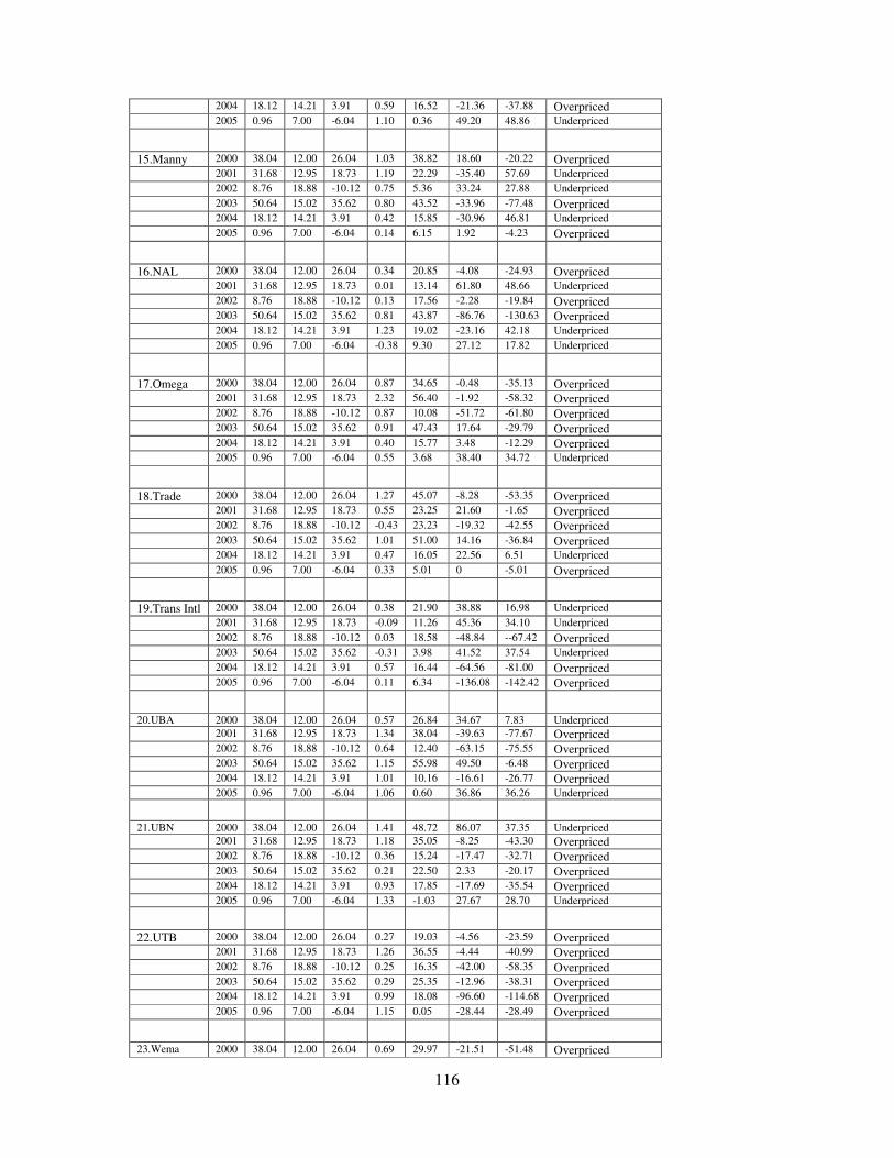
116
2004 18.12 14.21 3.91 0.59 16.52 -21.36 -37.88 Overpriced 2005 0.96 7.00 -6.04 1.10 0.36 49.20 48.86 Underpriced 15.Manny 2000 38.04 12.00 26.04 1.03 38.82 18.60 -20.22 Overpriced 2001 31.68 12.95 18.73 1.19 22.29 -35.40 57.69 Underpriced 2002 8.76 18.88 -10.12 0.75 5.36 33.24 27.88 Underpriced 2003 50.64 15.02 35.62 0.80 43.52 -33.96 -77.48 Overpriced 2004 18.12 14.21 3.91 0.42 15.85 -30.96 46.81 Underpriced 2005 0.96 7.00 -6.04 0.14 6.15 1.92 -4.23 Overpriced 16.NAL 2000 38.04 12.00 26.04 0.34 20.85 -4.08 -24.93 Overpriced 2001 31.68 12.95 18.73 0.01 13.14 61.80 48.66 Underpriced 2002 8.76 18.88 -10.12 0.13 17.56 -2.28 -19.84 Overpriced 2003 50.64 15.02 35.62 0.81 43.87 -86.76 -130.63 Overpriced 2004 18.12 14.21 3.91 1.23 19.02 -23.16 42.18 Underpriced 2005 0.96 7.00 -6.04 -0.38 9.30 27.12 17.82 Underpriced 17.Omega 2000 38.04 12.00 26.04 0.87 34.65 -0.48 -35.13 Overpriced 2001 31.68 12.95 18.73 2.32 56.40 -1.92 -58.32 Overpriced 2002 8.76 18.88 -10.12 0.87 10.08 -51.72 -61.80 Overpriced 2003 50.64 15.02 35.62 0.91 47.43 17.64 -29.79 Overpriced 2004 18.12 14.21 3.91 0.40 15.77 3.48 -12.29 Overpriced 2005 0.96 7.00 -6.04 0.55 3.68 38.40 34.72 Underpriced 18.Trade 2000 38.04 12.00 26.04 1.27 45.07 -8.28 -53.35 Overpriced 2001 31.68 12.95 18.73 0.55 23.25 21.60 -1.65 Overpriced 2002 8.76 18.88 -10.12 -0.43 23.23 -19.32 -42.55 Overpriced 2003 50.64 15.02 35.62 1.01 51.00 14.16 -36.84 Overpriced 2004 18.12 14.21 3.91 0.47 16.05 22.56 6.51 Underpriced 2005 0.96 7.00 -6.04 0.33 5.01 0 -5.01 Overpriced 19.Trans Intl 2000 38.04 12.00 26.04 0.38 21.90 38.88 16.98 Underpriced 2001 31.68 12.95 18.73 -0.09 11.26 45.36 34.10 Underpriced 2002 8.76 18.88 -10.12 0.03 18.58 -48.84 --67.42 Overpriced 2003 50.64 15.02 35.62 -0.31 3.98 41.52 37.54 Underpriced 2004 18.12 14.21 3.91 0.57 16.44 -64.56 -81.00 Overpriced 2005 0.96 7.00 -6.04 0.11 6.34 -136.08 -142.42 Overpriced 20.UBA 2000 38.04 12.00 26.04 0.57 26.84 34.67 7.83 Underpriced 2001 31.68 12.95 18.73 1.34 38.04 -39.63 -77.67 Overpriced 2002 8.76 18.88 -10.12 0.64 12.40 -63.15 -75.55 Overpriced 2003 50.64 15.02 35.62 1.15 55.98 49.50 -6.48 Overpriced 2004 18.12 14.21 3.91 1.01 10.16 -16.61 -26.77 Overpriced 2005 0.96 7.00 -6.04 1.06 0.60 36.86 36.26 Underpriced 21.UBN 2000 38.04 12.00 26.04 1.41 48.72 86.07 37.35 Underpriced 2001 31.68 12.95 18.73 1.18 35.05 -8.25 -43.30 Overpriced 2002 8.76 18.88 -10.12 0.36 15.24 -17.47 -32.71 Overpriced 2003 50.64 15.02 35.62 0.21 22.50 2.33 -20.17 Overpriced 2004 18.12 14.21 3.91 0.93 17.85 -17.69 -35.54 Overpriced 2005 0.96 7.00 -6.04 1.33 -1.03 27.67 28.70 Underpriced 22.UTB 2000 38.04 12.00 26.04 0.27 19.03 -4.56 -23.59 Overpriced 2001 31.68 12.95 18.73 1.26 36.55 -4.44 -40.99 Overpriced 2002 8.76 18.88 -10.12 0.25 16.35 -42.00 -58.35 Overpriced 2003 50.64 15.02 35.62 0.29 25.35 -12.96 -38.31 Overpriced 2004 18.12 14.21 3.91 0.99 18.08 -96.60 -114.68 Overpriced 2005 0.96 7.00 -6.04 1.15 0.05 -28.44 -28.49 Overpriced 23.Wema 2000 38.04 12.00 26.04 0.69 29.97 -21.51 -51.48 Overpriced
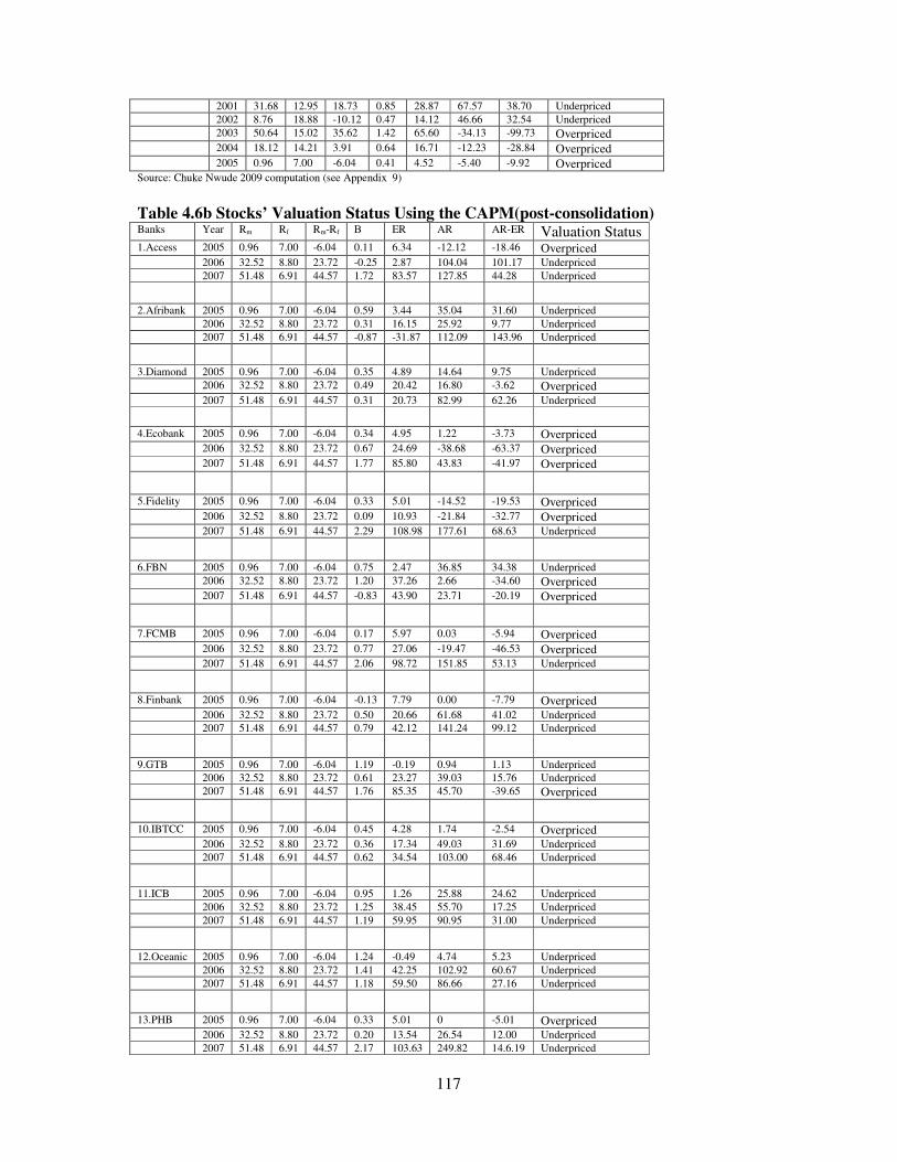
117
2001 31.68 12.95 18.73 0.85 28.87 67.57 38.70 Underpriced 2002 8.76 18.88 -10.12 0.47 14.12 46.66 32.54 Underpriced 2003 50.64 15.02 35.62 1.42 65.60 -34.13 -99.73 Overpriced 2004 18.12 14.21 3.91 0.64 16.71 -12.23 -28.84 Overpriced 2005 0.96 7.00 -6.04 0.41 4.52 -5.40 -9.92 Overpriced Source: Chuke Nwude 2009 computation (see Appendix 9)
Table 4.6b Stocks’ Valuation Status Using the CAPM(post-consolidation) Banks Year Rm Rf Rm-Rf � ER AR AR-ER Valuation Status 1.Access 2005 0.96 7.00 -6.04 0.11 6.34 -12.12 -18.46 Overpriced 2006 32.52 8.80 23.72 -0.25 2.87 104.04 101.17 Underpriced 2007 51.48 6.91 44.57 1.72 83.57 127.85 44.28 Underpriced 2.Afribank 2005 0.96 7.00 -6.04 0.59 3.44 35.04 31.60 Underpriced 2006 32.52 8.80 23.72 0.31 16.15 25.92 9.77 Underpriced 2007 51.48 6.91 44.57 -0.87 -31.87 112.09 143.96 Underpriced 3.Diamond 2005 0.96 7.00 -6.04 0.35 4.89 14.64 9.75 Underpriced 2006 32.52 8.80 23.72 0.49 20.42 16.80 -3.62 Overpriced 2007 51.48 6.91 44.57 0.31 20.73 82.99 62.26 Underpriced 4.Ecobank 2005 0.96 7.00 -6.04 0.34 4.95 1.22 -3.73 Overpriced 2006 32.52 8.80 23.72 0.67 24.69 -38.68 -63.37 Overpriced 2007 51.48 6.91 44.57 1.77 85.80 43.83 -41.97 Overpriced 5.Fidelity 2005 0.96 7.00 -6.04 0.33 5.01 -14.52 -19.53 Overpriced 2006 32.52 8.80 23.72 0.09 10.93 -21.84 -32.77 Overpriced 2007 51.48 6.91 44.57 2.29 108.98 177.61 68.63 Underpriced 6.FBN 2005 0.96 7.00 -6.04 0.75 2.47 36.85 34.38 Underpriced 2006 32.52 8.80 23.72 1.20 37.26 2.66 -34.60 Overpriced 2007 51.48 6.91 44.57 -0.83 43.90 23.71 -20.19 Overpriced 7.FCMB 2005 0.96 7.00 -6.04 0.17 5.97 0.03 -5.94 Overpriced 2006 32.52 8.80 23.72 0.77 27.06 -19.47 -46.53 Overpriced 2007 51.48 6.91 44.57 2.06 98.72 151.85 53.13 Underpriced 8.Finbank 2005 0.96 7.00 -6.04 -0.13 7.79 0.00 -7.79 Overpriced 2006 32.52 8.80 23.72 0.50 20.66 61.68 41.02 Underpriced 2007 51.48 6.91 44.57 0.79 42.12 141.24 99.12 Underpriced 9.GTB 2005 0.96 7.00 -6.04 1.19 -0.19 0.94 1.13 Underpriced 2006 32.52 8.80 23.72 0.61 23.27 39.03 15.76 Underpriced 2007 51.48 6.91 44.57 1.76 85.35 45.70 -39.65 Overpriced 10.IBTCC 2005 0.96 7.00 -6.04 0.45 4.28 1.74 -2.54 Overpriced 2006 32.52 8.80 23.72 0.36 17.34 49.03 31.69 Underpriced 2007 51.48 6.91 44.57 0.62 34.54 103.00 68.46 Underpriced 11.ICB 2005 0.96 7.00 -6.04 0.95 1.26 25.88 24.62 Underpriced 2006 32.52 8.80 23.72 1.25 38.45 55.70 17.25 Underpriced 2007 51.48 6.91 44.57 1.19 59.95 90.95 31.00 Underpriced 12.Oceanic 2005 0.96 7.00 -6.04 1.24 -0.49 4.74 5.23 Underpriced 2006 32.52 8.80 23.72 1.41 42.25 102.92 60.67 Underpriced 2007 51.48 6.91 44.57 1.18 59.50 86.66 27.16 Underpriced 13.PHB 2005 0.96 7.00 -6.04 0.33 5.01 0 -5.01 Overpriced 2006 32.52 8.80 23.72 0.20 13.54 26.54 12.00 Underpriced 2007 51.48 6.91 44.57 2.17 103.63 249.82 14.6.19 Underpriced
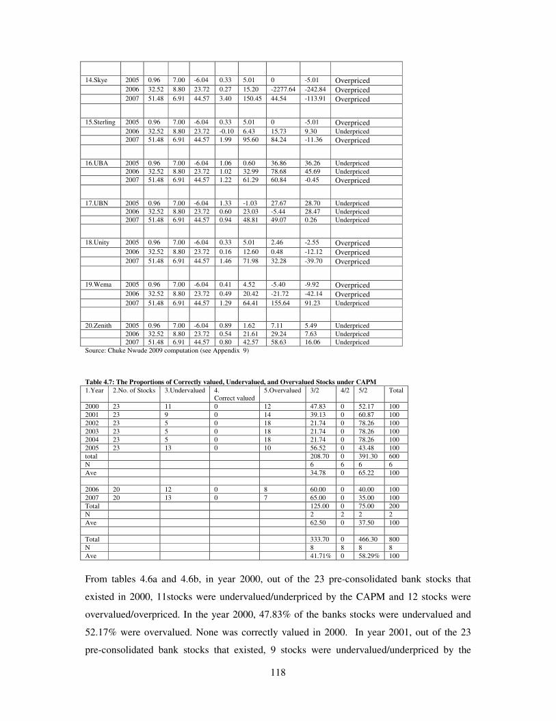
118
14.Skye 2005 0.96 7.00 -6.04 0.33 5.01 0 -5.01 Overpriced 2006 32.52 8.80 23.72 0.27 15.20 -2277.64 -242.84 Overpriced 2007 51.48 6.91 44.57 3.40 150.45 44.54 -113.91 Overpriced 15.Sterling 2005 0.96 7.00 -6.04 0.33 5.01 0 -5.01 Overpriced 2006 32.52 8.80 23.72 -0.10 6.43 15.73 9.30 Underpriced 2007 51.48 6.91 44.57 1.99 95.60 84.24 -11.36 Overpriced 16.UBA 2005 0.96 7.00 -6.04 1.06 0.60 36.86 36.26 Underpriced 2006 32.52 8.80 23.72 1.02 32.99 78.68 45.69 Underpriced 2007 51.48 6.91 44.57 1.22 61.29 60.84 -0.45 Overpriced 17.UBN 2005 0.96 7.00 -6.04 1.33 -1.03 27.67 28.70 Underpriced 2006 32.52 8.80 23.72 0.60 23.03 -5.44 28.47 Underpriced 2007 51.48 6.91 44.57 0.94 48.81 49.07 0.26 Underpriced 18.Unity 2005 0.96 7.00 -6.04 0.33 5.01 2.46 -2.55 Overpriced 2006 32.52 8.80 23.72 0.16 12.60 0.48 -12.12 Overpriced 2007 51.48 6.91 44.57 1.46 71.98 32.28 -39.70 Overpriced 19.Wema 2005 0.96 7.00 -6.04 0.41 4.52 -5.40 -9.92 Overpriced 2006 32.52 8.80 23.72 0.49 20.42 -21.72 -42.14 Overpriced 2007 51.48 6.91 44.57 1.29 64.41 155.64 91.23 Underpriced 20.Zenith 2005 0.96 7.00 -6.04 0.89 1.62 7.11 5.49 Underpriced 2006 32.52 8.80 23.72 0.54 21.61 29.24 7.63 Underpriced 2007 51.48 6.91 44.57 0.80 42.57 58.63 16.06 Underpriced Source: Chuke Nwude 2009 computation (see Appendix 9) Table 4.7: The Proportions of Correctly valued, Undervalued, and Overvalued Stocks under CAPM 1.Year 2.No. of Stocks 3.Undervalued 4.
Correct valued 5.Overvalued 3/2 4/2 5/2 Total
2000 23 11 0 12 47.83 0 52.17 100 2001 23 9 0 14 39.13 0 60.87 100 2002 23 5 0 18 21.74 0 78.26 100 2003 23 5 0 18 21.74 0 78.26 100 2004 23 5 0 18 21.74 0 78.26 100 2005 23 13 0 10 56.52 0 43.48 100 total 208.70 0 391.30 600 N 6 6 6 6 Ave 34.78 0 65.22 100 2006 20 12 0 8 60.00 0 40.00 100 2007 20 13 0 7 65.00 0 35.00 100 Total 125.00 0 75.00 200 N 2 2 2 2 Ave 62.50 0 37.50 100 Total 333.70 0 466.30 800 N 8 8 8 8 Ave 41.71% 0 58.29% 100
From tables 4.6a and 4.6b, in year 2000, out of the 23 pre-consolidated bank stocks that
existed in 2000, 11stocks were undervalued/underpriced by the CAPM and 12 stocks were
overvalued/overpriced. In the year 2000, 47.83% of the banks stocks were undervalued and
52.17% were overvalued. None was correctly valued in 2000. In year 2001, out of the 23
pre-consolidated bank stocks that existed, 9 stocks were undervalued/underpriced by the
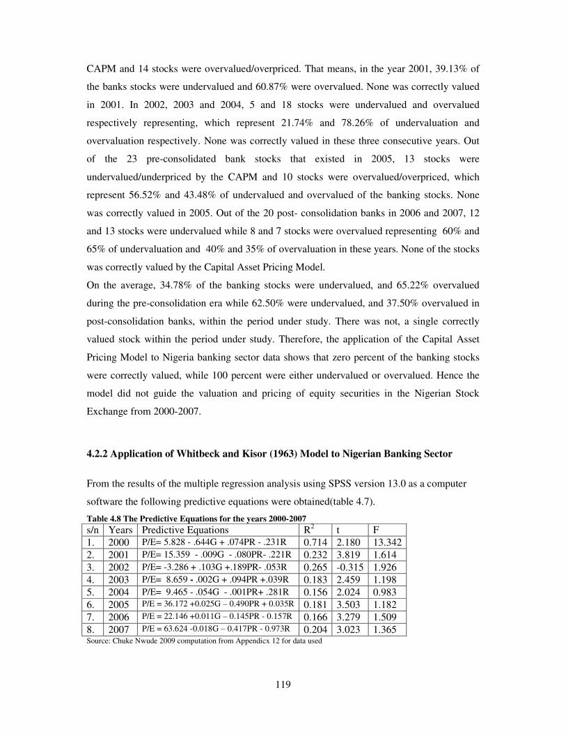
119
CAPM and 14 stocks were overvalued/overpriced. That means, in the year 2001, 39.13% of
the banks stocks were undervalued and 60.87% were overvalued. None was correctly valued
in 2001. In 2002, 2003 and 2004, 5 and 18 stocks were undervalued and overvalued
respectively representing, which represent 21.74% and 78.26% of undervaluation and
overvaluation respectively. None was correctly valued in these three consecutive years. Out
of the 23 pre-consolidated bank stocks that existed in 2005, 13 stocks were
undervalued/underpriced by the CAPM and 10 stocks were overvalued/overpriced, which
represent 56.52% and 43.48% of undervalued and overvalued of the banking stocks. None
was correctly valued in 2005. Out of the 20 post- consolidation banks in 2006 and 2007, 12
and 13 stocks were undervalued while 8 and 7 stocks were overvalued representing 60% and
65% of undervaluation and 40% and 35% of overvaluation in these years. None of the stocks
was correctly valued by the Capital Asset Pricing Model.
On the average, 34.78% of the banking stocks were undervalued, and 65.22% overvalued
during the pre-consolidation era while 62.50% were undervalued, and 37.50% overvalued in
post-consolidation banks, within the period under study. There was not, a single correctly
valued stock within the period under study. Therefore, the application of the Capital Asset
Pricing Model to Nigeria banking sector data shows that zero percent of the banking stocks
were correctly valued, while 100 percent were either undervalued or overvalued. Hence the
model did not guide the valuation and pricing of equity securities in the Nigerian Stock
Exchange from 2000-2007.
4.2.2 Application of Whitbeck and Kisor (1963) Model to Nigerian Banking Sector
From the results of the multiple regression analysis using SPSS version 13.0 as a computer
software the following predictive equations were obtained(table 4.7).
Table 4.8 The Predictive Equations for the years 2000-2007 s/n Years Predictive Equations R2 t F 1. 2000 P/E= 5.828 - .644G + .074PR - .231R 0.714 2.180 13.342 2. 2001 P/E= 15.359 - .009G - .080PR- .221R 0.232 3.819 1.614 3. 2002 P/E= -3.286 + .103G +.189PR- .053R 0.265 -0.315 1.926 4. 2003 P/E= 8.659 - .002G + .094PR +.039R 0.183 2.459 1.198 5. 2004 P/E= 9.465 - .054G - .001PR+ .281R 0.156 2.024 0.983 6. 2005 P/E = 36.172 +0.025G – 0.490PR + 0.035R 0.181 3.503 1.182 7. 2006 P/E = 22.146 +0.011G – 0.145PR - 0.157R 0.166 3.279 1.509 8. 2007 P/E = 63.624 -0.018G – 0.417PR - 0.973R 0.204 3.023 1.365 Source: Chuke Nwude 2009 computation from Appendicx 12 for data used
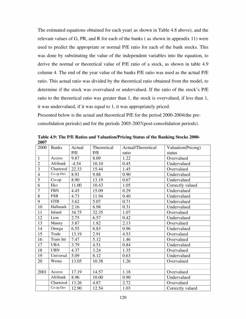
120
The estimated equations obtained for each year( as shown in Table 4.8 above), and the
relevant values of G, PR, and R for each of the banks ( as shown in appendix 11) were
used to predict the appropriate or normal P/E ratio for each of the bank stocks. This
was done by substituting the value of the independent variables into the equation, to
derive the normal or theoretical value of P/E ratio of a stock, as shown in table 4.9
column 4. The end of the year value of the banks P/E ratio was used as the actual P/E
ratio. This actual ratio was divided by the theoretical ratio obtained from the model, to
determine if the stock was overvalued or undervalued. If the ratio of the stock’s P/E
ratio to the theoretical ratio was greater than 1, the stock is overvalued, if less than 1,
it was undervalued, if it was equal to 1, it was appropriately priced.
Presented below is the actual and theoretical P/E for the period 2000-2004(the pre-
consolidation periods) and for the periods 2005-2007(post-consolidation periods).
Table 4.9: The P/E Ratios and Valuation/Pricing Status of the Banking Stocks 2000-2007 2000 Banks Actual
P/E Theoretical P/E
Actual/Theoretical ratio
Valuation(Pricing) status
1 Access 9.87 8.09 1.22 Overvalued 2 Afribank -4.54 10.10 0.45 Undervalued 3 Chartered 22.33 15.44 1.45 Overvalued 4 Co-op Dev 8.91 9.88 0.90 Undervalued 5 Co-op 8.90 13.19 0.67 Undervalued 6 Eko 11.00 10.43 1.05 Correctly valued 7 FBN 4.45 15.09 0.29 Undervalued 8 FSB 4.73 11.94 0.40 Undervalued 9 GTB 3.62 5.07 0.71 Undervalued 10 Hallmark 2.16 6.98 0.31 Undervalued 11 Inland 34.75 32.35 1.07 Overvalued 12 Lion 2.75 6.57 0.42 Undervalued 13 Manny 3.87 1.82 2.13 Overvalued 14 Omega 6.55 6.83 0.96 Undervalued 15 Trade 13.19 2.91 4.53 Overvalued 16 Trans Int 7.47 5.12 1.46 Overvalued 17 UBA 3.79 4.51 0.84 Undervalued 18 UBN 4.37 3.24 1.35 Overvalued 19 Universal 5.09 8.12 0.63 Undervalued 20 Wema 13.05 10.38 1.26 Overvalued 2001 Access 17.19 14.57 1.18 Overvalued Afribank 8.96 10.00 0.90 Undervalued Chartered 13.26 4.87 2.72 Overvalued Co-op Dev 12.90 12.54 1.03 Correctly valued
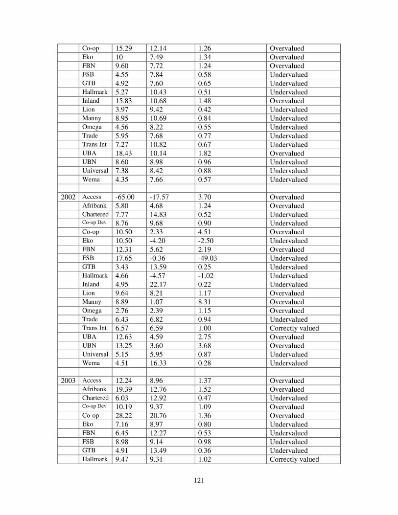
121
Co-op 15.29 12.14 1.26 Overvalued Eko 10 7.49 1.34 Overvalued FBN 9.60 7.72 1.24 Overvalued FSB 4.55 7.84 0.58 Undervalued GTB 4.92 7.60 0.65 Undervalued Hallmark 5.27 10.43 0.51 Undervalued Inland 15.83 10.68 1.48 Overvalued Lion 3.97 9.42 0.42 Undervalued Manny 8.95 10.69 0.84 Undervalued Omega 4.56 8.22 0.55 Undervalued Trade 5.95 7.68 0.77 Undervalued Trans Int 7.27 10.82 0.67 Undervalued UBA 18.43 10.14 1.82 Overvalued UBN 8.60 8.98 0.96 Undervalued Universal 7.38 8.42 0.88 Undervalued Wema 4.35 7.66 0.57 Undervalued 2002 Access -65.00 -17.57 3.70 Overvalued Afribank 5.80 4.68 1.24 Overvalued Chartered 7.77 14.83 0.52 Undervalued Co-op Dev 8.76 9.68 0.90 Undervalued Co-op 10.50 2.33 4.51 Overvalued Eko 10.50 -4.20 -2.50 Undervalued FBN 12.31 5.62 2.19 Overvalued FSB 17.65 -0.36 -49.03 Undervalued GTB 3.43 13.59 0.25 Undervalued Hallmark 4.66 -4.57 -1.02 Undervalued Inland 4.95 22.17 0.22 Undervalued Lion 9.64 8.21 1.17 Overvalued Manny 8.89 1.07 8.31 Overvalued Omega 2.76 2.39 1.15 Overvalued Trade 6.43 6.82 0.94 Undervalued Trans Int 6.57 6.59 1.00 Correctly valued UBA 12.63 4.59 2.75 Overvalued UBN 13.25 3.60 3.68 Overvalued Universal 5.15 5.95 0.87 Undervalued Wema 4.51 16.33 0.28 Undervalued 2003 Access 12.24 8.96 1.37 Overvalued Afribank 19.39 12.76 1.52 Overvalued Chartered 6.03 12.92 0.47 Undervalued Co-op Dev 10.19 9.37 1.09 Overvalued Co-op 28.22 20.76 1.36 Overvalued Eko 7.16 8.97 0.80 Undervalued FBN 6.45 12.27 0.53 Undervalued FSB 8.98 9.14 0.98 Undervalued GTB 4.91 13.49 0.36 Undervalued Hallmark 9.47 9.31 1.02 Correctly valued
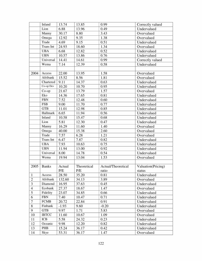
122
Inland 13.74 13.85 0.99 Correctly valued Lion 6.88 13.96 0.49 Undervalued Manny 30.17 8.80 3.43 Overvalued Omega 12.92 9.35 1.38 Overvalued Trade 4.69 9.15 0.51 Undervalued Trans Int 24.93 18.60 1.34 Overvalued UBA 6.68 12.82 0.52 Undervalued UBN 10.57 13.86 0.76 Undervalued Universal 14.41 14.61 0.99 Correctly valued Wema 7.14 12.39 0.58 Undervalued 2004 Access 22.00 13.95 1.58 Overvalued Afribank 15.52 8.56 1.81 Overvalued Chartered 9.11 14.37 0.63 Undervalued Co-op Dev 10.20 10.70 0.95 Undervalued Co-op 21.67 13.79 1.57 Overvalued Eko 14.36 17.65 0.81 Undervalued FBN 7.52 12.48 0.60 Undervalued FSB 9.00 11.70 0.77 Undervalued GTB 11.01 12.98 0.85 Undervalued Hallmark 6.65 11.94 0.56 Undervalued Inland 10.58 15.47 0.68 Undervalued Lion 5.81 12.30 0.47 Undervalued Manny 16.29 11.60 1.40 Overvalued Omega 40.00 15.38 2.60 Overvalued Trade 7.57 6.28 1.21 Overvalued Trans Int 6.47 7.87 0.82 Undervalued UBA 7.93 10.63 0.75 Undervalued UBN 11.94 13.00 0.92 Undervalued Universal 8.00 14.78 0.54 Undervalued Wema 19.94 13.04 1.53 Overvalued 2005 Banks Actual
P/E Theoretical P/E
Actual/Theoretical ratio
Valuation(Pricing) status
1 Access 28.50 35.20 0.81 Undervalued 2 Afribank 132.60 34.13 3.89 Overvalued 3 Diamond 16.95 37.63 0.45 Undervalued 4 Ecobank 27.37 18.67 1.47 Overvalued 5 Fidelity 23.07 34.85 0.66 Undervalued 6 FBN 7.40 10.47 0.71 Undervalued 7 FCMB 20.72 22.84 0.91 Undervalued 8 Finbank -1.93 9.60 -0.20 Undervalued 9 GTB 9.97 1.71 5.83 Overvalued 10 IBTCC 11.60 10.67 1.09 Overvalued 11 ICB 5.58 24.32 0.23 Undervalued 12 Oceanic 9.98 12.20 0.82 Undervalued 13 PHB 15.24 36.17 0.42 Undervalued 14 Skye 53.31 36.17 1.47 Overvalued
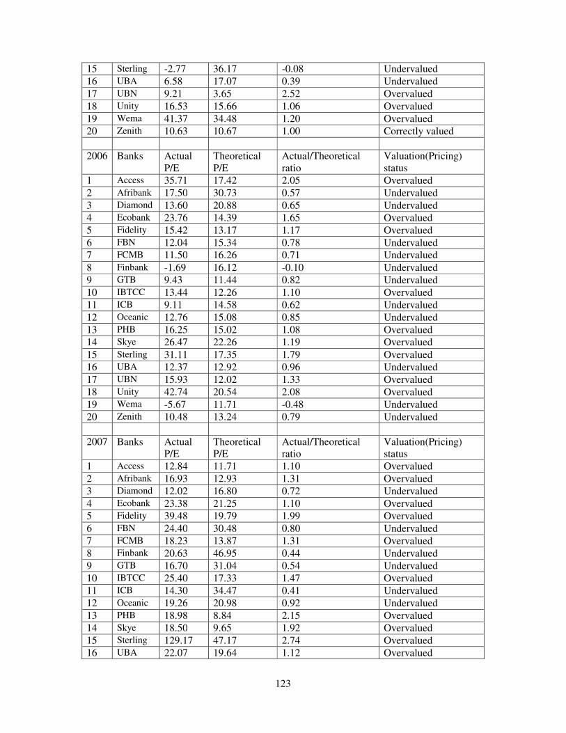
123
15 Sterling -2.77 36.17 -0.08 Undervalued 16 UBA 6.58 17.07 0.39 Undervalued 17 UBN 9.21 3.65 2.52 Overvalued 18 Unity 16.53 15.66 1.06 Overvalued 19 Wema 41.37 34.48 1.20 Overvalued 20 Zenith 10.63 10.67 1.00 Correctly valued 2006 Banks Actual
P/E Theoretical P/E
Actual/Theoretical ratio
Valuation(Pricing) status
1 Access 35.71 17.42 2.05 Overvalued 2 Afribank 17.50 30.73 0.57 Undervalued 3 Diamond 13.60 20.88 0.65 Undervalued 4 Ecobank 23.76 14.39 1.65 Overvalued 5 Fidelity 15.42 13.17 1.17 Overvalued 6 FBN 12.04 15.34 0.78 Undervalued 7 FCMB 11.50 16.26 0.71 Undervalued 8 Finbank -1.69 16.12 -0.10 Undervalued 9 GTB 9.43 11.44 0.82 Undervalued 10 IBTCC 13.44 12.26 1.10 Overvalued 11 ICB 9.11 14.58 0.62 Undervalued 12 Oceanic 12.76 15.08 0.85 Undervalued 13 PHB 16.25 15.02 1.08 Overvalued 14 Skye 26.47 22.26 1.19 Overvalued 15 Sterling 31.11 17.35 1.79 Overvalued 16 UBA 12.37 12.92 0.96 Undervalued 17 UBN 15.93 12.02 1.33 Overvalued 18 Unity 42.74 20.54 2.08 Overvalued 19 Wema -5.67 11.71 -0.48 Undervalued 20 Zenith 10.48 13.24 0.79 Undervalued 2007 Banks Actual
P/E Theoretical P/E
Actual/Theoretical ratio
Valuation(Pricing) status
1 Access 12.84 11.71 1.10 Overvalued 2 Afribank 16.93 12.93 1.31 Overvalued 3 Diamond 12.02 16.80 0.72 Undervalued 4 Ecobank 23.38 21.25 1.10 Overvalued 5 Fidelity 39.48 19.79 1.99 Overvalued 6 FBN 24.40 30.48 0.80 Undervalued 7 FCMB 18.23 13.87 1.31 Overvalued 8 Finbank 20.63 46.95 0.44 Undervalued 9 GTB 16.70 31.04 0.54 Undervalued 10 IBTCC 25.40 17.33 1.47 Overvalued 11 ICB 14.30 34.47 0.41 Undervalued 12 Oceanic 19.26 20.98 0.92 Undervalued 13 PHB 18.98 8.84 2.15 Overvalued 14 Skye 18.50 9.65 1.92 Overvalued 15 Sterling 129.17 47.17 2.74 Overvalued 16 UBA 22.07 19.64 1.12 Overvalued
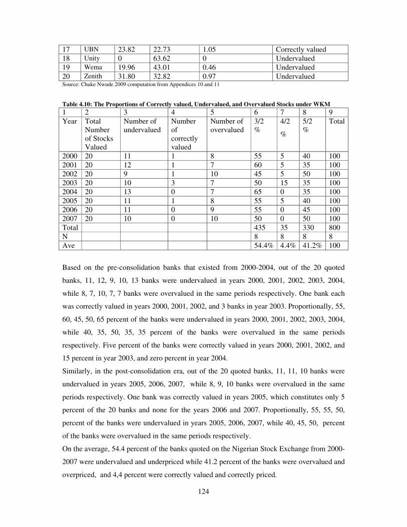
124
17 UBN 23.82 22.73 1.05 Correctly valued 18 Unity 0 63.62 0 Undervalued 19 Wema 19.96 43.01 0.46 Undervalued 20 Zenith 31.80 32.82 0.97 Undervalued Source: Chuke Nwude 2009 computation from Appendices 10 and 11
Table 4.10: The Proportions of Correctly valued, Undervalued, and Overvalued Stocks under WKM 1 2 3 4 5 6 7 8 9 Year Total
Number of Stocks Valued
Number of undervalued
Number of correctly valued
Number of overvalued
3/2 %
4/2
%
5/2 %
Total
2000 20 11 1 8 55 5 40 100 2001 20 12 1 7 60 5 35 100 2002 20 9 1 10 45 5 50 100 2003 20 10 3 7 50 15 35 100 2004 20 13 0 7 65 0 35 100 2005 20 11 1 8 55 5 40 100 2006 20 11 0 9 55 0 45 100 2007 20 10 0 10 50 0 50 100 Total 435 35 330 800 N 8 8 8 8 Ave 54.4% 4.4% 41.2% 100
Based on the pre-consolidation banks that existed from 2000-2004, out of the 20 quoted
banks, 11, 12, 9, 10, 13 banks were undervalued in years 2000, 2001, 2002, 2003, 2004,
while 8, 7, 10, 7, 7 banks were overvalued in the same periods respectively. One bank each
was correctly valued in years 2000, 2001, 2002, and 3 banks in year 2003. Proportionally, 55,
60, 45, 50, 65 percent of the banks were undervalued in years 2000, 2001, 2002, 2003, 2004,
while 40, 35, 50, 35, 35 percent of the banks were overvalued in the same periods
respectively. Five percent of the banks were correctly valued in years 2000, 2001, 2002, and
15 percent in year 2003, and zero percent in year 2004.
Similarly, in the post-consolidation era, out of the 20 quoted banks, 11, 11, 10 banks were
undervalued in years 2005, 2006, 2007, while 8, 9, 10 banks were overvalued in the same
periods respectively. One bank was correctly valued in years 2005, which constitutes only 5
percent of the 20 banks and none for the years 2006 and 2007. Proportionally, 55, 55, 50,
percent of the banks were undervalued in years 2005, 2006, 2007, while 40, 45, 50, percent
of the banks were overvalued in the same periods respectively.
On the average, 54.4 percent of the banks quoted on the Nigerian Stock Exchange from 2000-
2007 were undervalued and underpriced while 41.2 percent of the banks were overvalued and
overpriced, and 4,4 percent were correctly valued and correctly priced.
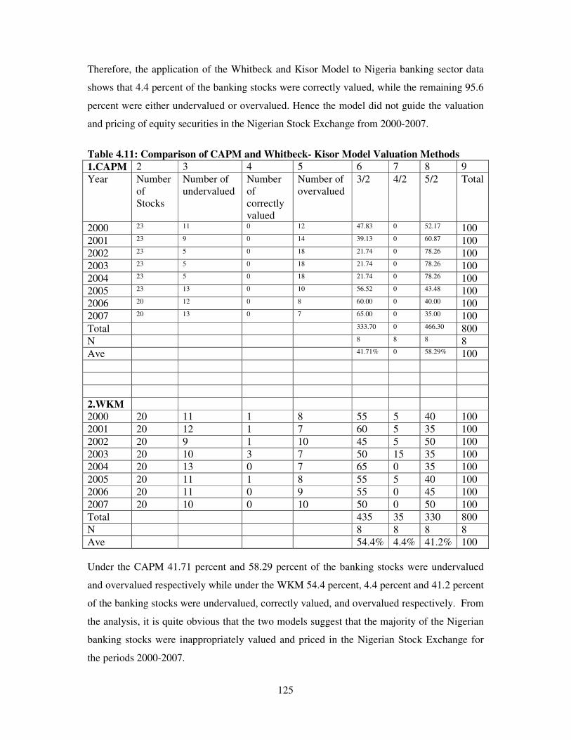
125
Therefore, the application of the Whitbeck and Kisor Model to Nigeria banking sector data
shows that 4.4 percent of the banking stocks were correctly valued, while the remaining 95.6
percent were either undervalued or overvalued. Hence the model did not guide the valuation
and pricing of equity securities in the Nigerian Stock Exchange from 2000-2007.
Table 4.11: Comparison of CAPM and Whitbeck- Kisor Model Valuation Methods 1.CAPM 2 3 4 5 6 7 8 9 Year Number
of Stocks
Number of undervalued
Number of correctly valued
Number of overvalued
3/2 4/2 5/2 Total
2000 23 11 0 12 47.83 0 52.17 100 2001 23 9 0 14 39.13 0 60.87 100 2002 23 5 0 18 21.74 0 78.26 100 2003 23 5 0 18 21.74 0 78.26 100 2004 23 5 0 18 21.74 0 78.26 100 2005 23 13 0 10 56.52 0 43.48 100 2006 20 12 0 8 60.00 0 40.00 100 2007 20 13 0 7 65.00 0 35.00 100 Total 333.70 0 466.30 800 N 8 8 8 8 Ave 41.71% 0 58.29% 100 2.WKM 2000 20 11 1 8 55 5 40 100 2001 20 12 1 7 60 5 35 100 2002 20 9 1 10 45 5 50 100 2003 20 10 3 7 50 15 35 100 2004 20 13 0 7 65 0 35 100 2005 20 11 1 8 55 5 40 100 2006 20 11 0 9 55 0 45 100 2007 20 10 0 10 50 0 50 100 Total 435 35 330 800 N 8 8 8 8 Ave 54.4% 4.4% 41.2% 100 Under the CAPM 41.71 percent and 58.29 percent of the banking stocks were undervalued
and overvalued respectively while under the WKM 54.4 percent, 4.4 percent and 41.2 percent
of the banking stocks were undervalued, correctly valued, and overvalued respectively. From
the analysis, it is quite obvious that the two models suggest that the majority of the Nigerian
banking stocks were inappropriately valued and priced in the Nigerian Stock Exchange for
the periods 2000-2007.
126
4.3 Test of the Hypotheses
To achieve the objectives of the study, following propositions were formulated for the study.
HO1: From the perspective of the required and actual rates of return, the subject-banks
stocks
were not correctly valued by the market.
On the average, 34.78% of the banking stocks were undervalued, and 65.22% overvalued
during the pre-consolidation era while 62.50% were undervalued, and 37.50% overvalued in
post-consolidation banks, within the period under study. There was not, a single correctly
valued stock within the period under study. Therefore, the application of the Capital Asset
Pricing Model to Nigeria banking sector data shows that zero percent of the banking stocks
were correctly valued, while 100 percent were either undervalued or overvalued. Hence the
model did not guide the valuation and pricing of equity securities in the Nigerian Stock
Exchange from 2000-2007.
HO2: From the perspective of the Price-Earnings multiple, the subject-banks stocks were not
correctly priced by the market.
In year 2000, 66.1% of variations in PE were explained by the predictors. A high F-value of
13.342 compared against its table value of 6.30 and a significance of 0.000 shows that there
was a significant relationship between the dependent and independent variables. The DW
value of 2.454 shows this result was within the acceptable region, implying the absence of
any serial auto-correlation. Considering the t value 2.180 > 2.0, it can be further established
that the variables fit into the model, though R has a weak negative correlation with PE
(having a coefficient of -0.231). Therefore, the null hypothesis should be rejected while the
alternate accepted.
In year 2001, 23.2% of variations in PE were explained by the predictors. A low F-value of
1.614 compared against its table value of 6.30 and a significance of 0.225 being higher than
the critical value of 0.025 (2-tailed) shows that there was no significant relationship between
the dependent and independent variables. The DW value of 2.154 shows this result was
within the acceptable region, implying the absence of any serial auto-correlation. Considering
the t value 3.819 > 2.0, it can be further established that the variables fit into the model,
127
though all the independent variables have little or no correlation with PE. Therefore, the null
hypothesis should be accepted.
In year 2002, 26.5% of variations in PE were explained by the predicators. A low F-value of
1.926 compared against its table value of 6.30 and a significance of 0.166 being higher than
the critical value of 0.025 (2-tailed) shows that there was no significant relationship between
the dependent and independent variables. The DW value of 1.492 shows this result was
within the acceptable region, implying the absence of any serial auto-correlation. Considering
the regression coefficient (r) = 0.515 implying an average correlation, it can be established
that the variables fit into the model, though all the independent variables have little or no
correlation with PE. Therefore, the null hypothesis should be accepted.
In year 2003, 18.3% of variations in PE were explained by the predicators. A low F-value of
1.198 compared against its table value of 6.30 and a significance of 0.342 being higher than
the critical value of 0.025 (2-tailed) shows that there was no significant relationship between
the dependent and independent variables. The DW value of 2.3044 shows this result is within
the acceptable region, implying the absence of any serial auto-correlation. Considering the t
value 2.459 > 2.0, it can be further established that the variables fit into the model, though all
the independent variables have little or no correlation with PE. Therefore, the null hypothesis
should be accepted.
In year 2004, 15.6% of variations in PE were explained by the predicators. A low F-value of
0.983 compared against its table value of 6.30 and a significance of 0.45 being higher than
the critical value of 0.025 (2-tailed) shows that there was no significant relationship between
the dependent and independent variables. The DW value of 1.470 shows this result is within
the acceptable region, implying the absence of any serial auto-correlation. Considering the t
value 3.024 > 2.0, it can be further established that the variables fit into the model, though all
the independent variables have little or no correlation with PE. Therefore, the null hypothesis
should be accepted.
In year 2005, 18.1% of variations in PE were explained by the predicators. A low F-value of
1.182 compared against its table value of 6.30 and a significance of 0.348 being lower than
the critical value of 0.025 (2-tailed) shows that there was no significant relationship between
the dependent and independent variables. The DW value of 2.533 shows this result is within

128
the acceptable region, implying the absence of any serial auto-correlation. Considering the t
value 3.503 > 2.0, it can be further established that the variables fit into the model, though all
the independent variables have little or no correlation with PE. Therefore, the null hypothesis
should be accepted.
In year 2006, 16.6% of variations in PE were explained by the predicators. A low F-value of
1.059 compared against its table value of 6.30 and a significance of 0.394 being lower than
the critical value of 0.025 (2-tailed) shows that there was no significant relationship between
the dependent and independent variables. The DW value of 2.087 shows this result is within
the acceptable region, implying the absence of any serial auto-correlation. Considering the t
value 3.279 > 2.0, it can be further established that the variables fit into the model, though all
the independent variables have little or no correlation with PE. Therefore, the null hypothesis
should be accepted.
In year 2007, 20.4% of variations in PE were explained by the predicators. A low F-value of
1.365 compared against its table value of 6.30 and a significance of 0.289 being lower than
the critical value of 0.025 (2-tailed) shows that there is no significant relationship between
the dependent and independent variables. The DW value of 1.831 shows this result is within
the acceptable region, implying the absence of any serial auto-correlation. Considering the t
value 3.023 > 2.0, it can be further established that the variables fit into the model, though all
the independent variables have little or no correlation with PE. Therefore, the null hypothesis
should be accepted.
Therefore, the model did not guide the valuation and pricing of equity securities in the
Nigerian Stock Exchange from 2000-2007.
HO3: None of the valuation models guides the valuation and pricing of ordinary shares of
the subject-banks in the Nigerian stock exchange.
Under the CAPM, 41.71 percent and 58.29 percent of the banking stocks were undervalued
and overvalued respectively while under the WKM 54.4 percent, 4.4 percent and 41.2 percent
of the banking stocks were undervalued, correctly valued, and overvalued respectively. From
the analysis, it is quite obvious that none of the valuation models guided the valuation and
pricing of ordinary shares of the subject-banks in the Nigerian Stock Exchange for the
periods 2000-2007.

129
CHAPTER FIVE
SUMMARY OF FINDINGS, CONCLUSIONS AND RECOMMENDATIONS
5.0 Introduction
This chapter presents the summary of findings of this research work. It also shows the
conclusions drawn from the study and the recommendations made.
5.1 Summary of Findings
This study examined the appropriateness of valuation and pricing of securities in Nigerian
Stock Exchange with reference to banking stocks. Banks, as we know, are the major
financiers of economic activities in other sectors of any economy. The sample of study is all
the quoted banks on the Nigerian Stock Exchange as they dominate the activities in the
market in terms of volume of shares traded and market capitalization. Three hypotheses were
proposed and tested to explain the mechanics of valuation and pricing of ordinary shares in
the market. Two valuation methods which appeared to be popular among researchers in
equity securities valuation were used. The two principal paradigms that are popular are the
Capital Asset Pricing Model (CAPM) as developed by Sharpe (1964) supported by Lintner
(1965) and Mossin (1966), and the Whitbeck - Kisor Model (WKM) as developed by
Whitbeck and Kisor (1963).
Data for this research were collected mainly from secondary sources-audited annual reports
of sampled banks, periodicals, various publications of Central Bank of Nigeria annual reports
and statistical bulletins, Daily official lists and statistical year books of Nigerian Stock

130
Exchange, different publications of Securities and Exchange Commission and Nigerian
Deposit Insurance Corporation, and the internet. All the 23 pre-consolidation and 20 out of
the 21 post-consolidation quoted banks were used for the study. The study covered an eight
year period (2000-2007), pre and post bank consolidation periods.
In line with previous similar studies on equity securities valuation, the expected and actual
returns, multiple linear regression model, and Pearson product moment correlation coefficient
were employed to determine the valuation status of the equity securities based on return
generating capacity of each equity. The SPSS version 13.0 as a computer program was used
for the analyses.
Under the two methods of valuation, it is assumed that while markets may make mistakes on
how they price individual stocks, they are correct on average. Hence we value an asset based
upon how similar assets are priced and this is termed relative valuation. Relative valuation is
built on standardized prices upon which market value is scaled to some common measure
such as earnings, book value or revenues. It is the dominant valuation approach in practice
and being an empirical study, analytical research design was adopted.
Within the period under study (2000-2007) the following observations were made by the
researcher. 1. The Nigerian stock market was subjected to waves of optimistic and
pessimistic sentiments even when no objective evidence existed for such sentiments. The
stock price movements were caused largely by changes in the perception of ignorant
speculators, tinted with a significant degree of order and coherence infused by the
institutional and social structures. The only memory stock price has is the 5% margin of price
increase or decrease on each day trading.
2. The political developments in Nigeria such as the level of confidence in the government,
the climate of stability in policies and programs of government (the no-shaky posture of the
Obasanjo-led government in power) impacted positively on share prices. 3.Margin account
borrowing as offered by banks and other financial institutions became the order of the day
and this created the needed liquidity in the stock market. Consequently a large amount of
money was chasing limited available shares of companies that were doing well. As demand
for the shares exceeded the supply, share prices were sent to the high levels. When the shares
of the blue-chip companies were cleared up in the market, investors then descended on penny

131
stocks just to create market for them and do away with idle cash. This automatically inflamed
the stock market with rising share prices across the board, even among dying companies.
Doctored financial news as published by the banks with quoted shares, with respect to EPS,
DPS, capital appreciation, acquisition of foreign technical partners, foreign investors
involvement, opening of foreign subsidiaries(which became a status symbol), acquisition of
junior banks in the system, level of deposit mobilized, gross earnings, profit before and after
tax, staff salary package, posh offices and posh cars, big ticket transactions, investment in oil
and gas, etc constitute the trend upon which the likely trend in future price per share was
determined. It was only the benchmark of plus or minus 5% increase or decrease in share
price over the previous day’s trading price that guided the direction of the future share price
for the next trading day.
In Nigeria, majority of investors are carried away with the dreams of immediate wealth in
share investment. Many people see others getting rich quick through share investment and
their need to be wealthy. As a result of this way of thinking, the investing public went wild
pumping money into investment in shares. This of course created massive chase for the
limited available shares in the market. As demand for the limited available shares exceeds
supply, massive run-up in the share prices ensued, which sends stock prices soaring high.
This process continued until the economic realities of the companies are left far behind.
Within the period of study, the findings were as follows:
It was observed in this study that share prices respond to newly released information relating
to the company involved but the speed at which the market assimilate such information could
not be ascertained. Again such information was being made available on time to the very few
privileged investors(speculators) who act on it earlier before it is made available to the
general public(insider information). Hence the Nigerian stock market is a weak-efficient form
of stock market. In operational efficient stock market, the timing of new issues of equity is
immaterial and uncontrolled because the price payable for the new equity will always be a
fair one. But the Nigerian stock market is operationally inefficient because the new issues of
equity is controlled and most often issued at an unfair offer price.
While Rozett and Kinney (1976), Bhwardwaj and Brooks (1992), Reinganum (1993), noted
that on the average, the returns from the stocks were higher for the month of January

132
compared to the other months. In this study it was discovered that the returns from the stocks
were higher for the month of February compared to the other months. February produced
highest return 19 times, January (14 times), August (7 times), June and September (6 times)
each, July, October-December(5 times) each, March, April, May(4 times). This confirms the
existence of February effect in the Nigerian stock market.
As documented by French (1980), Lakonishok and Maberly (1990), Agrawal and Tandon
(1994), returns tend to be low on Mondays whereas they are relatively high on the other days
of the week. This situation is believed to be caused by weekend expenditure effect. It serves
as a pointer that for an investor to trade profitably, he should adopt the strategy of buying on
Mondays and selling them on Fridays. Hence there exists Weekend or Monday effect in
Nigerian Stock Market.
It was discovered that stock prices/returns are higher on the last five and first three trading
days of the month in the market thereby supporting the views of Cadsby and Ratner (1992),
Haugen and Lakonishok (1998) and Ariel (1987) on the turn of the month effect on stock
markets in USA, UK, France and Japan.
On the average, stock prices are higher three days before a holiday and lower five days after
the holiday. This indicates pre and post holiday effects on the stock prices. This is because
people cut short their investment in shares and even offload some in order to create cash they
will use during the holiday and few days after the holiday period. The same thing applies
during festival periods like Muslim and Christian festivals. This is termed the festival effect.
There are strong demands for penny stocks (that is low capitalization companies) because
they provide excess returns better than highly capitalized companies. This rush to buy the
penny stocks causes their demand to exceed their supply thereby causing a massive run-up on
their share prices, even beyond what the fundamentals of the companies could support. As a
result, higher returns were earned by holding the stocks of low capitalized companies than
that from highly capitalized companies. This is called small-size-firms effect as also observed
by Banz (1981) and Reinganum (1983).

133
Short-sellers (the speculators) position themselves in stocks of firms with low P/E ratios and
obtained a high future returns in terms of dividend income and price appreciation, thereby
supporting the findings of Basu (1977), Dechow, Hutton and Sloan (1999).
There was astronomical increase in share price on the announcement of inclusion of a stock
into the list of quoted companies on the Nigerian stock exchange (The NSE). Evidence
includes Dangote Sugar quoted at N15.00 but went up to N64.00, Dangote Flour quoted at
N18.00 but went up to N57.00, Tantalizers quoted at N2.50 but went up to N7.00, Fidson
quoted at N6.50 but went up to N15.00, Fidelity bank quoted at N2.50 but went up to N14.00,
Diamond bank quoted at N5.00 but went up to N28.00, and many others within one year(NSE
Daily Official Lists). The study is termed The NSE effect.
Nigerian banks made wide and loud publicity of earnings on popular news media and internet
and this generated over reaction of investors especially on positive changes in current
earnings, not minding that some of the accounting incomes were doctored. This supports the
view of Huberman and Regeve (2001).
Trend chasing and tracking of possible indicators of demand which constitute noise rather
than rational evaluation of information are the order of the day. Investors’ sentiments move
prices and so predicting changes in the sentiments pays. This is termed follow the crowd or
social fads with very little rational or logical explanations.
The influence of weather was noticed in the choices and judgements of investors who
engaged in agriculture. This type of hybrid investors usually divest some of their
shareholdings prior to farming season in order to enable them make purchases of farm needs
ahead of farming period. Massive offload of their shareholdings created excess supply which
usually caused price decline, especially when the supply exceeded demand. They also
invested heavily with their farm proceeds during harvesting period, thereby causing rise in
prices, especially when the demand exceeded supply. This type of investors is noise traders
who trade on the basis of imperfect information. The imperfect information causes share
prices to deviate from equilibrium values. In a situation like this, share prices do not merely
respond to information but also to changes in expectations or sentiments which are not fully
justified.

134
The application of the capital asset pricing model (CAPM) to Nigeria banking sector data
shows that on the average, 34.78% of the banking stocks were undervalued, and 65.22%
overvalued during the pre-consolidation era while 62.50% were undervalued, and 37.50%
overvalued in post-consolidation banks, within the period under study. There was not, a
single correctly valued stock within the period under study. Therefore, the application of the
Capital Asset Pricing Model to Nigeria banking sector data shows that 100 percent of the
banking stocks were either undervalued or overvalued while zero percent of the banking
stocks were correctly valued. Hence the model did not guide the valuation and pricing of
equity securities in the Nigerian Stock Exchange from 2000-2007.
The application of the Whitbeck-Kisor Model(WKM) to Nigeria banking sector data shows
that on the average, 54.4 percent of the banks quoted on the Nigerian Stock Exchange from
2000-2007 were undervalued and underpriced while 41.2 percent of the banks were
overvalued and overpriced, and 4,4 percent were correctly valued and correctly priced.
Therefore, the application of the Whitbeck and Kisor Model to Nigeria banking sector data
shows that 4.4 percent of the banking stocks were correctly valued, while the remaining 95.6
percent were either undervalued or overvalued. Hence the model did not guide the valuation
and pricing of equity securities in the Nigerian Stock Exchange from 2000-2007.
The cross-sectional multiple regressions carried out on the quoted banks making up the
banking sector produced the predictive equations in table 4.8 in chapter four, page 120. These
equations deviated from the one obtained by WKM in the developed market, in terms of signs
(direction) and magnitude of the coefficients. The positive coefficients indicate that there was
positive correlation between the variable and the P/E ratio. The negative coefficients indicate
that there was negative correlation between the variable and the P/E ratio.In the work of
WKM earnings growth rate and the dividend payout ratio were positively correlated to P/E
ratio while the risk was negatively correlated to the P/E ratio. In terms of sign, only year 2002
equation had the same type of correlation as that of the WKM.
The pre consolidation banks’ expected growth rate in earnings (g), dividend payout ratio (p),
and risk(r) also had marginal relationship with the P/E ratios but the moment the
consolidation exercise was announced on July 6, 2004, emphasis shifted from the banks’
expected growth rate in earnings (g), dividend payout ratio (p), and risk (r) to which bank will
survive the exercise. As the emphasis on the banks’ expected growth rate in earnings (g),
135
dividend payout ratio (p), and risk (r) backslided from 2004 (when the consolidation was
kicked up) the g, p, and r had weak relationship with the P/E ratios as can be noted in table
above. Consequently, especially in 2007, stock pricing was based on such investors’
psychology and nothing more. For 2006, the euphoria of getting rich quick through
investment in shares caught up with everyone and as demand for shares exceeded supply, the
price went haywire paying little attention to the fundamental determinants like the banks’
expected growth rate in earnings (g), expected dividend payout ratio (p), and risk (r).
In year 2000, 66.1% of variations in PE were explained by the predictors. A high F-value of
13.342 compared against its table value of 6.30 and a significance of 0.000 shows that there
was a significant relationship between the dependent and independent variables. The DW
value of 2.454 shows this result was within the acceptable region, implying the absence of
any serial auto-correlation. Considering the t value 2.180 > 2.0, it can be further established
that the variables fit into the model, though R has a weak negative correlation with PE
(having a coefficient of -0.231). Therefore, the null hypothesis should be rejected while the
alternate accepted.
In year 2001, 23.2% of variations in PE were explained by the predictors. A low F-value of
1.614 compared against its table value of 6.30 and a significance of 0.225 being higher than
the critical value of 0.025 (2-tailed) shows that there was no significant relationship between
the dependent and independent variables. The DW value of 2.154 shows this result was
within the acceptable region, implying the absence of any serial auto-correlation. Considering
the t value 3.819 > 2.0, it can be further established that the variables fit into the model,
though all the independent variables have little or no correlation with PE. Therefore, the null
hypothesis should be accepted.
In year 2002, 26.5% of variations in PE were explained by the predicators. A low F-value of
1.926 compared against its table value of 6.30 and a significance of 0.166 being higher than
the critical value of 0.025 (2-tailed) shows that there was no significant relationship between
the dependent and independent variables. The DW value of 1.492 shows this result was
within the acceptable region, implying the absence of any serial auto-correlation. Considering
the regression coefficient (r) = 0.515 implying an average correlation, it can be established
136
that the variables fit into the model, though all the independent variables have little or no
correlation with PE. Therefore, the null hypothesis should be accepted.
In year 2003, 18.3% of variations in PE were explained by the predicators. A low F-value of
1.198 compared against its table value of 6.30 and a significance of 0.342 being higher than
the critical value of 0.025 (2-tailed) shows that there was no significant relationship between
the dependent and independent variables. The DW value of 2.3044 shows this result is within
the acceptable region, implying the absence of any serial auto-correlation. Considering the t
value 2.459 > 2.0, it can be further established that the variables fit into the model, though all
the independent variables have little or no correlation with PE. Therefore, the null hypothesis
should be accepted.
In year 2004, 15.6% of variations in PE were explained by the predicators. A low F-value of
0.983 compared against its table value of 6.30 and a significance of 0.45 being higher than
the critical value of 0.025 (2-tailed) shows that there was no significant relationship between
the dependent and independent variables. The DW value of 1.470 shows this result is within
the acceptable region, implying the absence of any serial auto-correlation. Considering the t
value 3.024 > 2.0, it can be further established that the variables fit into the model, though all
the independent variables have little or no correlation with PE. Therefore, the null hypothesis
should be accepted.
In year 2005, 18.1% of variations in PE were explained by the predicators. A low F-value of
1.182 compared against its table value of 6.30 and a significance of 0.348 being lower than
the critical value of 0.025 (2-tailed) shows that there was no significant relationship between
the dependent and independent variables. The DW value of 2.533 shows this result is within
the acceptable region, implying the absence of any serial auto-correlation. Considering the t
value 3.503 > 2.0, it can be further established that the variables fit into the model, though all
the independent variables have little or no correlation with PE. Therefore, the null hypothesis
should be accepted.
In year 2006, 16.6% of variations in PE were explained by the predicators. A low F-value of
1.059 compared against its table value of 6.30 and a significance of 0.394 being lower than
the critical value of 0.025 (2-tailed) shows that there was no significant relationship between
the dependent and independent variables. The DW value of 2.087 shows this result is within
137
the acceptable region, implying the absence of any serial auto-correlation. Considering the t
value 3.279 > 2.0, it can be further established that the variables fit into the model, though all
the independent variables have little or no correlation with PE. Therefore, the null hypothesis
should be accepted.
In year 2007, 20.4% of variations in PE were explained by the predicators. A low F-value of
1.365 compared against its table value of 6.30 and a significance of 0.289 being lower than
the critical value of 0.025 (2-tailed) shows that there is no significant relationship between
the dependent and independent variables. The DW value of 1.831 shows this result is within
the acceptable region, implying the absence of any serial auto-correlation. Considering the t
value 3.023 > 2.0, it can be further established that the variables fit into the model, though all
the independent variables have little or no correlation with PE. Therefore, the null hypothesis
should be accepted.
5.2 Conclusions
Based on the major findings of the research a number of conclusions could be made as
follows. The application of the capital asset pricing model(CAPM) to Nigeria banking sector
data shows that on the average, 34.78 percent of the banking stocks quoted on the Nigerian
Stock Exchange were undervalued, and 65.22 percent were overvalued during the pre-
consolidation era while 62.50 percent were undervalued, and 37.50 percent were overvalued
in post-consolidation banks, within the period under study. There was not, a single correctly
valued bank stock over the period. Therefore, the application of the Capital Asset Pricing
Model to Nigeria banking sector data shows that 100 percent of the banking stocks were
either undervalued or overvalued while zero percent of the banking stocks was correctly
valued. Hence the model did not guide the valuation and pricing of equity securities in the
Nigerian Stock Exchange from 2000-2007.
Again the application of the Whitbeck-Kisor Model(WKM) to Nigeria banking sector data
shows that on the average, 54.4 percent of the banks quoted on the Nigerian Stock Exchange
from 2000-2007 were undervalued and underpriced while 41.2 percent of the banks were
overvalued and overpriced, and 4,4 percent were correctly valued and correctly priced.
Therefore, the application of the Whitbeck and Kisor Model to Nigeria banking sector data
shows that 4.4 percent of the banking stocks were correctly valued, while the remaining 95.6
138
percent were either undervalued or overvalued. Hence the model did not guide the valuation
and pricing of equity securities in the Nigerian Stock Exchange from 2000-2007.
When CAPM was applied in the valuation process, 41.71% and 58.29% of the banking
stocks were undervalued and overvalued respectively while under the WKM, 54.4%, 4.4%,
and 41.2% were undervalued, correctly valued, and overvalued respectively. There was no
correctly valued stock based on CAPM pricing. From the analysis, it is quite obvious that the
two models give divergent views on stock valuation. Therefore, it is concluded that none of
the models tested gave a failure proof guide to the valuation and pricing of equity securities
in Nigerian Stock Exchange market. The valuation and pricing of equity securities in
Nigerian Stock market do not appear to be guided by growth rate in earnings, dividend
payout ratio and risk exposure variables.
That Stock prices deviate from their fundamental values as a result of the buy and sell
positions of uninformed investors (noise trading) and the informed investors were willing to
capitalize on the discrepancy. In effect, stock price changes act as though they were
independent random drawings from an infinite pool of possible prices. The only memory
stock price has is the 5% margin of price increase or decrease on each day trading. This is in
line with the empirical evidence from research studies by Fisher and Lorie (1964), Madelbrot
(1963), Fama (1965), Granger and Morgensten (1970) which posit the independence of future
stock price movements from past trends in stock prices.
The Whitbeck and Kisor(1963) regressed P/E ratio against the earnings growth rate(EGR),
dividend payout ratio(POR), and the risk (R) using data from the Bank of New York for 135
stocks to arrive at their own predictive equation for one year. Bower and Bower (1969)
regressed for 1956 – 1964 period and Malkiel and Cragg (1970) regressed for 1961 -1965
period to arrive at their predictive equations for each of the years. The regressions were
updated in Damodaran (1996 and 2002) for the period 1987 – 1991 to generate his own
predictive equations for each of the years 1987 – 1991. All these were carried out on
developed stock market. None was done on a developing stock market like Nigeria.
Therefore the major contribution of this work lies in the geography of the research. Now we
can boast of our own predictive equations for estimating normal P/E ratio for the Nigerian
Banking industry for the period 2000 – 2007, which is a major contribution indeed. The
predictive equations are as shown below.
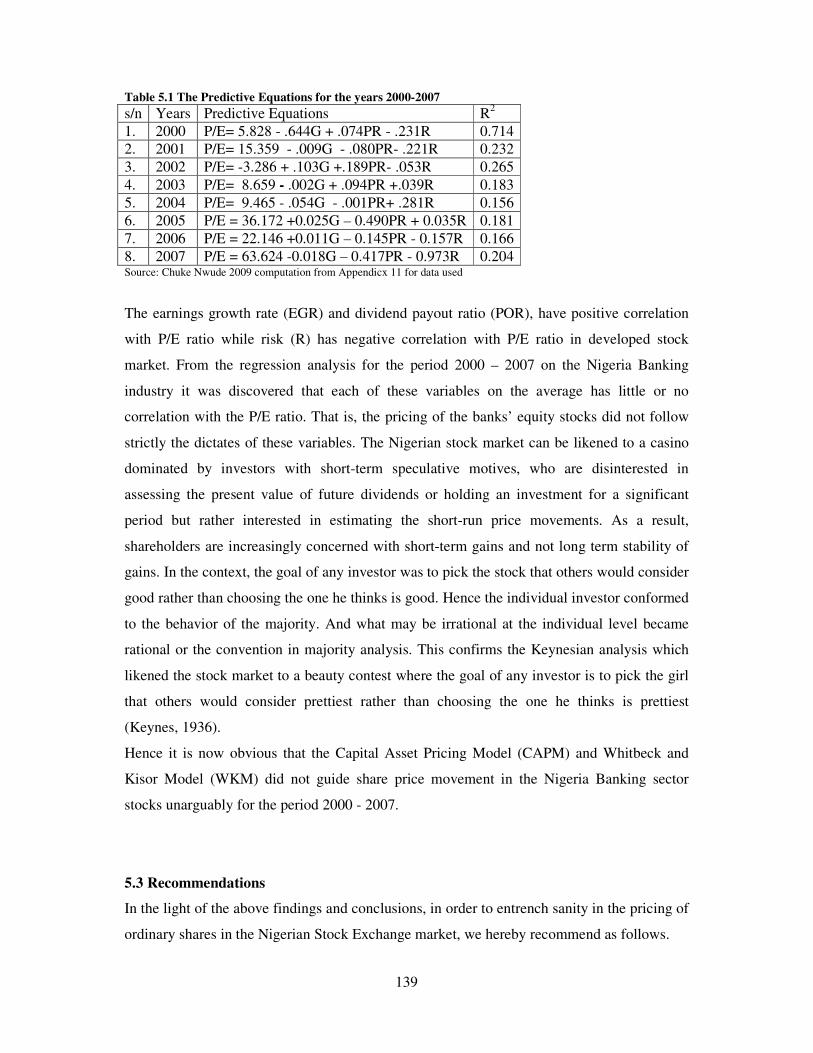
139
Table 5.1 The Predictive Equations for the years 2000-2007 s/n Years Predictive Equations R2 1. 2000 P/E= 5.828 - .644G + .074PR - .231R 0.714 2. 2001 P/E= 15.359 - .009G - .080PR- .221R 0.232 3. 2002 P/E= -3.286 + .103G +.189PR- .053R 0.265 4. 2003 P/E= 8.659 - .002G + .094PR +.039R 0.183 5. 2004 P/E= 9.465 - .054G - .001PR+ .281R 0.156 6. 2005 P/E = 36.172 +0.025G – 0.490PR + 0.035R 0.181 7. 2006 P/E = 22.146 +0.011G – 0.145PR - 0.157R 0.166 8. 2007 P/E = 63.624 -0.018G – 0.417PR - 0.973R 0.204 Source: Chuke Nwude 2009 computation from Appendicx 11 for data used
The earnings growth rate (EGR) and dividend payout ratio (POR), have positive correlation
with P/E ratio while risk (R) has negative correlation with P/E ratio in developed stock
market. From the regression analysis for the period 2000 – 2007 on the Nigeria Banking
industry it was discovered that each of these variables on the average has little or no
correlation with the P/E ratio. That is, the pricing of the banks’ equity stocks did not follow
strictly the dictates of these variables. The Nigerian stock market can be likened to a casino
dominated by investors with short-term speculative motives, who are disinterested in
assessing the present value of future dividends or holding an investment for a significant
period but rather interested in estimating the short-run price movements. As a result,
shareholders are increasingly concerned with short-term gains and not long term stability of
gains. In the context, the goal of any investor was to pick the stock that others would consider
good rather than choosing the one he thinks is good. Hence the individual investor conformed
to the behavior of the majority. And what may be irrational at the individual level became
rational or the convention in majority analysis. This confirms the Keynesian analysis which
likened the stock market to a beauty contest where the goal of any investor is to pick the girl
that others would consider prettiest rather than choosing the one he thinks is prettiest
(Keynes, 1936).
Hence it is now obvious that the Capital Asset Pricing Model (CAPM) and Whitbeck and
Kisor Model (WKM) did not guide share price movement in the Nigeria Banking sector
stocks unarguably for the period 2000 - 2007.
5.3 Recommendations
In the light of the above findings and conclusions, in order to entrench sanity in the pricing of
ordinary shares in the Nigerian Stock Exchange market, we hereby recommend as follows.

140
That a model that will recognize to a large extent the growth rate in earnings, dividend payout
ratio, and risk exposure variables be adopted in the Nigerian Stock Exchange market to guide
valuation and pricing of equity securities. In this direction, we suggest computation of the
annual predictive equations for each of the sectors of the exchange by the regulatory
authorities. This annual equation could be used to ascertain the appropriate price-earning
multiplier, from which the appropriate market price of each stock in each sector could be
determined.
There appears to be some inadequacies in the Nigerian capital market, especially the absence
of market makers.The Nigerian Stock Exchange should go ahead to license a sizeable number
of them. Their existence in the exchange market will help to a large extent to make the
market prices to respect the fundamentals of the companies concerned.
In 2007, the apex regulator of the stock market, the SEC alleged publicly that stock market
prices were being manipulated and announced that it was probing some quoted companies,
such as Dunlop Nig plc, Eternal oil plc, Capital Oil plc among others. Following the
publication, investors became afraid that such statements coming from the principal regulator
evidenced the existence of unrealistic prices of all stocks, thus provoking panic selling of
stocks among investors. This contributed to the crash of the market that was experienced in
2007. Unfortunately till date, not much has been heard of the outcome of the SEC
investigation that transmitted shockwaves down the spines of investors. It is hereby
suggested that the regulatory authorities in the stock market should maintain zero tolerance
stand on the manipulation of share prices by some privileged investors.

141
APPENDICES APPENDIX 1: The Nigerian Stock Exchange All Share Index 2000-2007 APPENDIX 2 : List of Banks quoted on The Nigerian Stock Exchange Between 2000 to 2007 with their Month of Enlistment/Delistment AND Computed Monthly Average Market Prices APPENDIX 3 : Stocks Monthly Capital Gain Yields(%) APPENDIX 4: Geometric Mean of Monthly CGY and Annual CGY (%) APPENDIX 5 : Dividend Yields with Closure Date Market Price(%) APPENDIX 6: Stocks Actual Annual Rates of Return (%) APPENDIX 7: Stocks Earnings and Dividend History APPENDIX 8: Stocks Total Risk, Beta and Alpha Records APPENDIX 9: Expected Rates of Return(%) as obtained from CAPM APPENDIX 10: The Predictive Equations APPENDIX 11: Earnings Growth(EGR), Payout Ratio(POR), Risk(R) and P/E Multiple APPENDIX 12: The Regression Results APPENDIX 1: The Nigerian Stock Exchange All Share Index 2000-2007 Year Items Jan Feb Mar Apr May Jun Jul Aug Sep Oct Nov Dec 2000 ASI 5752.90 5955.73 5966.24 5892.79 6095.35 6466.72 6900.73 7394.05 7298.88 7415.34 7141.43 8111.01 MROR% - 3.5 0.2 -1.2 3.4 6.1 6.7 7.1 -1.3 1.6 -3.7 13.6
2001 ASI 9542.39 9180.53 9544.75 9591.58 10189.24 11094.33 10861.11 10529.62 10594.99 11339.61 11253.31 11104.50 MROR% 17.6 -3.8 4.0 0.5 6.2 8.9 -2.1 -3.1 0.6 7.0 -0.8 -1.3
2002 ASI 11031.95 10644.75 11557.15 11669.13 11657.11 12618.82 12737.88 13005.05 12451.83 12007.92 11628.19 12137.72 MROR% -0.7 -3.5 8.6 1.0 -0.1 8.2 0.9 2.1 -4.3 -3.6 -3.2 4.4
2003 ASI 13210.11 13623.36 13762.50 13390.09 14002.21 14537.80 13992.86 15813.07 16252.67 18874.21 20268.15 19,942.84 MROR% 8.8 3.1 1.0 -2.7 4.6 3.8 -3.7 13.0 2.8 16.1 7.4 -1.6
2004 ASI 22712.88 25169.29 22965.97 26205.20 27505.64 29098.89 27062.13 25076.12 22739.68 23526.13 24155.43 23844.45 MROR% 13.9 10.8 -8.8 14.1 5.0 5.8 -7.0 -7.3 -9.3 3.5 2.7 -1.3
2005 ASI 23073.79 21,953.50 20682.37 21961.70 21482.08 21564.78 27911.00 22935.36 24635.91 25873.81 24355.85 24085.76 MROR% -3.2 -4.9 -5.8 6.2 -2.2 0.4 1.6 4.7 7.4 5.0 -5.9 -1.1
2006 ASI 23679.44 23842.99 23336.60 23301.22 24745.66 26161.15 27880.50 335096.37 32554.60 32643.68 31632.54 33189.30 MROR% -1.7 0.7 -2.1 -0.2 6.2 5.7 6.6 18.7 -1.6 0.3 -3.1 4.9
2007 ASI 35059.33 40217.49 41377.81 46151.31 47695.42 51104.87 51527.26 52088.40 51511.07 50970.52 52848.43 54938.64 MROR% 5.6 14.7 2.9 11.5 3.3 7.1 0.8 1.1 -1.1 -1.0 3.7 4.0
Source: NSE ASI collected from NSE Appendix 1b: Market Rates of Return and Risk-Free Rates of Return(%) Items 2000 2001 2002 2003 2004 2005 2006 2007 Monthly Geometric Mean Rate of Return 3.17 2.64 0.73 4.22 1.51 0.08 2.71 4.29 Annual Rate of Return(Rm) 38.04 31.68 8.76 50.64 18.12 0.96 32.52 51.48 Risk-free Rates of Return(Rf) 12.00 12.95 18.88 15.02 14.21 7.00 8.80 6.91
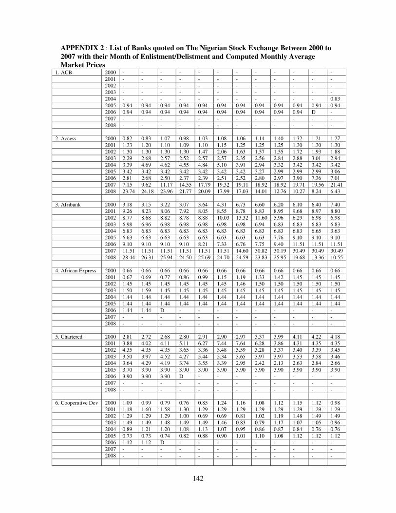
142
APPENDIX 2 : List of Banks quoted on The Nigerian Stock Exchange Between 2000 to 2007 with their Month of Enlistment/Delistment and Computed Monthly Average Market Prices
1. ACB 2000 - - - - - - - - - - - - 2001 - - - - - - - - - - - - 2002 - - - - - - - - - - - - 2003 - - - - - - - - - - - - 2004 - - - - - - - - - - - 0.83 2005 0.94 0.94 0.94 0.94 0.94 0.94 0.94 0.94 0.94 0.94 0.94 0.94 2006 0.94 0.94 0.94 0.94 0.94 0.94 0.94 0.94 0.94 0.94 D - 2007 - - - - - - - - - - - - 2008 - - - - - - - - - - - - 2. Access 2000 0.82 0.83 1.07 0.98 1.03 1.08 1.06 1.14 1.40 1.32 1.21 1.27 2001 1.33 1.20 1.10 1.09 1.10 1.15 1.25 1.25 1.25 1.30 1.30 1.30 2002 1.30 1.30 1.30 1.30 1.47 2.06 1.63 1.57 1.55 1.72 1.93 1.88 2003 2.29 2.68 2.57 2.52 2.57 2.57 2.35 2.56 2.84 2.88 3.01 2.94 2004 3.39 4.69 4.62 4.55 4.84 5.10 3.91 2.94 3.32 3.42 3.42 3.42 2005 3.42 3.42 3.42 3.42 3.42 3.42 3.42 3.27 2.99 2.99 2.99 3.06 2006 2.81 2.68 2.50 2.37 2.39 2.51 2.52 2.80 2.97 3.90 7.36 7.01 2007 7.15 9.62 11.17 14.55 17.79 19.32 19.11 18.92 18.92 19.71 19.56 21.41 2008 23.74 24.18 23.96 21.77 20.09 17.99 17.03 14.01 12.76 10.27 8.24 6.43 3. Afribank 2000 3.18 3.15 3.22 3.07 3.64 4.31 6.73 6.60 6.20 6.10 6.40 7.40 2001 9.26 8.23 8.06 7.92 8.05 8.55 8.78 8.83 8.95 9.68 8.97 8.80 2002 8.77 8.68 8.82 8.78 8.88 10.03 13.32 11.60 5.96 6.29 6.98 6.98 2003 6.98 6.96 6.98 6.98 6.98 6.98 6.98 6.94 6.83 6.83 6.83 6.83 2004 6.83 6.83 6.83 6.83 6.83 6.83 6.83 6.83 6.83 6.83 6.65 3.63 2005 6.63 6.63 6.63 6.63 6.63 6.63 6.63 6.63 7.76 9.10 9.10 9.10 2006 9.10 9.10 9.10 9.10 8.21 7.33 6.76 7.75 9.40 11.51 11.51 11.51 2007 11.51 11.51 11.51 11.51 11.51 11.51 14.60 30.82 30.19 30.49 30.49 30.49 2008 28.44 26.31 25.94 24.50 25.69 24.70 24.59 23.83 25.95 19.68 13.36 10.55 4. African Express 2000 0.66 0.66 0.66 0.66 0.66 0.66 0.66 0.66 0.66 0.66 0.66 0.66 2001 0.67 0.69 0.77 0.86 0.99 1.15 1.19 1.33 1.42 1.45 1.45 1.45 2002 1.45 1.45 1.45 1.45 1.45 1.45 1.46 1.50 1.50 1.50 1.50 1.50 2003 1.50 1.59 1.45 1.45 1.45 1.45 1.45 1.45 1.45 1.45 1.45 1.45 2004 1.44 1.44 1.44 1.44 1.44 1.44 1.44 1.44 1.44 1.44 1.44 1.44 2005 1.44 1.44 1.44 1.44 1.44 1.44 1.44 1.44 1.44 1.44 1.44 1.44 2006 1.44 1.44 D - - - - - - - - - 2007 - - - - - - - - - - - - 2008 - - - - - - - - - - - - 5. Chartered 2000 2.81 2.72 2.68 2.80 2.91 2.90 2.97 3.37 3.99 4.11 4.22 4.18 2001 3.88 4.02 4.11 5.11 6.27 7.44 7.64 6.28 3.86 4.31 4.35 4.35 2002 4.35 4.35 4.35 3.65 3.36 3.48 3.59 3.28 3.37 3.40 3.39 3.45 2003 3.50 3.97 4.52 4.27 5.44 5.34 3.65 3.97 3.97 3.53 3.58 3.46 2004 3.64 4.29 4.19 3.74 3.55 3.39 2.95 2.42 2.13 2.63 2.84 2.66 2005 3.70 3.90 3.90 3.90 3.90 3.90 3.90 3.90 3.90 3.90 3.90 3.90 2006 3.90 3.90 3.90 D - - - - - - - - 2007 - - - - - - - - - - - - 2008 - - - - - - - - - - - - 6. Cooperative Dev 2000 1.09 0.99 0.79 0.76 0.85 1.24 1.16 1.08 1.12 1.15 1.12 0.98 2001 1.18 1.60 1.58 1.30 1.29 1.29 1.29 1.29 1.29 1.29 1.29 1.29 2002 1.29 1.29 1.29 1.00 0.69 0.69 0.81 1.02 1.19 1.48 1.49 1.49 2003 1.49 1.49 1.48 1.49 1.49 1.46 0.83 0.79 1.17 1.07 1.05 0.96 2004 0.89 1.21 1.20 1.08 1.13 1.07 0.95 0.86 0.87 0.84 0.76 0.76 2005 0.73 0.73 0.74 0.82 0.88 0.90 1.01 1.10 1.08 1.12 1.12 1.12 2006 1.12 1.12 D - - - - - - - - - 2007 - - - - - - - - - - - - 2008 - - - - - - - - - - - -
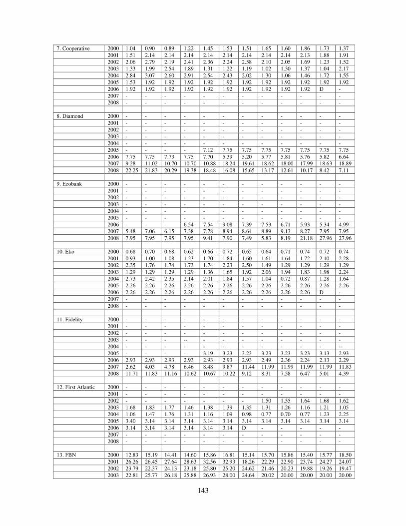
143
7. Cooperative 2000 1.04 0.90 0.89 1.22 1.45 1.53 1.51 1.65 1.60 1.86 1.73 1.37 2001 1.51 2.14 2.14 2.14 2.14 2.14 2.14 2.14 2.14 2.13 1.88 1.91 2002 2.06 2.79 2.19 2.41 2.36 2.24 2.58 2.10 2.05 1.69 1.23 1.52 2003 1.33 1.99 2.54 1.89 1.31 1.22 1.19 1.02 1.30 1.37 1.04 2.17 2004 2.84 3.07 2.60 2.91 2.54 2.43 2.02 1.30 1.06 1.46 1.72 1.55 2005 1.53 1.92 1.92 1.92 1.92 1.92 1.92 1.92 1.92 1.92 1.92 1.92 2006 1.92 1.92 1.92 1.92 1.92 1.92 1.92 1.92 1.92 1.92 D - 2007 - - - - - - - - - - - - 2008 - - - - - - - - - - - - 8. Diamond 2000 - - - - - - - - - - - - 2001 - - - - - - - - - - - - 2002 - - - - - - - - - - - - 2003 - - - - - - - - - - - - 2004 - - - - - - - - - - - - 2005 - - - - 7.12 7.75 7.75 7.75 7.75 7.75 7.75 7.75 2006 7.75 7.75 7.73 7.75 7.70 5.39 5.20 5.77 5.81 5.76 5.82 6.64 2007 9.28 11.02 10.70 10.70 10.88 18.24 19.61 18.62 18.00 17.99 18.63 18.89 2008 22.25 21.83 20.29 19.38 18.48 16.08 15.65 13.17 12.61 10.17 8.42 7.11 9. Ecobank 2000 - - - - - - - - - - - - 2001 - - - - - - - - - - - - 2002 - - - - - - - - - - - - 2003 - - - - - - - - - - - - 2004 - - - - - - - - - - - - 2005 - - - - - - - - - - - - 2006 - - - 6.54 7.54 9.08 7.39 7.53 6.71 5.93 5.34 4.99 2007 5.48 7.06 6.15 7.38 7.78 8.94 8.64 8.89 9.13 8.27 7.95 7.95 2008 7.95 7.95 7.95 7.95 9.41 7.90 7.49 5.83 8.19 21.18 27.96 27.96 10. Eko 2000 0.68 0.70 0.68 0.62 0.66 0.72 0.65 0.64 0.71 0.74 0.72 0.74 2001 0.93 1.00 1.08 1.23 1.70 1.84 1.60 1.61 1.64 1.72 2.10 2.28 2002 2.35 1.76 1.74 1.73 1.74 2.23 2.50 1.49 1.29 1.29 1.29 1.29 2003 1.29 1.29 1.29 1.29 1.36 1.65 1.92 2.06 1.94 1.83 1.98 2.24 2004 2.73 2.42 2.35 2.14 2.01 1.84 1.57 1.04 0.72 0.87 1.28 1.64 2005 2.26 2.26 2.26 2.26 2.26 2.26 2.26 2.26 2.26 2.26 2.26 2.26 2006 2.26 2.26 2.26 2.26 2.26 2.26 2.26 2.26 2.26 2.26 D - 2007 - - - - - - - - - - - - 2008 - - - - - - - - - - - - 11. Fidelity 2000 - - - - - - - - - - - - 2001 - - - - - - - - - - - - 2002 - - - - - - - - - - - - 2003 - - - -- - - - - - - - - 2004 - - - - - - - - - - - -- 2005 - - - - 3.19 3.23 3.23 3.23 3.23 3.23 3.13 2.93 2006 2.93 2.93 2.93 2.93 2.93 2.93 2.93 2.49 2.36 2.24 2.13 2.29 2007 2.62 4.03 4.78 6.46 8.48 9.87 11.44 11.99 11.99 11.99 11.99 11.83 2008 11.71 11.83 11.16 10.62 10.67 10.22 9.12 8.31 7.58 6.47 5.01 4.39 12. First Atlantic 2000 - - - - - - - - - - - - 2001 - - - - - - - - - - - - 2002 - - - - - - - 1.50 1.55 1.64 1.68 1.62 2003 1.68 1.83 1.77 1.46 1.38 1.39 1.35 1.31 1.26 1.16 1.21 1.05 2004 1.06 1.47 1.76 1.31 1.16 1.09 0.98 0.77 0.70 0.77 1.23 2.25 2005 3.40 3.14 3.14 3.14 3.14 3.14 3.14 3.14 3.14 3.14 3.14 3.14 2006 3.14 3.14 3.14 3.14 3.14 3.14 D - - - - - 2007 - - - - - - - - - - - - 2008 - - - - - - - - - - - - 13. FBN 2000 12.83 15.19 14.41 14.60 15.86 16.81 15.14 15.70 15.86 15.40 15.77 18.50 2001 26.26 26.45 27.64 28.63 32.56 32.93 18.26 22.29 22.90 23.74 24.27 24.07 2002 23.79 22.37 24.13 23.18 25.80 25.20 24.62 21.46 20.23 19.88 19.26 19.47 2003 22.81 25.77 26.18 25.88 26.93 28.00 24.64 20.02 20.00 20.00 20.00 20.00
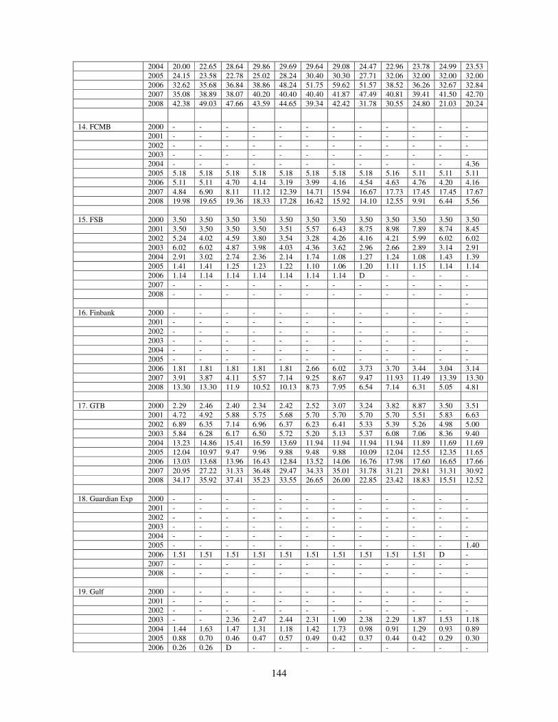
144
2004 20.00 22.65 28.64 29.86 29.69 29.64 29.08 24.47 22.96 23.78 24.99 23.53 2005 24.15 23.58 22.78 25.02 28.24 30.40 30.30 27.71 32.06 32.00 32.00 32.00 2006 32.62 35.68 36.84 38.86 48.24 51.75 59.62 51.57 38.52 36.26 32.67 32.84 2007 35.08 38.89 38.07 40.20 40.40 40.40 41.87 47.49 40.81 39.41 41.50 42.70 2008 42.38 49.03 47.66 43.59 44.65 39.34 42.42 31.78 30.55 24.80 21.03 20.24
14. FCMB 2000 - - - - - - - - - - - - 2001 - - - - - - - - - - - - 2002 - - - - - - - - - - - - 2003 - - - - - - - - - - - - 2004 - - - - - - - - - - - 4.36 2005 5.18 5.18 5.18 5.18 5.18 5.18 5.18 5.18 5.16 5.11 5.11 5.11 2006 5.11 5.11 4.70 4.14 3.19 3.99 4.16 4.54 4.63 4.76 4.20 4.16 2007 4.84 6.90 8.11 11.12 12.39 14.71 15.94 16.67 17.73 17.45 17.45 17.67 2008 19.98 19.65 19.36 18.33 17.28 16.42 15.92 14.10 12.55 9.91 6.44 5.56 15. FSB 2000 3.50 3.50 3.50 3.50 3.50 3.50 3.50 3.50 3.50 3.50 3.50 3.50 2001 3.50 3.50 3.50 3.50 3.51 5.57 6.43 8.75 8.98 7.89 8.74 8.45 2002 5.24 4.02 4.59 3.80 3.54 3.28 4.26 4.16 4.21 5.99 6.02 6.02 2003 6.02 6.02 4.87 3.98 4.03 4.36 3.62 2.96 2.66 2.89 3.14 2.91 2004 2.91 3.02 2.74 2.36 2.14 1.74 1.08 1.27 1.24 1.08 1.43 1.39 2005 1.41 1.41 1.25 1.23 1.22 1.10 1.06 1.20 1.11 1.15 1.14 1.14 2006 1.14 1.14 1.14 1.14 1.14 1.14 1.14 D - - - - 2007 - - - - - - - - - - - - 2008 - - - - - - - - - - - - - 16. Finbank 2000 - - - - - - - - - - - - 2001 - - - - - - - - - - - 2002 - - - - - - - - - - - - 2003 - - - - - - - - - - - 2004 - - - - - - - - - - - - 2005 - - - - - - - - - - - - 2006 1.81 1.81 1.81 1.81 1.81 2.66 6.02 3.73 3.70 3.44 3.04 3.14 2007 3.91 3.87 4.11 5.57 7.14 9.25 8.67 9.47 11.93 11.49 13.39 13.30 2008 13.30 13.30 11.9 10.52 10.13 8.73 7.95 6.54 7.14 6.31 5.05 4.81 17. GTB 2000 2.29 2.46 2.40 2.34 2.42 2.52 3.07 3.24 3.82 8.87 3.50 3.51 2001 4.72 4.92 5.88 5.75 5.68 5.70 5.70 5.70 5.70 5.51 5.83 6.63 2002 6.89 6.35 7.14 6.96 6.37 6.23 6.41 5.33 5.39 5.26 4.98 5.00 2003 5.84 6.28 6.17 6.50 5.72 5.20 5.13 5.37 6.08 7.06 8.36 9.40 2004 13.23 14.86 15.41 16.59 13.69 11.94 11.94 11.94 11.94 11.89 11.69 11.69 2005 12.04 10.97 9.47 9.96 9.88 9.48 9.88 10.09 12.04 12.55 12.35 11.65 2006 13.03 13.68 13.96 16.43 12.84 13.52 14.06 16.76 17.98 17.60 16.65 17.66 2007 20.95 27.22 31.33 36.48 29.47 34.33 35.01 31.78 31.21 29.81 31.31 30.92 2008 34.17 35.92 37.41 35.23 33.55 26.65 26.00 22.85 23.42 18.83 15.51 12.52 18. Guardian Exp 2000 - - - - - - - - - - - - 2001 - - - - - - - - - - - - 2002 - - - - - - - - - - - - 2003 - - - - - - - - - - - - 2004 - - - - - - - - - - - - 2005 - - - - - - - - - - - 1.40 2006 1.51 1.51 1.51 1.51 1.51 1.51 1.51 1.51 1.51 1.51 D - 2007 - - - - - - - - - - - - 2008 - - - - - - - - - - - - 19. Gulf 2000 - - - - - - - - - - - - 2001 - - - - - - - - - - - - 2002 - - - - - - - - - - - - 2003 - - 2.36 2.47 2.44 2.31 1.90 2.38 2.29 1.87 1.53 1.18 2004 1.44 1.63 1.47 1.31 1.18 1.42 1.73 0.98 0.91 1.29 0.93 0.89 2005 0.88 0.70 0.46 0.47 0.57 0.49 0.42 0.37 0.44 0.42 0.29 0.30 2006 0.26 0.26 D - - - - - - - - -

145
2007 - - - - - - - - - - - - 2008 - - - - - - - - - - - - 20. Hallmark 2000 1.50 1.50 1.60 1.81 1.79 1.75 1.97 2.07 2.15 2.14 2.20 2.09 2001 2.34 3.72 1.27 4.33 4.46 5.03 4.79 4.28 4.16 3.78 3.95 3.82 2002 3.25 3.55 3.40 3.07 2.99 2.99 3.03 2.86 2.91 2.91 2.86 2.83 2003 2.83 2.83 2.84 2.46 2.01 2.01 2.01 2.01 1.81 1.50 2.00 2.10 2004 2.17 1.99 2.06 1.96 2.04 1.89 1.82 2.12 2.13 2.25 2.08 1.61 2005 2.05 1.86 1.75 1.84 1.84 1.59 1.36 1.82 2.04 2.03 1.81 1.81 2006 1.81 1.81 D - - - - - - - - - 2007 - - - - - - - - - - - - 2008 - - - - - - - - - - - - 21. IBTC 2000 - - - - - - - - - - - - 2001 - - - - - - - - - - - - 2002 - - - - - - - - - - - - 2003 - - - - - - - - - - - - 2004 - - - - - - - - - - - - 2005 - - - - - 4.64 4.80 4.77 4.57 4.57 4.57 4.57 2006 4.57 4.57 4.57 D - - - - - - - - 2007 - - - - - - - - - - - - 2008 - - - - - - - - - - - - 22. IBTC-C 2000 - - - - - - - - - - - - 2001 - - - - - - - - - - - - 2002 - - - - - - - - - - - - 2003 - - - - - - - - - - - - 2004 - - - - - - - - - - - - 2005 - - - - 4.64 4.80 4.77 4.57 4.57 4.57 4.57 4.57 2006 4.57 4.57 4.57 5.11 5.03 4.94 4.89 5.22 5.74 6.89 6.27 6.90 2007 7.83 10.79 10.92 11.00 11.00 11.00 10.88 10.70 11.00 16.76 17.92 18.92 2008 21.79 22.47 21.49 20.28 38.80 10.06 31.19 27.45 27.20 21.98 14.16 10.64 23. ICB 2000 - - - - - - - - - - - - 2001 - - - - - - - - - - - - 2002 - - - - - - - - - - - - 2003 - 5.60 6.00 4.97 5.35 5.24 4.73 3.86 3.87 4.22 4.25 4.10 2004 4.32 5.63 5.84 5.85 5.68 6.77 6.45 5.66 5.22 7.06 7.81 7.81 2005 7.81 7.81 7.81 7.81 7.81 5.99 6.01 6.59 8.22 9.41 10.17 9.27 2006 8.78 10.02 10.05 9.98 10.67 10.57 11.62 15.60 16.13 16.13 16.02 13.98 2007 16.11 19.73 22.13 25.72 25.70 27.24 26.25 24.75 25.00 26.56 29.50 35.90 2008 10.46 42.08 44.65 45.49 32.18 24.21 22.87 20.40 21.06 17.65 13.09 11.16 24. IMB 2000 0.67 0.78 0.71 0.76 0.81 0.81 0.81 0.81 0.81 0.81 0.81 0.81 2001 0.81 0.81 0.81 0.81 0.81 1.33 1.80 1.44 1.46 1.35 1.20 1.05 2002 1.03 1.01 0.97 0.97 0.78 0.63 0.58 0.64 0.86 0.64 0.58 0.53 2003 0.52 0.73 0.67 0.57 0.56 0.52 0.60 0.58 0.53 0.52 0.49 0.63 2004 0.66 0.66 0.66 0.66 0.78 1.09 0.85 0.64 0.57 0.59 0.63 0.59 2005 0.67 0.59 0.54 0.60 0.58 0.56 0.52 0.52 0.82 0.84 0.84 0.84 2006 0.84 0.84 0.84 0.84 0.84 0.84 D - - - - - 2007 - - - - - - - - - - - - 2008 - - - - - - - - - - - - 25. Inland 2000 2.05 2.05 2.05 2.05 2.05 2.05 2.01 1.53 1.28 1.36 1.29 1.21 2001 1.83 1.85 1.82 1.56 1.64 1.46 1.54 1.52 1.24 1.36 1.49 1.20 2002 1.11 1.02 1.08 1.48 1.16 1.45 1.45 1.31 1.16 1.04 1.19 1.82 2003 1.84 1.80 1.80 1.80 1.80 1.67 1.38 1.33 1.34 1.20 1.00 0.87 2004 0.88 1.04 1.10 1.24 1.10 1.12 1.11 0.79 0.66 0.90 1.07 1.07 2005 1.13 1.34 1.57 1.81 1.81 1.81 1.81 1.81 1.81 1.81 1.81 1.81 2006 - - - - - - - - - - - - 2007 - - - - - - - - - - - - 2008 - - - - - - - - - - - - 26. Libery 2000 1.51 1.51 1.44 1.39 1.88 1.92 1.91 1.88 1.71 1.73 1.72 1.85
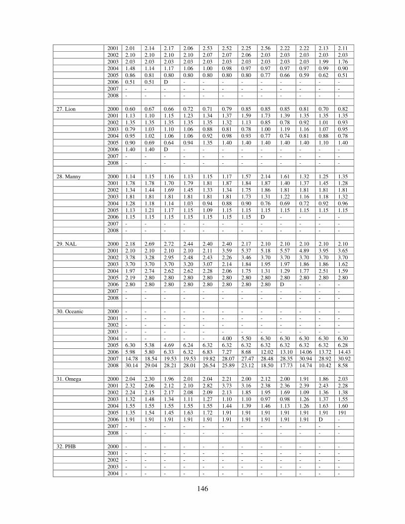
146
2001 2.01 2.14 2.17 2.06 2.53 2.52 2.25 2.56 2.22 2.22 2.13 2.11 2002 2.10 2.10 2.10 2.10 2.07 2.07 2.06 2.03 2.03 2.03 2.03 2.03 2003 2.03 2.03 2.03 2.03 2.03 2.03 2.03 2.03 2.03 2.03 1.99 1.76 2004 1.48 1.14 1.17 1.06 1.00 0.98 0.97 0.97 0.97 0.97 0.99 0.90 2005 0.86 0.81 0.80 0.80 0.80 0.80 0.80 0.77 0.66 0.59 0.62 0.51 2006 0.51 0.51 D - - - - - - - - - 2007 - - - - - - - - - - - - 2008 - - - - - - - - - - - - 27. Lion 2000 0.60 0.67 0.66 0.72 0.71 0.79 0.85 0.85 0.85 0.81 0.70 0.82 2001 1.13 1.10 1.15 1.23 1.34 1.37 1.59 1.73 1.39 1.35 1.35 1.35 2002 1.35 1.35 1.35 1.35 1.35 1.32 1.13 0.85 0.78 0.92 1.01 0.93 2003 0.79 1.03 1.10 1.06 0.88 0.81 0.78 1.00 1.19 1.16 1.07 0.95 2004 0.95 1.02 1.06 1.06 0.92 0.98 0.93 0.77 0.74 0.81 0.88 0.78 2005 0.90 0.69 0.64 0.94 1.35 1.40 1.40 1.40 1.40 1.40 1.10 1.40 2006 1.40 1.40 D - - - - - - - - - 2007 - - - - - - - - - - - - 2008 - - - - - - - - - - - - 28. Manny 2000 1.14 1.15 1.16 1.13 1.15 1.17 1.57 2.14 1.61 1.32 1.25 1.35 2001 1.78 1.78 1.70 1.79 1.81 1.87 1.84 1.87 1.40 1.37 1.45 1.28 2002 1.34 1.44 1.69 1.45 1.33 1.34 1.75 1.86 1.81 1.81 1.81 1.81 2003 1.81 1.81 1.81 1.81 1.81 1.81 1.73 1.31 1.22 1.16 1.18 1.32 2004 1.28 1.18 1.14 1.03 0.94 0.88 0.90 0.76 0.69 0.72 0.92 0.96 2005 1.13 1.21 1.17 1.15 1.09 1.15 1.15 1.15 1.15 1.15 1.15 1.15 2006 1.15 1.15 1.15 1.15 1.15 1.15 1.15 D - - - - 2007 - - - - - - - - - - - - 2008 - - - - - - - - - - - - 29. NAL 2000 2.18 2.69 2.72 2.44 2.40 2.40 2.17 2.10 2.10 2.10 2.10 2.10 2001 2.10 2.10 2.10 2.10 2.11 3.59 5.37 5.18 5.57 4.89 3.95 3.65 2002 3.78 3.28 2.95 2.48 2.43 2.26 3.46 3.70 3.70 3.70 3.70 3.70 2003 3.70 3.70 3.70 3.20 3.07 2.14 1.84 1.95 1.97 1.86 1.86 1.62 2004 1.97 2.74 2.62 2.62 2.28 2.06 1.75 1.31 1.29 1.77 2.51 1.59 2005 2.19 2.80 2.80 2.80 2.80 2.80 2.80 2.80 2.80 2.80 2.80 2.80 2006 2.80 2.80 2.80 2.80 2.80 2.80 2.80 2.80 D - - - 2007 - - - - - - - - - - - - 2008 - - - - - - - - - - - - 30. Oceanic 2000 - - - - - - - - - - - - 2001 - - - - - - - - - - - - 2002 - - - - - - - - - - - - 2003 - - - - - - - - - - - - 2004 - - - - - 4.00 5.50 6.30 6.30 6.30 6.30 6.30 2005 6.30 5.38 4.69 6.24 6.32 6.32 6.32 6.32 6.32 6.32 6.32 6.28 2006 5.98 5.80 6.33 6.32 6.83 7.27 8.68 12.02 13.10 14.06 13.72 14.43 2007 14.78 18.54 19.53 19.53 19.82 28.07 27.47 28.48 28.35 30.94 28.92 30.92 2008 30.14 29.04 28.21 28.01 26.54 25.89 23.12 18.50 17.73 14.74 10.42 8.58 31. Omega 2000 2.04 2.30 1.96 2.01 2.04 2.21 2.00 2.12 2.00 1.91 1.86 2.03 2001 2.32 2.06 2.12 2.10 2.82 3.73 3.16 2.38 2.36 2.39 2.43 2.28 2002 2.24 2.15 2.17 2.08 2.09 2.13 1.85 1.95 1.69 1.09 1.36 1.38 2003 1.32 1.48 1.34 1.11 1.27 1.10 1.10 0.97 0.98 1.26 1.37 1.55 2004 1.55 1.55 1.55 1.55 1.55 1.44 1.39 1.46 1.13 1.26 1.63 1.60 2005 1.35 1.54 1.45 1.63 1.72 1.91 1.91 1.91 1.91 1.91 1.91 191 2006 1.91 1.91 1.91 1.91 1.91 1.91 1.91 1.91 1.91 1.91 D - 2007 - - - - - - - - - - - - 2008 - - - - - - - - - - - - 32. PHB 2000 - - - - - - - - - - - - 2001 - - - - - - - - - - - - 2002 - - - - - - - - - - - - 2003 - - - - - - - - - - - - 2004 - - - - - - - - - - - -

147
2005 - - - - - - - - - - - 2.59 2006 2.60 2.60 2.60 2.60 2.60 2.60 2.43 2.39 2.54 2.41 2.77 3.22 2007 3.24 4.96 5.43 7.04 17.10 22.59 28.39 29.45 28.78 30.98 27.54 25.51 2008 27.55 30.10 30.42 28.84 19.65 15.10 15.25 13.12 12.75 11.29 9.21 7.18 33. Prudent 2000 - - - - - - - - - - - - 2001 - - - - - - - - - - - - 2002 - - - - - - - - - - - - 2003 - - - - - - - - - - - - 2004 - - - - - - - - - - - - 2005 - - - - - - - - - - 2.31 3.02 2006 3.06 2.95 3.06 3.06 3.06 3.06 3.06 3.06 3.06 3.06 D - 2007 - - - - - - - - - - - - 2008 - - - - - - - - - - - - 34. Regent 2000 - - - - - - - - - - - - 2001 - - - - - - - - - - - - 2002 - - - - - - - - - - - - 2003 - - - - - - - - 0.68 1.17 1.15 1.03 2004 1.05 1.18 1.16 1.12 1.01 1.00 0.95 0.91 0.91 0.91 0.86 0.85 2005 0.82 0.81 0.81 0.81 0.81 0.81 0.81 0.81 0.83 0.89 0.89 0.89 2006 0.89 0.89 0.89 D - - - - - - - - 2007 - - - - - - - - - - - - 2008 - - - - - - - - - - - - 35. Savannah 2000 1.10 1.17 1.02 1.10 1.17 1.28 1.48 1.63 1.46 1.31 1.25 1.29 2001 1.55 1.51 1.47 1.28 1.30 1.26 1.22 1.27 1.25 1.35 1.18 1.02 2002 0.95 0.81 0.80 0.80 0.80 0.80 0.80 0.80 0.80 0.80 0.80 0.80 2003 0.80 0.80 0.80 0.80 0.80 0.80 0.80 0.80 0.80 0.80 0.80 0.80 2004 0.80 0.80 0.80 0.80 0.80 0.80 0.80 0.80 0.80 0.80 0.80 0.80 2005 0.80 0.80 0.80 0.80 0.80 0.80 0.80 0.80 0.80 0.80 0.80 0.80 2006 0.80 0.80 D - - - - - - - - - 2007 - - - - - - - - - - - - 2008 - - - - - - - - - - - - 36. Skye 2000 - - - - - - - - - - - - 2001 - - - - - - - - - - - - 2002 - - - - - - - - - - - - 2003 - - - - - - - - - - - - 2004 - - - - - - - - - - - - 2005 - - - - - - - - - - - - 2006 - - - - - - - - - - 5.80 4.70 2007 3.91 5.87 5.87 7.08 8.31 12.04 12.69 12.53 13.60 14.95 16.05 5.73 2008 16.97 16.84 17.09 17.84 16.25 17.20 14.87 12.54 12.93 10.72 9.77 8.83 37. Spring 2000 - - - - - - - - - - - - 2001 - - - - - - - - - - - - 2002 - - - - - - - - - - - - 2003 - - - - - - - - - - - - 2004 - - - - - - - - - - - - 2005 - - - - - - - - - - - - 2006 - - - - - - - - - - - - 2007 5.36 5.00 5.59 5.59 5.59 5.59 5.59 5.59 5.59 5.59 5.59 5.59 2008 5.59 5.59 5.59 5.59 8.44 5.59 5.59 5.59 5.59 5.59 5.59 5.59 38. Sterling 2000 - - - - - - - - - - - - 2001 - - - - - - - - - - - - 2002 - - - - - - - - - - - - 2003 - - - - - - - - - - - - 2004 - - - - - - - - - - - - 2005 - - - - - - -- - - - - - 2006 - - - - - - - - 2.80 6.36 5.32 4.34 2007 3.45 4.46 4.32 5.49 6.57 8.89 8.15 7.88 7.75 7.33 7.27 7.28 2008 7.28 7.28 7.28 7.28 7.49 6.70 6.68 6.65 5.90 4.94 3.73 2.56
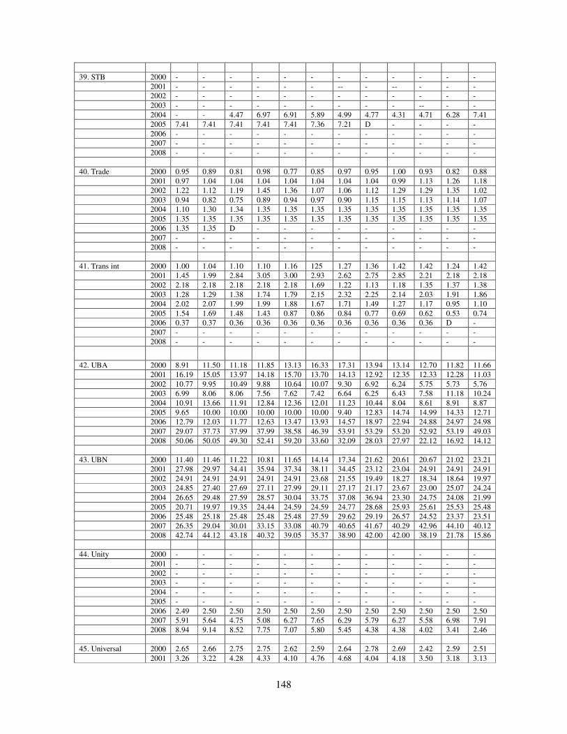
148
39. STB 2000 - - - - - - - - - - - - 2001 - - - - - - -- - -- - - - 2002 - - - - - - - - - - - - 2003 - - - - - - - - - -- - - 2004 - - 4.47 6.97 6.91 5.89 4.99 4.77 4.31 4.71 6.28 7.41 2005 7.41 7.41 7.41 7.41 7.41 7.36 7.21 D - - - - 2006 - - - - - - - - - - - - 2007 - - - - - - - - - - - - 2008 - - - - - - - - - - - - 40. Trade 2000 0.95 0.89 0.81 0.98 0.77 0.85 0.97 0.95 1.00 0.93 0.82 0.88 2001 0.97 1.04 1.04 1.04 1.04 1.04 1.04 1.04 0.99 1.13 1.26 1.18 2002 1.22 1.12 1.19 1.45 1.36 1.07 1.06 1.12 1.29 1.29 1.35 1.02 2003 0.94 0.82 0.75 0.89 0.94 0.97 0.90 1.15 1.15 1.13 1.14 1.07 2004 1.10 1.30 1.34 1.35 1.35 1.35 1.35 1.35 1.35 1.35 1.35 1.35 2005 1.35 1.35 1.35 1.35 1.35 1.35 1.35 1.35 1.35 1.35 1.35 1.35 2006 1.35 1.35 D - - - - - - - - - 2007 - - - - - - - - - - - - 2008 - - - - - - - - - - - - 41. Trans int 2000 1.00 1.04 1.10 1.10 1.16 125 1.27 1.36 1.42 1.42 1.24 1.42 2001 1.45 1.99 2.84 3.05 3.00 2.93 2.62 2.75 2.85 2.21 2.18 2.18 2002 2.18 2.18 2.18 2.18 2.18 1.69 1.22 1.13 1.18 1.35 1.37 1.38 2003 1.28 1.29 1.38 1.74 1.79 2.15 2.32 2.25 2.14 2.03 1.91 1.86 2004 2.02 2.07 1.99 1.99 1.88 1.67 1.71 1.49 1.27 1.17 0.95 1.10 2005 1.54 1.69 1.48 1.43 0.87 0.86 0.84 0.77 0.69 0.62 0.53 0.74 2006 0.37 0.37 0.36 0.36 0.36 0.36 0.36 0.36 0.36 0.36 D - 2007 - - - - - - - - - - - - 2008 - - - - - - - - - - - -
42. UBA 2000 8.91 11.50 11.18 11.85 13.13 16.33 17.31 13.94 13.14 12.70 11.82 11.66 2001 16.19 15.05 13.97 14.18 15.70 13.70 14.13 12.92 12.35 12.33 12.28 11.03 2002 10.77 9.95 10.49 9.88 10.64 10.07 9.30 6.92 6.24 5.75 5.73 5.76 2003 6.99 8.06 8.06 7.56 7.62 7.42 6.64 6.25 6.43 7.58 11.18 10.24 2004 10.91 13.66 11.91 12.84 12.36 12.01 11.23 10.44 8.04 8.61 8.91 8.87 2005 9.65 10.00 10.00 10.00 10.00 10.00 9.40 12.83 14.74 14.99 14.33 12.71 2006 12.79 12.03 11.77 12.63 13.47 13.93 14.57 18.97 22.94 24.88 24.97 24.98 2007 29.07 37.73 37.99 37.99 38.58 46.39 53.91 53.29 53.20 52.92 53.19 49.03 2008 50.06 50.05 49.30 52.41 59.20 33.60 32.09 28.03 27.97 22.12 16.92 14.12 43. UBN 2000 11.40 11.46 11.22 10.81 11.65 14.14 17.34 21.62 20.61 20.67 21.02 23.21 2001 27.98 29.97 34.41 35.94 37.34 38.11 34.45 23.12 23.04 24.91 24.91 24.91 2002 24.91 24.91 24.91 24.91 24.91 23.68 21.55 19.49 18.27 18.34 18.64 19.97 2003 24.85 27.40 27.69 27.11 27.99 29.11 27.17 21.17 23.67 23.00 25.07 24.24 2004 26.65 29.48 27.59 28.57 30.04 33.75 37.08 36.94 23.30 24.75 24.08 21.99 2005 20.71 19.97 19.35 24.44 24.59 24.59 24.77 28.68 25.93 25.61 25.53 25.48 2006 25.48 25.18 25.48 25.48 25.48 27.59 29.62 29.19 26.57 24.52 23.37 23.51 2007 26.35 29.04 30.01 33.15 33.08 40.79 40.65 41.67 40.29 42.96 44.10 40.12 2008 42.74 44.12 43.18 40.32 39.05 35.37 38.90 42.00 42.00 38.19 21.78 15.86 44. Unity 2000 - - - - - - - - - - - - 2001 - - - - - - - - - - - - 2002 - - - - - - - - - - - - 2003 - - - - - - - - - - - - 2004 - - - - - - - - - - - - 2005 - - - - - - - - - - - - 2006 2.49 2.50 2.50 2.50 2.50 2.50 2.50 2.50 2.50 2.50 2.50 2.50 2007 5.91 5.64 4.75 5.08 6.27 7.65 6.29 5.79 6.27 5.58 6.98 7.91 2008 8.94 9.14 8.52 7.75 7.07 5.80 5.45 4.38 4.38 4.02 3.41 2.46 45. Universal 2000 2.65 2.66 2.75 2.75 2.62 2.59 2.64 2.78 2.69 2.42 2.59 2.51 2001 3.26 3.22 4.28 4.33 4.10 4.76 4.68 4.04 4.18 3.50 3.18 3.13
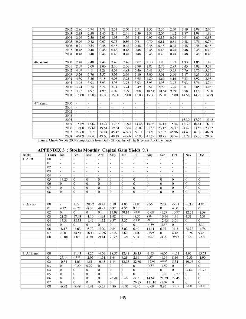
149
2002 2.96 2.94 2.78 2.51 2.60 2.51 2.55 2.35 2.30 2.19 2.09 2.00 2003 2.13 2.50 2.45 2.44 2.41 2.39 2.33 2.06 1.92 1.87 1.98 1.89 2004 2.99 2.30 2.05 1.93 1.79 1.41 0.97 0.87 0.74 0.91 1.00 0.83 2005 0.99 0.82 0.67 0.73 0.89 0.81 0.70 0.81 0.81 0.88 0.76 0.76 2006 0.71 0.55 0.48 0.48 0.48 0.48 0.48 0.48 0.48 0.48 0.48 0.48 2007 0.48 0.48 0.48 0.48 0.48 0.48 0.48 0.48 0.48 0.48 0.48 0.48 2008 0.48 0.48 0.48 0.48 0.48 0.48 0.48 0.48 0.48 0.48 0.48 0.48 46. Wema 2000 2.48 2.48 2.48 2.48 2.46 2.07 2.10 1.99 1.97 1.93 1.85 1.89 2001 2.07 2.00 2.00 2.10 2.56 2.79 2.83 2.73 2.93 3.45 3.82 3.57 2002 4.09 4.11 4.28 4.64 4.83 5.46 5.41 5.16 5.75 5.76 5.76 5.76 2003 5.76 5.76 5.57 3.07 2.99 3.10 3.00 3.01 3.00 3.17 4.23 3.89 2004 4.50 5.36 6.18 6.03 5.93 5.65 4.80 4.64 4.16 3.43 3.92 3.93 2005 3.93 3.93 3.93 3.93 3.93 3.93 3.93 3.93 3.93 3.93 3.76 3.74 2006 3.74 3.74 3.74 3.74 3.74 3.49 2.51 2.92 3.26 3.01 3.05 3.06 2007 3.92 4.97 4.99 6.07 7.29 9.08 10.54 10.54 9.89 9.58 13.80 15.00 2008 15.00 15.00 15.00 15.00 15.00 15.00 15.00 15.00 15.00 14.58 14.29 14.29 47. Zenith 2000 - - - - - - - - - - - - 2001 - - - - - - - - - - - - 2002 - - - - - - - - - - - - 2003 - - - - - - - - - - - - 2004 - - - - - - - - - 13.30 17.70 15.42 2005 15.69 13.62 13.27 13.67 13.92 14.46 15.06 14.15 15.54 16.39 16.61 16.01 2006 19.08 19.64 19.64 19.64 19.64 20.02 21.56 23.12 24.37 24.47 23.58 23.82 2007 27.68 32.79 36.14 45.42 49.63 60.11 63.50 57.02 45.96 44.43 46.09 46.09 2008 46.09 49.43 49.60 48.18 48.66 43.93 41.59 39.75 38.54 32.28 25.30 20.56
Source: Chuke Nwude 2009 computation from Daily Official list of The Nigerian Stock Exchange APPENDIX 3 : Stocks Monthly Capital Gain Yields(%)
Banks Years Jan Feb Mar Apr May Jun Jul Aug Sep Oct Nov Dec 1. ACB 00 - - - - - - - - - - - - 01 - - - - - - - - - - - - 02 - - - - - - - - - - - - 03 - - - - - - - - - - - - 04 - - - - - - - - - - - - 05 13.25 0 0 0 0 0 0 0 0 0 0 0 06 0 0 0 0 0 0 0 0 0 0 0 0 07 0 0 0 0 0 0 0 0 0 0 0 0 08 0 0 0 0 0 0 0 0 0 0 0 0 2. Access 00 - 1.22 28.92 -8.41 5.10 4.85 -1.85 7.55 22.81 -5.71 -8.33 4.96 01 4.72 -9.77 -8.33 -0.91 0.92 4.55 8.70 0 0 4.00 0 0 02 0 0 0 0 13.08 40.14 -20.87 -3.68 -1.27 10.97 12.21 -2.59 03 21.81 17.03 -4.10 -1.95 1.98 0 -8.56 8.94 10.94 1.41 4.51 -2.33 04 15.31 38.35 -1.49 -1.52 6.37 5.37 -23.33 -24.81 12.93 3.01 0 0 05 0 0 0 0 0 0 0 -4.39 -8.56 0 0 2.34 06 -8.17 -4.63 -6.72 -5.20 0.84 5.02 0.40 11.11 6.07 31.31 88.72 -4.76 07 2.00 34.55 16.11 30.26 22.27 8.60 -1.09 -0.99 0 4.18 -0.76 9.46 08 10.88 1.85 -0.91 -9.14 -7.72 -10.45 5.34 -17.73 -8.92 -19.51 -19.77 -21.97 3. Afribank 00 - 11.43 -8.26 -4.66 18.57 18.41 56.15 -1.93 -6.06 -1.61 4.92 15.63 01 25.14 -11.12 -2.07 -1.74 1.64 6.21 2.69 0.57 -1.36 8.16 -7.33 -1.90 02 -0.34 -1.03 1.61 -0.45 1.14 12.95 32.80 -12.91 -48.62 5.54 10.97 0 03 0 -0.29 0.29 0 0 0 0 -0.57 -1.59 0 0 0 04 0 0 0 0 0 0 0 0 0 0 -2.64 -0.30 05 0 0 0 0 0 0 0 0 1.96 17.27 0 0 06 0 0 0 0 -9.78 -10.72 -7.78 14.64 21.29 22.45 0 0 07 0 0 0 0 0 0 26.85 111.10 -1.07 0 0 0 08 -6.72 -7.49 -1.41 -5.55 4.86 -3.85 -0.45 -3.09 8.90 -24.16 -32.11 -21.03
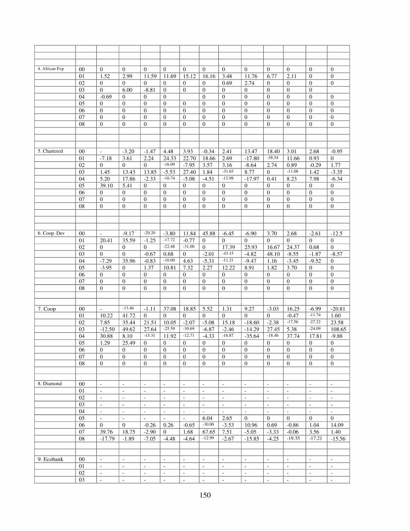
150
4. African Exp 00 0 0 0 0 0 0 0 0 0 0 0 0 01 1.52 2.99 11.59 11.69 15.12 16.16 3.48 11.76 6.77 2.11 0 0 02 0 0 0 0 0 0 0.69 2.74 0 0 0 0 03 0 6.00 -8.81 0 0 0 0 0 0 0 0 04 -0.69 0 0 0 0 0 0 0 0 0 0 05 0 0 0 0 0 0 0 0 0 0 0 0 06 0 0 0 0 0 0 0 0 0 0 0 0 07 0 0 0 0 0 0 0 0 0 0 0 0 08 0 0 0 0 0 0 0 0 0 0 0 0 5. Chartered 00 - -3.20 -1.47 4.48 3.93 -0.34 2.41 13.47 18.40 3.01 2.68 -0.95 01 -7.18 3.61 2.24 24.33 22.70 18.66 2.69 -17.80 -38.54 11.66 0.93 0 02 0 0 0 -16.09 -7.95 3.57 3.16 -8.64 2.74 0.89 -0.29 1.77 03 1.45 13.43 13.85 -5.53 27.40 1.84 -31.65 8.77 0 -11.08 1.42 -3.35 04 5.20 17.86 -2.33 -10.74 -5.08 -4.51 -12.98 -17.97 0.41 8.23 7.98 -6.34 05 39.10 5.41 0 0 0 0 0 0 0 0 0 0 06 0 0 0 0 0 0 0 0 0 0 0 0 07 0 0 0 0 0 0 0 0 0 0 0 0 08 0 0 0 0 0 0 0 0 0 0 0 0 6. Coop. Dev 00 - -9.17 -20.20 -3.80 11.84 45.88 -6.45 -6.90 3.70 2.68 -2.61 -12.5 01 20.41 35.59 -1.25 -17.72 -0.77 0 0 0 0 0 0 0 02 0 0 0 -22.48 -31.00 0 17.39 25.93 16.67 24.37 0.68 0 03 0 0 -0.67 0.68 0 -2.01 -43.15 -4.82 48.10 -8.55 -1.87 -8.57 04 -7.29 35.96 -0.83 -10.00 4.63 -5.31 -11.21 -9.47 1.16 -3.45 -9.52 0 05 -3.95 0 1.37 10.81 7.32 2.27 12.22 8.91 1.82 3.70 0 0 06 0 0 0 0 0 0 0 0 0 0 0 0 07 0 0 0 0 0 0 0 0 0 0 0 0 08 0 0 0 0 0 0 0 0 0 0 0 0 7. Coop 00 - -13.46 -1.11 37.08 18.85 5.52 1.31 9.27 -3.03 16.25 -6.99 -20.81 01 10.22 41.72 0 0 0 0 0 0 0 -0.47 -11.74 1.60 02 7.85 35.44 21.51 10.05 -2.07 -5.08 15.18 -18.60 -2.38 -17.56 -27.22 23.58 03 -12.50 49.62 27.64 -25.59 -30.69 -6.87 -2.46 -14.29 27.45 5.38 -24.09 108.65 04 30.88 8.10 -15.31 11.92 -12.71 -4.33 -16.87 -35.64 -18.46 37.74 17.81 -9.88 05 1.29 25.49 0 0 0 0 0 0 0 0 0 0 06 0 0 0 0 0 0 0 0 0 0 0 0 07 0 0 0 0 0 0 0 0 0 0 0 0 08 0 0 0 0 0 0 0 0 0 0 0 0 8. Diamond 00 - - - - - - - - - - - - 01 - - - - - - - - - - - - 02 - - - - - - - - - - - - 03 - - - - - - - - - - - - 04 - - - - - - - - - - - - 05 - - - - - 6.04 2.65 0 0 0 0 0 06 0 0 -0.26 0.26 -0.65 -30.00 -3.53 10.96 0.69 -0.86 1.04 14.09 07 39.76 18.75 -2.90 0 1.68 67.65 7.51 -5.05 -3.33 -0.06 3.56 1.40 08 -17.79 -1.89 -7.05 -4.48 -4.64 -12.99 -2.67 -15.85 -4.25 -19.35 -17.21 -15.56 9. Ecobank 00 - - - - - - - - - - - - 01 - - - - - - - - - - - - 02 - - - - - - - - - - - - 03 - - - - - - - - - - - -
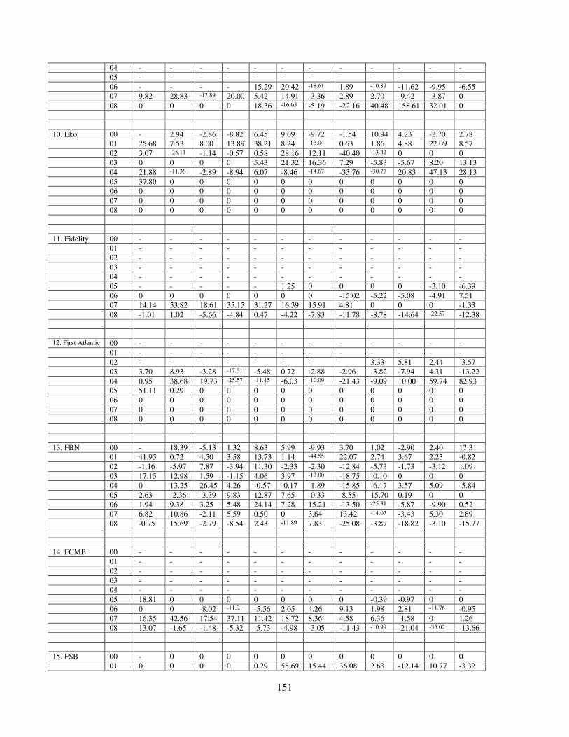
151
04 - - - - - - - - - - - - 05 - - - - - - - - - - - - 06 - - - - 15.29 20.42 -18.61 1.89 -10.89 -11.62 -9.95 -6.55 07 9.82 28.83 -12.89 20.00 5.42 14.91 -3.36 2.89 2.70 -9.42 -3.87 0 08 0 0 0 0 18.36 -16.05 -5.19 -22.16 40.48 158.61 32.01 0 10. Eko 00 - 2.94 -2.86 -8.82 6.45 9.09 -9.72 -1.54 10.94 4.23 -2.70 2.78 01 25.68 7.53 8.00 13.89 38.21 8.24 -13.04 0.63 1.86 4.88 22.09 8.57 02 3.07 -25.11 -1.14 -0.57 0.58 28.16 12.11 -40.40 -13.42 0 0 0 03 0 0 0 0 5.43 21.32 16.36 7.29 -5.83 -5.67 8.20 13.13 04 21.88 -11.36 -2.89 -8.94 6.07 -8.46 -14.67 -33.76 -30.77 20.83 47.13 28.13 05 37.80 0 0 0 0 0 0 0 0 0 0 0 06 0 0 0 0 0 0 0 0 0 0 0 0 07 0 0 0 0 0 0 0 0 0 0 0 0 08 0 0 0 0 0 0 0 0 0 0 0 0 11. Fidelity 00 - - - - - - - - - - - - 01 - - - - - - - - - - - - 02 - - - - - - - - - - - - 03 - - - - - - - - - - - - 04 - - - - - - - - - - - - 05 - - - - - 1.25 0 0 0 0 -3.10 -6.39 06 0 0 0 0 0 0 0 -15.02 -5.22 -5.08 -4.91 7.51 07 14.14 53.82 18.61 35.15 31.27 16.39 15.91 4.81 0 0 0 -1.33 08 -1.01 1.02 -5.66 -4.84 0.47 -4.22 -7.83 -11.78 -8.78 -14.64 -22.57 -12.38 12. First Atlantic 00 - - - - - - - - - - - - 01 - - - - - - - - - - - - 02 - - - - - - - - 3.33 5.81 2.44 -3.57 03 3.70 8.93 -3.28 -17.51 -5.48 0.72 -2.88 -2.96 -3.82 -7.94 4.31 -13.22 04 0.95 38.68 19.73 -25.57 -11.45 -6.03 -10.09 -21.43 -9.09 10.00 59.74 82.93 05 51.11 0.29 0 0 0 0 0 0 0 0 0 0 06 0 0 0 0 0 0 0 0 0 0 0 0 07 0 0 0 0 0 0 0 0 0 0 0 0 08 0 0 0 0 0 0 0 0 0 0 0 0 13. FBN 00 - 18.39 -5.13 1.32 8.63 5.99 -9.93 3.70 1.02 -2.90 2.40 17.31 01 41.95 0.72 4.50 3.58 13.73 1.14 -44.55 22.07 2.74 3.67 2.23 -0.82 02 -1.16 -5.97 7.87 -3.94 11.30 -2.33 -2.30 -12.84 -5.73 -1.73 -3.12 1.09 03 17.15 12.98 1.59 -1.15 4.06 3.97 -12.00 -18.75 -0.10 0 0 0 04 0 13.25 26.45 4.26 -0.57 -0.17 -1.89 -15.85 -6.17 3.57 5.09 -5.84 05 2.63 -2.36 -3.39 9.83 12.87 7.65 -0.33 -8.55 15.70 0.19 0 0 06 1.94 9.38 3.25 5.48 24.14 7.28 15.21 -13.50 -25.31 -5.87 -9.90 0.52 07 6.82 10.86 -2.11 5.59 0.50 0 3.64 13.42 -14.07 -3.43 5.30 2.89 08 -0.75 15.69 -2.79 -8.54 2.43 -11.89 7.83 -25.08 -3.87 -18.82 -3.10 -15.77 14. FCMB 00 - - - - - - - - - - - - 01 - - - - - - - - - - - - 02 - - - - - - - - - - - - 03 - - - - - - - - - - - - 04 - - - - - - - - - - - - 05 18.81 0 0 0 0 0 0 0 -0.39 -0.97 0 0 06 0 0 -8.02 -11.91 -5.56 2.05 4.26 9.13 1.98 2.81 -11.76 -0.95 07 16.35 42.56 17.54 37.11 11.42 18.72 8.36 4.58 6.36 -1.58 0 1.26 08 13.07 -1.65 -1.48 -5.32 -5.73 -4.98 -3.05 -11.43 -10.99 -21.04 -35.02 -13.66 15. FSB 00 - 0 0 0 0 0 0 0 0 0 0 0 01 0 0 0 0 0.29 58.69 15.44 36.08 2.63 -12.14 10.77 -3.32
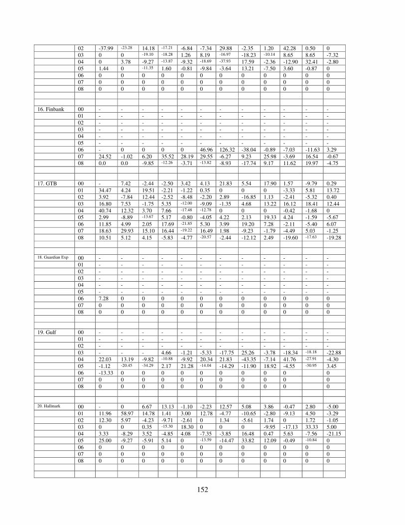
152
02 -37.99 -23.28 14.18 -17.21 -6.84 -7.34 29.88 -2.35 1.20 42.28 0.50 0 03 0 0 -19.10 -18.28 1.26 8.19 -16.97 -18.23 -10.14 8.65 8.65 -7.32 04 0 3.78 -9.27 -13.87 -9.32 -18.69 -37.93 17.59 -2.36 -12.90 32.41 -2.80 05 1.44 0 -11.35 1.60 -0.81 -9.84 -3.64 13.21 -7.50 3.60 -0.87 0 06 0 0 0 0 0 0 0 0 0 0 0 0 07 0 0 0 0 0 0 0 0 0 0 0 0 08 0 0 0 0 0 0 0 0 0 0 0 0 16. Finbank 00 - - - - - - - - - - - - 01 - - - - - - - - - - - - 02 - - - - - - - - - - - - 03 - - - - - - - - - - - - 04 - - - - - - - - - - - - 05 - - - - - - - - - - - - 06 - 0 0 0 0 46.96 126.32 -38.04 -0.89 -7.03 -11.63 3.29 07 24.52 -1.02 6.20 35.52 28.19 29.55 -6.27 9.23 25.98 -3.69 16.54 -0.67 08 0.0 0.0 -9.85 -12.26 -3.71 -13.82 -8.93 -17.74 9.17 11.62 19.97 -4.75 17. GTB 00 - 7.42 -2.44 -2.50 3.42 4.13 21.83 5.54 17.90 1.57 -9.79 0.29 01 34.47 4.24 19.51 -2.21 -1.22 0.35 0 0 0 -3.33 5.81 13.72 02 3.92 -7.84 12.44 -2.52 -8.48 -2.20 2.89 -16.85 1.13 -2.41 -5.32 0.40 03 16.80 7.53 -1.75 5.35 -12.00 -9.09 -1.35 4.68 13.22 16.12 18.41 12.44 04 40.74 12.32 3.70 7.66 -17.48 -12.78 0 0 0 -0.42 -1.68 0 05 2.99 -8.89 -13.67 5.17 -0.80 -4.05 4.22 2.13 19.33 4.24 -1.59 -5.67 06 11.85 4.99 2.05 17.69 -21.85 5.30 3.99 19.20 7.28 -2.11 -5.40 6.07 07 18.63 29.93 15.10 16.44 -19.22 16.49 1.98 -9.23 -1.79 -4.49 5.03 -1.25 08 10.51 5.12 4.15 -5.83 -4.77 -20.57 -2.44 -12.12 2.49 -19.60 -17.63 -19.28 18. Guardian Exp 00 - - - - - - - - - - - - 01 - - - - - - - - - - - - 02 - - - - - - - - - - - - 03 - - - - - - - - - - - - 04 - - - - - - - - - - - - 05 - - - - - - - - - - - - 06 7.28 0 0 0 0 0 0 0 0 0 0 0 07 0 0 0 0 0 0 0 0 0 0 0 0 08 0 0 0 0 0 0 0 0 0 0 0 0 19. Gulf 00 - - - - - - - - - - - - 01 - - - - - - - - - - - - 02 - - - - - - - - - - - - 03 - - - 4.66 -1.21 -5.33 -17.75 25.26 -3.78 -18.34 -18.18 -22.88 04 22.03 13.19 -9.82 -10.88 -9.92 20.34 21.83 -43.35 -7.14 41.76 -27.91 -4.30 05 -1.12 -20.45 -34.29 2.17 21.28 -14.04 -14.29 -11.90 18.92 -4.55 -30.95 3.45 06 -13.33 0 0 0 0 0 0 0 0 0 0 07 0 0 0 0 0 0 0 0 0 0 0 08 0 0 0 0 0 0 0 0 0 0 0 20. Hallmark 00 - 0 6.67 13.13 -1.10 -2.23 12.57 5.08 3.86 -0.47 2.80 -5.00 01 11.96 58.97 14.78 1.41 3.00 12.78 -4.77 -10.65 -2.80 -9.13 4.50 -3.29 02 12.30 5.97 -4.23 -9.71 -2.61 0 1.34 -5.61 1.74 0 1.72 -1.05 03 0 0 0.35 -15.30 18.30 0 0 0 -9.95 -17.13 33.33 5.00 04 3.33 -8.29 3.52 -4.85 4.08 -7.35 -3.85 16.48 0.47 5.63 -7.56 -21.15 05 25.00 -9.27 -5.91 5.14 0 -13.59 -14.47 33.82 12.09 -0.49 -10.84 0 06 0 0 0 0 0 0 0 0 0 0 0 0 07 0 0 0 0 0 0 0 0 0 0 0 0 08 0 0 0 0 0 0 0 0 0 0 0 0

153
21. IBTC 00 - - - - - - - - - - - - 01 - - - - - - - - - - - - 02 - - - - - - - - - - - - 03 - - - - - - - - - - - - 04 - - - - - - - - - - - - 05 - - - - - 3.45 -0.63 -4.19 0 0 0 0 06 0 0 0 11.82 1.57 -1.79 -1.01 6.75 9.96 20.03 -9.00 10.05 07 13.48 37.80 1.20 0.73 0 0 -2.00 -1.65 2.80 52.36 6.92 5.58 08 15.17 3.12 -4.36 -5.63 91.32 3.25 -22.14 11.99 -0.91 -19.19 -35.58 -24.86 22. ICB 00 - - - - - - - - - - - - 01 - - - - - - - - - - - - 02 - - - - - - - - - - - - 03 - - 7.14 -17.17 7.65 -2.06 -9.73 193.02 -72.08 9.04 0.71 -3.53 04 5.09 30.32 3.73 0.17 -2.91 -19.19 -4.73 -12.25 -7.77 35.25 10.62 0 05 0 0 0 0 0 -23.30 0.33 -9.65 24.73 -14.48 8.08 -8.85 06 -5.29 14.12 0.30 -0.70 6.91 -0.94 10.22 33.91 3.40 0 -0.68 -12.73 07 17.38 20.23 12.16 16.22 -0.08 5.99 -3.63 -5.71 1.01 6.24 11.07 21.69 08 12.70 4.00 6.11 1.88 -29.26 -24.77 -5.53 -10.80 3.24 -16.19 -25.84 -14.74 23. IMB 00 - 16.42 -5.13 2.70 6.58 0 0 0 0 0 0 0 01 0 0 0 0 0 64.20 35.34 -20.00 1.39 -7.53 -11.11 -12.5 02 -1.90 -1.94 -3.96 0 -19.59 -19.23 -7.94 10.34 34.38 -25.58 -9.38 -8.62 03 -1.89 40.38 -8.22 -14.93 -1.75 -7.14 15.38 -3.33 -8.62 -1.89 -5.77 28.57 04 4.76 0 0 0 18.18 39.74 -22.02 -21.70 -10.94 3.50 6.78 -6.35 05 13.56 -11.94 -8.47 11.11 -3.33 -3.45 -10.71 0 57.69 2.44 0 0 06 0 0 0 0 0 0 0 0 0 0 0 0 07 0 0 0 0 0 0 0 0 0 0 0 0 08 0 0 0 0 0 0 0 0 0 0 0 0 24. Inland 00 - 0 -4.64 -3.47 35.25 2.13 -0.52 -1.57 -9.04 1.17 0.58 7.56 01 8.65 6.47 1.41 -5.07 22.82 -0.40 -10.72 13.29 -13.29 0 -4.06 -0.94 02 -0.48 0 0 0 -1.43 0 -0.49 -1.46 0 0 0 0 03 0 0 0 0 0 0 0 0 0 0 -1.97 -11.56 04 -15.91 -22.98 2.64 -9.41 -5.66 -2.00 -1.02 0 0 0 2.06 -9.09 05 1.44 -5.81 -1.23 0 0 0 0 -3.75 -14.29 -10.61 5.09 -17.74 06 0 0 0 0 0 0 0 0 0 0 0 0 07 0 0 0 0 0 0 0 0 0 0 0 0 08 0 0 0 0 0 0 0 0 0 0 0 0 25. Liberty 00 - 11.67 1.49 9.09 -1.39 11.27 7.59 0 0 -4.71 -13.58 17.14 01 37.80 -2.65 4.55 6.96 8.94 2.24 16.06 8.81 -19.65 -2.88 0 0 02 0 0 0 0 0 -2.22 -14.39 -24.78 -8.24 17.95 9.78 -7.92 03 -15.05 30.38 6.80 -3.64 -16.98 -7.95 -3.70 28.21 19.00 -2.52 -7.76 -11.21 04 0 7.37 3.92 0 -13.21 6.52 -5.10 -17.20 -3.90 9.46 8.64 -11.36 05 15.38 -23.33 -7.25 46.88 43.62 3.57 0 0 0 0 0 0 06 0 0 0 0 0 0 0 0 0 0 0 0 07 0 0 0 0 0 0 0 0 0 0 0 0 08 0 0 0 0 0 0 0 0 0 0 0 0 26. Lion 00 - 11.67 1.49 9.09 -1.39 11.27 7.59 0 0 -4.71 -13.58 17.14 01 37.80 -2.65 4.55 6.96 8.94 2.24 16.06 8.81 -19.65 -2.88 0 0 02 0 0 0 0 0 -2.22 -14.39 -24.78 -8.24 17.95 9.78 -7.92 03 -15.05 30.38 6.80 -3.64 -16.98 -7.95 -3.70 28.21 19.00 -2.52 -7.76 -11.21 04 0 7.37 3.92 0 -13.21 6.52 -5.10 -17.20 -3.90 9.46 8.64 -11.36 05 15.38 -23.33 -7.25 46.88 43.62 3.57 0 0 0 0 0 0 06 0 0 0 0 0 0 0 0 0 0 0 0 07 0 0 0 0 0 0 0 0 0 0 0 0 08 0 0 0 0 0 0 0 0 0 0 0 0
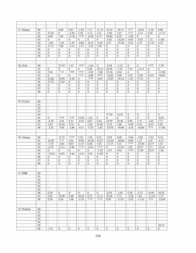
154
27. Manny 00 - 0.88 0.87 -2.59 1.77 11.74 34.19 -36.31 -24.77 -18.01 -5.30 8.00 01 31.85 0 -4.49 5.29 1.12 3.31 -1.60 1.63 -25.13 -2.14 5.84 -11.72 02 4.69 7.46 17.36 -14.20 -8.28 0.75 30.60 6.29 -2.69 0 0 0 03 0 0 0 0 0 0 -4.42 -24.28 -6.87 -4.92 1.72 11.86 04 -3.03 -7.81 -3.39 -0.88 -8.74 -6.38 2.27 -15.56 -9.21 4.35 27.78 4.35 05 17.71 7.08 -3.31 -1.71 -5.22 5.50 0 0 0 0 0 0 06 0 0 0 0 0 0 0 0 0 0 0 0 07 0 0 0 0 0 0 0 0 0 0 0 0 08 0 0 0 0 0 0 0 0 0 0 0 0 28. NAL 00 - 23.39 1.12 -10.29 -1.64 0 -9.58 -3.23 0 0 -19.22 -7.59 01 0 0 0 0 0.48 70.14 49.58 -3.54 7.53 -12.21 0 0 02 3.56 -13.23 -10.06 -15.93 -2.02 -7.00 53.10 6.94 0 0 0 -12.90 03 0 0 0 -13.51 -4.06 -30.29 -14.02 5.98 1.03 -5.58 41.81 -36.65 04 21.60 39.09 -4.38 0 -12.98 -9.65 -15.05 -25.14 -1.53 37.21 0 0 05 37.74 27.85 0 0 0 0 0 0 0 0 0 0 06 0 0 0 0 0 0 0 0 0 0 0 0 07 0 0 0 0 0 0 0 0 0 0 0 0 08 0 0 0 0 0 0 0 0 0 0 0 0 29. Oceanic 00 - - - - - - - - - - - - 01 - - - - - - - - - - - - 02 - - - - - - - - - - - - 03 - - - - - - - - - - - - 04 - - - - - - 37.50 14.55 0 0 0 0 05 0 -14.60 -12.83 33.05 1.28 0 0 0 0 0 0 -0.63 06 -4.78 -3.01 9.14 -0.16 8.07 6.44 19.39 38.48 8.99 7.33 -2.42 5.17 07 2.43 25.44 5.34 0 1.49 41.62 -2.14 3.68 -0.46 9.14 -6.53 6.92 08 -2.52 -3.65 -2.86 -0.71 -5.25 -2.45 -10.70 -19.98 -4.16 -16.86 -29.31 -17.66 30. Omega 00 - 12.75 -14.78 2.55 1.49 8.33 -9.50 6.00 -5.66 -4.50 -2.62 9.14 01 14.29 -11.21 2.91 -0.94 34.29 32.27 -15.28 -24.68 -0.84 1.27 1.67 -6.17 02 -1.75 -4.02 0.93 -4.15 0.48 1.91 -13.15 5.41 -13.33 -35.50 24.77 1.47 03 -4.35 12.12 -9.46 -17.16 14.41 -13.39 0 -11.82 1.03 28.57 8.73 13.14 04 0 0 0 0 0 -7.10 -3.47 5.04 -22.60 11.50 29.37 -1.84 05 -15.63 14.07 -5.84 12.41 5.52 11.05 0 0 0 0 0 0 06 0 0 0 0 0 0 0 0 0 0 0 0 07 0 0 0 0 0 0 0 0 0 0 0 0 08 0 0 0 0 0 0 0 0 0 0 0 0 31. PHB 00 - - - - - - - - - - - - 01 - - - - - - - - - - - - 02 - - - - - - - - - - - - 03 - - - - - - - - - - - - 04 - - - - - - - - - - - - 05 - - - - - - - - - - - - 06 0.39 0 0 0 0 0 -6.54 -1.65 6.28 -5.12 14.94 16.25 07 0.62 53.09 9.48 29.65 0.35 32.11 25.68 3.73 -2.28 7.64 -11.10 -7.37 08 9.26 9.26 1.06 -5.19 -31.87 -23.16 0.99 -13.97 -2.82 -11.45 -18.42 -22.04 32. Prudent 00 - - - - - - - - - - - - 01 - - - - - - - - - - - - 02 - - - - - - - - - - - - 03 - - - - - - - - - - - - 04 - - - - - - - - - - - - 05 - - - - - - - - - - - 30.74 06 1.32 0 0 0 0 0 0 0 0 0 0 0

155
07 0 0 0 0 0 0 0 0 0 0 0 0 08 0 0 0 0 0 0 0 0 0 0 0 0 33. Regent 00 - - - - - - - - - - - - 01 - - - - - - - - - - - - 02 - - - - - - - - - - - - 03 - - - - - - - - 0 72.06 -1.71 -10.43 04 1.94 12.38 -1.69 -3.45 -9.82 -0.99 -5.00 -4.21 0 0 -5.49 -1.16 05 -3.53 -1.22 0 0 0 0 0 0 2.47 7.23 0 0 06 0 0 0 0 0 0 0 0 0 0 0 0 07 0 0 0 0 0 0 0 0 0 0 0 0 08 0 0 0 0 0 0 0 0 0 0 0 0 34. Savannah 00 - 6.36 -12.82 7.84 6.36 9.40 15.63 10.14 10.43 -10.27 -4.58 3.20 01 20.16 -2.58 -2.65 -12.93 1.56 -3.08 -3.17 4.10 -1.57 8.00 -12.59 -13.56 02 -6.86 -14.74 -1.23 0 0 0 0 0 0 0 0 0 03 0 0 0 0 0 0 0 0 0 0 0 0 04 0 0 0 0 0 0 0 0 0 0 0 05 0 0 0 0 0 0 0 0 0 0 0 0 06 0 0 0 0 0 0 0 0 0 0 0 0 07 0 0 0 0 0 0 0 0 0 0 0 0 08 0 0 0 0 0 0 0 0 0 0 0 0 35. Skye 00 - - - - - - - - - - - - 01 - - - - - - - - - - - - 02 - - - - - - - - - - - - 03 - - - - - - - - - - - - 04 - - - - - - - - - - - - 05 - - - - - - - - - - - - 06 - - - - - - - - - - 0 -18.97 07 -16.81 50.13 0 20.61 17.37 44.89 5.40 -1.26 8.54 9.93 7.36 -64.30 08 196.16 -0.77 1.48 4.39 -8.91 5.85 -13.55 -15.67 3.11 -17.09 -8.86 -9.62 36. Spring 00 - - - - - - - - - - - - 01 - - - - - - - - - - - - 02 - - - - - - - - - - - - 03 - - - - - - - - - - - - 04 - - - - - - - - - - - - 05 - - - - - - - - - - - - 06 - - - - - - - - - - - 0.56 07 -25.14 -6.72 11.80 0 0 0 0 0 0 0 0 0 08 0 0 0 0 50.98 -33.77 0 0 0 0 0 0 37. Sterling 00 - - - - - - - - - - - - 01 - - - - - - - - - - - - 02 - - - - - - - - - - - - 03 - - - - - - - - - - - - 04 - - - - - - - - - - - - 05 - - - - - - - - - - - - 06 - - - - - - - - 0 127.14 -16.35 -18.42 07 -20.51 29.28 -3.14 27.08 19.67 35.31 -8.32 -3.31 -1.65 -5.42 -0.82 -0.14 08 0 0 0 0 2.88 -10.55 -0.30 -0.45 -11.28 -16.27 -24.49 -31.37 38. STB 00 - - - - - - - - - - - - 01 - - - - - - - - - - - - 02 - - - - - - - - - - - - 03 - - - - - - - - 0 72.06 -1.71 -10.43 04 - - 0 55.93 -0.86 -14.76 -15.28 -4.41 -9.64 9.28 33.33 17.99
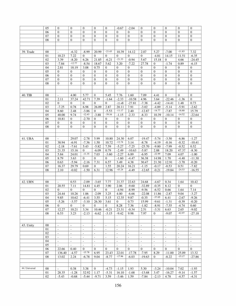
156
05 0 0 0 0 0 -0.67 -2.04 0 0 0 0 0 06 0 0 0 0 0 0 0 0 0 0 0 0 07 0 0 0 0 0 0 0 0 0 0 0 0 08 0 0 0 0 0 0 0 0 0 0 0 0 39. Trade 00 - -6.32 -8.99 20.99 -21.43 10.39 14.12 2.07 5.27 -7.00 -11.83 7.32 01 10.23 7.22 0 0 0 0 0 0 -4.81 14.15 11.51 -6.35 02 3.39 -8.20 6.26 21.85 -6.21 -21.33 -0.94 5.67 15.18 0 4.66 -24.45 03 -7.84 -12.77 -8.54 18.67 5.62 3.20 -7.22 27.78 0 -1.74 0.89 -6.15 04 2.81 18.19 3.08 0.75 0 0 0 0 0 0 0 0 05 0 0 0 0 0 0 0 0 0 0 0 0 06 0 0 0 0 0 0 0 0 0 0 0 0 07 0 0 0 0 0 0 0 0 0 0 0 0 08 0 0 0 0 0 0 0 0 0 0 0 0 40. TIB 00 - 4.00 5.77 0 5.45 7.76 1.60 7.09 4.41 0 0 0 01 2.11 37.24 42.71 7.39 -1.64 -2.33 -10.58 4.96 3.64 -22.46 -1.36 0 02 0 0 0 0 0 -22.48 -27.81 -7.38 -4.42 -14.41 1.48 0.73 03 -7.25 0.78 6.98 26.09 2.87 20.11 7.91 -3.02 -4.89 -5.14 -5.91 -2.62 04 8.60 2.48 -3.86 0 -5.53 -11.17 2.40 -12.87 -14.77 -7.87 -18.80 15.79 05 40.00 9.74 -12.43 -3.88 -39.16 -1.15 -2.33 -8.33 10.39 -10.14 -14.52 -22.64 06 10.81 0 -2.70 0 0 0 0 0 0 0 0 0 07 0 0 0 0 0 0 0 0 0 0 0 0 08 0 0 0 0 0 0 0 0 0 0 0 0 41. UBA 00 - 29.07 -2.78 5.99 10.80 24.30 6.07 -19.47 -5.74 -3.50 -6.86 -1.27 01 38.94 -6.91 -7.36 1.50 10.72 -12.74 3.14 -8.78 -4.19 -0.16 -0.32 -10.41 02 -2.18 -7.61 5.43 -5.82 7.59 -5.27 -7.25 -25.70 -9.80 -7.99 -0.52 0.52 03 21.35 15.16 0 -6.09 0.79 -2.49 -10.63 -5.87 2.88 18.20 47.37 -8.30 04 5.84 24.01 -11.35 7.03 -3.60 -2.27 6.89 -6.95 -22.99 7.09 4.07 -1.00 05 8.79 3.63 0 0 0 -1.60 -4.47 36.38 14.98 1.70 -4.40 -11.30 06 0.63 -5.94 -2.16 7.31 6.57 3.49 4.38 30.47 21.30 12.91 -3.70 -0.20 07 16.37 29.79 0.69 0 1.55 20.24 16.21 -1.15 -0.17 -0.53 0.51 -7.82 08 2.10 -0.02 -1.50 6.31 12.96 -43.24 -4.49 -12.65 -0.21 -19.84 -24.53 -16.55 42. UBN 00 - 0.53 -2.09 -3.65 7.77 21.37 22.63 24.68 -4.67 0.34 1.64 10.42 01 20.55 7.11 14.81 4.45 3.90 2.06 -9.60 -32.89 -0.35 8.12 0 0 02 0 0 0 0 0 -4.94 -8.99 -9.56 -6.52 0.66 1.64 7.14 03 24.44 10.26 1.06 -2.09 3.25 4.00 -6.66 -22.08 11.86 -2.87 9.04 -3.27 04 9.85 10.62 -6.41 3.55 5.15 12.35 9.87 -0.35 -37.05 6.41 -2.67 -9.26 05 -5.26 -3.57 -3.10 26.30 3.61 0 0.73 15.99 -9.61 -1.31 -0.39 -0.20 06 0 0 0 0 0 8.28 7.36 -1.82 -8.91 -7.55 -4.74 0.60 07 12.27 10.21 3.34 10.46 -0.21 23.31 -0.34 2.51 -3.31 6.63 2.65 -9.02 08 6.53 3.23 -2.13 -6.62 -3.15 -9.42 9.98 7.97 0 -9.07 -42.97 -27.18 43. Unity 00 - - - - - - - - - - - - 01 - - - - - - - - - - - - 02 - - - - - - - - - - - - 03 - - - - - - - - - - - - 04 - - - - - - - - - - - - 05 - - - - - - - - - - - - 06 22.66 0.40 0 0 0 0 0 0 0 0 0 0 07 136.40 -4.57 -15.78 6.95 23.43 22.01 -17.78 -7.95 8.29 -11.00 25.09 13.32 08 13.02 2.24 -6.78 9.04 -8.77 -17.96 -6.03 -19.63 0 -8.22 -15.17 -27.86 44. Universal 00 - 0.38 3.38 0 -4.73 -1.15 1.93 5.30 -3.24 -10.04 7.02 -1.93 01 28.35 -1.28 32.92 1.17 -5.31 16.10 -1.68 -13.68 3.47 -16.27 -9.14 -1.57 02 -5.43 -0.68 -5.44 -9.71 3.59 -3.46 1.59 -7.84 -2.13 4.78 -4.57 -4.31
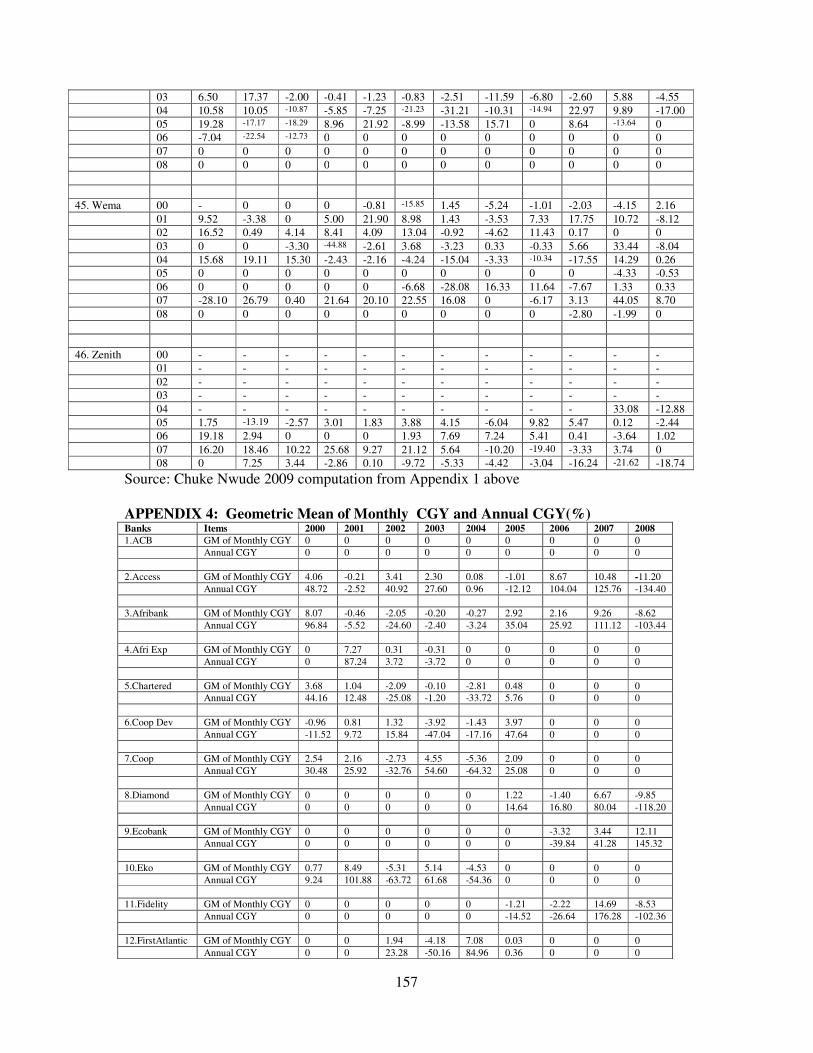
157
03 6.50 17.37 -2.00 -0.41 -1.23 -0.83 -2.51 -11.59 -6.80 -2.60 5.88 -4.55 04 10.58 10.05 -10.87 -5.85 -7.25 -21.23 -31.21 -10.31 -14.94 22.97 9.89 -17.00 05 19.28 -17.17 -18.29 8.96 21.92 -8.99 -13.58 15.71 0 8.64 -13.64 0 06 -7.04 -22.54 -12.73 0 0 0 0 0 0 0 0 0 07 0 0 0 0 0 0 0 0 0 0 0 0 08 0 0 0 0 0 0 0 0 0 0 0 0 45. Wema 00 - 0 0 0 -0.81 -15.85 1.45 -5.24 -1.01 -2.03 -4.15 2.16 01 9.52 -3.38 0 5.00 21.90 8.98 1.43 -3.53 7.33 17.75 10.72 -8.12 02 16.52 0.49 4.14 8.41 4.09 13.04 -0.92 -4.62 11.43 0.17 0 0 03 0 0 -3.30 -44.88 -2.61 3.68 -3.23 0.33 -0.33 5.66 33.44 -8.04 04 15.68 19.11 15.30 -2.43 -2.16 -4.24 -15.04 -3.33 -10.34 -17.55 14.29 0.26 05 0 0 0 0 0 0 0 0 0 0 -4.33 -0.53 06 0 0 0 0 0 -6.68 -28.08 16.33 11.64 -7.67 1.33 0.33 07 -28.10 26.79 0.40 21.64 20.10 22.55 16.08 0 -6.17 3.13 44.05 8.70 08 0 0 0 0 0 0 0 0 0 -2.80 -1.99 0 46. Zenith 00 - - - - - - - - - - - - 01 - - - - - - - - - - - - 02 - - - - - - - - - - - - 03 - - - - - - - - - - - - 04 - - - - - - - - - - 33.08 -12.88 05 1.75 -13.19 -2.57 3.01 1.83 3.88 4.15 -6.04 9.82 5.47 0.12 -2.44 06 19.18 2.94 0 0 0 1.93 7.69 7.24 5.41 0.41 -3.64 1.02 07 16.20 18.46 10.22 25.68 9.27 21.12 5.64 -10.20 -19.40 -3.33 3.74 0 08 0 7.25 3.44 -2.86 0.10 -9.72 -5.33 -4.42 -3.04 -16.24 -21.62 -18.74
Source: Chuke Nwude 2009 computation from Appendix 1 above APPENDIX 4: Geometric Mean of Monthly CGY and Annual CGY(%) Banks Items 2000 2001 2002 2003 2004 2005 2006 2007 2008 1.ACB GM of Monthly CGY 0 0 0 0 0 0 0 0 0 Annual CGY 0 0 0 0 0 0 0 0 0 2.Access GM of Monthly CGY 4.06 -0.21 3.41 2.30 0.08 -1.01 8.67 10.48 -11.20 Annual CGY 48.72 -2.52 40.92 27.60 0.96 -12.12 104.04 125.76 -134.40 3.Afribank GM of Monthly CGY 8.07 -0.46 -2.05 -0.20 -0.27 2.92 2.16 9.26 -8.62 Annual CGY 96.84 -5.52 -24.60 -2.40 -3.24 35.04 25.92 111.12 -103.44 4.Afri Exp GM of Monthly CGY 0 7.27 0.31 -0.31 0 0 0 0 0 Annual CGY 0 87.24 3.72 -3.72 0 0 0 0 0 5.Chartered GM of Monthly CGY 3.68 1.04 -2.09 -0.10 -2.81 0.48 0 0 0 Annual CGY 44.16 12.48 -25.08 -1.20 -33.72 5.76 0 0 0 6.Coop Dev GM of Monthly CGY -0.96 0.81 1.32 -3.92 -1.43 3.97 0 0 0 Annual CGY -11.52 9.72 15.84 -47.04 -17.16 47.64 0 0 0 7.Coop GM of Monthly CGY 2.54 2.16 -2.73 4.55 -5.36 2.09 0 0 0 Annual CGY 30.48 25.92 -32.76 54.60 -64.32 25.08 0 0 0 8.Diamond GM of Monthly CGY 0 0 0 0 0 1.22 -1.40 6.67 -9.85 Annual CGY 0 0 0 0 0 14.64 16.80 80.04 -118.20 9.Ecobank GM of Monthly CGY 0 0 0 0 0 0 -3.32 3.44 12.11 Annual CGY 0 0 0 0 0 0 -39.84 41.28 145.32 10.Eko GM of Monthly CGY 0.77 8.49 -5.31 5.14 -4.53 0 0 0 0 Annual CGY 9.24 101.88 -63.72 61.68 -54.36 0 0 0 0 11.Fidelity GM of Monthly CGY 0 0 0 0 0 -1.21 -2.22 14.69 -8.53 Annual CGY 0 0 0 0 0 -14.52 -26.64 176.28 -102.36 12.FirstAtlantic GM of Monthly CGY 0 0 1.94 -4.18 7.08 0.03 0 0 0 Annual CGY 0 0 23.28 -50.16 84.96 0.36 0 0 0
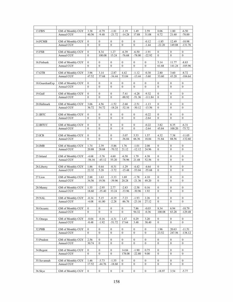
158
13.FBN GM of Monthly CGY 3.38 -0.79 -1.81 -1.19 1.49 2.59 0.06 1.80 -6.50 Annual CGY 40.56 -9.48 -21.72 -14.28 17.88 31.08 0.72 21.60 -78.00 14.FCMB GM of Monthly CGY 0 0 0 0 0 -0.12 -1.85 12.49 -10.98 Annual CGY 0 0 0 0 0 -1.44 -22.20 149.88 -131.76 15.FSB GM of Monthly CGY 0 8.34 1.27 -6.39 -6.50 -1.91 0 0 0 Annual CGY 0 100.08 15.24 -76.68 -78.00 -22.92 0 0 0 16.Finbank GM of Monthly CGY 0 0 0 0 0 0 5.14 11.77 -8.83 Annual CGY 0 0 0 0 0 0 61.68 141.24 -105.96 17.GTB GM of Monthly CGY 3.96 3.14 -2.87 4.42 -1.12 -0.30 2.80 3.60 -8.72 Annual CGY 47.52 37.68 -34.44 53.04 -13.44 -3.60 33.60 43.20 -104.64 18.GuardianExp GM of Monthly CGY 0 0 0 0 0 0 0 0 0 Annual CGY 0 0 0 0 0 0 0 0 0 19.Gulf GM of Monthly CGY 0 0 0 -7.41 -4.28 -9.32 0 0 0 Annual CGY 0 0 0 -88.92 -51.36 -111.84 0 0 0 20.Hallmark GM of Monthly CGY 3.06 4.56 -1.52 -2.68 -2.51 -1.13 0 0 0 Annual CGY 36.72 54.72 -18.24 -32.16 -30.12 -13.56 0 0 0 21.IBTC GM of Monthly CGY 0 0 0 0 0 -0.22 0 0 0 Annual CGY 0 0 0 0 0 -2.64 0 0 0 22.IBTCC GM of Monthly CGY 0 0 0 0 0 -0.22 3.82 8.35 -6.31 Annual CGY 0 0 0 0 0 -2.64 45.84 100.20 -75.72 23.ICB GM of Monthly CGY 0 0 0 -3.07 5.53 1.57 4.32 7.38 -11.05 Annual CGY 0 0 0 -36.84 66.36 18.84 51.84 88.56 -132.60 24.IMB GM of Monthly CGY 1.74 2.39 -5.86 1.76 -1.01 2.08 0 0 0 Annual CGY 20.88 28.68 -70.32 21.12 -12.12 24.96 0 0 0 25.Inland GM of Monthly CGY -4.68 -3.76 4.60 -6.58 1.79 4.38 0 0 0 Annual CGY -56.16 -45.12 55.20 -78.96 21.48 52.56 0 0 0 26.Liberty GM of Monthly CGY 1.86 0.44 -0.31 -1.29 -4.42 -4.64 0 0 0 Annual CGY 22.32 5.28 -3.72 -15.48 -53.04 -55.68 0 0 0 27.Lion GM of Monthly CGY 2.88 1.63 -3.33 1.69 -1.78 4.10 0 0 0 Annual CGY 34.56 19.56 -39.96 20.28 -21.36 49.20 0 0 0 28.Manny GM of Monthly CGY 1.55 -2.95 2.77 -2.83 -2.58 0.16 0 0 0 Annual CGY 18.60 -35.40 33.24 -33.96 -30.96 1.92 0 0 0 29.NAL GM of Monthly CGY -0.34 5.15 -0.19 -7.23 -1.93 2.26 0 0 0 Annual CGY -4.08 61.80 -2.28 -86.76 -23.16 27.12 0 0 0 30.Oceanic GM of Monthly CGY 0 0 0 0 7.86 -0.03 8.34 6.94 -10.79 Annual CGY 0 0 0 0 94.32 -0.36 100.08 83.28 -129.48 31.Omega GM of Monthly CGY -0.04 -0.16 -4.31 1.47 0.29 3.20 0 0 0 Annual CGY -0.48 -1.92 -51.72 17.64 3.48 38.40 0 0 0 32.PHB GM of Monthly CGY 0 0 0 0 0 0 1.96 20.63 -11.51 Annual CGY 0 0 0 0 0 0 23.52 247.56 -138.12 33.Prudent GM of Monthly CGY 2.56 0 0 0 0 0 0 0 0 Annual CGY 30.74 0 0 0 0 0 0 0 0 34.Regent GM of Monthly CGY 0 0 0 14.84 -1.90 0.75 0 0 0 Annual CGY 0 0 0 178.08 -22.80 9.00 0 0 0 35.Savannah GM of Monthly CGY 1.46 -3.73 -1.55 0 0 0 0 0 0 Annual CGY 17.52 -44.76 -18.60 0 0 0 0 0 0 36.Skye GM of Monthly CGY 0 0 0 0 0 0 -18.97 3.54 -5.77

159
Annual CGY 0 0 0 0 0 0 -227.64 42.48 -69.24 37.Spring GM of Monthly CGY 0 0 0 0 0 0 -0.56 0.38 0 Annual CGY 0 0 0 0 0 0 -6.72 4.56 0 38.Sterling GM of Monthly CGY 0 0 0 0 0 0 15.73 7.02 -9.06 Annual CGY 0 0 0 0 0 0 15.73 84.24 -108.72 39.STB GM of Monthly CGY 0 0 0 0 5.78 -0.45 0 0 0 Annual CGY 0 0 0 0 69.36 -5.40 0 0 0 40.Trade GM of Monthly CGY -0.69 1.80 -1.61 1.18 1.88 0 0 0 0 Annual CGY -8.28 21.60 -19.32 14.16 22.56 0 0 0 0 41.TIB GM of Monthly CGY 3.24 3.78 -4.07 3.46 -5.38 -11.34 -0.30 0 0 Annual CGY 38.88 45.36 -48.84 41.52 -64.56 -136.08 -3.60 0 0 42.UBA GM of Monthly CGY 2.48 -3.45 -5.53 3.56 -1.83 2.54 6.27 4.87 -10.87 Annual CGY 29.76 -41.40 -66.36 42.72 -21.96 30.48 75.24 58.44 -130.44 43.UBN GM of Monthly CGY 6.68 -1.05 -1.99 -0.22 -1.79 1.90 -0.74 3.90 -8.62 Annual CGY 80.16 -12.60 -23.88 -2.64 -21.48 22.80 -8.88 46.80 -103.44 44.Unity GM of Monthly CGY 0 0 0 0 0 0 0.04 2.69 -11.07 Annual CGY 0 0 0 0 0 0 0.48 32.28 -132.84 45.Universal GM of Monthly CGY -0.38 -0.37 -3.50 -1.08 -8.05 -2.37 -3.50 0 0 Annual CGY -4.56 -4.44 -42.00 -12.96 -96.60 -28.44 -42.00 0 0 46.Wema GM of Monthly CGY -2.44 4.92 3.16 -3.51 -1.22 -0.45 -1.81 12.97 -0.44 Annual CGY -29.28 59.04 37.92 -42.12 -14.64 -5.40 -21.72 155.64 -5.28 47.Zenith GM of Monthly CGY 0 0 0 0 7.68 0.18 2.04 4.74 -7.08 Annual CGY 0 0 0 0 92.16 2.16 24.48 56.88 -84.96
Source: Chuke Nwude 2009 computation from Appendix 2 above APPENDIX 5 : Dividend Yields (%) Banks Items 2000 2001 2002 2003 2004 2005 2006 2007 2008 1.ACB Dividend
Yield 0 0 0 0 0 0 - - -
2.Access Dividend
Yield�5.36 0 0 1.94 3.40 0 0 2.09
3.Afribank Dividend
Yield�0 1.70 1.30 2.16 3.01 0 0 0.97
4.Afri Exp Dividend
Yield�0 0 0 0 0 0 0 0 -
5.Chartered Dividend
Yield 5.34 2.62 8.36 8.22 8.47 0 - - -
6.Coop Dev Dividend 11.11 0 0 5.98 0 0 - - -

160
Yield 7.Coop Dividend
Yield 8.67 0 0 7.63 0 0 - - -
8.Diamond Dividend
Yield - - - - - 0 0 2.95
9.Ecobank Dividend
Yield - - - - - 1.22 1.16 2.55
10.Eko Dividend
Yield 7.69 4.38 - 0 7.62 0 - - -
11.Fidelity Dividend
Yield - - - - - 0 4.80 1.33
12.FirstAtlantic Dividend
Yield
13.FBN Dividend
Yield 8.26 4.60 5.28 6.08 6.33 5.77 1.94 2.11 3.76
14.FCMB Dividend
Yield - - - - 0.76 1.47 2.73 1.97 3.98
15.FSB Dividend
Yield 10.29 8.57 3.27 0 0 - - - -
16.Finbank Dividend
Yield - - 6.17 7.08 0 0 0 0 0
17.GTB Dividend
Yield 3.10 10.86 11.93 9.69 5.33 7.25 6.85 2.50
18.GuardianExp Dividend
Yield - - - - - - - - -

161
19.Gulf Dividend
Yield - - - - - - - - -
20.Hallmark Dividend
Yield 15.63 1.76 0 0 0 - - - -
21.IBTC Dividend
Yield - - - - - - - - -
22.IBTCC Dividend
Yield - - - - - 4.38 3.19 2.80
23.ICB Dividend
Yield - - - - - 7.04 3.86 2.39 3.10
24.IMB Dividend
Yield 0 0 0 0 0 0 - - -
25.Inland Dividend
Yield 0 0 18.61 3.72 0 0 - - -
26.Liberty Dividend
Yield - - - - - - - - -
27.Lion Dividend
Yield 13.64 8.70 3.70 7.27 - - - - -
28.Manny Dividend
Yield 8.62 2.94 2.96 0 2.63 - - - -
29.NAL Dividend
Yield - - - - - - - - -
30.Oceanic Dividend
Yield - - - - 4.65 5.10 2.84 3.38

162
31.Omega Dividend
Yield 6.16 7.46 12.32 0 0 6.54 - - -
32.PHB Dividend
Yield - - - - - 0 2.02 2.26
33.Prudent Dividend
Yield - - - - - - - - -
34.Regent Dividend
Yield - - - - - - - - -
35.Savannah Dividend
Yield - - - - - - - - -
36.Skye Dividend
Yield - - - - - 0 0 2.06
37.Spring Dividend
Yield - - - - - 0 0 0 0
38.Sterling Dividend
Yield - - - - - 0 0 0 0
39.STB Dividend
Yield - - - - - - - - -
40.Trade Dividend
Yield 0 9.62 8.40 0 - - - - -
41.TIB Dividend
Yield 0 0 10.87 5.38 0 - - - -
42.UBA Dividend
Yield 4.91 1.77 3.21 6.78 5.35 6.38 3.44 2.40 7.08

163
43.UBN Dividend Yield
5.91 4.35 6.41 4.97 3.79 4.87 3.44 2.27 4.59
44.Unity Dividend
Yield - - - - - 2.46 0 0
45.Universal Dividend
Yield - - - - - - - - -
46.Wema Dividend
Yield 7.77 8.53 8.74 7.99 2.41 0 0 0 0
47.Zenith Dividend
Yield - - - - 5.26 4.95 4.76 1.75 4.28
Source: Chuke Nwude 2009 computation from the Banks’ Annual Reports and Accounts APPENDIX 6: Stocks Actual Annual Rates of Return(%) Banks Items 2000 2001 2002 2003 2004 2005 2006 2007 2008 1.ACB GM of Monthly CGY 0 0 0 0 0 0 - - - Annual CGY 0 0 0 0 0 0 - - - Dividend Yield 0 0 0 0 0 0 - - - ������������ 0 0 0 0 0 0 - - - 2.Access GM of Monthly CGY 4.06 -0.21 3.41 2.30 0.08 -1.01 8.67 10.48 -11.20 Annual CGY 48.72 -2.52 40.92 27.60 0.96 -12.12 104.04 125.76 -134.40 Dividend Yield� 5.36 0 0 1.94 3.40 0 0 2.09 ����������� 54.08 -2.52 40.92 29.54 4.36 -12.12 104.04 127.85 3.Afribank GM of Monthly CGY 8.07 -0.46 -2.05 -0.20 -0.27 2.92 2.16 9.26 -8.62 Annual CGY 96.84 -5.52 -24.60 -2.40 -3.24 35.04 25.92 111.12 -103.44 Dividend Yield 0 1.70 1.30 2.16 3.01 0 0 0.97
������������ 96.84 -3.82 -23.30 -0.24 -0.23 35.04 25.92 112.09
4.Afri Exp GM of Monthly CGY 0 7.27 0.31 -0.31 0 0 - - - Annual CGY 0 87.24 3.72 -3.72 0 0 - - - Dividend Yield 0 0 0 0 0 0 - - -
������������ 0 87.24 3.72 -3.72 0 0 - - -
5.Chartered GM of Monthly CGY 3.68 1.04 -2.09 -0.10 -2.81 0.48 - - - Annual CGY 44.16 12.48 -25.08 -1.20 -33.72 5.76 - - - Dividend Yield 5.34 2.62 8.36 8.22 8.47 0 - - -
������������ 49.50 15.10 -16.72 7.02 -25.25 5.76 - - -
6.Coop Dev GM of Monthly CGY -0.96 0.81 1.32 -3.92 -1.43 3.97 - - - Annual CGY -11.52 9.72 15.84 -47.04 -17.16 47.64 - - - Dividend Yield 11.11 0 0 5.98 0 0 - - -
������������ -0.41 9.72 15.84 -41.06 -17.16 47.64 - - -
7.Coop GM of Monthly CGY 2.54 2.16 -2.73 4.55 -5.36 2.09 - - - Annual CGY 30.48 25.92 -32.76 54.60 -64.32 25.08 - - - Dividend Yield 8.67 0 0 7.63 0 0 - - --
������������ 39.15 25.92 -32.76 62.23 -64.32 25.08 - - -

164
8.Diamond GM of Monthly CGY - - - - - 1.22 -1.40 6.67 -9.85 Annual CGY - - - - - 14.64 16.80 80.04 -118.20 Dividend Yield - - - - - 0 0 2.95
������������ - - - - - 14.64 16.80 82.99
9.Ecobank GM of Monthly CGY - - - - - - -3.32 3.44 12.11 Annual CGY - - - - - - -39.84 41.28 145.32 Dividend Yield - - - - - 1.22 1.16 2.55
������������ - - - - - 1.22 -38.68 43.83
10.Eko GM of Monthly CGY 0.77 8.49 -5.31 5.14 -4.53 - - - - Annual CGY 9.24 101.88 -63.72 61.68 -54.36 - - - - Dividend Yield 7.69 4.38 0 0 7.62 - - - -
������������ 16.93 106.26 -63.72 61.68 -46.74 - - - -
11.Fidelity GM of Monthly CGY - - - - - -1.21 -2.22 14.69 -8.53 Annual CGY - - - - -- -14.52 -26.64 176.28 -102.36 Dividend Yield - - - - - 0 4.80 1.33
������������ - - - - - -14.52 -21.84 177.61
12.FirstAtlantic GM of Monthly CGY - - 1.94 -4.18 7.08 0.03 - - - Annual CGY - - 23.28 -50.16 84.96 0.36 - - - Dividend Yield - - - - - - - - -
������������ - - 23.28 -50.16 84.96 0.36 - - -
13.FBN GM of Monthly CGY 3.38 -0.79 -1.81 -1.19 1.49 2.59 0.06 1.80 -6.50 Annual CGY 40.56 -9.48 -21.72 -14.28 17.88 31.08 0.72 21.60 -78.00 Dividend Yield 8.26 4.60 5.28 6.08 6.33 5.77 1.94 2.11 3.76
������������ 48.82 -4.88 -16.44 -8.20 24.21 36.85 2.66 23.71 -74.24
14.FCMB GM of Monthly CGY - - - - -- -0.12 -1.85 12.49 -10.98 Annual CGY - - - - - -1.44 -22.20 149.88 -131.76 Dividend Yield - - - - - 1.47 2.73 1.97 3.98
������������ - - - - - 0.03 -19.47 151.85 135.74
15.FSB GM of Monthly CGY 0 8.34 1.27 -6.39 -6.50 -1.91 - - - Annual CGY 0 100.08 15.24 -76.68 -78.00 -22.92 - - - Dividend Yield 10.29 8.57 3.27 - - - - - -
������������ 10.29 108.65 18.51 -76.68 -78.00 -22.92 - - -
16.Finbank GM of Monthly CGY - - - - - - 5.14 11.77 -8.83 Annual CGY - - - - - - 61.68 141.24 -105.96 Dividend Yield - - - - - - 0 0 0
������������ - - - - - - 61.68 141.24 -105.96
17.GTB GM of Monthly CGY 3.96 3.14 -2.87 4.42 -1.12 -0.30 2.80 3.60 -8.72 Annual CGY 47.52 37.68 -34.44 53.04 -13.44 -3.60 33.60 43.20 -104.64 Dividend Yield 3.10 4.87 11.93 9.69 5.33 4.54 5.43 2.50
������������ 50.62 42.55 -22.51 62.73 -8.11 0.94 39.03 45.70
18.GuardianExp GM of Monthly CGY 0 0 0 0 0 0 - - - Annual CGY 0 0 0 0 0 0 - - - Dividend Yield 0 0 0 0 0 0 - - -
������������ 0 0 0 0 0 0 - - -
19.Gulf GM of Monthly CGY - - - -7.41 -4.28 -9.32 - - - Annual CGY - - - -88.92 -51.36 -111.84 - - - Dividend Yield - - - - - - - - -

165
������������ - - - -88.92 -51.36 -111.84 - - -
20.Hallmark GM of Monthly CGY 3.06 4.56 -1.52 -2.68 -2.51 -1.13 - - - Annual CGY 36.72 54.72 -18.24 -32.16 -30.12 -13.56 - - - Dividend Yield 15.63 1.76 0 0 0 0 - - -
������������ 52.35 56.48 -18.24 -32.16 -30.12 -13.56 - - -
21.IBTC GM of Monthly CGY - - - - - -0.22 - - - Annual CGY - - - - - -2.64 -- - - Dividend Yield - - - - - 0 - - --
������������ - - - - -- -2.64 - - -
22.IBTCC GM of Monthly CGY - - - - - -0.22 3.82 8.35 -6.31 Annual CGY - -- - - -- -2.64 45.84 100.20 -75.72 Dividend Yield - - - - - 4.38 3.19 2.80
������������ - - - - -- 1.74 49.03 103.00
23.ICB GM of Monthly CGY -- - - -3.07 5.53 1.57 4.32 7.38 -11.05 Annual CGY - - -- -36.84 66.36 18.84 51.84 88.56 -132.60 Dividend Yield - - - - - 7.04 3.86 2.39 3.10
������������ - - - - -- 25,88 55.70 90.95 -129.50
24.IMB GM of Monthly CGY 1.74 2.39 -5.86 1.76 -1.01 2.08 - - - Annual CGY 20.88 28.68 -70.32 21.12 -12.12 24.96 - - - Dividend Yield 0 0 0 0 0 0
������������ 20.88 28.68 -70.32 21.12 -12.12 24.96 - - -
25.Inland GM of Monthly CGY -4.68 -3.76 4.60 -6.58 1.79 4.38 - - - Annual CGY -56.16 -45.12 55.20 -78.96 21.48 52.56 - - - Dividend Yield 0 0 18.61 3.72 0 0 - - -
������������ -56.16 -45.12 73.81 -75.24 21.48 52.56 - - -
26.Liberty GM of Monthly CGY 1.86 0.44 -0.31 -1.29 -4.42 -4.64 - - - Annual CGY -56.16 -45.12 -56.16 -45.12 -56.16 -45.12 - - - Dividend Yield - - - - - - - - -
������������ -56.16 -45.12 -56.16 -45.12 -56.16 -45.12 - - -
27.Lion GM of Monthly CGY 2.88 1.63 -3.33 1.69 -1.78 4.10 - - - Annual CGY 34.56 19.56 -39.96 20.28 -21.36 49.20 - - - Dividend Yield - - - - - - - - -
������������ 34.56 19.56 -39.96 20.28 -21.36 49.20 - - -
28.Manny GM of Monthly CGY 1.55 -2.95 2.77 -2.83 -2.58 0.16 - - - Annual CGY 18.60 -35.40 33.24 -33.96 -30.96 1.92 - - - Dividend Yield - - - - - - - - -
������������ 18.60 -35.40 33.24 -33.96 -30.96 1.92 - - -
29.NAL GM of Monthly CGY -0.34 5.15 -0.19 -7.23 -1.93 2.26 - - - Annual CGY -4.08 61.80 -2.28 -86.76 -23.16 27.12 - - - Dividend Yield - - - - - - - - -
������������ -4.08 61.80 -2.28 -86.76 -23.16 27.12 - - -
30.Oceanic GM of Monthly CGY - - - - 7.86 -0.03 8.34 6.94 -10.79 Annual CGY - - - - 94.32 -0.36 100.08 83.28 -129.48 Dividend Yield - - - - 4.65 5.10 2.84 3.38
������������ - - - - 98.97 4.74 102.92 86.66
31.Omega GM of Monthly CGY -0.04 -0.16 -4.31 1.47 0.29 3.20 - - - Annual CGY -0.48 -1.92 -51.72 17.64 3.48 38.40 - - -

166
Dividend Yield - - - - - - - - --
������������ -0.48 -1.92 -51.72 17.64 3.48 38.40 - - -
32.PHB GM of Monthly CGY - - - - - - 1.96 20.63 -11.51 Annual CGY - - - - - - 23.52 247.56 -138.12 Dividend Yield - - - - - - 2.02 2.26
������������ - - - - - - 25.54 249.82
33.Prudent GM of Monthly CGY 2.56 0 0 0 0 0 - -- - Annual CGY 30.74 0 0 0 0 0 - - - Dividend Yield 0 0 0 0 0 0 - - --
������������ 30.74 0 0 0 0 0 - - -
34.Regent GM of Monthly CGY 0 0 0 14.84 -1.90 0.75 - - - Annual CGY 0 0 0 178.08 -22.80 9.00 - - - Dividend Yield 0 0 0 - - - - - -
������������ 0 0 0 178.08 -22.80 9.00 - - -
35.Savannah GM of Monthly CGY 1.46 -3.73 -1.55 0 0 0 0 0 0 Annual CGY 17.52 -44.76 -18.60 0 0 0 0 0 0 Dividend Yield 0 0 0 0 0 0 0 0 0
������������ 17.52 -44.76 -18.60 0 0 0 0 0 0
36.Skye GM of Monthly CGY 0 0 0 0 0 0 -18.97 3.54 -5.77 Annual CGY 0 0 0 0 0 0 -227.64 42.48 -69.24 Dividend Yield 0 0 0 0 0 0 0 2.06
������������ 0 0 0 0 0 0 -227.64 44.54
37.Spring GM of Monthly CGY 0 0 0 0 0 0 -0.56 0.38 0 Annual CGY 0 0 0 0 0 0 -6.72 4.56 0 Dividend Yield 0 0 0 0 0 0 0 0 0
������������ 0 0 0 0 0 0 -6.72 4.56 0
38.Sterling GM of Monthly CGY 0 0 0 0 0 0 15.73 7.02 -9.06 Annual CGY 0 0 0 0 0 0 15.73 84.24 -108.72 Dividend Yield 0 0 0 0 0 0 0 0 0
������������ 0 0 0 0 0 0 15.73 84.24 -108.72
39.STB GM of Monthly CGY 0 0 0 0 5.78 -0.45 - - - Annual CGY 0 0 0 0 69.36 -5.40 - - - Dividend Yield 0 0 0 0 0 0 - - --
������������ 0 0 0 0 69.36 -5.40 - - -
40.Trade GM of Monthly CGY -0.69 1.80 -1.61 1.18 1.88 0 - - - Annual CGY -8.28 21.60 -19.32 14.16 22.56 0 - - -- Dividend Yield - - - - - - - - -
������������ -8.28 21.60 -19.32 14.16 22.56 0 - - -
41.TIB GM of Monthly CGY 3.24 3.78 -4.07 3.46 -5.38 -11.34 -0.30 - - Annual CGY 38.88 45.36 -48.84 41.52 -64.56 -136.08 -3.60 - - Dividend Yield - - - - - - - - -
������������ 38.88 45.36 -48.84 41.52 -64.56 -136.08 -3.60 - -
42.UBA GM of Monthly CGY 2.48 -3.45 -5.53 3.56 -1.83 2.54 6.27 4.87 -10.87 Annual CGY 29.76 -41.40 -66.36 42.72 -21.96 30.48 75.24 58.44 -130.44 Dividend Yield 4.91 1.77 3.21 6.78 5.35 6.38 3.44 2.40 7.08
������������ 34.67 -39.63 -63.15 49.50 -16.61 36.86 78.68 60.84 -123.36
43.UBN GM of Monthly CGY 6.68 -1.05 -1.99 -0.22 -1.79 1.90 -0.74 3.90 -8.62

167
Annual CGY 80.16 -12.60 -23.88 -2.64 -21.48 22.80 -8.88 46.80 -103.44 Dividend Yield 5.91 4.35 6.41 4.97 3.79 4.87 3.44 2.27 4.59
������������ 86.07 -8.25 -17.47 2.33 -17.69 27.67 -5.44 49.07 98.85
44.Unity GM of Monthly CGY - - - - - - 0.04 2.69 -11.07 Annual CGY - - - - - -- 0.48 32.28 -132.84 Dividend Yield - - - - - - 0 0 0
������������ - - - - - - 0.48 32.28 -132.84
45.Universal GM of Monthly CGY -0.38 -0.37 -3.50 -1.08 -8.05 -2.37 -3.50 0 0 Annual CGY -4.56 -4.44 -42.00 -12.96 -96.60 -28.44 -42.00 0 0 Dividend Yield - - - - - - - - -
������������ -4.56 -4.44 -42.00 -12.96 -96.60 -28.44 -42.00 0 0
46.Wema GM of Monthly CGY -2.44 4.92 3.16 -3.51 -1.22 -0.45 -1.81 12.97 -0.44 Annual CGY -29.28 59.04 37.92 -42.12 -14.64 -5.40 -21.72 155.64 -5.28 Dividend Yield 7.77 8.53 8.74 7.99 2.41 0 0 0 0 ������������ -21.51 67.57 46.66 -34.13 -12.23 -5.40 -21.72 155.64 -5.28
47.Zenith GM of Monthly CGY - - - - 7.68 0.18 2.04 4.74 -7.08 Annual CGY - - - - 92.16 2.16 24.48 56.88 -84.96 Dividend Yield - - - - 5.26 4.95 4.76 1.75 4.28
������������ - - - - 97.42 7.11 29.24 58.63 -80.68
Source: Chuke Nwude 2009 computation from Appendices 4 and 5 above APPENDIX 7: Stocks Earnings and Dividend History
Banks 2000 2001 2002 2003 2004 2005 2006 2007 2008 FYE 1. Access 1 EPS(k) 10.84 6.4 -2 21 21 12 7 87 - March 31 2 E GR (%) 0 -40.6 -131.25 1150.00 0 -42.86 -41.67 1142.86 2396 3 MP(k) 107 110 130 2.57 462 3.42 2.50 1117 4 EY(%) 10.13 5.82 -1.54 8.17 4.55 3.51 2.80 7.79 5 DPS(k) 7.5 0 0 5 10 0 0 40 6 D GR(%) 0 -100 0 00 100 -100 0 00 7 MP2(k) 140 0 0 257 294 0 0 1911 8 DY(%) 5.36 0 0 1.94 3.40 0 0 2.09 9 POR(%) 69.19 0 0 23.81 47.62 0 0 45.98 10 RR(%) 30.81 100 100 76.19 52.38 100 100 54.02 11 Bonus 0 0 0 0 0 0 0 0 12 Closure Date Sep 7 Sep Jan 2-3 Aug 11 Aug 12 Aug 22 August July 13 Payment Date - - Aug 29 Aug 30 - - Aug 2 14 P/E Actual 9.87 17.19 -65.00 12.24 22.00 28.50 35.71 12.84 2. Afribank 1 EPS(k) -71 90 152 36 44 5 52 68 145 March 31 2 E GR (%) 0 226.76 68.89 -76.32 22.22 -88.64 940.00 30.77 3 MP(k) 322 806 882 6.98 683 663 910 1151 2594 4 EY(%) -22.05 11.17 17.23 5.16 6.44 0.75 5.71 5.91 5.59 5 DPS(k) 0 15 15 15 20 0 0 30 50 6 D GR(%) 0 00 0 0 33.33 0 0 00 7 MP2(k) - 883 1154 694 665 - - 3082 2595 8 DY(%) 0 1.70 1.30 2.16 3.01 0 0 0.97 9 POR(%) 0 16.67 9.87 41.67 45.45 0 0 44.12 10 RR(%) 100 83.33 90.13 58.33 54.55 100 100 55.88 11 Bonus 0 0 0 0 0 0 0 1:5 1:3 12 Closure Date Dec 18 Aug 27 Aug 26 Aug 22 Nov 1 - Oct 9 Aug 20 Sep18 13 Payment Date - Oct 25 Oct 14 Oct 27 Dec 13 - - Sep 7 Sep30 14 P/E Actual -4.54 8.96 5.80 19.39 15.52 132.60 17.50 16.93 17.89

168
3. Chartered 1 EPS(k) 12 31 56 75 46 27 - - - March 31 2 E GR (%) 0 158.33 80.65 33.93 -38.67 -41.30 - -- - 3 MP(k) 268 411 435 452 419 390 - - - 4 EY(%) 4.48 7.54 12.87 16.59 10.98 6.92 - - - 5 DPS(k) 18 20 30 30 25 0 - - - 6 D GR(%) 0 11.11 50.00 0 -16.67 -100 - - - 7 MP2(k) 337 764 359 365 295 390 - - - 8 DY(%) 5.34 2.62 8.36 8.22 8.47 0 - -- - 9 POR(%) 150.00 64.52 53.57 40.00 54.35 0 - - - 10 RR(%) 0 35.48 46.43 60.00 45.65 100 - - - 11 Bonus 1:1 - - - 12 Closure Date Aug 14 July 27 July 8 July 20 July 22 July - - - 13 Payment Date - - -- P/E Actual 22.33 13.26 7.77 6.03 9.11 14.44 - - - 4. Coop Dev 1 EPS(k) 11 10 17 - - - - - - Dec 31 2 E GR (%) 0 -9.09 70.00 - - - - - - 3 MP(k) 98 129 149 - - - - - - 4 EY(%) 11.22 7.75 11.41 - - - - - - 5 DPS(k) 12 0 6 - - - - - - 6 D GR(%) 0 -100 - - - - - - - 7 MP2(k) 108 129 100 - - - - - - 8 DY(%) 11.11 0 6.00 - - - - - - 9 POR(%) 109.09 0 35.29 - - - - - - 10 RR(%) 0 100 64.71 - - - - - - 11 Bonus 1:2 - 1:4 - - - - 12 Closure Date Aug 8 Aug2 Apr 15 Sep 8 Aug 2 - - - - 13 Payment Date - - - - - -- 14 P/E Actual 8.91 12.9 8.76 - - - - - - 5. Coop 1 EPS(k) 10 14 23 9 12 March 31 2 E GR (%) 0 40 64.29 -60.87 33.33 3 MP(k) 89 214 219 254 260 4 EY(%) 11.24 6.54 10.50 3.54 4.62 5 DPS(k) 10 5 0 0 10 5 6 D GR(%) 0 -100 0 -50 7 MP2(k) 173 188 123 131 254 8 DY(%) 8.67 0 0 7.63 1.97 9 POR(%) 150 0 0 111.11 41.67 10 RR(%) 0 100 100 0 58.33 11 Bonus 2:5 1:2 12 Closure Date Mar 24 May 14 13 Payment Date 14 P/E Actual 8.9 15.29 10.50 28.22 21.67 6. Diamond 1 EPS(k) 137 234 137 32 27 42 57 89 Apr 30 2 EGR(%) - 70.80 -41.45 -77.37 -12.90 55.56 35.71 56.14 3 MP1(k) - - - - - 712 775 1070 1938 4 EY(%) - - - - – 5.90 7.35 8.32 5 DPS(k) 50 65 35 19 15 0 0 55 6 DPSGR(%) - 30.00 -46.15 -45.71 -21.05 -100.0 0 00 7 MP2(k) - - - - - 775 577 1862 13117 8 DY(%) - - - - - 0 0 2.95 9 POR 36.50 27.78 25.55 61.29 55.56 0 0 59.30 10 RR 63.50 72.22 74.45 38.71 44.44 100 100 40.70 11 Bonus 1:3 - 12 CD May 1 May 1 May 1 May 1 May 1 Aug18 Aug14 Aug 20 13 PD Aug 25 Aug 3 Sep 27 Sep 5 Aug 23 - - Aug 29 14 P/E Actual - - - - - 16.95 13.60 12.02 7. Ecobank 1 EPS(k) 81.40 65.86 50.90 53.64 51.39 27 21 34 Dec 31

169
2 EGR(%) - -19.09 -22.71 5.38 -4.19 -47.46 -22.22 61.90 3 MP1(k) - - - - - 739 499 795 2796 4 EY(%) - - - - - 3.65 4.21 4.28 5 DPS(k) 60 36 12 16 0 9 9 24 6 DPSGR(%) - -40.00 -66.67 33.33 -100.0 00 0 166.67 7 MP2(k) - - - - - 739 778 941 8 DY(%) - - - - - 1.22 1.16 2.55 9 POR 73.71 54.66 23.58 29.83 0 33.33 42.86 70.59 10 RR 26.29 45.34 76.42 70.17 100 66.67 57.4 29.41 11 Bonus - - 2:5 1:7 1:5 1:1 - - 12 CD Apr 16
2001 May17 2002
May11 2003
Jun 4 2004
Jun 9 2005
July10 2006
May14 2007
May21 2008
13 PD May 7 2001
Jun 28 2002
Jun 11 2003
Jun 16 2004
Jun 29 2005
July31 2006
Jun 11 2007
Jun 6 2008
14 P/E Actual - - - - - 27.37 23.76 23.38 8. Eko 1 EPS(k) 6 17 - 19 14 21 - - - May 31 2 EGR(%) 0 183.33 - 11.76 -26.32 50.00 - - - 3 MP1(k) 66 170 174 136 201 226 - - - 4 EY(%) 9.09 10.00 - 13.97 6.97 9.29 - - - 5 DPS(k) 5 7 0 0 12.5 0 - - - 6 DPSGR(%) 0 40 - -100 -100 - - - 7 MP2(k) 65 160 - 206 164 226 - - - 8 DY(%) 7.69 4.38 - 0 7.62 0 - - - 9 POR 83.33 41.18 - 0 89.29 0 - - - 10 RR 16.67 58.82 - 100 10.71 100 - - - 11 Bonus - - 1:2 - 1:5 - - - - 12 CD 170700 030901 090802 190104 - - - 13 PD 011204 - - - 14 P/E Actual 11 10 - 7.16 14.36 10.76 - - - 9. Fidelity 1 EPS(k) 38 37 32 36 30 14 19 25 June 30 2 EGR(%) 0 -2.63 -13.51 12.50 -16.67 -53.33 35.71 31.58 3 MP1(k) - - - - - 323 293 987 1022 4 EY(%) - - - - - 4.33 6.48 2.53 5 DPS(k) 25 - 32 20 0 0 11 16 6 DPSGR(%) - -100.0 00 -37.50 -100.0 0 00 45.45 7 MP2(k) - - - - - 313 229 1199 8 DY(%) - - - - - 0 4.80 1.33 9 POR 65.79 0 100 55.56 0 0 57.89 64.00 10 RR 34.21 100 0 44.44 100 100 42.11 36.00 11 Bonus - - - - 1:3 - - - 12 CD Oct 6 - - - Oct 21 Nov22 Dec 8 Nov 30 13 PD Oct 20 - - - Oct 28 - Dec 19 Dec 17 14 P/E Actual - - - - -- 23.07 15.42 39.48 10. FBN 1 EPS(k) 324 288 196 406 381 308 306 156 223 March 31 2 EGR(%) 12.70 -11.11 -31.94 107.14 -6.16 -19.16 -0.65 -49.02 42.95 3 MP1(k) 1441 2764 2413 2618 2864 2278 3684 3807 4766 4 EY(%) 22.48 10.42 8.12 15.51 13.30 13.52 8.31 4.10 4.68 5 DPS(k) 125 130 130 150 155 160 100 100 120 6 DPSGR(%) 25.00 4.00 0 15.38 3.33 3.23 -37.50 0 20.00 7 MP2(k) 1514 1826 2462 2464 2447 2771 5157 4749 3178 8 DY(%) 8.24 4.60 5.28 6.08 6.33 5.77 1.94 2.11 3.76 9 POR 38.58 45.14 66.33 36.95 40.68 51.95 32.68 64.10 53.81 10 RR 61.42 54.86 33.67 63.05 59.32 48.05 67.32 35.90 46.19 11 Bonus 1:4 1:4 1:4 1:5 1:8 1:4 1:1 1:6 1:4 12 CD July 10 July July 19 July 18 Aug 6 Aug12 Aug14 Aug 17 Aug 8 13 PD Aug 17 Aug 5 Aug 5 Aug 4 Aug 23 Aug29 Aug28 Sep 3 Aug25 14 P/E Actual 4.45 9.60 12.31 6.45 7.52 7.40 12.04 24.40 21.37

170
11. FCMB 1 EPS(k) - - - - 17 25 360 61 123 April 30 2 EGR(%) - - - - - 47.06 44.00 69.44 101.64 3 MP1(k) - - - - 436 518 414 1112 1833 4 EY(%) - - - - 3.90 4.83 8.70 5.49 6.71 5 DPS(k) - - - - 3.3 7.5 13 35 50 6 DPSGR(%) - - - - - 127.27 73.33 169.23 42.86 7 MP2(k) - - - - 436 511 476 1773 1255 8 DY(%) - - - - 0.76 1.47 2.73 1.97 3.98 9 POR - - - - 19.41 30.00 36.11 57.38 40.65 10 RR - - - - 80.59 70.00 63.89 42.62 59.35 11 Bonus - - - - - - - - - 12 CD - - - - Oct Oct Oct 6 Sep 27 Sep19 13 PD - - - - Oct Oct Oct 27 Oct 10 Oct 14 14 P/E Actual - - - - 25.65 20.72 11.50 18.23 14.90 12. FSB 1 EPS(k) 74 77 26 - - - - - - Mar31 2 EGR(%) -3.90 4.05 -66.23 - - - - - - 3 MP1(k) 350 350 459 - - - -- - - 4 EY(%) 21.14 22.00 5.66 - - - - - - 5 DPS(k) 36 30 15 - - - - - - 6 DPSGR(%) 100 -16.67 -50.00 - - - - - - 7 MP2(k) 350 350 459 - - - -- - -- 8 DY(%) 10.29 8.57 3.27 - - - - - - 9 POR 48.65 38.96 57.69 - - - - - - 10 RR 51.35 61.04 42.31 - - - - - - 11 Bonus - - - - - - 12 CD - - - - - - 13 PD - - - - - - 14 P/E Actual 4.73 4.55 17.65 - - - - - - 13.Finbank 1 EPS(k) 41.40 81.1 26 14 18 -177 -107 27 Feb28 2 EGR(%) - 95.89 -67.94 -46.15 28.57 -1083.33 39.55 125.23 3 MP1(k) - - 150 139 109 3.41 181 557 1052 4 EY(%) - - 17.33 10.07 16.51 -51.91 -59.12 4.85 5 DPS(k) 9.6 10 10 7.5 0 0 0 0 6 DPSGR(%) - 4.17 0 -25.00 -100.00 0 0 0 7 MP2(k) - - 162 106 225 341 344 1149 8 DY(%) - - 6.17 7.08 0 0 0 0 9 POR 23.19 12.33 38.46 53.57 0 - 0 0 10 RR 76.81 87.67 61.54 46.43 100 - 0 100 11 Bonus - - - - 1:4 - 0 0 12 CD 290103 Dec 10 - Oct 22 13 PD 120203 - - 14 P/E Actual - - 5.77 9.93 6.06 -1.93 -1.69 20.63 14. GTB 1 EPS(k) 68 100 185 128 135 110 145 163 173 Feb29 2 EGR(%) - 47.06 85.00 -30.81 5.47 -18.52 31.82 12.41 6.13 13.30% 3 MP1(k) 246 492 635 628 1486 1097 1368 2722 3592 4 EY(%) 28 20 29 20 9 10 11 6 5 5 DPS(k) 12 28 33 50
83 25 35 60
25 45 70
25 52 77
25 70 95
25 50 75
25 70 95
25 100
6 DPSGR(%) 0 133.33 196.43 -27.71 16.67 10.00 23.38 -21.05 26.67 29.93% 7 MP2(k) 387 575 5.51
696 526 571
1395 703
1188 991
1253 1288
1763 2947
3131
8 DY(%) 3.10 10.86 11.93 9.69 5.33 7.25 6.85 2.50 9 POR 18 61 45 47 52 70 66 46 55 10 RR 82 39 55 53 48 30 34 54 45 11 Bonus - - - 1:5 1:3 1:3 1:3 1:4 1:11 1:4 12 CD May May May May 12 May14 May1 May 1 May 1 Jun 9 Jun 0 13 PD June 4 June June June 4 May26 May24 May24 May24 Jun26

171
14 P/E Actual 3.62 4.92 3.43 4.91 11.01 9.97 9.43 16.70 20.76 15. Hallmark 1 EPS(k) 74 81 73 30 31 - - - - Mar31 2 EGR(%) 0 9.46 -9.88 -58.90 3.33 - - - - 3 MP1(k) 160 427 340 284 206 - - - - 4 EY(%) 46.25 18.97 21.47 10.56 15.05 - - - - 5 DPS(k) 25 7.5 0 0 0 - - - - 6 DPSGR(%) 0 -70 -100 0 0 - - - 7 MP2(k) 160 427 340 284 206 - - - - 8 DY(%) 15.63 1.76 0 0 0 - - - - 9 POR 33.78 9.26 0 0 0 - - - - 10 RR 66.22 90.74 100 100 100 - - - - 11 Bonus - - - - 12 CD March March March March March - - - - 13 PD P/E Actual 2.16 5.27 4.66 9.47 6.65 - - - - 16. IBTCC 1 EPS(k) - 81 113 135 70 40 34 43 March 31 2 EGR(%) - - 39.51 19.47 -48.15 -42.86 -15.00 26.47 3 MP1(k) - - - - - 464 457 1092 2149 4 EY(%) - - - - - 8.62 7.44 3.94 5 DPS(k) - 27 30 40 25 20 20 30 6 DPSGR(%) - - 11.11 33.33 -37.50 -20.00 0 50.00 7 MP2(k) - - - - - 457 627 1070 8 DY(%) - - - - - 4.38 3.19 2.80 9 POR - 33.33 26.55 29.63 35.71 50.00 58.82 69.77 10 RR - 66.67 73.45 70.37 64.29 50.00 41.18 30.3 11 Bonus - - - - - - - - 12 CD Dec 31 Dec 31 Dec 31 Dec 31 Feb28 Feb28 Nov21 Aug 13 PD - Dec27 14 P/E Actual - - - - - 11.60 13.44 25.40 17. ICB 1 EPS(k) 99 41 65 71 - 140 110 138 183 Feb28 2 EPS GR - -58.59 58.54 9.23 - 97.18 -21.43 25.45 32.61 3 MP1(k) - - - 410 - 781 1002 1973 4208 4 EY(%) - - - 17.32 - 17.93 10.98 6.99 4.35 5 DPS(k) 40 20 30 40 - 42 45 65 75 6 DPSGR(%) - -50.00 50.00 33.33 - 5.00 7.14 44.44 15.38 7 MP2(k) - - - 565 - 597 1165 2724 2421 8 DY(%) 7.08 - 7.04 3.86 2.39 3.10 9 POR 40.40 48.78 46.15 56.34 - 30.00 40.91 47.10 40.98 10 RR 59.60 51.22 53.85 43.66 - 7.00 59.09 52.90 59.02 11 Bonus - - - - - - - - - 12 CD Jun 16 May 14 - May31 Jul 18 Jun 20 13 PD 270401 120702 010703 170604 - 140605 100806 290607 30060 14 P/E Actual - - - - - 5.58 9.11 14.30 22.99 18. Inland 1 EPS(k) 5.9 11.5 21.8 13.1 10.4 - - - - March 31 2 EPS GR -44.34 94.92 89.57 -39.91 -20.61 - - - - 3 MP1(k) 205 182 108 180 110 - - - - 4 EY(%) 2.88 6.32 20.19 7.28 9.45 - - - - 5 DPS(k) 0 0 20.1 6.7 0 - - - - 6 DPSGR(%) 0 0 - -231.84 -100 - - - - 7 MP2(k) 205 182 108 180 110 - - - - 8 DY(%) 0 0 18.61 3.72 0 - - - - 9 POR 0 0 92.20 51.15 0 - - - - 10 RR 100 100 7.80 48.85 100 - - - - 11 Bonus - - - - - - - - - 12 CD March March March March March - - - - 13 PD - - - - - - - - - 14 P/E Actual 34.75 15.83 4.95 13.74 10.58 - - - -

172
19.Lion 1 EPS(k) 24 29 14 16 - - - - - March 31 2 EPS GR 0 20.83 -51.72 14.29 - - - - - 3 MP1(k) 66 115 135 110 - - - - - 4 EY(%) 36.36 25.22 10.37 14.55 - - - - - 5 DPS(k) 9 10 5 8 - - - - - 6 DPSGR(%) 9 11.11 -50 60 - - - - - 7 MP2(k) 66 115 135 110 - - - - - 8 DY(%) 13.64 8.70 3.70 7.27 - - - - - 9 POR 37.50 34.48 35.71 50.00 - - - - - 10 RR 62.50 65.52 64.29 50.00 - - - - - 11 Bonus - - - - - 12 CD March March March March - - - - - 13 PD - - - - - 14 P/E Actual 2.75 3.97 9.64 6.88 - - - - - 20. Manny 1 EPS(k) 30 19 19 6 7 - - - - March 31 2 EPS GR 3.45 -36.67 0 -68.42 16.67 - - - - 3 MP1(k) 116 170 169 181 114 - - - - 4 EY(%) 25.86 11.18 11.24 3.31 6.14 - - - - 5 DPS(k) 10 5 5 0 3 - - - - 6 DPSGR(%) 10 -50 0 -100 - - - - 7 MP2(k) 116 170 169 181 114 - - - - 8 DY(%) 8.62 2.94 2.96 0 2.63 - - - - 9 POR 33.33 26.32 26.32 0 42.86 - - - - 10 RR 67.67 73.68 73.68 100 57.14 - - - - 11 Bonus - - - - 12 CD Sep Sep Sep Sep Sep - - - - 13 PD - - - - 14 P/E Actual 3.87 8.95 8.89 30.17 16.29 - - - - 21. Oceanic 1 EPS(k) 96.7 205.62 109.31 100.64 54.79 63.32 102.63 147.17 Sep 30 2 E GR(%) - 112.64 -46.84 -7.93 -45.56 15.57 62.08 43.40 3 MP1(k) - - - - 630 632 1310 2825 858 4 EY(%) - - - - 8.70 10.02 7.83 5.19 5 DPS(k) 3.5 18.41 20.5 32.14 25 32 42 102 6 DPSGR(%) - 426.00 11.35 56.78 -22.22 28.00 31.25 142.86 7 MP2(k) - - - - 538 628 1478 3014 8 DY(%) - - - - 4.65 5.10 2.84 3.38 9 POR 3.62 8.95 18.75 31.94 45.63 50.54 40.92 69.31 10 RR 96.38 91.05 81.25 68.06 54.37 49.46 59.08 30.69 11 Bonus - - - 1:4 - 12 CD - - - - Feb 9 Dec 16 Jan 26 Jan 4 13 PD - - - - Mar 11 Jan 10 Jan 22 Jan 21 14 P/E Actual - - - - 11.50 9.98 12.76 19.26 22. Omega 1 EPS(k) 31 50 50 12 4 19 - - - Dec 31 2 EPS GR 0 61.29 0 -76.00 -66.67 375.00 - - - 3 MP1(k) 203 228 138 155 160 191 - - - 4 EY(%) 15.27 21.93 36.23 7.74 2.50 9.95 - - - 5 DPS(k) 12.5 17 17 0 0 12.5 - - - 6 DPSGR(%) 0 36 0 -100 0 21.5 - - - 7 MP2(k) 203 228 138 155 160 191 - - - 8 DY(%) 6.16 7.46 12.32 0 0 6.54 - - - 9 POR 40.32 34 34 0 0 65.79 - - - 10 RR 59.68 66 66 100 100 34.21 - - - 11 Bonus 1:2 - - - 12 CD Jun 23 Aug 6 Oct 3 May 30 May 30 May 30 - - - 13 PD - - - 14 P/E Actual 6.55 4.56 2.76 12.92 40.00 10.05 - - -

173
23. PHB 1 EPS(k) - - - - - 17 16 119 Jun30 2 EGR(%) - - - - - 0 -5.88 643.75 3 MP1(k) - - - - - 2.59 260 2259 1510 4 EY(%) - - - - - 6.56 6.15 5.27 5 DPS(k) - - - - - 0 6.5 70 6 DPSGR(%) - - - - - 0 00 976.92 7 MP2(k) - - - - - - 322 3098 8 DY(%) - - - - - 0 0.02 2.26 9 POR - - - - - 0 40.63 58.82 10 RR - - - - - 100 59.37 41.18 11 Bonus - - - - - - - 1:4 12 CD - - - - - Dec Dec 4 Oct 8 13 PD - - - - - Dec Dec 18 Oct 24 14 P/E Actual - - - - - 15.24 16.25 18.98 24. Skye 1 EPS(k) - - - - - 10.88 21.92 73.53 Sep30 2 EGR(%) - - - - - 0 101.47 235.45 3 MP1(k) - - - - - 580 580 1360 1293 4 EY(%) - - - - - 1.88 3.78 5.41 5 DPS(k) - - - - - 0 0 35 6 DPSGR(%) - - - - - 0 0 00 7 MP2(k) - - - - - 580 580 1697 8 DY(%) - - - - - 0 0 2.06 9 POR - - - - - 0 0 47.60 10 RR - - - - - 100 100 52.40 11 Bonus - - - - - - - - 12 CD - - - - - 110108 110108 110108 13 PD 14 P/E Actual - - - - - 53.31 26.47 18.50 25. Sterling 1 EPS(k) - - - - - -101 9 6 52 Sep30 2 EGR(%) - - - - - 0 108.91 -33.33 766.67 3 MP1(k) - - - - - 280 280 775 590 4 EY(%) - - - - - -36.07 3.21 0.77 8.81 5 DPS(k) - - - - - 0 0 0 10 6 DPSGR(%) - - - - - - - - 00 7 MP2(k) - - - - - 280 889 670 8 DY(%) - - - - - 0 0 0 9 POR - - - - - 0 0 0 10 RR - - - - - 100 100 100 11 Bonus - - - - - - - - - 12 CD - - - - - Jun Jun Jun 13 PD - - - - - - - - 14 P/E Actual - - - - - -2.77 31.11 129.17 11.35 26. Trade 1 EPS(k) 6.14 17.48 18.52 15.99 - - - - - Mar31 2 EGR(%) 0 184.69 5.95 -13.66 - - - - - 3 MP1(k) 81 104 119 75 - - - - - 4 EY(%) 7.58 16.81 15.56 21.32 - - - - - 5 DPS(k) 0 10 10 0 - - - - - 6 DPSGR(%) 0 - 0 -100 - - - - - 7 MP2(k) 81 104 119 75 - - - - - 8 DY(%) 0 9.62 8.40 0 - - - - - 9 POR 0 57.20 54.00 0 - - - - - 10 RR 100 42.80 46.00 100 - - - - - 11 Bonus - - - 1:5 - - - - - 12 CD Sep 170901 021202 061003 - - - - - 13 PD - - - - - 14 P/E Actual 13.19 5.95 6.43 4.69 - - - - -

174
27. TIB 1 EPS(k) 19 30 21 7.46 17.07 - - - - Dec31 2 EGR(%) 0 57.89 -30.00 -64.48 128.02 - - - - 3 MP1(k) 142 218 138 186 110 - - - - 4 EY(%) 13.38 13.76 15.22 4.01 15.46 - - - - 5 DPS(k) 0 0 15 10 0 - - - - 6 DPSGR(%) 0 0 - -50 -100 - - - - 7 MP2(k) 142 218 138 186 110 - - - - 8 DY(%) 0 0 10.87 5.38 0 - - - - 9 POR 0 0 71.43 100 0 - - - - 10 RR 100 100 28.57 0 100 - - - - 11 Bonus - 1:5 - - 1:2 1:3 - - - 12 CD Jul 270701 010702 290903 140604 150605 - - - 13 PD - - - - 14 P/E Actual 7.47 7.27 6.57 24.93 6.47 - -- - -- 28. UBA 1 EPS(k) 318 70 80 117 164 152 186 241 305 Sep30 2 EGR(%) 0 -77.99 14.29 46.25 40.17 -7.32 22.37 29.57 26.56 3 MP1(k) 1205 1290 1010 781 1300 1000 2301 5320 2797 4 EY(%) 26.39 5.43 7.92 14.98 12.62 15.20 3.80 4.53 10.90 5 DPS(k) 85 25 30 45 60 60 100 120 100 6 DPSGR(%) 0 -70.59 20.00 50.00 33.33 0 66.67 20.00 -16.67 7 MP2(k) 1731 1413 934 664 1122 940 2907 5006 1412 8 DY(%) 4.91 1.77 3.21 6.78 5.35 6.38 3.44 2.40 7.08 9 POR 26.73 35.71 37.50 38.46 36.59 39.47 63.76 49.79 32.79 10 RR 73.27 64.29 62.50 61.54 63.41 60.53 46.24 50.21 67.21 11 Bonus - - 1:2 - - - - 3:4 - 12 CD July July Jul 17 July 10 July July 240107
060108
181208
13 PD Aug 3 Aug 2 Aug 14 Aug 23 Sep 30 Dec 8 020207
210108
180109
14 P/E Actual 3.79 18.43 12.63 6.68 7.93 6.58 12.37 22.07 9.17 29. UBN 1 EPS(k) 257 400 1188 262 231 210 160 126 214 March 31 2 EGR(%) 0 55.64 -53.00 39.36 -11.83 -9.09 -23.81 -21.25 69.84 3 MP1(k) 1122 3441 24.91 2769 2759 1935 2548 3001 4318 4 EY(%) 22.91 11.62 7.55 9.46 8.37 10.85 6.28 4.20 4.96 5 DPS(k) 102.5 150 125 135 140 140 100 100 100 6 DPSGR(%) 0 46.34 -16.67 8.00 3.70 0 -28.57 0 0 7 MP2(k) 1734 3445 1949 2717 3695 2873 2908 4410 2178 8 DY(%) 5.91 4.35 6.41 4.97 3.79 4.87 3.44 2.27 4.59 9 POR 39.88 37.50 66.49 51.53 60.61 66.67 62.50 79.37 46.73 10 RR 60.12 62.50 33.51 48.47 39.39 33.33 37.50 20.63 53.27 11 Bonus - 1:3 - 1:3 1:3 1:3 1:10 1:5 1:6 12 CD July July 20 Aug 23 July 25 Aug 27 Aug23 Aug15 Nov 19 Nov14 13 PD Aug Aug 15 Sep 25 Sep 3 Sep 29 Sep 21 Sep 13 Dec 5 Dec 3 14 P/E Actual 4.37 8.60 13.25 10.57 11.94 9.21 15.93 23.82 20.18 30. Unity 1 EPS(k) - - 28.67 19.83 16.11 12.28 5.85 2 EPGR(%) - - 0 -30.83 -18.76 -23.77 -52.36 3 MP1(k) - - - - - 203 250 765 580 4 EY(%) - - - - - 605 2.34 5 DPS(k) - - 0 5 5 5 0 6 DPSGR(%) - - 0 00 0 0 -100 7 MP2(k) - - - - - 203 558 8 DY(%) - - - - - 2.46 0 9 POR - - 0 25.21 31.04 40.72 0 10 RR - - 100 74.79 68.96 59.28 100 11 Bonus - - 1:10 12 CD - - 091007
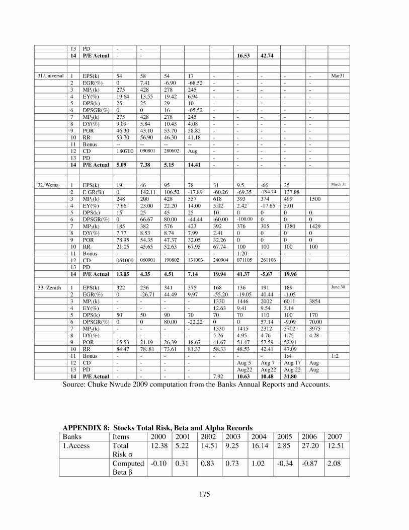
175
13 PD - - 14 P/E Actual - - 16.53 42.74 31.Universal 1 EPS(k) 54 58 54 17 - - - - - Mar31 2 EGR(%) 0 7.41 -6.90 -68.52 - - - - - 3 MP1(k) 275 428 278 245 - - - - - 4 EY(%) 19.64 13.55 19.42 6.94 - - - - - 5 DPS(k) 25 25 29 10 - - - - - 6 DPSGR(%) 0 0 16 -65.52 - - - - - 7 MP2(k) 275 428 278 245 - - - - - 8 DY(%) 9.09 5.84 10.43 4.08 - - - - - 9 POR 46.30 43.10 53.70 58.82 - - - - - 10 RR 53.70 56.90 46.30 41.18 - - - - - 11 Bonus -- -- -- -- - - - - - 12 CD 180700 090801 280602 Aug - - - - - 13 PD - - - - - 14 P/E Actual 5.09 7.38 5.15 14.41 - - - - - 32. Wema 1 EPS(k) 19 46 95 78 31 9.5 -66 25 March 31 2 E GR(%) 0 142.11 106.52 -17.89 -60.26 -69.35 -794.74 137.88 3 MP1(k) 248 200 428 557 618 393 374 499 1500 4 EY(%) 7.66 23.00 22.20 14.00 5.02 2.42 -17.65 5.01 5 DPS(k) 15 25 45 25 10 0 0 0 0 6 DPSGR(%) 0 66.67 80.00 -44.44 -60.00 -100.00 0 0 0 7 MP2(k) 185 382 576 423 392 376 305 1380 1429 8 DY(%) 7.77 8.53 8.74 7.99 2.41 0 0 0 0 9 POR 78.95 54.35 47.37 32.05 32.26 0 0 0 0 10 RR 21.05 45.65 52.63 67.95 67.74 100 100 100 100 11 Bonus - - - - - 1:20 - - - 12 CD 061000 060901 190802 131003 240904 071105 261106 - - 13 PD 14 P/E Actual 13.05 4.35 4.51 7.14 19.94 41.37 -5.67 19.96 33. Zenith 1 EPS(k) 322 236 341 375 168 136 191 189 June 30 2 EGR(%) 0 -26.71 44.49 9.97 -55.20 -19.05 40.44 -1.05 3 MP1(k) - - - - 1330 1446 2002 6011 3854 4 EY(%) - - - - 12.63 9.41 9.54 3.14 5 DPS(k) 50 50 90 70 70 70 110 100 170 6 DPSGR(%) 0 0 80.00 -22.22 0 0 57.14 -9.09 70.00 7 MP2(k) - - - - 1330 1415 2312 5702 3975 8 DY(%) - - - - 5.26 4.95 4.76 1.75 4.28 9 POR 15.53 21.19 26.39 18.67 41.67 51.47 57.59 52.91 10 RR 84.47 78..81 73.61 81.33 58.33 48.53 42.41 47.09 11 Bonus - - - - - - - 1:4 1:2 12 CD - - - - Aug 5 Aug 7 Aug 17 Aug 13 PD - - - - Aug22 Aug22 Aug 22 Aug 14 P/E Actual - - - - 7.92 10.63 10.48 31.80
Source: Chuke Nwude 2009 computation from the Banks Annual Reports and Accounts. APPENDIX 8: Stocks Total Risk, Beta and Alpha Records Banks Items 2000 2001 2002 2003 2004 2005 2006 2007 1.Access Total
Risk 12.38 5.22 14.51 9.25 16.14 2.85 27.20 12.51
Computed Beta �
-0.10 0.31 0.83 0.73 1.02 -0.34 -0.87 2.08
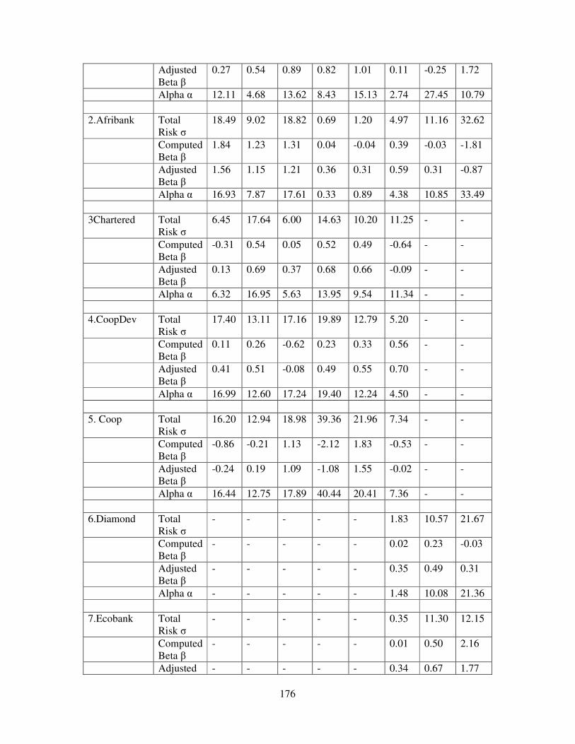
176
Adjusted Beta �
0.27 0.54 0.89 0.82 1.01 0.11 -0.25 1.72
Alpha � 12.11 4.68 13.62 8.43 15.13 2.74 27.45 10.79 2.Afribank Total
Risk 18.49 9.02 18.82 0.69 1.20 4.97 11.16 32.62
Computed Beta �
1.84 1.23 1.31 0.04 -0.04 0.39 -0.03 -1.81
Adjusted Beta �
1.56 1.15 1.21 0.36 0.31 0.59 0.31 -0.87
Alpha � 16.93 7.87 17.61 0.33 0.89 4.38 10.85 33.49 3Chartered Total
Risk 6.45 17.64 6.00 14.63 10.20 11.25 - -
Computed Beta �
-0.31 0.54 0.05 0.52 0.49 -0.64 - -
Adjusted Beta �
0.13 0.69 0.37 0.68 0.66 -0.09 - -
Alpha � 6.32 16.95 5.63 13.95 9.54 11.34 - - 4.CoopDev Total
Risk 17.40 13.11 17.16 19.89 12.79 5.20 - -
Computed Beta �
0.11 0.26 -0.62 0.23 0.33 0.56 - -
Adjusted Beta �
0.41 0.51 -0.08 0.49 0.55 0.70 - -
Alpha � 16.99 12.60 17.24 19.40 12.24 4.50 - - 5. Coop Total
Risk 16.20 12.94 18.98 39.36 21.96 7.34 - -
Computed Beta �
-0.86 -0.21 1.13 -2.12 1.83 -0.53 - -
Adjusted Beta �
-0.24 0.19 1.09 -1.08 1.55 -0.02 - -
Alpha � 16.44 12.75 17.89 40.44 20.41 7.36 - - 6.Diamond Total
Risk - - - - - 1.83 10.57 21.67
Computed Beta �
- - - - - 0.02 0.23 -0.03
Adjusted Beta �
- - - - - 0.35 0.49 0.31
Alpha � - - - - - 1.48 10.08 21.36 7.Ecobank Total
Risk - - - - - 0.35 11.30 12.15
Computed Beta �
- - - - - 0.01 0.50 2.16
Adjusted - - - - - 0.34 0.67 1.77
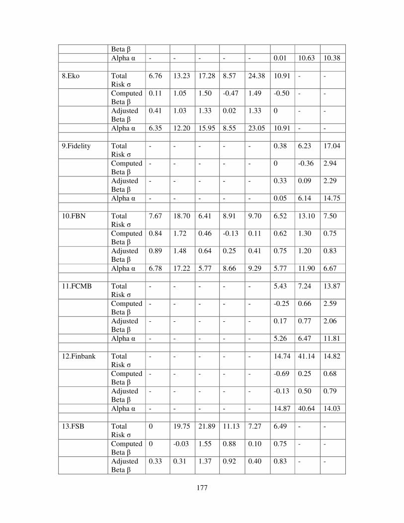
177
Beta � Alpha � - - - - - 0.01 10.63 10.38 8.Eko Total
Risk 6.76 13.23 17.28 8.57 24.38 10.91 - -
Computed Beta �
0.11 1.05 1.50 -0.47 1.49 -0.50 - -
Adjusted Beta �
0.41 1.03 1.33 0.02 1.33 0 - -
Alpha � 6.35 12.20 15.95 8.55 23.05 10.91 - - 9.Fidelity Total
Risk - - - - - 0.38 6.23 17.04
Computed Beta �
- - - - - 0 -0.36 2.94
Adjusted Beta �
- - - - - 0.33 0.09 2.29
Alpha � - - - - - 0.05 6.14 14.75 10.FBN Total
Risk 7.67 18.70 6.41 8.91 9.70 6.52 13.10 7.50
Computed Beta �
0.84 1.72 0.46 -0.13 0.11 0.62 1.30 0.75
Adjusted Beta �
0.89 1.48 0.64 0.25 0.41 0.75 1.20 0.83
Alpha � 6.78 17.22 5.77 8.66 9.29 5.77 11.90 6.67 11.FCMB Total
Risk - - - - - 5.43 7.24 13.87
Computed Beta �
- - - - - -0.25 0.66 2.59
Adjusted Beta �
- - - - - 0.17 0.77 2.06
Alpha � - - - - - 5.26 6.47 11.81 12.Finbank Total
Risk - - - - - 14.74 41.14 14.82
Computed Beta �
- - - - - -0.69 0.25 0.68
Adjusted Beta �
- - - - - -0.13 0.50 0.79
Alpha � - - - - - 14.87 40.64 14.03 13.FSB Total
Risk 0 19.75 21.89 11.13 7.27 6.49 - -
Computed Beta �
0 -0.03 1.55 0.88 0.10 0.75 - -
Adjusted Beta �
0.33 0.31 1.37 0.92 0.40 0.83 - -

178
Alpha � -0.33 19.44 20.52 10.21 6.87 5.66 - - 14.GTB Total
Risk 9.06 11.10 7.19 8.93 13.75 8.53 9.46 13.54
Computed Beta �
0.47 1.06 0.52 0.58 0.69 1.29 0.42 2.14
Adjusted Beta �
0.65 1.04 0.68 0.72 0.79 1.19 0.61 1.76
Alpha � 8.41 10.06 6.51 8.21 12.96 7.34 8.85 11.78 15.Hallmark Total
Risk 5.85 18.55 5.10 13.74 9.44 15.18 - -
Computed Beta �
-0.46 -0.13 -0.11 0.01 0.25 1.27 - -
Adjusted Beta �
0.03 0.25 0.26 0.34 0.50 1.18 - -
Alpha � 5.82 18.30 4.84 13.40 8.94 14.00 16.IBTCC Total
Risk - - - - - 2.11 7.58 17.19
Computed Beta �
- - - - - 0.18 0.04 0.43
Adjusted Beta �
- - - - - 0.45 0.36 0.62
Alpha � - - - - - 1.66 7.22 16.57 17.ICB Total
Risk - - - - - 11.93 11.94 9.31
Computed Beta �
- - - - - 0.93 1.38 1.29
Adjusted Beta �
- - - - - 0.95 1.25 1.19
Alpha � - - - - - 10.98 10.69 8.12 18.IMB Total
Risk 5.54 23.16 15.69 16.72 16.09 18.77 - -
Computed Beta �
0.03 0.92 -0.88 -0.67 1.01 2.20 - -
Adjusted Beta �
0.35 0.95 -0.25 -0.11 1.01 1.80 - -
Alpha � 5.19 22.21 15.94 16.83 15.08 16.97 - - 19.Inland Total
Risk 8.82 17.30 22.54 7.80 17.42 7.62 - -
Computed Beta �
0.26 -1.56 2.47 0.06 0.92 0.30 - -
Adjusted Beta �
0.51 -0.71 1.98 0.01 0.95 0.53 - -
Alpha � 8.31 18.01 20.56 7.79 16.47 7.09 - -
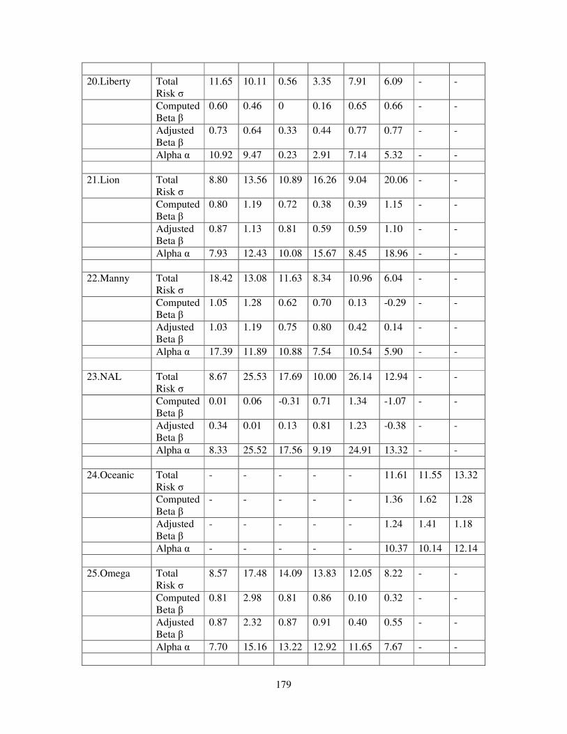
179
20.Liberty Total
Risk 11.65 10.11 0.56 3.35 7.91 6.09 - -
Computed Beta �
0.60 0.46 0 0.16 0.65 0.66 - -
Adjusted Beta �
0.73 0.64 0.33 0.44 0.77 0.77 - -
Alpha � 10.92 9.47 0.23 2.91 7.14 5.32 - - 21.Lion Total
Risk 8.80 13.56 10.89 16.26 9.04 20.06 - -
Computed Beta �
0.80 1.19 0.72 0.38 0.39 1.15 - -
Adjusted Beta �
0.87 1.13 0.81 0.59 0.59 1.10 - -
Alpha � 7.93 12.43 10.08 15.67 8.45 18.96 - - 22.Manny Total
Risk 18.42 13.08 11.63 8.34 10.96 6.04 - -
Computed Beta �
1.05 1.28 0.62 0.70 0.13 -0.29 - -
Adjusted Beta �
1.03 1.19 0.75 0.80 0.42 0.14 - -
Alpha � 17.39 11.89 10.88 7.54 10.54 5.90 - - 23.NAL Total
Risk 8.67 25.53 17.69 10.00 26.14 12.94 - -
Computed Beta �
0.01 0.06 -0.31 0.71 1.34 -1.07 - -
Adjusted Beta �
0.34 0.01 0.13 0.81 1.23 -0.38 - -
Alpha � 8.33 25.52 17.56 9.19 24.91 13.32 - - 24.Oceanic Total
Risk - - - - - 11.61 11.55 13.32
Computed Beta �
- - - - - 1.36 1.62 1.28
Adjusted Beta �
- - - - - 1.24 1.41 1.18
Alpha � - - - - - 10.37 10.14 12.14 25.Omega Total
Risk 8.57 17.48 14.09 13.83 12.05 8.22 - -
Computed Beta �
0.81 2.98 0.81 0.86 0.10 0.32 - -
Adjusted Beta �
0.87 2.32 0.87 0.91 0.40 0.55 - -
Alpha � 7.70 15.16 13.22 12.92 11.65 7.67 - -
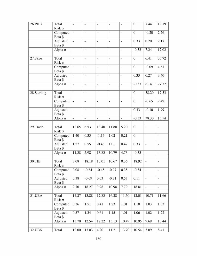
180
26.PHB Total Risk
- - - - - 0 7.44 19.19
Computed Beta �
- - - - - 0 -0.20 2.76
Adjusted Beta �
- - - - - 0.33 0.20 2.17
Alpha � - - - - - -0.33 7.24 17.02 27.Skye Total
Risk - - - - - 0 6.41 30.72
Computed Beta �
- - - - - 0 -0.09 4.61
Adjusted Beta �
- - - - - 0.33 0.27 3.40
Alpha � - - - - - -0.33 6.14 27.32 28.Sterling Total
Risk - - - - - 0 38.20 17.53
Computed Beta �
- - - - - 0 -0.65 2.49
Adjusted Beta �
- - - - - 0.33 -0.10 1.99
Alpha � - - - - - -0.33 38.30 15.54 29.Trade Total
Risk 12.65 6.53 13.40 11.80 5.20 0 - -
Computed Beta �
1.40 0.33 -1.14 1.02 0.21 0 - -
Adjusted Beta �
1.27 0.55 -0.43 1.01 0.47 0.33 - -
Alpha � 11.38 5.98 13.83 10.79 4.73 -0.33 - - 30.TIB Total
Risk 3.08 18.18 10.01 10.67 8.36 18.92 - -
Computed Beta �
0.08 -0.64 -0.45 -0.97 0.35 -0.34 - -
Adjusted Beta �
0.38 -0.09 0.03 -0.31 0.57 0.11 - -
Alpha � 2.70 18.27 9.98 10.98 7.79 18.81 - - 31.UBA Total
Risk 14.27 13.88 12.83 16.28 11.50 12.01 10.71 11.66
Computed Beta �
0.36 1.51 0.41 1.23 1.01 1.10 1.03 1.33
Adjusted Beta �
0.57 1.34 0.61 1.15 1.01 1.06 1.02 1.22
Alpha � 13.70 12.54 12.22 15.13 10.49 10.95 9.69 10.44 32.UBN Total 12.00 13.03 4.20 11.21 13.70 10.54 5.09 8.41
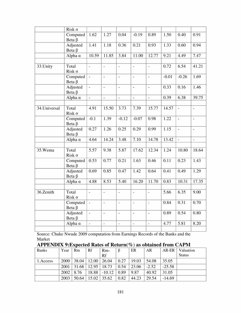
181
Risk Computed
Beta � 1.62 1.27 0.04 -0.19 0.89 1.50 0.40 0.91
Adjusted Beta �
1.41 1.18 0.36 0.21 0.93 1.33 0.60 0.94
Alpha � 10.59 11.85 3.84 11.00 12.77 9.21 4.49 7.47 33.Unity Total
Risk - - - - - 0.72 6.54 41.21
Computed Beta �
- - - - - -0.01 -0.26 1.69
Adjusted Beta �
- - - - - 0.33 0.16 1.46
Alpha � - - - - - 0.39 6.38 39.75 34.Universal Total
Risk 4.91 15.50 3.73 7.39 15.77 14.57 - -
Computed Beta �
-0.1 1.39 -0.12 -0.07 0.98 1.22 - -
Adjusted Beta �
0.27 1.26 0.25 0.29 0.99 1.15 - -
Alpha � 4.64 14.24 3.48 7.10 14.78 13.42 - - 35.Wema Total
Risk 5.57 9.38 5.87 17.62 12.34 1.24 10.80 18.64
Computed Beta �
0.53 0.77 0.21 1.63 0.46 0.11 0.23 1.43
Adjusted Beta �
0.69 0.85 0.47 1.42 0.64 0.41 0.49 1.29
Alpha � 4.88 8.53 5.40 16.20 11.70 0.83 10.31 17.35 36.Zenith Total
Risk - - - - - 5.66 6.35 9.00
Computed Beta �
- - - - - 0.84 0.31 0.70
Adjusted Beta �
- - - - - 0.89 0.54 0.80
Alpha � - - - - - 4.77 5.81 8.20 Source: Chuke Nwude 2009 computation from Earnings Records of the Banks and the Market APPENDIX 9:Expected Rates of Return(%) as obtained from CAPM Banks Year Rm Rf Rm-
Rf � ER AR AR-ER Valuation
Status 1.Access 2000 38.04 12.00 26.04 0.27 19.03 54.08 35.05 2001 31.68 12.95 18.73 0.54 23.06 -2.52 -25.58 2002 8.76 18.88 -10.12 0.89 9.87 40.92 31.05 2003 50.64 15.02 35.62 0.82 44.23 29.54 -14.69
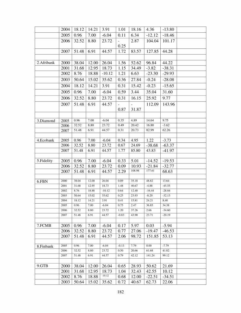
182
2004 18.12 14.21 3.91 1.01 18.16 4.36 -13.80 2005 0.96 7.00 -6.04 0.11 6.34 -12.12 -18.46 2006 32.52 8.80 23.72 -
0.25 2.87 104.04 101.17
2007 51.48 6.91 44.57 1.72 83.57 127.85 44.28 2.Afribank 2000 38.04 12.00 26.04 1.56 52.62 96.84 44.22 2001 31.68 12.95 18.73 1.15 34.49 -3.82 -38.31 2002 8.76 18.88 -10.12 1.21 6.63 -23.30 -29.93
2003 50.64 15.02 35.62 0.36 27.84 -0.24 -28.08
2004 18.12 14.21 3.91 0.31 15.42 -0.23 -15.65
2005 0.96 7.00 -6.04 0.59 3.44 35.04 31.60
2006 32.52 8.80 23.72 0.31 16.15 25.92 9.77
2007 51.48 6.91 44.57 -0.87
-31.87
112.09 143.96
3.Diamond 2005 0.96 7.00 -6.04 0.35 4.89 14.64 9.75 2006 32.52 8.80 23.72 0.49 20.42 16.80 -3.62 2007 51.48 6.91 44.57 0.31 20.73 82.99 62.26 4.Ecobank 2005 0.96 7.00 -6.04 0.34 4.95 1.22 -3.73 2006 32.52 8.80 23.72 0.67 24.69 -38.68 -63.37 2007 51.48 6.91 44.57 1.77 85.80 43.83 -41.97 5.Fidelity 2005 0.96 7.00 -6.04 0.33 5.01 -14.52 -19.53 2006 32.52 8.80 23.72 0.09 10.93 -21.84 -32.77 2007 51.48 6.91 44.57 2.29 108.98 177.61 68.63 6.FBN 2000 38.04 12.00 26.04 0.89 35.18 48.82 13.64 2001 31.68 12.95 18.73 1.48 40.67 -4.88 -45.55 2002 8.76 18.88 -10.12 0.64 12.40 -16.44 -28.84 2003 50.64 15.02 35.62 0.25 23.93 -8.20 -32.13 2004 18.12 14.21 3.91 0.41 15.81 24.21 8.40 2005 0.96 7.00 -6.04 0.75 2.47 36.85 34.38 2006 32.52 8.80 23.72 1.20 37.26 2.66 -34.60 2007 51.48 6.91 44.57 -0.83 43.90 23.71 -20.19 7.FCMB 2005 0.96 7.00 -6.04 0.17 5.97 0.03 -5.94 2006 32.52 8.80 23.72 0.77 27.06 -19.47 -46.53 2007 51.48 6.91 44.57 2.06 98.72 151.85 53.13 8.Finbank 2005 0.96 7.00 -6.04 -0.13 7.79 0.00 -7.79
2006 32.52 8.80 23.72 0.50 20.66 61.68 41.02
2007 51.48 6.91 44.57 0.79 42.12 141.24 99.12
9.GTB 2000 38.04 12.00 26.04 0.65 28.93 50.62 21.69 2001 31.68 12.95 18.73 1.04 32.43 42.55 10.12 2002 8.76 18.88 -10.12 0.68 12.00 -22.51 -34.51 2003 50.64 15.02 35.62 0.72 40.67 62.73 22.06
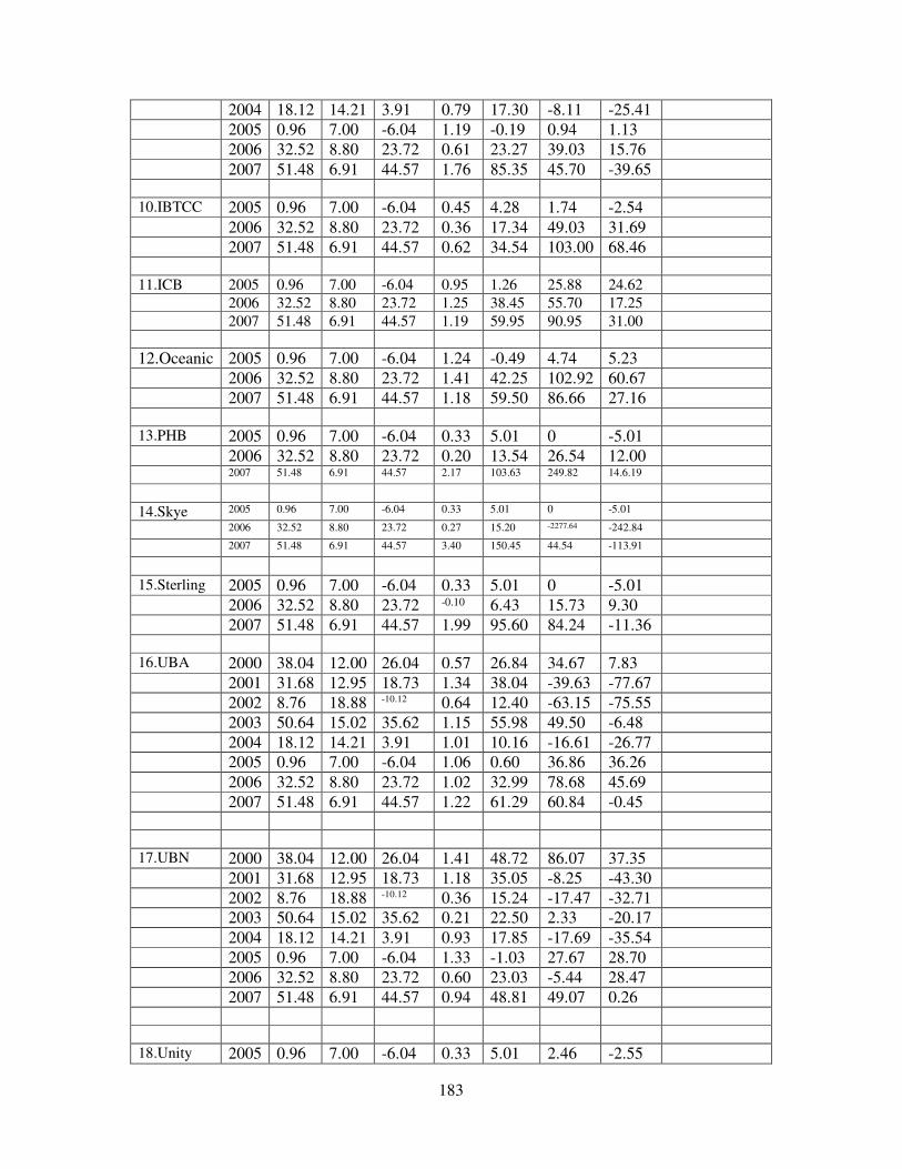
183
2004 18.12 14.21 3.91 0.79 17.30 -8.11 -25.41 2005 0.96 7.00 -6.04 1.19 -0.19 0.94 1.13 2006 32.52 8.80 23.72 0.61 23.27 39.03 15.76 2007 51.48 6.91 44.57 1.76 85.35 45.70 -39.65 10.IBTCC 2005 0.96 7.00 -6.04 0.45 4.28 1.74 -2.54 2006 32.52 8.80 23.72 0.36 17.34 49.03 31.69 2007 51.48 6.91 44.57 0.62 34.54 103.00 68.46 11.ICB 2005 0.96 7.00 -6.04 0.95 1.26 25.88 24.62 2006 32.52 8.80 23.72 1.25 38.45 55.70 17.25 2007 51.48 6.91 44.57 1.19 59.95 90.95 31.00 12.Oceanic 2005 0.96 7.00 -6.04 1.24 -0.49 4.74 5.23 2006 32.52 8.80 23.72 1.41 42.25 102.92 60.67 2007 51.48 6.91 44.57 1.18 59.50 86.66 27.16 13.PHB 2005 0.96 7.00 -6.04 0.33 5.01 0 -5.01 2006 32.52 8.80 23.72 0.20 13.54 26.54 12.00 2007 51.48 6.91 44.57 2.17 103.63 249.82 14.6.19 14.Skye 2005 0.96 7.00 -6.04 0.33 5.01 0 -5.01 2006 32.52 8.80 23.72 0.27 15.20 -2277.64 -242.84 2007 51.48 6.91 44.57 3.40 150.45 44.54 -113.91 15.Sterling 2005 0.96 7.00 -6.04 0.33 5.01 0 -5.01 2006 32.52 8.80 23.72 -0.10 6.43 15.73 9.30 2007 51.48 6.91 44.57 1.99 95.60 84.24 -11.36 16.UBA 2000 38.04 12.00 26.04 0.57 26.84 34.67 7.83 2001 31.68 12.95 18.73 1.34 38.04 -39.63 -77.67 2002 8.76 18.88 -10.12 0.64 12.40 -63.15 -75.55 2003 50.64 15.02 35.62 1.15 55.98 49.50 -6.48 2004 18.12 14.21 3.91 1.01 10.16 -16.61 -26.77 2005 0.96 7.00 -6.04 1.06 0.60 36.86 36.26 2006 32.52 8.80 23.72 1.02 32.99 78.68 45.69 2007 51.48 6.91 44.57 1.22 61.29 60.84 -0.45 17.UBN 2000 38.04 12.00 26.04 1.41 48.72 86.07 37.35 2001 31.68 12.95 18.73 1.18 35.05 -8.25 -43.30 2002 8.76 18.88 -10.12 0.36 15.24 -17.47 -32.71 2003 50.64 15.02 35.62 0.21 22.50 2.33 -20.17 2004 18.12 14.21 3.91 0.93 17.85 -17.69 -35.54 2005 0.96 7.00 -6.04 1.33 -1.03 27.67 28.70 2006 32.52 8.80 23.72 0.60 23.03 -5.44 28.47 2007 51.48 6.91 44.57 0.94 48.81 49.07 0.26 18.Unity 2005 0.96 7.00 -6.04 0.33 5.01 2.46 -2.55
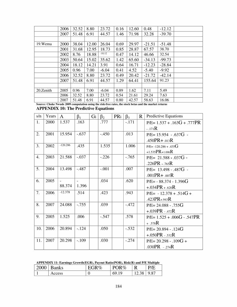
184
2006 32.52 8.80 23.72 0.16 12.60 0.48 -12.12 2007 51.48 6.91 44.57 1.46 71.98 32.28 -39.70 19.Wema 2000 38.04 12.00 26.04 0.69 29.97 -21.51 -51.48 2001 31.68 12.95 18.73 0.85 28.87 67.57 38.70 2002 8.76 18.88 -10.12 0.47 14.12 46.66 32.54 2003 50.64 15.02 35.62 1.42 65.60 -34.13 -99.73 2004 18.12 14.21 3.91 0.64 16.71 -12.23 -28.84 2005 0.96 7.00 -6.04 0.41 4.52 -5.40 -9.92 2006 32.52 8.80 23.72 0.49 20.42 -21.72 -42.14 2007 51.48 6.91 44.57 1.29 64.41 155.64 91.23 20.Zenith 2005 0.96 7.00 -6.04 0.89 1.62 7.11 5.49 2006 32.52 8.80 23.72 0.54 21.61 29.24 7.63 2007 51.48 6.91 44.57 0.80 42.57 58.63 16.06 Source: Chuke Nwude 2009 computation using the risk-free rates, the stock betas and the market returns APPENDIX 10: The Predictive Equations
s/n Years �1 Gi �2 PRi �3 R Predictive Equations 1. 2000 1.537 .163 .777 -.171 P/E= 1.537 + .163G + .777PR
- .171R 2. 2001 15.954 -.637 -.450 .013 P/E= 15.954 - .637G -
.450PR+ .013R 3. 2002 -120.286 .435 1.535 1.006 P/E= -120.286 + .435G
+1.535PR+1.006R 4. 2003 21.588 -.037 -.226 -.765 P/E= 21.588 - .037G -
.226PR - .765R 5. 2004 13.498 -.487 -.001 .007 P/E= 13.498 - .487G -
.001PR+ .007R 6. 2005 -
88.374 -1.396
.034 .620 P/E= - 88.374 - 1.396G +.034PR + .620R
7. 2006 -12.378 .514 .423 .943 P/E= - 12.378 + .514G + .423PR+.943R
8. 2007 24.088 -.755 .039 -.472 P/E= 24.088 - .755G +.039PR - .472R
9. 2005 1.525 .006 -.547 .578 P/E= 1.525 + .006G - .547PR + .578R
10. 2006 20.894 -.124 .050 -.532 P/E= 20.894 - .124G +.050PR - .532R
11. 2007 20.298 -.109 .030 -.274 P/E= 20.298 - .109G + .030PR - .274R
APPENDIX 11: Earnings Growth(EGR), Payout Ratio(POR), Risk(R) and P/E Multiple
2000 Banks EGR% POR% R P/E 1 Access 0 69.19 12.38 9.87
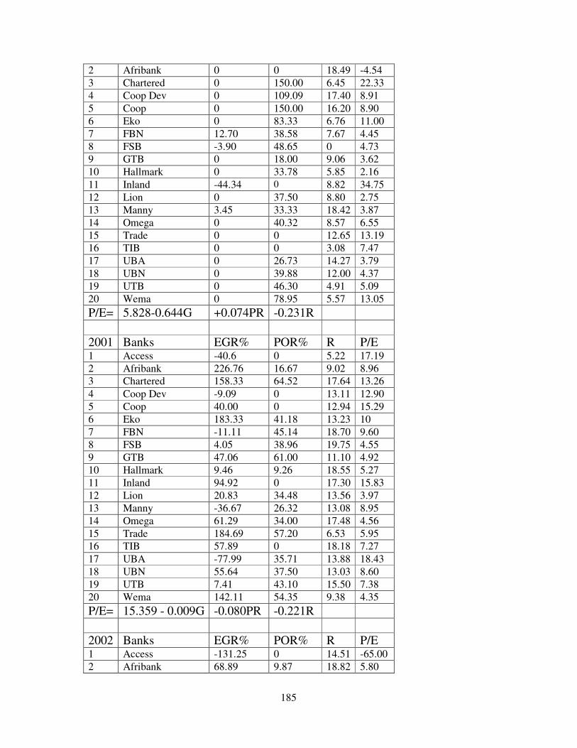
185
2 Afribank 0 0 18.49 -4.54 3 Chartered 0 150.00 6.45 22.33 4 Coop Dev 0 109.09 17.40 8.91 5 Coop 0 150.00 16.20 8.90 6 Eko 0 83.33 6.76 11.00 7 FBN 12.70 38.58 7.67 4.45 8 FSB -3.90 48.65 0 4.73 9 GTB 0 18.00 9.06 3.62 10 Hallmark 0 33.78 5.85 2.16 11 Inland -44.34 0 8.82 34.75 12 Lion 0 37.50 8.80 2.75 13 Manny 3.45 33.33 18.42 3.87 14 Omega 0 40.32 8.57 6.55 15 Trade 0 0 12.65 13.19 16 TIB 0 0 3.08 7.47 17 UBA 0 26.73 14.27 3.79 18 UBN 0 39.88 12.00 4.37 19 UTB 0 46.30 4.91 5.09 20 Wema 0 78.95 5.57 13.05 P/E= 5.828-0.644G +0.074PR -0.231R 2001 Banks EGR% POR% R P/E 1 Access -40.6 0 5.22 17.19 2 Afribank 226.76 16.67 9.02 8.96 3 Chartered 158.33 64.52 17.64 13.26 4 Coop Dev -9.09 0 13.11 12.90 5 Coop 40.00 0 12.94 15.29 6 Eko 183.33 41.18 13.23 10 7 FBN -11.11 45.14 18.70 9.60 8 FSB 4.05 38.96 19.75 4.55 9 GTB 47.06 61.00 11.10 4.92 10 Hallmark 9.46 9.26 18.55 5.27 11 Inland 94.92 0 17.30 15.83 12 Lion 20.83 34.48 13.56 3.97 13 Manny -36.67 26.32 13.08 8.95 14 Omega 61.29 34.00 17.48 4.56 15 Trade 184.69 57.20 6.53 5.95 16 TIB 57.89 0 18.18 7.27 17 UBA -77.99 35.71 13.88 18.43 18 UBN 55.64 37.50 13.03 8.60 19 UTB 7.41 43.10 15.50 7.38 20 Wema 142.11 54.35 9.38 4.35 P/E= 15.359 - 0.009G -0.080PR -0.221R 2002 Banks EGR% POR% R P/E 1 Access -131.25 0 14.51 -65.00 2 Afribank 68.89 9.87 18.82 5.80
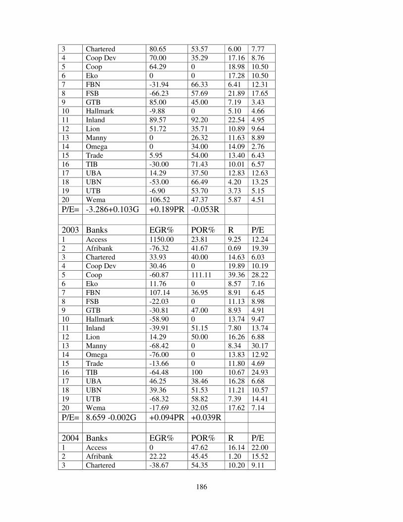
186
3 Chartered 80.65 53.57 6.00 7.77 4 Coop Dev 70.00 35.29 17.16 8.76 5 Coop 64.29 0 18.98 10.50 6 Eko 0 0 17.28 10.50 7 FBN -31.94 66.33 6.41 12.31 8 FSB -66.23 57.69 21.89 17.65 9 GTB 85.00 45.00 7.19 3.43 10 Hallmark -9.88 0 5.10 4.66 11 Inland 89.57 92.20 22.54 4.95 12 Lion 51.72 35.71 10.89 9.64 13 Manny 0 26.32 11.63 8.89 14 Omega 0 34.00 14.09 2.76 15 Trade 5.95 54.00 13.40 6.43 16 TIB -30.00 71.43 10.01 6.57 17 UBA 14.29 37.50 12.83 12.63 18 UBN -53.00 66.49 4.20 13.25 19 UTB -6.90 53.70 3.73 5.15 20 Wema 106.52 47.37 5.87 4.51 P/E= -3.286+0.103G +0.189PR -0.053R 2003 Banks EGR% POR% R P/E 1 Access 1150.00 23.81 9.25 12.24 2 Afribank -76.32 41.67 0.69 19.39 3 Chartered 33.93 40.00 14.63 6.03 4 Coop Dev 30.46 0 19.89 10.19 5 Coop -60.87 111.11 39.36 28.22 6 Eko 11.76 0 8.57 7.16 7 FBN 107.14 36.95 8.91 6.45 8 FSB -22.03 0 11.13 8.98 9 GTB -30.81 47.00 8.93 4.91 10 Hallmark -58.90 0 13.74 9.47 11 Inland -39.91 51.15 7.80 13.74 12 Lion 14.29 50.00 16.26 6.88 13 Manny -68.42 0 8.34 30.17 14 Omega -76.00 0 13.83 12.92 15 Trade -13.66 0 11.80 4.69 16 TIB -64.48 100 10.67 24.93 17 UBA 46.25 38.46 16.28 6.68 18 UBN 39.36 51.53 11.21 10.57 19 UTB -68.32 58.82 7.39 14.41 20 Wema -17.69 32.05 17.62 7.14 P/E= 8.659 -0.002G +0.094PR +0.039R 2004 Banks EGR% POR% R P/E 1 Access 0 47.62 16.14 22.00 2 Afribank 22.22 45.45 1.20 15.52 3 Chartered -38.67 54.35 10.20 9.11
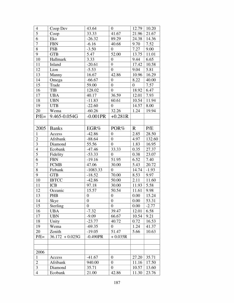
187
4 Coop Dev 43.64 0 12.79 10.20 5 Coop 33.33 41.67 21.96 21.67 6 Eko -26.32 89.29 24.38 14.36 7 FBN -6.16 40.68 9.70 7.52 8 FSB -3.50 0 7.27 9.00 9 GTB 5.47 52.00 13.75 11.01 10 Hallmark 3.33 0 9.44 6.65 11 Inland -20.61 0 17.42 10.58 12 Lion -5.53 0 9.04 5.81 13 Manny 16.67 42.86 10.96 16.29 14 Omega -66.67 0 8.22 40.00 15 Trade 59.00 0 0 7.57 16 TIB 128.02 0 18.92 6.47 17 UBA 40.17 36.59 12.01 7.93 18 UBN -11.83 60.61 10.54 11.94 19 UTB -22.60 0 14.57 8.00 20 Wema -60.26 32.26 1.24 19.94 P/E= 9.465-0.054G -0.001PR +0.281R 2005 Banks EGR% POR% R P/E 1 Access -42.86 0 2.85 28.50 2 Afribank -88.64 0 4.97 132.60 3 Diamond 55.56 0 1.83 16.95 4 Ecobank -47.46 33.33 0.35 27.37 5 Fidelity -53.33 0 0.38 23.07 6 FBN -19.16 51.95 6.52 7.40 7 FCMB 47.06 30.00 5.43 20.72 8 Firbank -1083.33 0 14.74 -1.93 9 GTB -18.52 70.00 8.53 9.97 10 IBTCC -42.86 50.00 2.11 11.60 11 ICB 97.18 30.00 11.93 5.58 12 Oceanic 15.57 50.54 11.61 9.98 13 PHB 0 0 0.00 15.24 14 Skye 0 0 0.00 53.31 15 Sterling 0 0 0.00 -2.77 16 UBA -7.32 39.47 12.01 6.58 17 UBN -9.09 66.67 10.54 9.21 18 Unity -23.77 40.72 0.72 16.53 19 Wema -69.35 0 1.24 41.37 20 Zenith -19.05 51.47 5.66 10.63 P/E= 36.172 + 0.025G -0.490PR + 0.035R 2006 1 Access -41.67 0 27.20 35.71 2 Afribank 940.00 0 11.16 17.50 3 Diamond 35.71 0 10.57 13.60 4 Ecobank 21.00 42.86 11.30 23.76
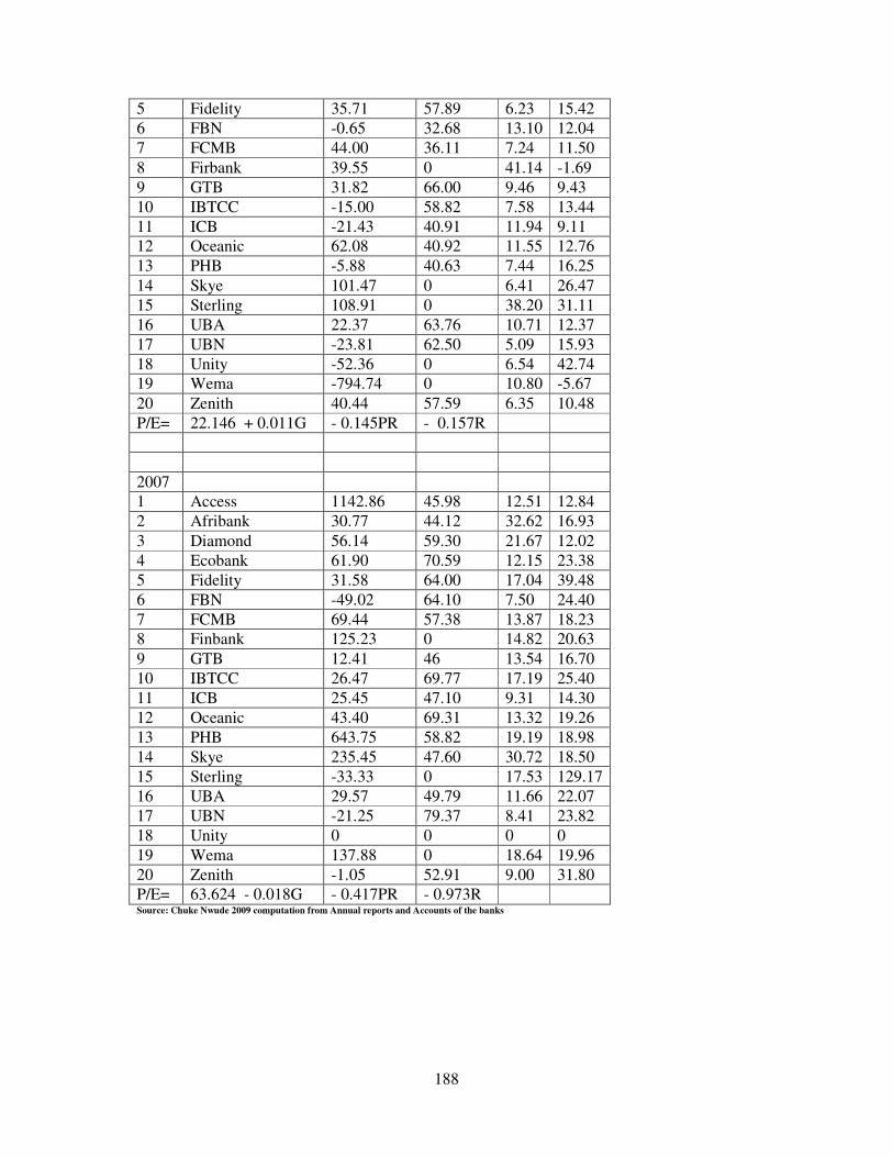
188
5 Fidelity 35.71 57.89 6.23 15.42 6 FBN -0.65 32.68 13.10 12.04 7 FCMB 44.00 36.11 7.24 11.50 8 Firbank 39.55 0 41.14 -1.69 9 GTB 31.82 66.00 9.46 9.43 10 IBTCC -15.00 58.82 7.58 13.44 11 ICB -21.43 40.91 11.94 9.11 12 Oceanic 62.08 40.92 11.55 12.76 13 PHB -5.88 40.63 7.44 16.25 14 Skye 101.47 0 6.41 26.47 15 Sterling 108.91 0 38.20 31.11 16 UBA 22.37 63.76 10.71 12.37 17 UBN -23.81 62.50 5.09 15.93 18 Unity -52.36 0 6.54 42.74 19 Wema -794.74 0 10.80 -5.67 20 Zenith 40.44 57.59 6.35 10.48 P/E= 22.146 + 0.011G - 0.145PR - 0.157R 2007 1 Access 1142.86 45.98 12.51 12.84 2 Afribank 30.77 44.12 32.62 16.93 3 Diamond 56.14 59.30 21.67 12.02 4 Ecobank 61.90 70.59 12.15 23.38 5 Fidelity 31.58 64.00 17.04 39.48 6 FBN -49.02 64.10 7.50 24.40 7 FCMB 69.44 57.38 13.87 18.23 8 Finbank 125.23 0 14.82 20.63 9 GTB 12.41 46 13.54 16.70 10 IBTCC 26.47 69.77 17.19 25.40 11 ICB 25.45 47.10 9.31 14.30 12 Oceanic 43.40 69.31 13.32 19.26 13 PHB 643.75 58.82 19.19 18.98 14 Skye 235.45 47.60 30.72 18.50 15 Sterling -33.33 0 17.53 129.17 16 UBA 29.57 49.79 11.66 22.07 17 UBN -21.25 79.37 8.41 23.82 18 Unity 0 0 0 0 19 Wema 137.88 0 18.64 19.96 20 Zenith -1.05 52.91 9.00 31.80 P/E= 63.624 - 0.018G - 0.417PR - 0.973R Source: Chuke Nwude 2009 computation from Annual reports and Accounts of the banks
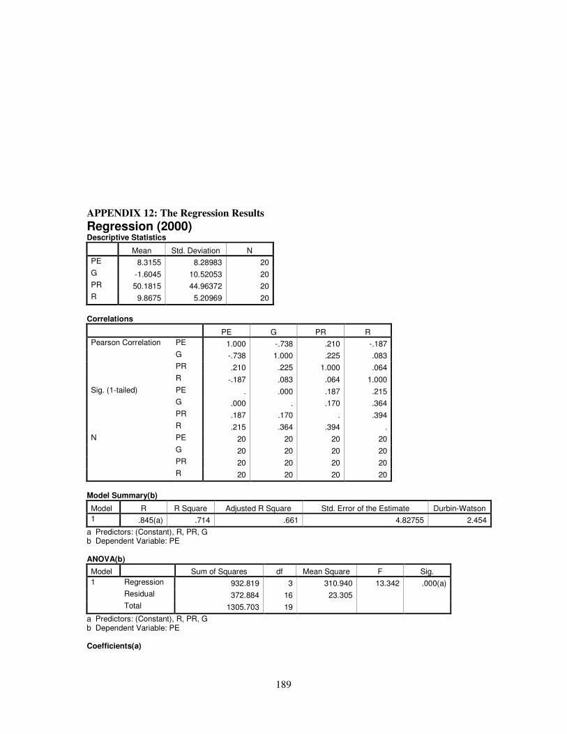
189
APPENDIX 12: The Regression Results Regression (2000) Descriptive Statistics
Mean Std. Deviation N PE 8.3155 8.28983 20 G -1.6045 10.52053 20 PR 50.1815 44.96372 20 R 9.8675 5.20969 20
Correlations
PE G PR R Pearson Correlation PE 1.000 -.738 .210 -.187 G -.738 1.000 .225 .083 PR .210 .225 1.000 .064 R -.187 .083 .064 1.000 Sig. (1-tailed) PE . .000 .187 .215 G .000 . .170 .364 PR .187 .170 . .394 R .215 .364 .394 . N PE 20 20 20 20 G 20 20 20 20 PR 20 20 20 20 R 20 20 20 20
Model Summary(b)
Model R R Square Adjusted R Square Std. Error of the Estimate Durbin-Watson 1 .845(a) .714 .661 4.82755 2.454
a Predictors: (Constant), R, PR, G b Dependent Variable: PE ANOVA(b)
Model Sum of Squares df Mean Square F Sig. 1 Regression 932.819 3 310.940 13.342 .000(a) Residual 372.884 16 23.305 Total 1305.703 19
a Predictors: (Constant), R, PR, G b Dependent Variable: PE Coefficients(a)
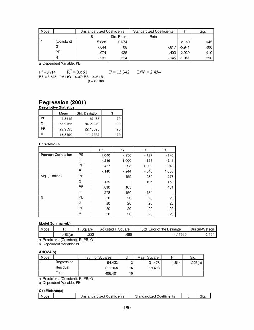
190
Model Unstandardized Coefficients Standardized Coefficients T Sig. B Std. Error Beta 1 (Constant) 5.828 2.674 2.180 .045 G -.644 .108 -.817 -5.941 .000 PR .074 .025 .403 2.939 .010 R -.231 .214 -.145 -1.081 .296
a Dependent Variable: PE R2 = 0.714 �2 = 0.661 F = 13.342 DW = 2.454 PE = 5.828 - 0.644G + 0.074PR - 0.231R (t = 2.180)
Regression (2001) Descriptive Statistics
Mean Std. Deviation N PE 9.3615 4.62488 20 G 55.9155 84.22319 20 PR 29.9695 22.16895 20 R 13.8590 4.12552 20
Correlations
PE G PR R Pearson Correlation PE 1.000 -.236 -.427 -.140 G -.236 1.000 .293 -.244 PR -.427 .293 1.000 -.040 R -.140 -.244 -.040 1.000 Sig. (1-tailed) PE . .159 .030 .278 G .159 . .105 .150 PR .030 .105 . .434 R .278 .150 .434 . N PE 20 20 20 20 G 20 20 20 20 PR 20 20 20 20 R 20 20 20 20
Model Summary(b)
Model R R Square Adjusted R Square Std. Error of the Estimate Durbin-Watson 1 .482(a) .232 .088 4.41565 2.154
a Predictors: (Constant), R, PR, G b Dependent Variable: PE ANOVA(b) Model Sum of Squares df Mean Square F Sig. 1 Regression 94.433 3 31.478 1.614 .225(a) Residual 311.968 16 19.498 Total 406.401 19
a Predictors: (Constant), R, PR, G b Dependent Variable: PE Coefficients(a)
Model Unstandardized Coefficients Standardized Coefficients t Sig.
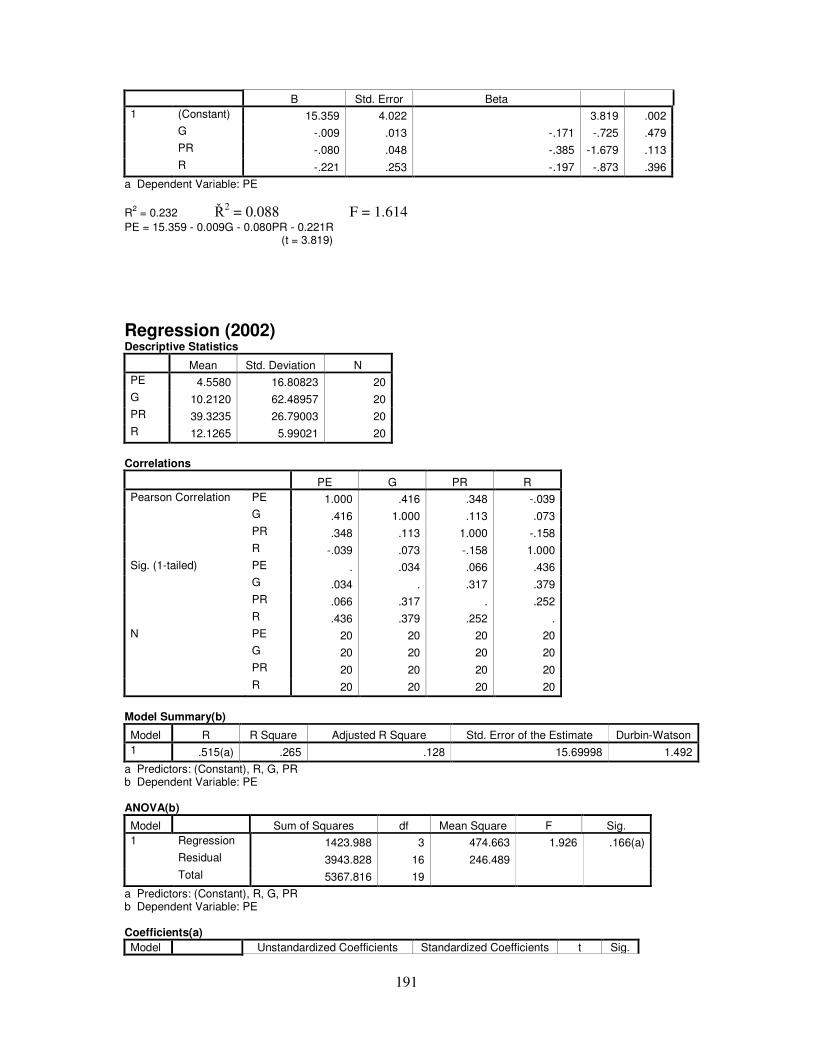
191
B Std. Error Beta 1 (Constant) 15.359 4.022 3.819 .002 G -.009 .013 -.171 -.725 .479 PR -.080 .048 -.385 -1.679 .113 R -.221 .253 -.197 -.873 .396
a Dependent Variable: PE R2 = 0.232 �2 = 0.088 F = 1.614 PE = 15.359 - 0.009G - 0.080PR - 0.221R (t = 3.819)
Regression (2002) Descriptive Statistics
Mean Std. Deviation N PE 4.5580 16.80823 20 G 10.2120 62.48957 20 PR 39.3235 26.79003 20 R 12.1265 5.99021 20
Correlations
PE G PR R Pearson Correlation PE 1.000 .416 .348 -.039 G .416 1.000 .113 .073 PR .348 .113 1.000 -.158 R -.039 .073 -.158 1.000 Sig. (1-tailed) PE . .034 .066 .436 G .034 . .317 .379 PR .066 .317 . .252 R .436 .379 .252 . N PE 20 20 20 20 G 20 20 20 20 PR 20 20 20 20 R 20 20 20 20
Model Summary(b)
Model R R Square Adjusted R Square Std. Error of the Estimate Durbin-Watson 1 .515(a) .265 .128 15.69998 1.492
a Predictors: (Constant), R, G, PR b Dependent Variable: PE ANOVA(b)
Model Sum of Squares df Mean Square F Sig. 1 Regression 1423.988 3 474.663 1.926 .166(a) Residual 3943.828 16 246.489 Total 5367.816 19
a Predictors: (Constant), R, G, PR b Dependent Variable: PE Coefficients(a) Model Unstandardized Coefficients Standardized Coefficients t Sig.
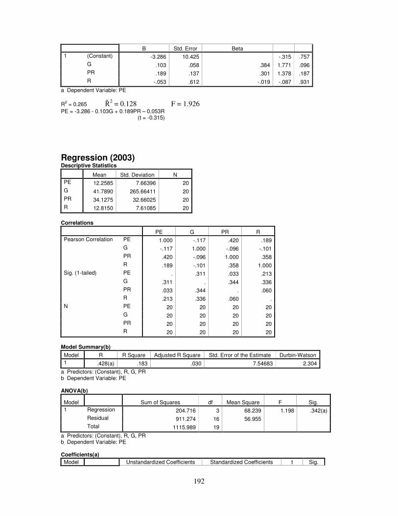
192
B Std. Error Beta 1 (Constant) -3.286 10.425 -.315 .757 G .103 .058 .384 1.771 .096 PR .189 .137 .301 1.378 .187 R -.053 .612 -.019 -.087 .931
a Dependent Variable: PE R2 = 0.265 �2 = 0.128 F = 1.926 PE = -3.286 - 0.103G + 0.189PR – 0.053R (t = -0.315)
Regression (2003) Descriptive Statistics
Mean Std. Deviation N PE 12.2585 7.66396 20 G 41.7890 265.66411 20 PR 34.1275 32.66025 20 R 12.8150 7.61085 20
Correlations
PE G PR R Pearson Correlation PE 1.000 -.117 .420 .189 G -.117 1.000 -.096 -.101 PR .420 -.096 1.000 .358 R .189 -.101 .358 1.000 Sig. (1-tailed) PE . .311 .033 .213 G .311 . .344 .336 PR .033 .344 . .060 R .213 .336 .060 . N PE 20 20 20 20 G 20 20 20 20 PR 20 20 20 20 R 20 20 20 20
Model Summary(b) Model R R Square Adjusted R Square Std. Error of the Estimate Durbin-Watson 1 .428(a) .183 .030 7.54683 2.304
a Predictors: (Constant), R, G, PR b Dependent Variable: PE ANOVA(b)
Model Sum of Squares df Mean Square F Sig. 1 Regression 204.716 3 68.239 1.198 .342(a) Residual 911.274 16 56.955 Total 1115.989 19
a Predictors: (Constant), R, G, PR b Dependent Variable: PE Coefficients(a) Model Unstandardized Coefficients Standardized Coefficients t Sig.
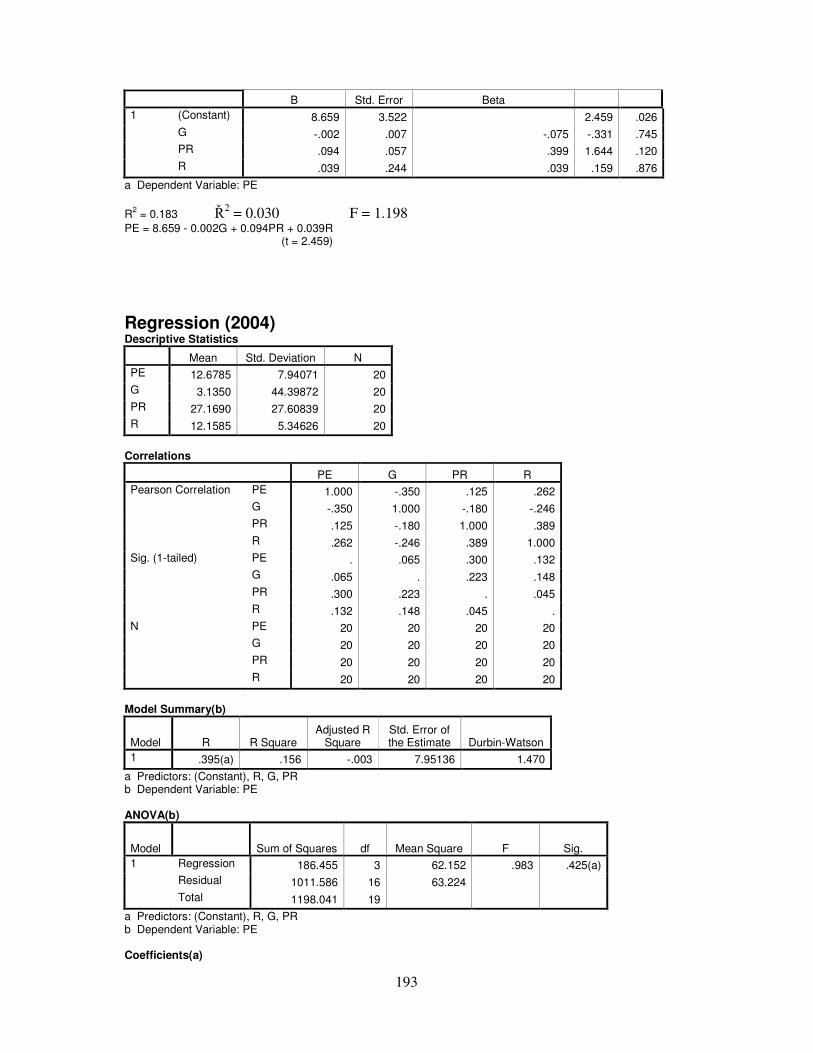
193
B Std. Error Beta 1 (Constant) 8.659 3.522 2.459 .026 G -.002 .007 -.075 -.331 .745 PR .094 .057 .399 1.644 .120 R .039 .244 .039 .159 .876
a Dependent Variable: PE R2 = 0.183 �2 = 0.030 F = 1.198 PE = 8.659 - 0.002G + 0.094PR + 0.039R (t = 2.459)
Regression (2004) Descriptive Statistics
Mean Std. Deviation N PE 12.6785 7.94071 20 G 3.1350 44.39872 20 PR 27.1690 27.60839 20 R 12.1585 5.34626 20
Correlations
PE G PR R Pearson Correlation PE 1.000 -.350 .125 .262 G -.350 1.000 -.180 -.246 PR .125 -.180 1.000 .389 R .262 -.246 .389 1.000 Sig. (1-tailed) PE . .065 .300 .132 G .065 . .223 .148 PR .300 .223 . .045 R .132 .148 .045 . N PE 20 20 20 20 G 20 20 20 20 PR 20 20 20 20 R 20 20 20 20
Model Summary(b)
Model R R Square Adjusted R
Square Std. Error of the Estimate Durbin-Watson
1 .395(a) .156 -.003 7.95136 1.470 a Predictors: (Constant), R, G, PR b Dependent Variable: PE ANOVA(b)
Model Sum of Squares df Mean Square F Sig. 1 Regression 186.455 3 62.152 .983 .425(a) Residual 1011.586 16 63.224 Total 1198.041 19
a Predictors: (Constant), R, G, PR b Dependent Variable: PE Coefficients(a)
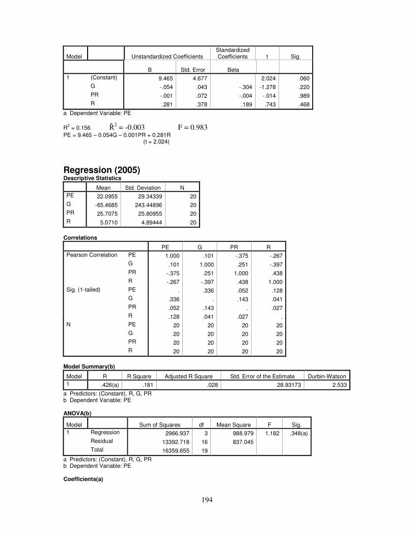
194
Model Unstandardized Coefficients Standardized Coefficients t Sig.
B Std. Error Beta 1 (Constant) 9.465 4.677 2.024 .060 G -.054 .043 -.304 -1.278 .220 PR -.001 .072 -.004 -.014 .989 R .281 .378 .189 .743 .468
a Dependent Variable: PE R2 = 0.156 �2 = -0.003 F = 0.983 PE = 9.465 – 0.054G – 0.001PR + 0.281R (t = 2.024)
Regression (2005) Descriptive Statistics
Mean Std. Deviation N PE 22.0955 29.34339 20 G -65.4685 243.44896 20 PR 25.7075 25.80955 20 R 5.0710 4.89444 20
Correlations
PE G PR R Pearson Correlation PE 1.000 .101 -.375 -.267 G .101 1.000 .251 -.397 PR -.375 .251 1.000 .438 R -.267 -.397 .438 1.000 Sig. (1-tailed) PE . .336 .052 .128 G .336 . .143 .041 PR .052 .143 . .027 R .128 .041 .027 . N PE 20 20 20 20 G 20 20 20 20 PR 20 20 20 20 R 20 20 20 20
Model Summary(b)
Model R R Square Adjusted R Square Std. Error of the Estimate Durbin-Watson 1 .426(a) .181 .028 28.93173 2.533
a Predictors: (Constant), R, G, PR b Dependent Variable: PE ANOVA(b)
Model Sum of Squares df Mean Square F Sig. 1 Regression 2966.937 3 988.979 1.182 .348(a) Residual 13392.718 16 837.045 Total 16359.655 19
a Predictors: (Constant), R, G, PR b Dependent Variable: PE Coefficients(a)
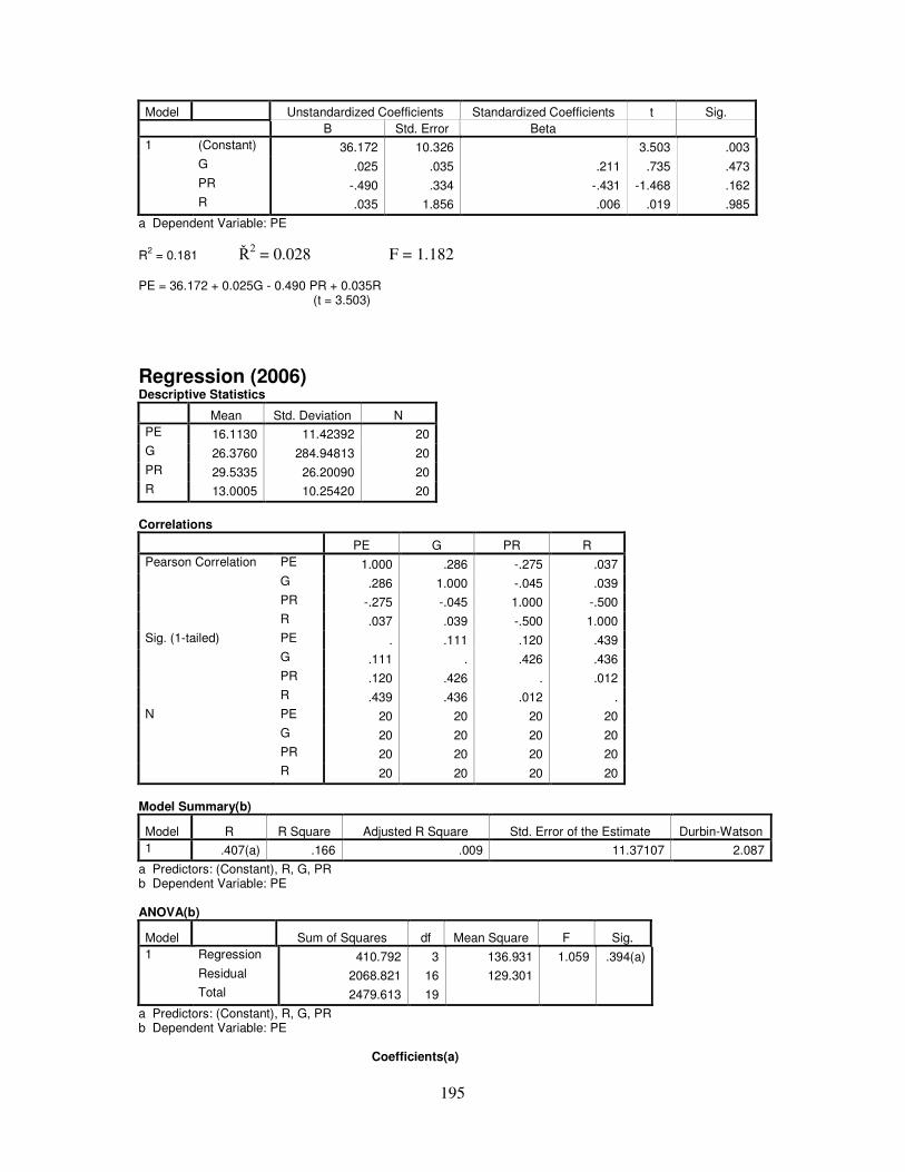
195
Model Unstandardized Coefficients Standardized Coefficients t Sig. B Std. Error Beta 1 (Constant) 36.172 10.326 3.503 .003 G .025 .035 .211 .735 .473 PR -.490 .334 -.431 -1.468 .162 R .035 1.856 .006 .019 .985
a Dependent Variable: PE R2 = 0.181 �2 = 0.028 F = 1.182 PE = 36.172 + 0.025G - 0.490 PR + 0.035R (t = 3.503)
Regression (2006) Descriptive Statistics
Mean Std. Deviation N PE 16.1130 11.42392 20 G 26.3760 284.94813 20 PR 29.5335 26.20090 20 R 13.0005 10.25420 20
Correlations
PE G PR R Pearson Correlation PE 1.000 .286 -.275 .037 G .286 1.000 -.045 .039 PR -.275 -.045 1.000 -.500 R .037 .039 -.500 1.000 Sig. (1-tailed) PE . .111 .120 .439 G .111 . .426 .436 PR .120 .426 . .012 R .439 .436 .012 . N PE 20 20 20 20 G 20 20 20 20 PR 20 20 20 20 R 20 20 20 20
Model Summary(b)
Model R R Square Adjusted R Square Std. Error of the Estimate Durbin-Watson 1 .407(a) .166 .009 11.37107 2.087
a Predictors: (Constant), R, G, PR b Dependent Variable: PE ANOVA(b)
Model Sum of Squares df Mean Square F Sig. 1 Regression 410.792 3 136.931 1.059 .394(a) Residual 2068.821 16 129.301 Total 2479.613 19
a Predictors: (Constant), R, G, PR b Dependent Variable: PE Coefficients(a)
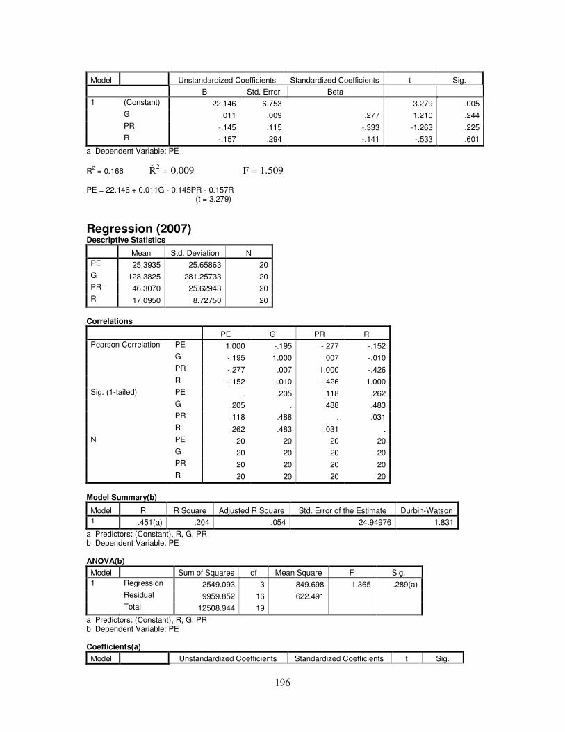
196
Model Unstandardized Coefficients Standardized Coefficients t Sig. B Std. Error Beta 1 (Constant) 22.146 6.753 3.279 .005 G .011 .009 .277 1.210 .244 PR -.145 .115 -.333 -1.263 .225 R -.157 .294 -.141 -.533 .601
a Dependent Variable: PE R2 = 0.166 �2 = 0.009 F = 1.509 PE = 22.146 + 0.011G - 0.145PR - 0.157R (t = 3.279)
Regression (2007) Descriptive Statistics
Mean Std. Deviation N PE 25.3935 25.65863 20 G 128.3825 281.25733 20 PR 46.3070 25.62943 20 R 17.0950 8.72750 20
Correlations
PE G PR R Pearson Correlation PE 1.000 -.195 -.277 -.152 G -.195 1.000 .007 -.010 PR -.277 .007 1.000 -.426 R -.152 -.010 -.426 1.000 Sig. (1-tailed) PE . .205 .118 .262 G .205 . .488 .483 PR .118 .488 . .031 R .262 .483 .031 . N PE 20 20 20 20 G 20 20 20 20 PR 20 20 20 20 R 20 20 20 20
Model Summary(b)
Model R R Square Adjusted R Square Std. Error of the Estimate Durbin-Watson 1 .451(a) .204 .054 24.94976 1.831
a Predictors: (Constant), R, G, PR b Dependent Variable: PE ANOVA(b) Model Sum of Squares df Mean Square F Sig. 1 Regression 2549.093 3 849.698 1.365 .289(a) Residual 9959.852 16 622.491 Total 12508.944 19
a Predictors: (Constant), R, G, PR b Dependent Variable: PE Coefficients(a) Model Unstandardized Coefficients Standardized Coefficients t Sig.
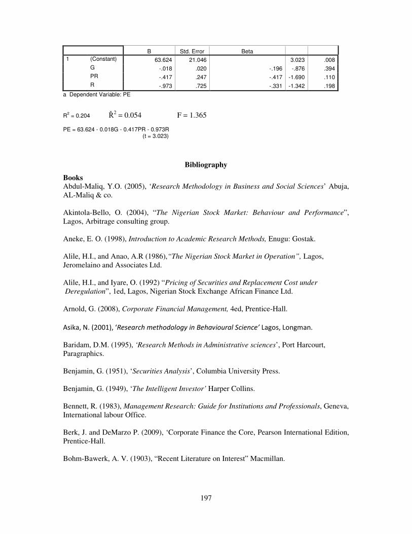
197
B Std. Error Beta 1 (Constant) 63.624 21.046 3.023 .008 G -.018 .020 -.196 -.876 .394 PR -.417 .247 -.417 -1.690 .110 R -.973 .725 -.331 -1.342 .198
a Dependent Variable: PE R2 = 0.204 �2 = 0.054 F = 1.365 PE = 63.624 - 0.018G - 0.417PR - 0.973R (t = 3.023)
Bibliography
Books Abdul-Maliq, Y.O. (2005), ‘Research Methodology in Business and Social Sciences’ Abuja, AL-Maliq & co. Akintola-Bello, O. (2004), “The Nigerian Stock Market: Behaviour and Performance”, Lagos, Arbitrage consulting group. Aneke, E. O. (1998), Introduction to Academic Research Methods, Enugu: Gostak. Alile, H.I., and Anao, A.R (1986),“The Nigerian Stock Market in Operation”, Lagos, Jeromelaino and Associates Ltd. Alile, H.I., and Iyare, O. (1992) “Pricing of Securities and Replacement Cost under Deregulation”, 1ed, Lagos, Nigerian Stock Exchange African Finance Ltd. Arnold, G. (2008), Corporate Financial Management, 4ed, Prentice-Hall. �
��� ���� ������������������������� ����������������� ���������������������� ����������������������������� Baridam, D.M. (1995), ‘Research Methods in Administrative sciences’, Port Harcourt, Paragraphics. Benjamin, G. (1951), ‘Securities Analysis’, Columbia University Press. Benjamin, G. (1949), ‘The Intelligent Investor’ Harper Collins. Bennett, R. (1983), Management Research: Guide for Institutions and Professionals, Geneva, International labour Office. Berk, J. and DeMarzo P. (2009), ‘Corporate Finance the Core, Pearson International Edition, Prentice-Hall. Bohm-Bawerk, A. V. (1903), “Recent Literature on Interest” Macmillan.

198
Brealey, R. A. and Myers, S. E. (2003), ‘Principles of Corporate Finance’, 7ed, Irwin, McGraw-Hill. Brealery, A. (2004), ‘Investment Valuation’, 3ed, New York, John Wiley. �
Cohen, J.B.; Zinbrag, E. D. and Zeikel, A. (1977), “Investment Analysis and Portfolio Management”, Homewood, III R.D. Irwin. ����������������������������������������������������������������������
Copeland, T. E.; Koller, T. and Murrin, J. (1990), ‘Valuation: Measuring and Managing the Value of companies’ John Wiley and Son.������������� Curran,W. S.(1970),“Principle of Financial Management”New York, McGraw Hill. Damodaran, A. (2006), ‘Damodaran on valuation’, 2ed, John Wiley & Sons. Damodaran, A. (2002), ‘Investment Valuation Tools and Techniques for Determining Value” New York, John Wiley and Sons. Damodaran, A. (2001), ‘Corporate Finance: Theory and Practice, 2ed, New York, John Wiley and sons. Die-bold, B. V. (1962), Understanding Educational Research New York: McGraw-Hill. Dodd, D. and Benjamin, G. (1934), ‘Security Analysis’ New York, McGraw Hill. Edwards, E. and Bell, P. (1961), ‘The theory and management of Business Income, Berkley, University of California press.
Ezejelue, A. C. and Ogwo, E. O. (1990), ‘Basic Principles in Managing Research Project’, Onitsha, Africana-FEP. Fischer, D. E. and Jordan, R. J. (1995), ‘Security Analysis and Portfolio Management’, 6ed, Simon & Schuster. Fisher, I. (1930), ‘The Theory of Interest’ New York, Macmillan. Fisher, I. (1907), ‘The Rate of Interest’ New York, Macmillan. Frabozzi, F.J.; Modigliani, F. and Ferri, M. G. (1994), “Foundation of Financial Markets and Institutions”, Englewood Cliff, Prentice Hall Inc. Freund, J. E. and Williams, F. J. (1979), ‘Modern Business Statistics’,7ed, London, Pitman. Goedhart, M.; Koller T.; Mickinsey, C. and Wessels, D. (2005), ‘Valuation: Measuring and Managing the value of companies’, John Wiley. Gordon, M. J. (1962), ‘The Investment Financing and Valuation of the Corporation’, Homewood Illionis: Richard D. Irwin Inc. Graham, D. and Dodd, G. (1951), “Security Analysis” New York, McGraw-Hill.
199
Hagstron, R. (2004), ‘The Warren Buffett Way,’ New York, John Wiley. Haney, L. H. (1949) “Medieval Economic Thought”, New York, McMillan. Hanson, J. L. (1973), A Dictionary of Economics and Commerce, 4ed, Great Britain, MacDonald & Evans, ELBS. Haugen, R. and Lakonishok, J. (1989), ‘The Incredible January Effect’’ Homewood II: Dow Jones Irwin. Horngren, C. T. and Foster, G. (1988) “Cost Accounting: A Managerial Emphasis”, New Delhi, Prentice Hall. Hornby, A.S. (1989), ‘Oxford Advanced Learners Dictionary of Current English, 4ed, Oxford University Press, Low Price edition. Ikeagwu, E. K. (1998), ‘Groundwork of Research Methods and Procedures’, Enugu: Institute for Development Studies, University of Nigeria, Enugu Campus. John-Burr, W. (1938), ‘The theory of Investment value’, Harvard University Press. John-Buglear (2005),” Quantitative Methods for Business: The A-Z of QM”, Oxford: Elsevier Butterworth Heinemann. Kerlinger, F. N. (1964), “Foundations of Behavioral Research, New York: Holt Rinehart and Winston. Keynes, J. M. (1936), “The General Theory of Employment”, London, Mcmillan. Koller, T.; Goedhart, M. and Wessels, D. (2005), ‘Valuation’: Measuring and Managing the value of companies’. 4ed, John Wiley. Ket, R. P. (1969), “Corporate Financial Management”, 3rd Edition, Georgetown Ontario, Irwin Dorsey. Madden, B. L. (1998), ‘CFROI cash flow Return on Investment Valuation: A Total System Approach to Valuing a firm’ Butter worth Heinemann. Marshal, A. (1907), “Principles of Economics”, Macmillan. Okafor, F. O. (1983), ‘Investment Decision: Evaluation of Project and Securities’, 1st Edition, London, Cassell. Pandey, I. M. (2005), “Financial Management” 9th Edition, New Delhi India, Vikas. Pandian, P. (2005), Security Analysis and Portfolio Management, 6ed, New Delhi India: Vikas. Peretomode, V.F. and Ibeh, .E. (1992), Basic Research Methods, Owerri: Totan Publishers.

200
Ross, S. A.; Westerfield, R.W. and Jafee, J. (1996) Essential of Corporate Finance”, 3rd, edition, New York, Irwin/McGraw-Hill. Schumpeter, J.A. (1963), “History of Economic Analysis”, NewYork, Oxford University Press. Solomon, E. (1968), “The Theory of Firm Management”, New York, Columbia University Press. Stewart, G. B. (1991), ‘The Quest for Value: the EVA management Guide, Harper Business. Terry, L. (2002), ‘Quantitative Techniques, 6ed, London, Book Power. Terry, J. W. and Keith, P. (2007), ‘Quantitative Methods in Finance’, 5ed, United Kingdom, Thomson. Tuller, L. W. (1990), ‘Getting Out: A Step-by step Guide to Selling a Business or Professional Practice, Liberty Hall. Turabian, K. L. (1973), A manual for writers 4ed, Chicago: University of Chicago press. Tyrus, I. (1968), ‘Handbook of Educational Research, Boston, Houghton Mifflin co. Udo, G. O. (2004), A Guide to Modern Research Methods Enugu: Institute for Development Studies, UNEC. Van-Dalen D. B. (1966), ‘Understanding Educational Research’ New York: McGraw-Hill. Van-Horne, J. (1977), “Financial Management and Policy” 4th edition, London, Prentice Hall. Wellington, A. M. (1887), “The Economic Theory of the Location of Railways” New York, Wiley. Whitney, F.L. (1968) “The Elements of Research”, New York: Prentice Hall. William, G. C. (1969), ‘Form and style in thesis writing” 3ed, New York: Houghton Mifflin. Williams, J.B. (1938), ‘The Theory of Investment Value’, Cambridge MA, Harvard University Press. Weston, J. F. and Brigham, E. F. (1977), “Essential of Managerial Finance”, 4th, edition; Hinsdale Illinois, the Dryness Press. Yegge, W. M. (1996), ‘A Basic Guide to Buying and Selling a company, John Wiley. Young, S. D. and OByrne (2000), ‘EVA and Value Based Management’ McGraw-Hill.
201
Journals
Akintola-Bello, O. (2005), “How common stock are valued” The Nigerian Stockbroker Vol.6 No.2 April – June 2005, 3-11. Akintola-Bello, O. (2001), “Forecasting Appropriate P/E ratio” The Nigerian Stockbroker, Vol.2 No.4, October-December, 3-9. Alford, A.W. (1992), ‘The Effect of the set of Comparable Firms on the Accuracy of the price Earnings valuation Method’ Journal of Accounting Research Vol 30, 94-108. Agrawal, A, and Tandon, K. (1994), “Anomalies or Illusions? Evidence from Stock Markets in eighteen Countries”, Journal of International Money and Finance, Vol. 13, 83-106. Amedu, S. (2004), “Investing in shares/stocks and other options in Nigeria”, The Nigerian Stockbroker, Vol.5 No.3, July-September, 22-31. Amina, S. (2004), ‘Investment for Posterity and Sustainable National Development’, The Nigerian Stockbroker; July-September, volume 5 No. 3, 4. Andrade, G. and Kaplan, S. (1998), ‘How costly is financial (not Economic) Distress? Evidence from Highly Leveraged Transactions that became distressed’ Journal of Finance 53, 443-493. Anyanwu, J. C. (1965), “Stock Market Development in Nigeria Economic Growth”, Nigeria Financial Review, Vol.7, No.3. Ariel, R. A. (1987), “A monthly Effect in Stock Return”, Journal of Financial Economics Vol. 18, 161-174. Baker, M. and Wurgler, J. (2004a), ‘Appearing and Disappearing Dividends: the Link to Catering incentives’ Journal of Financial Economics 73, 271-288. Baker, M., and Wurgler, J. (2004b), ‘A catering theory of Dividends’ Journal of Finance 59, 1125-1165. Ball R.J. and Brown P. (1968), ‘An Empirical Evaluation of Accounting Income Numbers’ Journal of Accounting Research, vol.16, 159-178. Banz, R. (1981), “The Relationship between Return and Market Value of Common Stock,” Journal of Financial Economics, March, 3 –18. Barth, M. E. (1994), ‘Fair Value Accounting: Evidence from Investment Securities and the Market Valuation of Banks’ Accounting Review Vol 69.No 1 (January): 1 – 25. Barth, M. E.; Landsman, W. R. and Whalen, J. M. (1995), ‘ Fair value Accounting: Effects on banks’ earnings volatility, regulatory capital, and value of contractual cash flows’ Journal of Banking and Finance vol 19, No 3-4 (June): 577 -605. Barth, M. E.; Beaver, W. and Landsman, W. (2001), ‘the Relevance of the Value Relevance literature for financial Accounting standard setting: another view’ Journal of Accounting and
202
Economics 31, 77 – 104. Barth, M. E., Beaver, W. H. and Landsman, W. R. (1996), ‘Value relevance of banks fair value disclosures under SFAS 107’ The Accounting Review vol 71 No. 4 (October): 513 – 537. Barth, M. E. and Uinch, G. (1998), ‘Revalued Financial Tangible and intangible assets: Associations with share price and non – market – based value estimates’ Journal of Accounting Research Vol 36 (Supplement): 199 – 233. Basu, Sanjoy, (1977), “Investment Performance of Common Stocks in Relation to their Price-Earnings Ratios: A Test of the Efficient Market Hypothesis,” Journal of Finance 32,663-82. Beatty, R. P.; Riffe, S. M. and Thompson, R. (1999), ‘The Method of comparables and tax court valuations of private firms: An empirical Investigation” Accounting Horizons 13, 77 – 199. Beaver, W. and Merse, D. (1978), ‘What do P/e ratios Means? Financial Analysts Journal vol 34, 65– 76. Beedles, W. L. ( 1̀978), ‘Evaluation Negative Benefits’ Journal of Financial and Quantitative Analysis Vol. 13, 173 – 176. Berger P.; Ofek, E. and Swary, I. (1996), ‘Investor Valuation of the Abandonment Option’ Journal of Financial Economics Vol 42, 257 – 287. Berkman, H.; Bradbury, M. E. and Ferguson, J. (2000), ‘The Accuracy of Price Earnings and Discounted Cash Flow Methods of IPO Equity Valuation, Journal of International Financial Management and Accounting, Vol 11, 71 – 83. Bhardwaj. R. K. and Brooks, L. D. (1992), “The January Anomaly: Effects of Low Share Price, Transaction Costs, and Bid-Ask Bias.” Journal of Finance 47 January, 553 – 575. Bhojraj, S. and Lee, C. M. C. (2002), ‘Who is my peer? A valuation – based approach to the Selection of comparable firms’ Journal of Accounting Research Vol 40, 407 – 439. Bhojraj, S.; Lee, C.M.C., and Oler, D. (2003), ‘What’s my line? A comparison of industry Classification Schemes for capital Market Research’ Journal of Accounting Research Vol 41, 745 – 774. Bing, R. A. (1971), ‘A Survey of Practitioners’ Stock Valuation Methods, Financial Analysts Journal, 26, No.2, May-June, 5-16. Black, F. (1986), ‘Noise’ Journal of Finance, Vol.41, 529-543. Boatman, J. R. and Baskin, E. F. (1981), ‘Asset Valuation in Incomplete Markets’ the Accounting Review, 38 – 53. Boulding, K. E. (1935), “The Theory of a Single investment’, Quarterly Journal of Economics Vol. 49, 479 – 494.
203
Bower, R. S. and Bower, D. H. (1969), ‘Risk and the Evaluation of Common Stocks’ Journal of Political Economy’, May-June, 349-62. Brennan, M. J. and Subvahmanya, A. (1995), “Investment Analysis and Adjustment of Stock Prices to Common Information”, Review of Financial Studies, Vol.6, 799-824. Brockman, P. and Michayluk, D. (1998), “The Persistent Holiday Effective: Additional Evidence, Applied Economic Letters 5, 205-209. Buchanam, D. (2000), ‘Business Valuators Must Dig Behind the Hype’ Washington Business Journal, September 15. Buckner, A. W. (1972), “An Inter-Temporal Approach to the Optimization of Dividend Policy with Predetermined Investments”, Journal of Finance, Vol. XXVII (June), 627-635. Buss, D. D. (1995) “Growing More by raining less”, Nationals Business, vol. 83, p.12. Cadsby, B. and Ratner, M. (1992), ‘Turn of the Month and Pre-holiday Effect on Stock Returns: Some International Evidence’ Journal of Banking and Finance, 16, 497-509. Campbell, J. Y. and Shiller, R. J. (1988), ‘Cointegration and Tests of Present Value Models’ Journal of Political Economy, vol. 95, 1062-1088. Chae, J. (2005) “Trading Volume, Information Asymmetry, and Timing Information”, Journal of Finance, Vol.60 No. 1, 413-442. Cheng, C. S. A. and McNamara, R. (2000), ‘The Valuation Accuracy of the Price earnings and price – book benchmark valuation Methods, Review of Quantitative finance and Accounting Vol 15, 349 – 370. Chug, K. H.; Mcluish, T. H.; Wood, R. A. and Wyhowski, D. J. (1995), “Production Information, Information Asymetry. The bid- ask Spread: empirical Evidence from Analysis Forecasts” Journal of Banking and Finance Vol.19, 1025-1046. Cochrance, J. H. (1991) “Volatility Tests and Efficient Market: A Review Essay”, Journal of Monetary Economics Vol.27, 463-485. Cooper, I. A. and Nyborg, K. G. (2006), ‘The value of tax shields is equal to the present value of the Tax shields,’ Journal of Financial Economics Vol. 81, 215 – 225. Courteau, L.; Kao, J. and Richardson, A. (2001), ‘The Equivalence of Dividend, cash flow Equity Valuation Employing ideal Terminal value Calculations’, Contemporary Accounting Research Vol 18, 625 – 661. Cutler, D. M.; Poterba, M. and Summers, L. H. (1989), ‘What moves stock prices’ Journal of portfolio Management, Vol. 15, 4-12. Damodaran, A. (1999), ‘Value Enhancement: Back to Basics’ Contemporary Finance Digest
204
Vol 2, 5-51. DeAngelo, H. L.; DeAngelo, L. and Skinner, D. (1996) “Reversal of Fortune: Dividend Signaling and the Disappearance of Sustained Earnings Growth”, Journal of Financial Economics, Vol. 40, 341-372. DeAngelo, H.; DeAngelo, L. and Skinner, D. (2004), ‘Are Dividends Disappearing? Dividend concentration and the consolidation of Earnings’ Journal of Financial Economics Vol 72, 425 – 456. DeBondt, W. F. and Thaler, R. H. (1985), “Does the Stock Market Overreact” Journal of Finance, July, 793-805. DeBondt, W. and Thaler, R. (1987), “Further Evidence of Investor Overreaction and Stock-Market Seasonality”. Journal of Finance, 42, 557-81. DeBondt, W.E.M. and Thaler, R. H. (1987) “Further Evidence on Investor Overreaction and Stock Market Seasonality”, Journal of Finance, Vol.47, 427-465. Darling, P.G. (1957) “The Influence of Expectations and Liquidity on Dividend Policy,” Journal of Political Economy, Vol.65 (June), 209-224. Dechow, P. M.; Hutton, A. P.; Sloan, R. G. (1999), “An Empirical Assessment of the Residual Income Valuation model” Journal of Accounting and Economics vol.26, 1-34. Dechow, P.; Hutton, A. and Slan, R. (1999), ‘An Empirical Assessment of the Residual income valuation model” Journal of Accounting and Economics 26(1-3)-34. Demirgue-kunt, A. and Levine, R. (1996) “Stock Market Development and Financial Intermediaries: Facts”, The World Bank Economic Review, Vol.10, No.2, 291-321. Demirgue-kunt, A. and Maksimovic, V. (1996) “Stock Market Development and Financial Choices of Firms”, The World Bank Economic Review, Vol.10, No.2, 341-369. DeBondt, W.E.M. and R. H. Thaler (1987) “Further Evidence on Investor Overreaction and Stock Market Seasonality”, Journal of Finance, Vol.47, 427-465. Diamond, D.W. and Verrechia, R.E. (1982) “Optional Managerial Contrasts and Equilibrium Security Prices”, Journal of Finance,vol. 37, May, 275-287. Doukas, J. and Switzer, I.N. (2000) “Common Stock Returns and International Listing Announcements: Conditional Test of the Mild Segmentation Hypothesis”, Journal of Banking and Finance Vol.24, 471-502. Durand, D. (1957) “Growth Stock and the Petersburg paradox”, Journal of Finance, 348-363. D’Mello, R., Trawatuuntachai, O. and Yaman, D. (2003) “Does the Sequence of Seasoned Equity Offering Matter? Journal of Financial Management, Vol.32, Issue 4, 59-86.

205
Dobrovolsky, S.P. (1958) “Economic of Corporate Internal and External Financing”, Journal of Finance, Vol.13, (March), 35-47. Easterbrook, F.H., (1984) “Two Agency-Cost Explanations of Dividends”, American Economic Review, Vol.74, 650-660. Easton, P. (2004), ‘Pe Ratios, PEG Ratios and Estimating the Implied Expected Rate of Return on Equity capital’ The Accounting Review Vol 79, 79-95. Edward, C.E., and Stansell, S.R. (1994), “An Intertemporal Approach to the Optimization of Dividend Policy with Predetermined Investments: Comment”, Journal of Finance, Vo. XXIX (March) No.1, 251-266. Eiton, D. (2005) “Organization form, Information Collection, and the Value of the Firm”, The Journal of Business, Vol.78, No.3, 817-839. Elton, E. J. and Gruber, M. J. (1970) “Marginal Stockholder Tax Rate and the Clientele Effect” Review of Economics and Statistics, vol. 52, 68-78. Fairfield, P. (1994), ‘P/E, P/B and the present value of future dividends’ Financial Analysts Journal, Vol 50, 23 – 31. Fama, E. F. and French, K. R. (1992), ‘the cross – Section of Expected Returns’ Journal Of Finance Vol. 47, 427 – 466. Fama, E. F. (1991), “Efficient Capital Markets: II Journal of Finance, December 1575-1617. Fama, E. F. (1991), “Stock Returns, Real Activity, Inflation and Money,” American Economic Review 71, No.2, June, 545-565. Fama, E. F. (1970b), ‘Efficient Capital Markets: A Review of Theory and Empirical Work,” Journal of Finance 25 (May 1970): 383- 417. Fama, E. F. (1970a), ‘Efficient Capital Markets: A Review of Theory and Empirical Work,” Journal of Financial Economics, vol.25, No.1-2, 383 417. Fama, E. F. (1965), “The Behavour of Stock Market Prices,” Journal of Business 38, January, 34-105. Fama, E. F. and French, K. R. (1995), ‘Size and Book-to-market factors in earnings and returns’ Journal of Finance, Vol.50, 131-155. Fama, E. F.; Fisher, L.; Jensen, M. and Roll, R. (1969), “The Adjustment of stock prices to new Information”, International Economic Review, Vol.10, No.1(February), 1-21. Felthan, G. and Ohlson, J. (1995), ‘Valuating and Clean Surphis Accounting of Operation and Financial Activities”, Contemporary Accounting Research: vol 11, 689 – 731. Fischer, D. E. and Jordan, R. J. (1995), ‘Performance of High and Low Price-Earnings Stocks’, Atlanta Economic Review, Vol. 2, No.6, June, 1-11.
206
Fisher, R. G., (1961) “Some Factors Influencing Share Prices”, The Economic Journal, 120. Frank, M. and Jagannathan, R. (1998), “Why do Stock Prices Drop by Less than the Value of the Dividend? Evidence from a Country without Taxes”, Journal of Financial Economics, Vol.47, 161-188. French, K. R. (1980), “Risk, Return and Equilibrium”, Journal of Political Economy 79 (January/February 1971): 30-55. Friend, M. and Puckett, M. (1964) “Dividend and Stock Prices”, American Economic Review, Vol.54, (September), 656-682. Francis, J.; Olsson, P. and Oswaled, D. (2000), ‘Comparing the Accuracy and Explainability of Dividend, Free cash Flow and Abnormal Earnings Equity Value Estimates’ Journal of Accounting Research Vol 38, 45-70. Frankel, R. and Lee, C. M. C. (1998), ‘Accounting valuation, market Expectations, and cross – sectional stock Returns’ Journal of Accounting Economics, vol 25, 283 – 319. Fuller, R. J. and Hisa, C. (1984), ‘A Simplified Common Stock Valuation Model’ Financial Analysis Journal, Vol.40, 49 – 56. Gilson, S. C.; Hotchkiss, E. S. and Ruback, R. S. (1998) ‘Valuation of Bankrupt firms’ Review of Financial Studies Vol 13, 43 -74. Gompers, P. and Metrick, A. (2001), “Institutional Investors and Equity Prices”, Quarterly Journal of Economics, Vol.116, 229-259. Gordon, M.J. (1963), “Optimal Investment and Financing Policy”, Journal of Finance, Vol. 18 (May), 264-272. Gordon, M.J. (1962) “The Savings, Investment and Valuation of a Corporation”, Review of Economics and Statistics, 37. Gosnell, T. F.; Keown, A. J.; Pinkerton, J. M. (1996), ‘The Intraday Speed of Stock Price Adjustment to Major Dividend Changes: Bid- Ask Bounce and Order Flow Imbalances’ Journal of Banking and Finance, Vol.20, 247-266. Gregory, D. D. (1978), ‘Multiplicative Risk Premiums,’ Journal of Financial and Quantitative Analysis vol 13, 947 – 963. Grinblatt, M. and Keloharju, M. (2001), ‘How Distance, Language, and Culture Influence Stockholdings and Trades’ Journal of Finance, Vol. 56, 1053-1073 Graham, J. R.; Lemmon, M. L. and Wolf, J. G. (2002) “Does Corporate Diversification Destory Volue? Journal of Finance, Vol.57, 695-720.

207
Graham, J.R.; Michaely, R. and Roberts, M. (2003) “Do Price Discreteness and Transaction Costs Affect Stock Returns? Comparing Ex-Dividend Pricing Before and After Decimalisation”, Journal of Finance, Vol.58, No.6, (December), 2611-2635. Grullon, G. and Michaely, R. (2002) “Dividends, Share Repurchases, and the Substitution Hypothesis”, Journal of Finance, Vol.57, 1649-1684. Grullon, G.; Michaely, R. and Swaminathan, B. (2002) “Are Dividend Changes a Sign of Firm Maturity”, Journal of Business, Vol. 75, No.3, 387-424. Hansen, R. S. and Pinkerton, J. M. (1982) “Direct Equity Financing: A Resolution of a Paradox”, Journal of Finance, Vol.37, (June), 651-665. Haris, L. and Gurel, H. (1986), ‘Price and Volume Effects Associated with Changes in the S&P 500 List: New Evidence for the existence of Price Pressure’ Journal of Finance, Vol.41, 815-829. Harkavy, O. (1953) “The Relationship Between Retained Earnings and Common Stock Prices for Large Listed Corporation”, Journal of Finance, Vol. VIII, No.3, (September), 283. Hartman, J. C. (2000), “On the Equivalence of Net Present Value and Economic Value Added as measures of a project’s Economic worth” The Engineering Economist Vol 45, 158- 165. Harvey, C. R. (1991), ‘The World Price of Covariance Risk’ Journal of Finance, vol.46, 815-829. Haugen, R. A. and Baker, N. L. (1996), ‘Commonality in the Determinants of expected stock returns’ Journal of Financial Economics, Vol.41, 401-439. Hess, A. C. and Sanjai, B. (1986) “Size Effects of Seasoned Stock Issues: Empirical Evidence”, Journal of Business, Vol. 59, (October), 567-584. Heron, R. and Lei, E. (2003), “A Comparison of the Motivations for the Information content of Difference types of Equity Offerings” Journal of Business Vol.77, No.3, 605-632. Hirshleifer, D. and Shumway, T. (2001), ‘Good Day Sunshine: Stock Returns and the Wealth’ SSRN Working Paper, Journal of Finance. Hotchkiss, E. S. and Strickland, D. (2003) “Does Shareholder Composition Matter? Evidence from the Market to Corporate Earning Announcements”, Journal of Finance, Vol.58, No.4, 1469-1498. Holthanusen, R. and Watts, R. (2001), ‘the Relevance of the value –Relevance Literature for financial Accounting standard setting’ Journal of Accounting and Economics Vol 31, 3 – 75. Huberman and Regeve (2001), ‘Contagious Speculation and a Cure for Cancer: A nonevent that made stock prices soar’, Journal of Finance, vol.56, 387-396.

208
Ikenberry, D. L.; Rnakine, G. and Stice, E. K. (1996) “What do Stock Splits Really Signal?” Journal of Financial and Quantitative Analysis, Vol.31, 357-375. Inselbag, I. and Kaufold, H. (1997), ‘Two DCF Approaches for valuing companies under alternative Financing strategies and how to choose between them’ Journal of Applied corporate Finance, Vol 10, 114 – 122. Jensen, M. (1972), “The Foundations and Current State of Capital Market Theory”, Bell Journal of Economics and Management Sciences 3 (autumn): 357-98. Jensen, M. and Ruback, R. S. (1983), ‘The Market Corporate Control: The Scientific Evidence’ Journal of Financial Economics, Vol.11, 5-50. Jegadeessh, N. M. (2000), “Long Term Performance of Seasoned Equity Offerings: Benchmark Errors and Biases in Expectations”, Journal of Financial Management, Vol.29, 5-30. Jug, K.; Kim,Y. and Stulz, R. (1996) “Timing Investment Opportunities, Managerial Discretion, and the Security Issue Decision”, Journal of Financial Economics, Vol.42, 159-185. Kahneman, D. and Tvversky, A. (1986), ‘Choices, Values, and Frames’ American Psychologist, 341-350. Kane, A.; Marcus, A. J. and Noh, J. (1996), ‘The P/E Multiple and market Volatility’ Financial Analysts Journal vol 52, 16 – 24. Kaplan, S. N. (1987), “Campeau’s Acquisition of Federated: Value Destroyed or Value Added? Journal of Financial Economics Vol 25, 191 – 212. Kaplan, S.N., Ruback, R.S (1995), ‘The Valuation of Cash Flow Forecasts: An Empirical Analysis’ Journal of Finance, Vol 50, 1059 – 1094. Keck, T. L. E., Longfield, A. (1998), ‘Using Discounted Cash Flow Analysis in an international setting: A survey of Issues in modeling the cost of capital’, Journal of Applied Corporate finance, fall, pp82– 99. Kim, J.; Krinsky, I. and Lee, J. (1995), ‘The Role of Financial variables in the pricing of Korean Initial Public Offerings’ Pacific-Basin Finance Journal 3, 449-464. Kim, J., Krinsky, I. (1993), ‘Motives for going public and under pricing: New findings from Korea, Journal of Business Finance and Accounting, 195 – 211. Kim, M. and Ritter J. R. (1999): Valuing Impose, Journal of Financial Economics, Vol 53, 409 – 437. Klein, A. (1986), ‘The Timing and Substance of Divestiture announcements: Individual, Simultaneous and Cumulative Effects’ Journal of Finance, vol.41, 685-696.
209
Korajezyk, R.A.; Lueas, D. J. and McDonald, R. L. (1992), “Equity Issue with time-varying Asymmetric Information”, Journal of Financial and Quantitative Analysis, Vol. 27, 397-417. Krishnaswamis, S. and Subramaniam ,V. (1999) “Information Asyummetry, Valuation, and the Corporation Spin-off Decision”, Journal of Financial Economic, Vol.53, 73-112. Lakonishok, J. and Maberly, E. (1990), “The Weekend Effect: Trading Patterns of Individual and Institutional Investors”, Journal of Finance 45, March, 231-243. Lang, L. H. P.; Stulz, R. M. and Walking, R. (1989), “Management Performance, Tobin’s Q, and the Gains from Successful Tender Offers “Journal of Financial Economics Vol 29, 137 – 154. Lee, C. M. C., Myers, J. and Swaminathan, B. (1999), What is the intrinsic value of the Dow?, Journal of Finance, Vol 54, 1693 – 1741. Leibowitz, M. L. and Kegelman, S. (1992), ‘Franchise value and the Growth factor’ Financial Analysts Journal Vol 48, 16 – 23. Leibowitz, M. L. and Kegelman, S. (1991), ‘the franchise Factor for leveraged Firms’ Financial Analysts Journal Vol 47, 29 – 43. Leibowitz M.L and Kogelman S. (1990), ‘Inside the PE ratio: the Franchise Factor’ Financial Analysts Journal Vol 46, 17 – 35. Leibowitz, M. L. (1997), ‘Franchise Margins and the sales – Driven FranchiseValue. Financial Analysts Journal Vol 53, 43 – 53. Lessaed, D. R. (1974) “World, National and Industry Factors in Equity Returns”, The Journal of Finance, Vol.XXIX (May), No.2, 379-388. Leland, H., Pyle, D. (1977), ‘Informational asymmetries, financial structure and financial intermediation’, Journal of Finance 32, 371-387. LeRoy, S. F. and Porter, R. D. (1981), “The Present Value relation: Tests based or Implied variance bonds’ Econometrica, Vol.49, 555-574. Lev, B. (1989), ‘On the usefulness of Earnings: Lessons and directions from two decades of empirical Research’ Journal of Accounting Research, Vol 27 (Supplement): 153 -192. Lie, E. and Lie, H. J. (2002), ‘Multiples used to Estimate corporate value’ Financial Analysts Journal Vol 58, 44 – 54. Liu, J.; Nissim, D. and Thomas, J. (2002), ‘Equity valuation using Multiples”, Journal of Accounting Research, Vol 40, 135 – 172. Luenrman T.A. (1997),’Using APV: A better Tool for valuing Operations’, Harvard Business Review, May – June, 145 – 154. Lundhalm, R. and Okeefe, T. (2001), ‘Reconciling value estimates from the Discounted cash
210
Flow model and the residual income model”, Contemporary Accounting Research vol 18, 311- 335. Malkiel, B. G. and Cragg, J. (1970), ‘The effects of historical growth of earnings, dividend payout, and the stock’s rate of return relative to the market in determining P/E’ Proponents’ Journal of Applied Finance Full/Winter, 7-17. Malkiel, B. G. and Cragg, J. (1980), ‘Expectation and the structure of Share Price’, American Economics Review 60, No.4 September, 2-18. Mankiv, N.G.; Romer, D. and Shapiro, M. D. (1985), ‘An Unbiased reexamination of Stock Market Volatility’ Journal of Finance, Vol.40, 677-687. Mao, J. C. T. (1974), ‘Valuation of Growth stocks: the investment Opportunities Approach’ Journal Of finance, Vol 21, 95 – 102. Marsh, T. A. and Merton, R. C. (1987), “Dividend Behaviour for aggregate Stock Markets”, Journal of Business, Vol.60, 1-40. McNichols, M. and David, A. (1990) “Stock Dividends, Stock Splits, and Signaling” Journal of Financial Economics, Vol.45, 857-879. Medaglia, A. (1999), ‘Corporate Valuation: Is There Room For Improvement?” Fordham Business Review, January. Michaud, R.O. and Davis, P. L. (1981), “Valuation model Bias and the scale structure of dividend discount returns’ Journal of Finance, vol. 37, 563-573. Mikkelson, W.H. and Partch, M. M. (1986) “Valuation Effects of Security Offerings and the Issuance Process”, Journal of Financial Economics, Vol.15, 31-60. Mikkelson, W. H. and Partch, M.M. (1985) “Stock Price Effect of Costs of Secondary Distributions”, Journal of Financial Economics, Vol.14 (June); 165-194. Miles, J. and Ezzell, J.R. (1980), ‘The Weighted Average cost of Capital, Perfect capital Markets and project life: A clarification’ Journal of Financial and Quantitative Analysis Vol 40, 1485-1492. Miller, M. H. and Modigliani, F. (1963), ‘Corporate Income Taxes and the cost of capital: A Correction’ American Economic Review Vol. 53, 433– 443. Miller, M. H. and Modigliani, F. (1958), ‘The cost of Capital, Corporation Finance and the Theory of Investment’ American Economic Review Vol 48, 261– 297. McQueen, G. and Thorley, S. (1991) Äre Stock Return predictable? A Test Using Markov Chains”, Journal of Finance,Vol. 46, 239-463. McConnell, J. J. and Muscarella, C. J. (1985), “Corporate Capital expenditure decisions and the market Value of the Firm” Journal of Financial Economics, Vol.14, 399-422.
211
Metron, R. (1973) “The Theory of Rational Option Pricing”, Bell Journal of Management, Vol. 4, 141-183 Moonchul, K., Ritter, J. R. (1999), ‘Valuing IPOs’ Journal of Financial Economics, Vol 53 No.3, September, pp409-437. Morgon, E.V. and Taylor, C. (1957) “The Relationship Between Size of Joint Stock Companies and Yield of their Shares”, Economic New Series, Vol.24, 116-127. Myers, S. (1974), ‘Interactions in corporate Financing and investment Decisions-Implications for Capital Budgeting’ Journal of Finance Vol 29, 1 – 25. Myers, S.C. and Nicholas, S. M. (1984), “Corporate Financing and Investment Decision when Firms have Information that Investors do not Have”, Journal of Financial Economics,Vol.13, (June), 187-221 Myers, S. C. (1984), “The Capital Structure Puzzle”, Journal of Finance,, Vol.39, No.2 (July), 575-592. Nelson, K. K. (1996), ‘Fair value accounting for commercial Banks: An Empirical Analysis of SFAS 107’ The Accounting Review Vol 71, 161 –182. Nwokoma, N. I. (2002) “Stock Market Performance and Macroeconomic Indicators Nexus in Nigeria”, Nigeria Journal of Economics and Social Studies, Vol.44, No.2, 231-250. O’Hara, M. (2003) ‘Liquidity and Price Discovery’, Journal of Finance, Vol.58, 1335-1354. Odedukun, M.O. (1995) ‘Dividend Policy, Investment Spending, and Financing Decision; Evidence From Nigeria quoted and Financial Firms’, A Journal of Economics and Social Studies, Vol.37, No.2, 185-202. Ohlson, J. (1995), ‘Earnings, Book Values and Dividends in Security Valuation Contemporary Accounting Research, Vol 11, 661-687. Oludoyi, S. B. (1999) ‘The Response of Share Prices to Earnings Announcements in the Nigeria Stock Market’, Journal of Economic Management, Vol.6, No.1 (January), 71-97. Olusoji, O. O. (2004), ‘Valuation of Securities – Risk and Return’ The Nigerian Stockbroker, July-September, Volume 5 No.3, 11-21. Opler, T. and Tilman, S. (1994), ‘Financial Distress and corporate Performance’ Journal of finance 49, 1015 – 1040. Osaze, B.E. (1976), ‘The Effect of Corporate Earnings, Dividend and Volume of Stock Price Movements in Nigeria’, Journal of Social Sciences, Vol.1, No.1, (June), P.33. Parker, R. H. (1968), ‘Discounted Cash Flow in Historical Perspective’ Journal of Accounting Research, Vol. 6, 58 – 71.
212
Patell, J. and Wolfson, M. (1984), ‘The Intraday Speed of Adjustment of Stock Prices to Earnings and Dividend Announcements’ Journal of Financial Economics, Vol.13, 223-252. Peasnell, K. (1982), ‘Some Financial connections between Economic Values and Accounting Numbers’ Journal of Business Finance and Accounting Vol 9, 361 – 381. Penman, S. H. (1998), ‘A Synthesis of Equity Valuation Techniques and the Terminal value Calculation for the Dividend Discount Model (DDM)’ Review of Accounting Studies, Vol 2, 303 – 323. Penman, S. H. (1996), ‘The Articulation of price – Earnings and market – to – Book Ratios and the Evaluation of Growth’ Journal of Accounting Research Vol. 34, 235 – 259. Penman, S. and Sourgiannis, P. (1998), ‘A Comparison of Dividend, Cash flow, and Earrings Approaches to Equity Valuation’ Contemporary Accounting Research, Vol 15, 343 – 383. Penman, S. and Sourgiannis, P. (1997), ‘The Dividend displacement Property and the Substitution of Anticipated Earnings for Dividends in Equity Valuation” The Accounting Review Vol 72, 1-2. Pennel, W. O. (1914), ‘Present worth Calculation in Engineering Studies”, Journal of the Association of Engineering Societies. Perze-Quiros, B. and Timmermann, A. (2000), ‘Firm Size and Cyclical Variations in Stock Returns’, Journal of Finance, Vol.55, 1201-1228. Persaran, M. and Timmermann, A. (1995), ‘Predictability of Stock Returns: Robustness and Economic Significance’, Journal of Finance, Vol.50, 1101-1220. Praveen, K. and Bong-soo, L. (2001), “Discrete Dividend Policy with Permanent Earnings”, Journal of Financial Management, Vol.30, issue 3, 57-76. Piotroski, J. and Roulstone, D. (2004), “The Influence of Analysts, Institutional Investors and Insiders on the Incorporation of Market, Industry and Firm Specific Information into Stock Prices”, The Accounting Review, Vol,79, pp.1119-1151. Rabin, M. and Thaler, R. H. (2001), ‘Anomalies: Risk Aversion’ Journal of Economic Perspectives’, vol.15, 219-232. Raymond-Chiang, I.D. and John, O. (1997), “Some Further Theoretical and Empirical Implications Regarding the Relationship between Earnings, Dividends and Stock Prices”, Journal of Banking and Finance; Vol.21, pp.17-35. Reinganum, M. R. (1983), ‘Portfolio Strategies for Small Caps Vs Large’ Journal of Portfolio Management. Winter 29-36 Robichek, A. A and Myers, S. C. (1966), “Conceptual Problem in the of Risk-Adjusted Discount Rates” Journal of Finance, Vol 21, 727-730.

213
Rosett, M. S. and Kinney, W. R. (1976), “Capital Market Seasonality: The Case of Stock Returns” Journal of Financial Economics 3, 378-402. Ruback, R. S. (1995), ‘An introduction to cash flow Valuation methods’ Harvard Business school case No. 295 – 155. Samuelson, P. (1937), “Some Aspects of the pure theory of capital” Quarterly Journal of Economics, Vol 51, 469 – 496. Schwert, G.W. (1989) “Why Does Stock Volatility Change Over Time?”Journal of Finance, Vol-44, No.5 (December), 1115-1153. Seaman, J. (1974), ‘Organizing A thesis Proposal” The American Psychologist 11, December. Seyhun, N. (1990), ‘Overreaction of Fundamentals: Some Lessons from Insiders Response to the market Crash of 1987’Journal of Finance, Vol.45, 1363-1388. Seyhun, N. (1986), ‘Insiders’ Profits, Cost of Trading and market Efficient’ Journal of Financial Economics, Vol.16, 189-212. Sharpe, W. F. (1964), “Capital Asset Prices: A Theory of Market Equilibrium under Conditions of Risk”, Journal of Finance 19, September: 425-42. Shiller, R. J. (1981), “Do Stock Prices Move Too Much to be Justified by Subsequent Change in Dividend”, American Economic Review, Vol.71, 421-436. Shleifer, A. and Vishny, R.W. (1992), ‘Liquidation Values and Debt Capacity: A market Equilibrium Approach,’ Journal of Finance, Vol 47, 143 – 166. Slee, R. (1999), ‘How Much is Your Small Business Worth to a Roll-Up? Triangle Business Journal, August 20. Stapleton, R. C. (1971), ‘Portfolio Analysis, Stock Valuation and Capital Budgeting Decision Rules for Risky Project’ Journal of Finance Vol 26, 95 – 117. Udegbunam, R.I. and Oaikhenam, H. E. (1999), “Fiscal Deficit and the Nigerian Stock Market: Theory and Empirical Evidence”, Journal of Economic Management and Analysis, June-July, 1-10. Uzoaga, W.O. and Alozienwa, J.U. (1974), “Dividend Policy in the Era of Indigenization”, The Nigerian Journal of Economics and Social Studies, Vol.16. Varaiya, N.; Bergmark, B., Taylor R. (1997), ‘F&C International: A case of an IPO Valuation’ Journal of Financial Education 23, 114 – 123. Veronesi, P. (2000) “How Does Information Quality Affects Stock Returns? Journal of Finance, Vol.55, pp.807-837. Walter, J. E. (1966), ‘Dividend Policies and Common stock prices, Journal of Finance Vol 11, 29 – 41.

214
Warner, J. N. (1977), ‘Bankruptcy costs: some Evidence ‘Journal of finance, vol. 32, 337 – 347. Weaver, S. C. (2001), ‘Measuring Economic Value Added: A Surevey of the Practices of EVA Proponents’ Journal of Applied Finance, Full / Winter, 7 – 17. Weiss, L. A. and Wruck, K. H. (1998), “Information Problems Conflict of Interest, and Asset Stripping”, Journal of Financial Economics, Vol. 38, pp.55-97. West, K. D. (1988), ‘Dividend Innovations and Stock Price Volatility’ Econometrica, Vol.56, 37-61. Wilcox, J. (1984), ‘The P/B – ROE Valuation model’ Financial Analysts Journal 58-66 Williamson, O. E. (1988), ‘Corporate Finance and corporate Governance’ Journal of Finance, Vol 43, 567 – 592. Whitbeck, V. S. and Kisor, M. (1963), ‘A New Tool in Investment Decision Making’ Financial Analysts Journal, May-June, pp. 52-62. Woolridge, J.R. (1982) “The Information Content of Dividend Changes” Journal of Financial Research , Vol.38, No.5 pp.1607 – 1600. Woolridge, J.R. (1983) “Dividend Changes and Security Prices” Journal of Finance, Vol.38, No.5 pp.1607 – 1600. Xie, H. (2001), “The Mispricing of Abnormal Accruals”, Accounting review, Vol.76, pp.357-373. Zarowin, P. (1990), ‘What determines earnings – price ratios: Revisited’ Journal of Accounting, Auditing and Finance Vol 5, 439 – 457. Others American Psychological Association (APA) (1967), ‘Publication Manual’, rev, Washington; the Association.
Anyafo, A.M.O. (1981) “An Empirical Estimation of Behaviour of stock prices in Nigeria”, Unpublished dissertation; ABU Zaria, Nigeria. Akintola-Bello, O. (1990), “De-mystifying the P/E Ratio” Stock Guide, Vol.2 , No.1 September, Arbitrage Consulting Group. Akintola-Bello, O. (1989), “The Riddle of Price-Earnings Ratio” Stock Guide, April/May, Arbitrage Consulting Group. Chen, C., Kohlbeck, M. and Warfield, T. (2004) “Goodwill Valuation Effects of the Initial Adoption of Sfas 142, Working Paper, University of Wisconsin-Madison. Chinyere, J. (2007), ‘NASCON Should Go For Hybrid Offer’ Stock Watch, May 27.��������������������������������������������

215
Damodaran, A. (2006), ‘Valuation Approaches and Metrics: A Survey of the Theory and Evidence’ Stern School of Business, November. Douglas, G.W. (1969), “Risk in the Equity Markets: An Empirical Appraisal of Market Efficiency”, Yale Eco Essays 9, Spring. Fernandez, P. (2004), ‘Equivalence of 10 different discounted cash flow valuation methods’ IESE Research papers, D549. Fernandez, P. (2002), ‘Three Residual Income Valuation Models and Discounted cash flow Valuation Working Paper, IESE Business School. Hand, J.R.M and Landsman, W. R. (1999), ‘Testing the Ohlson Model: v or not, that is the question, working paper, university of North Carolina at Chapel Hill. Hoberg, G. and Prabhala, M.R. (2005), ‘Disappearing Dividends: the importance of Idiosyncratic risk and the Irrelevance of Catering,’ Working Paper” University of Maryland. Holland, M. (1990), ‘When the machine Stopped’, Harvard Business School press, Cambridge, MA. Howe, K. and Lee, J. S. (1995), “The after market performance of initial public offerings (IPOs): The Korean Experience” Advance in Pacific-Basin Financial Markets Forthcoming (JAI Press). Jaffe, J. (1972), “Security Regulation, Special Information, and Insider Trading,” Ph.D. dissertation, University of Chicago. Johansen, J. A. (2000), ‘How To Buy or Sell a Business’ Small Business Administration n.a. Kim, J., Krinsky, I., Lee, J. (1995b), ‘The aftermarket performance of initial public offering in korea’, Pacific-Basin finance Journal (Forthcoming). Lo, K. and Lys, T. (2005), ‘the Ohlson model: Contribution to Valuation Theory, Limitations and Empirical Applications, working Paper Kellogg School of Management North western University. Nnanna, O. J. (2004), ‘Financial Markets in Nigeria”, 1st Edition, Abuja Nigeria, Central Bank of Nigeria Publication. Officer, R.R. (1971), ‘A Time Series Examination of the Market Factor of the New York Stock Exchange”, Ph.D. dissertation, University of Chicago. Ohison, J. (1991), ‘Earnings, Book Value, and Dividend in Security Valuation’, Working Paper Columbia University, New York. Ruback, R. S. (2000), ‘Capital cash flows: A simple Approach of valuing Risky cash flows’ working Paper, Harvard Business School.

216
Security and Exchange Commission (SEC), Capital Market Statistical Bulletin, Various Issues Shrieves, R. E. and Wachowicz, J. M. (2000), “Free Cash Flow, Economic Value Added and Net Present Value: A Reconciliation of Variations of Discounted Cash Flow Valuation, Working Paper, University of Tennessee. Wiese, R. F. (1930), ‘Investing for future values’ Baron’s, September 8.