¡ny tionson farmers elds

1111.161-

FOOD AND AGRICUIIIIIIIILTUREORGANIZATION

. .-

OF THE UNITED NATIONS ROME

FAO SOILS BULLETIN 11

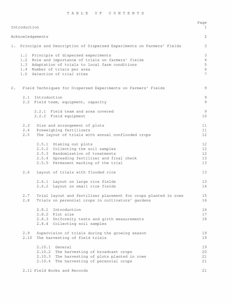
T A B L E 0 F C 0 N T E N T S

PageIntroduction 1

Acknowledgements 2

l. Principle and Description of Dispersed Experiments on Farmers’ Fields 3

l.l Principle of dispersed experiments 3 1.2 Role and importance of trials on farmers’ fields 4 1.3 Adaptation of trials to local farm conditions 5 1.4 Number of trials per area 6 1.5 Selection of trial sites 7

2. Field Techniques for Dispersed Experiments on Farmers’ Fields 9

2.1 Introduction 9 2.2 Field team, equipment, capacity 9

2.2.1 Field team and area covered 9 2.2.2 Field equipment 10

2.3 Size and arrangement of plots 11 2.4 Preweighing fertilizers 11 2.5 The layout of trials with annual nonflooded crops 12

2.5.1 Staking out plots 12 2.5.2 Collecting the soil samples 12 2.5.3 Randomization of treatments 12 2.5.4 Spreading fertilizer and final check 13 2.5.5 Permanent marking of the trial 13

2.6 Layout of trials with flooded rice 13

2.6.1 Layout on large rice fields 13 2.6.2 Layout on small rice fields 14

2.7 Trial layout and fertilizer placement for crops planted in rows 15 2.8 Trials on perennial crops in cultivators’ gardens 16

2.8.1 Introduction 16 2.8.2 Plot size 17 2.8.3 Uniformity tests and girth measurements 18 2.8.4 Collecting soil samples

2.9 Supervision of trials during the growing season 19 2.10 The harvesting of field trials 19

2.10.1 General 19 2.10.2 The harvesting of broadcast crops 20 2.10.3 The harvesting of plots planted in rows 21 2.10.4 The harvesting of perennial crops 21

2.11 Field Books and Records 21

Contents (cont.) Page

3. Designs, Fertilizer Rates and Statistical Checks 32

3.1 Introduction 32

3.1.1 Statistical checks 32 3.1.2 Significance levels 33

3.2 Choice of fertilizer rates for trials on cultivators’ fields 34

3.2.1 General 34 3.2.2 How to choose rates for trials in unknown areas 36 3.2.3 Observations on actual fertilizer rates for experiments 36

3.3 Choice of experimental designs for trials on farmers’ fields 37

3.3.1 Fertilizer rate trials 37

3.3.1.1 General 37 3.3.1.2 Number of treatments 37 3.3.1.3 Designs for two effective and one usually ineffective nutrient 39 3.3.1.4 Designs for three effective nutrients 44 3.3.1.5 The problem of the fourth element 50 3.3.1.6 Experimental designs for perennial crops 51

3.3.2 Nutrient carrier comparisons 52 3.3.3 Other trials with fertilizers 53

3.3.3.1 Time of application trials 53 3.3.3.2 Residual and cumulative fertilizer effects 53 3.3.3.3 Trials comparing fertilizer placement with broadcasting 54 3.3.3.4 Combined fertilizer variety trials 54

3.3.4 Some remarks on designs 55

4. Presentation and Interpretation of Results 56

4.1 General 56 4.2 Work sheets and summary tables of results 56 4.3 Interpretation of results 59

4.3.1 General 59 4.3.2 Analysis of results 59 4.3.3 High profit and high return recommendations 61

5. The Use of Yield and Profit Functions 64

References 65

Contents (cont.)

APPENDIXES Page

I. Calculation of a Parabolic Return Curve from Fertilizer Rates 0, 1, 2 and Relation Between Yield and Profit Functions 66

II. Calculation of the Nearest Surface for Design II 69

III. Calculation of the Neareat Parabolic Return Curve from More than Three Observation Points 71

IV. Calculation of the Neareat Surface for Design III 72

V. Calculation of the Nearest Surface for Design IV: Complete Factorial 3 2 73

VI. Calculation of the Nearest Surface for Design VII 74

VII. Calculation of the Nearest Surface for Design VIII 76

VIII. Calculation of the Nearest Surface for Design IX: Complete Factorial 3 3 77

N 0 T E ========

FERTILIZER TERMINOLOGY

(Expression of Plant Nutrients)

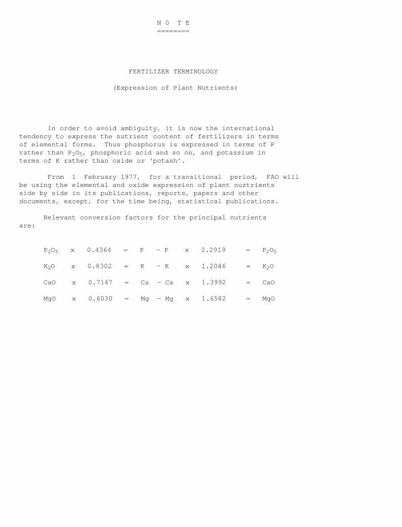
In order to avoid ambiguity, it is now the internationaltendency to express the nutrient content of fertilizers in termsof elemental forms. Thus phosphorus is expressed in terms of Prather than P 2O5, phosphoric acid and so on, and potassium interms of K rather than oxide or ‘potash’.

From 1 February 1977, for a transitional period, FAO willbe using the elemental and oxide expression of plant nuztrientsside by side in its publications, reports, papers and otherdocuments, except, for the time being, statistical publications.

Relevant conversion factors for the principal nutrientsare:

P 2O5 x 0.4364 = P - P x 2.2919 = P 2O5

K 2O x 0.8302 = K - K x 1.2046 = K 2O

CaO x 0.7147 = Ca - Ca x 1.3992 = CaO

MgO x 0.6030 = Mg - Mg x 1.6582 = MgO

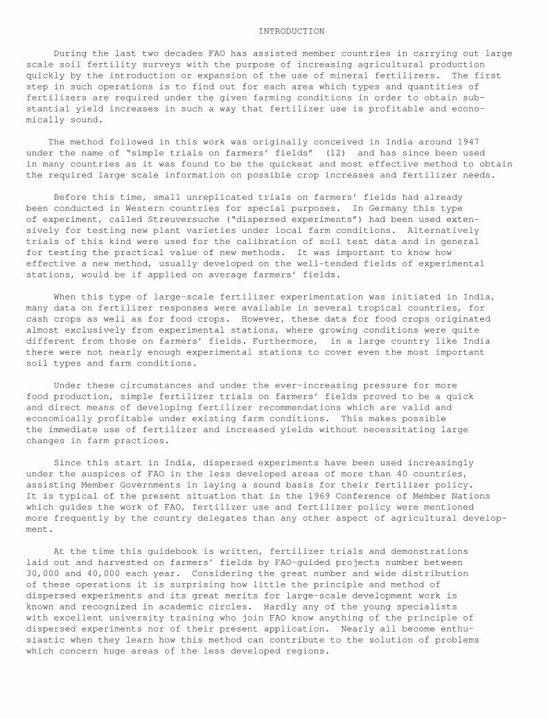
INTRODUCTION

During the last two decades FAO has assisted member countries in carrying out largescale soil fertility surveys with the purpose of increasing agricultural productionquickly by the introduction or expansion of the use of mineral fertilizers. The firststep in such operations is to find out for each area which types and quantities offertilizers are required under the given farming conditions in order to obtain sub-stantial yield increases in such a way that fertilizer use is profitable and econo-mically sound.

The method followed in this work was originally conceived in India around 1947under the name of “simple trials on farmers’ fields” (12) and has since been usedin many countries as it was found to be the quickest and most effective method to obtainthe required large scale information on possible crop increases and fertilizer needs.

Before this time, small unreplicated trials on farmers’ fields had alreadybeen conducted in Western countries for special purposes. In Germany this typeof experiment, called Streuversuche (“dispersed experiments”) had been used exten-sively for testing new plant varieties under local farm conditions. Alternativelytrials of this kind were used for the calibration of soil test data and in generalfor testing the practical value of new methods. It was important to know howeffective a new method, usually developed on the well-tended fields of experimentalstations, would be if applied on average farmers’ fields.

When this type of large-scale fertilizer experimentation was initiated in India,many data on fertilizer responses were available in several tropical countries, forcash crops as well as for food crops. However, these data for food crops originatedalmost exclusively from experimental stations, where growing conditions were quitedifferent from those on farmers’ fields. Furthermore, in a large country like Indiathere were not nearly enough experimental stations to cover even the most importantsoil types and farm conditions.

Under these circumstances and under the ever-increasing pressure for morefood production, simple fertilizer trials on farmers’ fields proved to be a quickand direct means of developing fertilizer recommendations which are valid andeconomically profitable under existing farm conditions. This makes possiblethe immediate use of fertilizer and increased yields without necessitating largechanges in farm practices.

Since this start in India, dispersed experiments have been used increasinglyunder the auspices of FAO in the less developed areas of more than 40 countries,assisting Member Governments in laying a sound basis for their fertilizer policy.It is typical of the present situation that in the 1969 Conference of Member Nationswhich guides the work of FAO, fertilizer use and fertilizer policy were mentionedmore frequently by the country delegates than any other aspect of agricultural develop-ment.

At the time this guidebook is written, fertilizer trials and demonstrationslaid out and harvested on farmers’ fields by FAO-guided projects number between30,000 and 40,000 each year. Considering the great number and wide distributionof these operations it is surprising how little the principle and method ofdispersed experiments and its great merits for large-scale development work isknown and recognized in academic circles. Hardly any of the young specialistswith excellent university training who join FAO know anything of the principle ofdispersed experiments nor of their present application. Nearly all become enthu-siastic when they learn how this method can contribute to the solution of problemswhich concern huge areas of the less developed regions.

Scientifically the method of dispersed experiments is not new. It is thepractical value and large scope of application which make this method a majortool of agricultural development. If this guide encourages the inclusion ofthis type of applied research in the curricula of agricultural teaching, it willhave fulfilled an additional purpose.

Readers interested in more detailed statistical treatments of subjectsmentioned in this guide are referred to the FAO publication “Statistics of CropResponses to Fertilizers” revised edition, 1970.

Acknowledgements

The author wishes to express his gratitude to all those who contributedto this guidebook by providing constructive criticism and comments. Amongthose who worked with FAO on soil fertility problems in various countries duringthe time this guide was written, special acknowledgement is due to:

J.J. Doyle, M.F. Chandraratna, E.W. Boswinkle, H.N. Mukerjee, J.M.P. Memoria, T.P. Abraham, J.W. Dewis, V.D. Thawani, and T. Prasad.

l. Principle and Description of Dispersed Experiments on Farmers’ Fields

l.l Principle of dispersed experiments

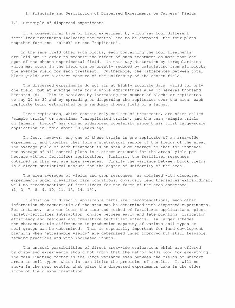
In a conventional type of field experiment by which say four differentfertilizer treatments including the control are to be compared, the four plotstogether form one “block” or one “replicate”.

In the same field other such blocks, each containing the four treatments,are laid out in order to measure the effect of such treatment on more than onespot of the chosen experimental field. In this way distortion by irregularitieswhich may occur in the field can be greatly reduced by calculating from all blocksthe average yield for each treatment. Furthermore, the differences between totalblock yields are a direct measure of the uniformity of the chosen field.

The dispersed experiments do not aim at highly accurate data, valid for onlyone field but at average data for a whole agricultural area of several thousandhectares (6). This is achieved by increasing the number of blocks or replicatesto say 20 or 30 and by spreading or dispersing the replicates over the area, eachreplicate being established on a randomly chosen field of a farmer.

These replicates, which contain only one set of treatments, are often called“simple trials” or sometimes “unreplicated trials”, and the term “simple trialson farmers’ fields” has gained widespread popularity since their first large-scaleapplication in India about 20 years ago.

In fact, however, any one of these trials is one replicate of an area-wideexperiment, and together they form a statistical sample of the fields of the area.The average yield of each treatment is an area-wide average so that for instancethe average of all control plots is a direct estimate for the areas’ yield perhectare without fertilizer application. Similarly the fertilizer responsesobtained in this way are area averages. Finally the variance between block yieldsis a direct statistical measure for the degree of uniformity of the area.

The area averages of yields and crop responses, as obtained with dispersedexperiments under prevailing farm conditions, obviously lend themselves extraordinarywell to recommendations of fertilizers for the farms of the area concerned(l, 3, 7, 8, 9, l0, 11, 13, 14, 15).

In addition to directly applicable fertilizer recommendations, much otherinformation characteristic of the area can be determined with dispersed experiments.For instance, one can learn the time and method of fertilizer applications, plantvariety-fertilizer interaction, choice between early and late planting, irrigationefficiency and residual and cumulative fertilizer effects. In larger schemesthe characteristic differences in production capacity of various soil types orsoil groups can be determined. This is especially important for land developmentplanning when “attainable yields” are determined under improved but still feasiblefarming practices and with increased inputs.

The unusual possibilities of direct area-wide evaluations which are offeredby dispersed experiments should not imply that the method holds good for everything.The main limiting factor is the large variance even between the fields of uniformareas or soil types, which in turn limits the precision of results. It will beshown in the next section what place the dispersed experiments take in the widerscope of field experimentation.

1.2 Role and importance of trials on farmers’ fields

During the last ten years “simple trials on cultivators’ fields” have beenconducted in a quickly increasing number (l, 3, 7, 8, 9, 10, 11, 13, 15), andmany questions have been raised about their merits. Sharp criticism has beenleveled at the lack of precision in this type of experiment because of the greatvariability between fields and the impossibility of fully controlling the growingconditions of the crop. But the method has also had support. Some have gone sofar as to say that any improvement such as fertilizer application should be triedunder average field conditions rather than under the highly controlled conditionsof the experimental station. They reason that only trials under actual farm con-ditions give the necessary insurance that the improvement will be effective andto what extent. Both approaches have their merits; choice should be made accordingto the objectives of the investigation.

The previous section makes it evident that for the decision regarding generalfertilizer recommendations to be used by farmers, exact field experiments understrictly controlled conditions are less important that the dispersed experimentson farmers’ fields.

Because of the great variation between farmers’ yields within an area, smalldifferences between treatments cannot be detected, but these are not required ifsafety margins of 50 percent and more are applied in calculating the fertilizerrecommendations (a benefit/cost ratio of 2 is usually considered the minimum).Sometimes, however, we wish to know small differences with precision and in thesecases exact experiments under controlled conditions are required. An exampleillustrates this case: In comparing fertilizer carrier materials such as ureaand ammonium nitrate the yield differences found in trials on cultivators’ fieldsare usually negligible, but economically urea is usually better because it is cheaperper kilogram of nitrogen. This result may be satisfactory for practical purposes,but still we are interested to know whether the physical crop responses for the twomaterials are really equal. For this, exact experiments are needed. If they showthat one or the materials has a slightly and consistently higher effect on a givencrop, then we can apply this knowledge to advantage if prices for the two materialson a nutrient basis become equal. In this case the country may gain greatly byusing the more effective material, even if the difference is only 2 or 3 percent,a difference which cannot normally be detected on cultivators’ fields.

Both the exact experiments as well as those under farm conditions have givena wealth of information during the last two decades. Each approach has its ownpurpose and one cannot replace the other, as their aims are altogether different.

This relationship between the two experimental approaches explains certainpeculiarities which have often been questioned.

The effects of fertilizer on crop yields are always measured by determininga response curve which shows the increase of yields with increasing rates of ferti-lizer application. While in the exact research experiments the aim is nearly alwaysto get a fairly complete picture of this curve extending from the zero input pointto that of maximum yield and over, the trials on cultivators’ fields are much morelimited in their purpose. With these trials the point of greatest interest isthe application rate at which the maximum monetary profit per hectare is obtainedand the surrounding zone in which this point might move with changing cost-pricerelations.

Another figure that is most important to the farmer and the government isthe monetary return per invested capital, called value/cost ratio. Obviouslysmaller fertilizer rates result in higher returns per money invested. Apartfrom exceptional cases, a farmer is not interested in a maximum yield because itusually requires an uneconomically high fertilizer application. It is simplytoo expensive.

For these reasons it will be found that in the following pages maximum yieldsare rarely mentioned while all efforts are directed toward obtaining, in thesimplest way, the points on the return curve of highest profit per hectare andhigh returns per invested capital. It would be a waste of effort and money todetermine in many hundreds of trials per area a larger part of the return curvethan is required for finding these points. Therefore, only in exceptional casesdo the results of these trials allow the determination of the maximum yieldwithout exessive extrapolation.

1.3 Adaptation of trials to local farm conditions

The trials carried out on cultivators’ fields are made in order to developrecommendations which are fully valid under these conditions. However, in practicalexecution one finds that farm conditions vary greatly not only from coumtry tocountry but also from area to area within a country. In many instancea traditionalfarming practices are used-timely weeding by hand and timely irrigation, for example.When well done, these make excellent conditions for applying fertilizers, and inthese favourable cases there is no pressing need to improve the farm practices whencarrying out trials. However, while doing such development work with a farmer onhis own fields, there is a good opportunity to advise on possible improvements,such as using highly responsive varieties, protecting plants against diseases andpests, improving irrigation, and whatever other local possibilities there may be.If the farmers are receptive and apply such additional improvements, they shouldimmediately be included in the trials. Such improvements can also be introducedin the trials before the farmer adopts them; in this case the trials will serveexcellently as demonstrations and, at the same time, will measure the effects ofthe improvements.

In cases where farm practices are extremely poor and essentials such as weedingor proper plant protection are neglected, the crop plants often will not be able tobenefit from the applied fertilizers. It would be of little use to make fertilizertrials under such conditions.

If these conditions are found only on few of the farms in an area, these farmsshould be excluded from the trial programme as they would unduly depress area averages.The farmers should be advised not to use fertilizer until general farm practicesare such as to produce normal healthy crops.

The large majority in any country or area will of course have conditions inbetween these two extremes, and in these average cases it is always necessary tourge farmers to apply further improvements within their reach besides fertilizers.The good results from fertilizers give the farmers confidence, so that pleasfor certain additional improvements will often be successful. Naturally this isfacilitated if such improvements are demonstrated to the farmer by including themin the fertilizer trials.

In areas where basic information has already been obtained by trials underexisting farming conditions during several seasons, more advanced research isrequired, in order to obtain information on higher or highest “attainable yields”.

Such attainable yields are also determined with trials on farmers’ fieldsby applying that farm management level and those amounts of inputs (kept as uniformas possible) which are expected to lead to high economic outputs.

In such experiments small machines may be used to obtain a uniformly wellprepared seedbed. Irrigation will be improved. Improved seed varieties are used.Fertilizer rates will be increased and plants protected against pests and diseases.The farmers will observe such experiments with greatest interest if the scope ofimprovements is not too far out of their reach.

1.4 Number of trials per area

It is a general rule that the precision of an experiment increases with thenumber of replications. In our case, the number of trials to be laid out dependsof course on the size of the area. We will see later that a field team of fourpersons can cover an area of 60,000 to 100,000 hectares and even more. Such largeareas are never uniform, and it is not only convenient but even necessary to dividethem into subareas such that each subarea, judged from an agricultural and soilspoint of view, is as uniform as possible. Such subdivision is also convenient,as each team member can take one subarea under his special supervision.

If there are four subareas and the team’s total capacity is 100 trials perseason, about 25 trials per season per subarea of l5,00O to 25,000 ha are laid out.Such a coverage has proved satisfactory in all cases. (See also 2.2.1).

For special trials with annual crops for which not much effort is to be made(meaning a minimum number of trials), it is a rule based on experience that theminimum number of established trials for each set should be not less than 12 andthe number of well conducted harvested trials not less than 10, allowing for twounforeseen failures.

Such and larger trial sets have a high chance to give statistically convincingresults, while this is not the case with smaller sets.

There are also mathematical approaches by which one calculates in advancethe number of trials needed for obtaining results of a certain precision. Thesecalculations are little used since the basic information required is seldomavailable. As a demonstration the simplest approach is shown here.

Referring to the analysis of variance, the mean square of the error is usuallycalled s 2. The standard error of the mean (SE) is then SE = s/n½ where n isthe number of replicates (trials). If we express the standard error in percentof the mean yield M, then we obtain SE % = s.100 . M.n½

The coefficient of variation (CoV) is: CoV = s.100 % M

Therefore SE % = CoV and n½

n = ( CoV ) 2

(SE%) 2

The experimenter can estimate for a certain planned set of trials the coeffi-cient of variation. Then he must choose the maximum permissible error, expressedas percent of the mean. With these two figures he can calculate the required numberof trials. For a more detailed mathematical treatment see the FAO publication“Statistics of Crop Responses to Fertilizers”, revised edition.

Under given conditions the coefficient of variation is very characteristicfor each crop. Its estimate is simple and for an experienced experimenter ratherprecise. This is not so with the estimate of the required maximum error. Onemight not be able to estimate the control yield in an unknown area, and even lessthe fertilizer response. Without knowing the magnitude of the response it isimpossible to set the maximum error in percent which would give significant results.

In the practical execution of projects the number of trials per set dependson the work capacity of the field teams and the extent of the experimental programme.The latter should not be over-ambitious. Relatively more trials should be assignedto the most important experimental sets, keeping the above-mentioned 12 establishedtrials as a minimum per set in cases of orientation experiments.

1.5 Selection of trial sites

According to the principle of dispersed experiments as explained in Sectionl.l, the fields on which the replicates of the area-wide experiment are laid outshould represent an unbiased field sample of the area. Therefore, the fields shouldbe selected at random.

This principle holds good for areas as a whole or for certain parts of an area.It is often necessary to group the area’s fields into “strata”, for instance if partof the fields are irrigated and other parts are not. Separate trial sets are neededfor these strata, and the random selection of fields is of course done within eachstratum separately. Salinity might be another criterion for strata distinction.In all cases the trial sites within a stratum have to be selected at random.

The methods employed to achieve such a selection may vary. In order to givethe reader an impression of which methods were tried, some of them are briefly describedbelow although they are not recommended for use:

l. Compiling an inventory of all fields of the area and making a random selection in the office

2. Compiling a list of all farmers in the area and selecting some at random.

3. Working with a detailed map of the area and selecting fields by randomly chosen coordinates.

One can, of course, invent more such systems but their practical value isdoubtful for several reasons. For instance, with regard to 1 and 2, the compilationof inventories is a major undertaking and in developing countries is often impossible.

Furthermore, a trial can only be laid out if a farmer agrees to it. In discussionof this point often the mistake is made of calling farmers “progressive” who agreeto the layout of a trial, and it is said to be a major bias that all trials arelaid out on progressive farmers’ fields. This picture is not true to fact. Amongthe more progressive as well as the less progressive farmers there are some whosay yes and others who say no. Their decision depends largely on their confidencein the project’s field staff, as can be seen from the fact that after the firstseason or two, when farmers trust the staff and see the value of the work, a refusalto accommodate a trial is an exception (13).

Another factor in the equal distribution of trials over the area is theinaccessibility of certain fields. A map of the area on which the trial sites aremarked will allow the uniformity of distribution to be judged. Leaving out partsof the area which are inaccessible or difficult for the field team to reach isoften regarded as a bias in the selection of fields. This is not necessarily soand the need for making trials in such spots, involving sometimes high costs andmuch effort, can be judged beforehand from a visit of a soil specialist to checkon the comparability of soils and conditions with neighbouring accessible areas.If the soil conditions and farm practices are the same, there is no need to maketrials on the inaccessible fields.

In all larger FAO projects involving area-wide dispersed experiments theimportance of the following principle in selecting fields is recognized:“A choice of a field is unbiased if the chooser does not know beforehand whatkind of field he selects.” This principle has proved to be true for all practicalpurposes, although it is well understood that biasses can never be avoided completelyas may be required by statistical theory. Because the principle cited is practicallytrue, all the systems mentioned in the end gave good results. (The criterion forcalling a system “good” may be taken in this case as the consistency of resultsobtained over the seasons.) Expressed more critically, one can say that no indi-cations have been observed suggesting that one system of random selection is betterthan another and it is most unlikely that such differences will ever be found.

As the fields are selected before ploughing when they are bare, there ispractically no chance of a bias. Statistically speaking the chance of bias inselecting fields by going from one spot to the next (which should not be lessthan one kilometer away) and picking fields at random is practically zero.This is because the variation of yields between sites is large and a distinctionbetween good and bad fields on sight rarely possible.

Taking all these facts into consideration, it is recommended that fieldsbe selected on the following lines which were approved at the project managers’meeting in the Far East (1967) when 15 senior specialists discussed the matter.

Larger areas are divided into subareas in each of which a number of villagesare chosen such that their distribution over the area is as uniform as possible.Fields are chosen at random by the project team in these villages. Of course,the farmers’ agrement is required, but as was pointed out, few farmers will objectafter the first two seasons,

This simple system of a two-stage stratified sampling in which subareas arethe first and villages the second stage has proved efficient, resulting in suitablearea coverage and satisfactory precision.

2. Field Techniques for Dispersed experiments on Farmers’ Fields

2.1 Introduction

According to the principle of dispersed experiments, the accuracy of theresults increases with the increasing number of trials, each of which is a replicateof the area-wide experiment. The work capacity of the available field team musttherefore be used in such a way as to conduct the highest possible number of trialswith the highest possible precision. This can best be achieved by standardizingthe technique for each phase of the work so that in the two seasons of high workpressure, the layout and the harvest, the fully occupied team will handle the samenumber of trials.

In the standard technique to be described, this equilibrium is reached notby harvesting whole plots but by taking good-sized harvest samples. By trying toharvest whole plots the team will not be able to do as many trials in the relativelyshort harvest period, the field sample of the area will be smaller and precisionis lost again. In addition the field team will not be fully occupied during thelayout period.

In practice the equilibrium should be established by laying out, in the caseof annual crops, about 10 percent more trials than can be harvested later.The reason for this is of course that during the growing season a number oftrials are always lost by influences beyond control. The extra trials willensure that time is fully utilized during the harvest.

In later seasons when the field assistants are fully trained, and are wellacquainted with all phases of the work, the operations can be facilitated con-siderably and the total travel mileage reduced by posting each assistant in a subarea,where he is in charge of making the arrangements with the farmers and supervisingthe trials. For the layout, harvest, and threshing the team works with the responsibleteam leader.

2.2 Field team, equipment capacity

2.2.1 Field team and area covered

A suitable field team consists of one team leader, two or three field assistants, and one or two untrained labourers or farm hands. The team works with one field car.

A team of this composition is able to lay out 80-120 standard wheat trials of 12 plots each in one planting season if the work has become a well settled routine in which every team member knows what to do. In areas with scattered districts involving long journeys, the number of trials which can be laid out will be nearer to 80 and in the compact areas over 100. The same team will be able to harvest between 70 and 110 trials without extra effort, thus leaving a certain margin for unavoidable losses.

With regard to other annual crops such as sugar beets, cotton and rice, the number of trials to be handled will be somewhat lower, varying mainly with the work involved in the harvest.

In countries of the Middle East where wheat and barley are winter crops planted in the fall and harvested in early summer and where other annual crops are planted in the spring sad harvested from late summer to winter, the team can lay down and harvest up to 180 trials in the two seasons of one year.

A good coverage of an area would be one trial per 600-1,000 hectares per season. A team can, therefore, cover 60,000-100,000 hectares of arable land depending on whether the area is scattered or compact. The trials should be conducted with each main crop for not less than three, and even better four, years which will result in the very satisfactory coverage of 150-200 hectares per trial.

Unavoidable losses of trials vary a great deal from area to area. In general they are high in the first season but decrease in later seasons, with increasing experience of farmers and field teams.

2.2.2 Field equipment

The field equipment required for each team for the layout and harvest of the trials includes the following items:

l. Two steel or plastic measuring tapes of 50 and 30 m respectively.

2. Rough wooden sticks 60-7O cm long; 21-26 of these are required for each trial of 12 plots.

3. Four to six straight sticks 150-170 cm long.

4. A heavy hammer for driving sticks into the ground.

5. Right angle mirror or prism. If this is not available a loop of rope holding three rings can be used. The rings are fixed at measured intervals such that when the loop is extended to form a triangle, with the rings at the corners, a right angle will be formed. (For example, intervals of 3, 4 and 5 meters.)

6. Cotton rope 5-8 mm thick, four lengths of 50 m each.

7. Two plastic buckets for spreading fertilizer on the plots.

8. One plastic bucket kept absolutely clean for collecting soil samples.

9. A piece of canvas for mixing soil samples to attain a composite sample.

10. A simple compass.

11. A field book.

12. Bags with preweighed fertilizer.

Items for harvest

13. Large bags for collecting grain, at least one for each plot.

14. Two scales sturdy enough to stand travelling, the lighter type with a capacity of 3-5 kg for cotton picking or grain samples, the heavier type with a capacity of 50-100 kg for sugar beets or fruit. Steel yard scales are often suitable since they are light and sturdy.

15. Threshing machine for plots of small grain. Hand threshing is possible.

2.3 Size and arrangement of plots

The choice of a standard plot size is of great importance for each project,and the chosen size should be used for as many crops and trials as possible.An exception is submerged rice (described under 2.6). If various annual cropsare included in the programme, a standard size of 50 sq m (10 x 5m) is mostconvenient and would also accommodate crops like cotton for which larger harvestareas are used. For small grain one can go down to sizes of 30 sq m. However,for the smooth and easy layout of many trials per season varying plot sizes area source of repeated mistakes. Standard plot sizes are also required for thepreweighing of fertilizers, and the work of the teams is much more reliable ifthe plot size is always the same.

The plot arrangements in a given field may vary with the shape of the field,the slope or irrigation system. No fixed rule can be given. Compact arrangementsby laying out two rows of six plots each or three rows with four plots each arepreferable to arrangements where all plots are in one long row. Less compactplot arrangements may have a slightly higher variance between plots, but this isof very little influence on the results, since this variance is much lower thanthat between sites.

A separation of plots by ridges or open strips is not needed except in thecase of submerged rice. After being spread on the ground the fertilizer shouldbe quickly covered by soil, either by ploughing it under with the seed or by aharrow or light disc. If this is done, irrigation will not shift the fertilizer.Irregularities along the edges of plots are cancelled out by not harvesting thewhole plots. In the case of top dressings in irrigated crops, ridges betweenthe plots are required because of run-off from one plot to the next, which mustbe prevented. Therefore in the case of top dressings each plot should be irri-gated directly from the irrigation canal.

2.4 Preweighing fertilizers

It is an advantage to weigh the fertilizers for the field plots in the officewhen work pressure is low before the season begins. In this way, too, weighingerrors in the field can be avoided. However, fertilizer bags are easily mixed upand it is advisable to have small bags of three different colours, for instancered for nitrogen, blue for phosphorous, and white for potassium. In each bag theamount of fertilizer is weighed corresponding to only the lower application rate(N 1, P l , K l ) for the standard plot size. If on a certain plot the higher rate,

say N 2, is needed, two red bags will be used. This procedure has the advantagethat checks are possible until the last moment as describeb under 2.5.4.

2.5 The layout of trials with annual nonflooded crops

2.5.1 Staking out plots

The seed bed is prepared by the farmer who agrees to start seeding his field immediately after the fertilizer is spread on the plots. This is then followed by- covering fertilizer and seeds with soil in the usual way. If nitrogen fertilizer is not covered soon after spreading, appreciable amounts of nitrogen will be lost.

The position of the plots in the field is decided by the team leader who puts a long wooden stick into the soil at the nearest left-hand corner of the trial. From this “left point” the two measuring tapes are rolled out by two assistants in perpendicular directions. One assistant marks the end of the base line with a long stick, and the other is directed by the team leader with the help of the right-angled prism to the exact third corner of the field. Leaving the tapes on the soil, one or two other men put small sticks in the soil to mark plot corners at proper distances along both tapes. After this has been done each tape is carried over to the opposite side, completing the rectangular shape of the trial. Again corner points of all plots are marked along the two tapes by sticks driven firmly into the soil with a hammer. The ropes are then pulled around the sticks in a meander form and in this way will mark the plots. Now the corner points inside the field separating two rows of plots are marked by small sticks. The ropes are left in place until the spreading of fertilizer is finished. The team leader makes a sketch of the trial in his field book showing the north direction and some landmarks which will help him to find the trial later on.

2.5.2 Collecting the soil samples

From each trial a composite soil sample is taken for chemical soil tests. As soon as the corners of the trials are marked, one man with a plastic bucket carefully kept clear of any contact with fertilizer and with a clean auger or small spade collects about 20 topsoil samples of equal size from points equally distributed over the trial area. The soil is then throughly mixed on a clean piece of canvas, and one kilogram of the mixture is put in a clean bag to be taken to the soil laboratory. The depth of sampling is the thickness of the topsoil down to the plough sole.

2.5.3 Randomization of treatments

From an ordinary pack of cards one card for each treatment is taken and marked. The team leader shuffles these cards and starting from the left point assigns to the plots in sequential order the treatments drawn from the pack. While he is calling out these treatments the assistants put the appropriate preweighed bags of fertilizer on each plot and the team leader notes the treatments in the field book. One can also randomize treatments in the field office in advance, using random figure tables.

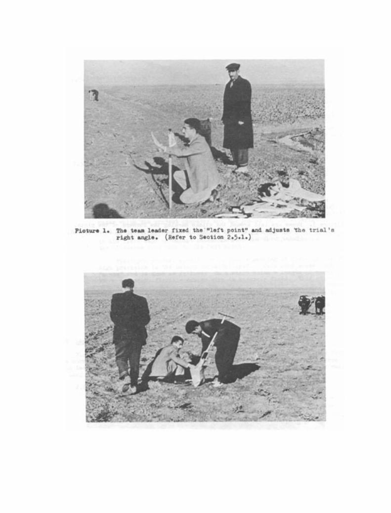
Pioture 1. The team leader fixed the'"left point" and adjuete the trtal'nright angle. (Refer to Seotion 2.5.1.)

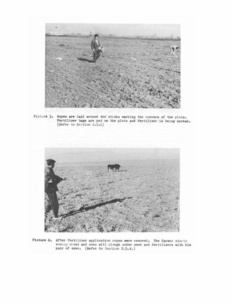
Pictur 3. Ropes are laid .round the sticks narking the corners of the p/ots.Fertilizer bags are put on the plots and fertilizer ia helm spread.(kofer to Section 2.5.4)

046.

.4'

Picture 4. After fortiliter application ropes were removed. The farmer etmrtasowlug 141eat and soon will plough under seed and fertilizers with hispalr of ozen. (ksfor to Section 2.5.4.)

2.5.4 Spreading fertilizer and final check

The assistants now empty the fertilizer bags for each plot into a bucket, add a little dry soil if the quantity is too small, mix thoroughly and distribute it equally over the plot. It is important that they leave the empty bags on the plot. The team leader, after the work is finished, again goes over the field and compares his notes with treatments of the plots which are indicated by the bags. This final check makes it possible to discover and correct mistakes. Now the ropes and bags are removed and the farmer should start seeding and harrowing.

2.5.5 Permanent marking of the trial

In order to find the trial early at the time of harvest when the field is hidden under the crop some precautions are necessary. One possibility in an arid climate is to surround the left-point stick with a layer of gypsum powder. This will stay in place for the whole season and even if the stick is removed the field can be located. If the farmer agrees, it is a better method to have a high signboard put in the corner of a field showing the government organization under which the project operates and the number of the experiment.

An additional security measure is for the team leader to mark in his field book permanent landmarks near the trial, measuring the distances from them to the left point.

Finally a special method for long-term marking of field trials with high precision is the method called “micing”. This name comes from “mouse” and is done as follows: On a short stick a length of about 70 cm of tough, flexible copper wire is securely fixed. This stick is then driven into the ground at the corner of the field to such a depth that its top is safely below the plough sole, while the wire lies on the soil surface. If this spot is properly marked with regard to permanent landmarks, the wire can always be found even after years of regular field operations, and the exact position of the trial is then known. This is especially important for residual effect trials.

2.6 Layout of trials with flooded rice

Flooded rice is grown under varied conditions. On flat terrain the rice fieldsare normally large, while on sloping land usually terraces are made which narrowwith increasing steepness of the slope. The fields on the terrace are mostly small,or long and narrow.

2.6.1 Layout on large rice fields

In plains or on broad terraces trials can be laid out on the large paddy fields similar to those for nonflooded crops, as was described earlier. At the layout of trials the rice fields are usually wet from ploughing and puddling. Nylon measuring tape and nylon rope should be used and rubber boots are needed by the field staff.

A composite soil sample is taken as has been described under 2.5.2. As the soil is usually wet, a plastic bag must be used for the sample. Depending on the instruction of the soil chemist, the soil sample should either be airdried at the field station as soon as possible or it should be brought immediately to the soil test- ing laboratory in its original wet condition.

When such trials are staked out the plots must be separated from each other by the usual ridges. Before applying the fertilizer one should make sure no water is flowing in or out of the plots and the ridges are safely closed. Then the fertilizer is spread on the plots, using preweighed fertilizers. Ideally, transplanting should start immediately or very soon after the application of the ferti- lizer. If the puddles have disappeared the water stream can be started slowly. With this precaution, the dissolved fertilizer will penetrate deeper into the soil and will not be displaced horizontally by the water movement. If the plots are completely flooded the normal water stream can be established.

In the case of top dressing essentially the same procedure is to be followed. First the water flow is stopped completely, then the fertilizer is spread into the standing water. The ridges must be kept closed until all the water has soaked into the soil, and they should be left closed for a few hours afterwards. Thereafter the water stream is started again slowly and after flooding the plots the normal stream is established.

2.6.2 Layout on small rice fields

In the case of small fields on terraces it is usually not possible to lay out rectangular plots of the normal size nor is it always possible to accommodate a whole trial in one field. In this case a group of small neighbouring fields is selected, each of which can be used for one or more plots. The plot size may vary between 30 and 60 sq m. If, for instance, a field has approximately 80 sq m it is divided by a ridge into two approximately equal pieces. Extremely irregularly shaped fields should not be included in the experiment.

After having established in this way the required number of plots (which should be as close together as possible) a composite soil sample is taken as described previously. A sketch of the trial is now made in the field book and the surface area of each plot is determined. If the plots are rectangular, length times width will give the surface area. Often, however, the opposite sides are not parallel. In this area. Often, however, the opposite sides are not parallel. In this case the average length of the plot is determined by adding the two long sides and dividing the sum by two. The average width is calcu- lated in the same way. The average length times the average width then gives the surface area. (This is an approximation sufficiently accurate for the purpose.)

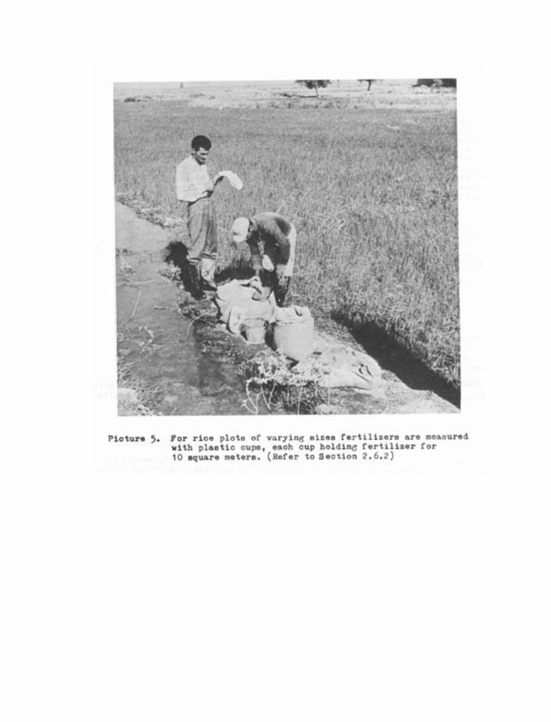
Pioture 5. For rice plots of varying wizen fertilizers ere mcanuredwith plaatic cupe, ach cup holding fertilizer for10 square metern. (Refer to Section 2.6.2)

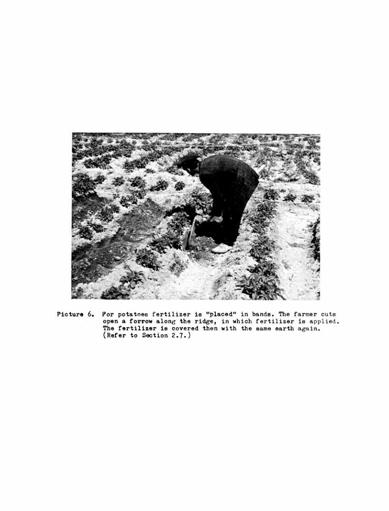
Picture 6. Por potatoes fertilizer in "placed" in bands. The farmer cutsopen a forrow along the ridge, in which fertilizer is applied.The fertilizer in covered then with the same earth again.(Refer to Section 2.7.)

Each plot of such a trial has a different surface area, but it would be impractical to calculate and weigh fertilizer for each plot separately. Therefore the fertilizers are measured by volume. In order to do this, cheap plastic cups are calibrated beforehand by cutting them to such a size that they will hold the lower standard fertilizer rate for 10 sq m of field. For instance, if urea (46%) is used and the standard rate N l is 40 kg N/ha than 10 sq m will need 40 g pure N or 87 g of urea. Therefore, the cup for urea must hold just 87 g if it is brimful. It is obvious that a separate cup must be calibrated for each type of fertilizer. These cups may be coloured to match the fertilizer bags in order to prevent mistakes.

The procedure will now be clear to the reader. The fertilizer is taken out to the field in bulk, together with the measuring cups. When the plot surfaces have been measured they are entered in the sketch in the field book. The treatments are randomized and also entered in the sketch. Now the team leader measures out the treatment for each plot using the special cups. He empties them directly into a bucket and the assistants spread the fertilizer mixture on the plot assigned to the treatment.

Example

If a plot of 35 sq m should get the treatment 1-2-l, it will require 3 1/2 red cups of nitrogen fertilizer, 7 blue cups of phos- phorus fertilizer and 3 1/2 white cups of potassium salt. If the plot surface is only 32 sq m in size only 3 1/4 cups of nitrogen will be required. Estimates down to 1/4 of a cup are sufficiently accurate for the purpose.

The closing of the water stream before fertilizer application and other precautions as described previously for large fields also apply of course to these experiments on small fields.

2.7 Trial layout and fertilizer placement for crops planted in rows

The placement of fertilizers in bands along plant rows is not only done inmechanized agriculture but also in some types of farming in developing countrieswhere all the work is done in traditional ways with animal draft and by hand.In these traditional systems some crops are always planted in rows such as melons,tobacco, potatoes, and sometimes maize. When farmers started to use fertilizer,for them rather expensive, in order not to waste it they banded it in small hand-made furrows along the tobacco rows or at the foot of potato ridges. In the humidtropics fertilizer placement is an effective means to counteract phosphorus fixationby the soil.

Since the fertilizer trials on farmers’fields should closely follow the localpractice, a method has been worked out which is especially suitable for crops plantedin rows with fertilizer placement. ·

The plot size is again strictly standardized to say 50 sq m. Furthermore thenumber of plant rows per plot must always be the same. For many crops five rowsper plot is suitable. Since plot surface and number of rows are kept constantthe plot length varies with the distance between rows. Say that the average rowdistance is 80 cm, then the plot width is 5 x 0.8 m = 4 meters and the plotlength must be 12.5 meters to obtain the standard plot surface of 50 square meters.

Since in each plot of 50 sq m there are five furrows along the plant rows inwhich the fertilizer must be applied, each furrow must get the amount of fertilizerfor 10 sq m. This fertilizer is not weighed but is measured by volume with thecalibrated plastic cups described for the layout of rice trials on small terracedfields. For each type of fertilizer one cup is calibrated to hold, if brimful,the lower standard nutrient rate for 10 sq m. (See 2.6.2.)

Taking the example given for the rice experiment, the cup holding 87 g of ureaif applied once to each of the five furrows in the plot will result in the appli-cation N 1 of 40 kg N/ha. For the appliaction N 2 or 80 kg N/ha each furrow has toget two cups of urea.

With this method therefore the fertilizer is taken to the field in bulk, eachmaterial with its measuring cup, and the fertilizer is measured for each row intoa bigger container from which after thorough mixing it is distributed uniformlyover the length of the row.

In actual practice the field assistant who distributes the fertilizer will firstdo the two border rows which are not harvested and having gained experience in thisway will achieve a uniform fertilizer distribution in the three middle rows whichare harvested later (see 2.10.3).

In fields where the row planting has been done by hand or with a one-rowseeder the row distances vary to some extent. In this case it is sufficientto determine the average row distance by counting the number of rows over a lengthof 30 to 50 meters on the experimental site and by dividing this distance by thenumber of rows. The resulting average row distance is then used for all plots ofthis trial so that all plots will be the same length. There is no need to measureplots individually as in a set of trials the positive and negative deviations canceleach other out.

2.8 Trials on perennial crops in cultivators’ gardens

2.8.1 Introduction

The obvious difference between trials with perennial and those with annual crops is the duration of the experiment. In the year after the first application of fertilizers the effect on total growth may not be great, although reactions in the colour of foliage may appear in a few days. In the following years when fertilizer applications are repeated regularly, the effects on growth will become more marked. These effects will not necessarily reach a ceiling as is the case with annual crops. Since a tree is growing continually through the years, a regular supply of extra plant food will cause its growth line to be steeper than that of a poorly fed tree. In terms of fertilizer trials this means that the yield differences between plots increase steadily through the years. This increase might reach an end point after many years when the fertilizer supply becomes small for the size of the tree.

Experiments for determining practical fertilizer needs in terms of economy will not reach this end point. They should show good results after three to five years, not counting time needed for the uniformity test (see 2.8.3). Afterwards they can be discontinued or used for other tests. For commercial gardens even this relatively short period of three to five years might be too long, and suitable rental agreements might be needed to ascertain that the experiment can be carried through to its end. Gardens of government-owned experimental and demonstration farms are suitable alternatives only if their treatment during the last years was sufficiently similar to that of the surrounding commercial gardens.

Because of this situation it is advisable to present results of fertilizer trials with perennials also in cumulative growth lines (regression of yield with time), besides the usual yield and response presentations.

Another specific feature of trials with perennial crops is the following: Perennial crops like trees, grapes and tea develop large root systems which reach well into the roots of neighbouring plants on normal plantations. If fertilizer is applied around one tree the neighbouring trees will also profit somewhat from the appli- cation. It is therefore necessary to separate the trial plots by leaving at least one unfertilizer guard row between plots. Only on exceptionally wide-spaced plantations or in the case of young trees may guard rows be unnecessary.

The guard rows increase the number of required trees of each trial considerably. For instance, for twelve plots of six trees each, in a square arrangement, 169 trees are required of which 72 are actually test trees and 97 are for the guard rows. If the plots are decreased to three trees per treatment still 117 trees are required of which only 36 are test trees and the rest guard rows. Eight plots of three trees each in a compact arrangement require 81 trees of which only 24 are test trees. These examples show that many of the smaller gardens in fruit areas may not accommodate trials with twelve plots or more.

2.8.2 Plot size

The figures just given show that the ratio test trees/guard row trees is more suitable if the plots are larger. The first example of six trees per plot was taken because this number is suitable from two angles: 1) the average of six trees results in accuracy which is specially needed in the beginning of the experiment when fertilizer responses are slowly building up and differences between treatments are small, and 2) in later stages of the experiment it often happens that additional deficiency symptoms or other problems develop which require investigation. The plots with six trees lend themselves well to such additional tests. If the trees of the plots are arranged in two rows of three, the two middle trees can be used as guards separating the two remaining pairs of trees. One of these pairs can then receive an extra treatment. Since by the time this additional test is needed the yield capacity of each tree is well known, accurate results from the extra treatment are obtained immediately. The enormous having of time using this system rather than starting a new experiment is obvious.

If in small gardens the plot size is cut down to three trees per treatment the number of guard trees is increased much more than the number of extra plots gained, although such gain can sometimes be important. Also with plots of threes trees in a row extra treatments can be tested by using the middle tree as a guard and applying the extra treatment to one of the two remaining trees. However, one tree per treatment involves uncertainties and the planning of an experiment may preferably be based on a minimum of two trees per plot.

2.8.3 Uniformity tests and girth measurements

Uniformity test.

At the start of an experiment the trees are already developed and have individual yield capacities. Although one will try to select gardens with uniformly developed trees of the same age, individual differences are still considerable.

Since, furthermore, only a few trees can be included in one plot, it is obvious that even under suitable conditions the selected plots will have different yield levels from the start. If fertilizer effects are to be measured with accuracy, these initial yield levels at or before the start of the experiment must be known. Any change in yield of each plot or of each tree can then be measured correctly by the usual co- variance analyses.

The determination of a tree’s initial yield, usually for two years, is called a “uniformity test”.

In carrying out a uniformity test it is necessary to determine not only yields of each plot as a wbole but the yields of each tree separately. There are two reasons for this. First, most fruit trees have marked yield periodicity, with high yields in alternate years. It is an advantage to know the periodicity of each tree as it will often explain irregularities found in yield results. Second, if in later stages of the experiment the plots are split into two parts to test extra treatments, the yield characteristics of single trees are needed.

Girth measurement

The circumference (girth) of the tree trunk, measured at a constant height over the ground (usually 1/2 metre) is an indication of the strength and possibly also the production capacity of the tree. In extensive experiments with apple trees in Iran both uniformity tests and girth measurements have been carried out. It was found that the girths of trees correlated sufficiently with their yield capacities to be taken as the basis for covariance analysis instead of uniformity test yields. This would mean that the lengthy two years of uniformity tests can be replaced by a simple girth measurement of each tree at the start of the experiment and that fertilizer treatments can be applied immediately. The obtained yields must be corrected according to the measured girths by the covariance analysis.

These results obtained in Iran probably can be used in the majority of tree trials with advantage. The two years otherwise used for unifor- mity tests will be added to the measurement of the growth curves per treatment.

Picture 7. A wEent trial on a farmerso field. The two darker nitrogen plots,and between them the no-nitrogen plot are clearly visible.

Picture S.. The harvest frame for nmall rrain io adjuoted precieely to2.5 ic 4 'cetera (10 egare meters) before the harvent otarts.This frame can aleo be uoed for other crops.(Refer to inction 2.10.2)

In both uniformity tests and girth measurements the experimental trees must be numbered individually. Sometimes it is convenient to mark all guard trees with a ring of paint for better orientation in the garden.

In the field book the individual tree numbers are entered in the trial sketch.

2.8.4 Collecting soil samples

For tree crops with large root systems it is not sufficient to collect only one composite topsoil sample as described under 2.5.2. A second composite soil sample should be taken from a depth in the soil where the main part of the trees’ feeder roots are found. This work can conveniently be done with a tube-type soil auger.

2.9 Supervision of trials during the growing season

Once started, the trials must be supervised regularly during the vegetationperiod until the harvest. Each field trial should be visited at least once everyfortnight or more. A record of the development of the crops should be kept bythe assistants carrying out this supervision. This can be done most easily bykeeping a plot score. In the course of the season it will then be seen how thedifferent fertilizer treatments affected growth in the earlier and later stages.During these visits checks should also be made with regard to damage by flooding,animals, or other, and of crop injuries by pests and diseases. Special attentionshould be given to the colour of the crop and leaf symptoms, as they point todeficiency of nutrient elements. Also weed incidence should be recorded. In thecase of small grain it is useful to make tillering counts in selected trials.The time of heading should be recorded from each treatment. In the case of cottonand other crops, time of flowering and other characteristics should be noted.If fields are irrigated the number and dates of irrigations should be carefullyrecorded.

2.10 The harvesting of field trials

2.10.1 General

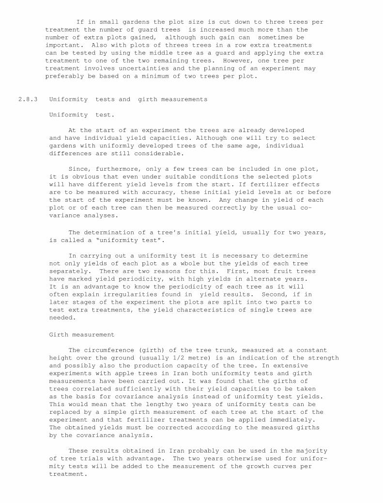
The standard harvesting method as described in this section foresees that only 10 sq m of each plot are harvested, except in the case of cotton where 15-20 sq m are harvested.

The opinion is often heard that the harvesting of whole plots gives more accurate results and would not take much more time than the 10 sq m sampling. This may be true for the experimental station, but it is not so in the practical execution of a country wide project in which the field staff’s working capacity and the funds for operation and extra labour are limited.

With equal staff, funds and facilities, the harvesting of whole plots would cut down the number of possible field trials to half or even less, again with the exception of cotton. The precision gained by whole-plot harvesting is more than lost again by the smaller size of the area sample. The crop sampling allows for the highest number of trials and also for the highest precision.

AL, Lie

t-5,04- e

Picture 9. Omit plots are harvested by cutting out 10 square etres of the °antesof eath plot, putting the sasple in bags. (Refer to Section 2.10.2)

.16, .'4. .111" ' .

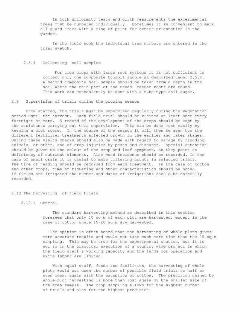
Picture 10. The bags sontaining the harvested wheat samples are brought to thevillags where they remain with the owner until threahing time.(Refer to Section 2.10.2)

**1...:-

- 41b-soks......._"="'-liliata.-_

__

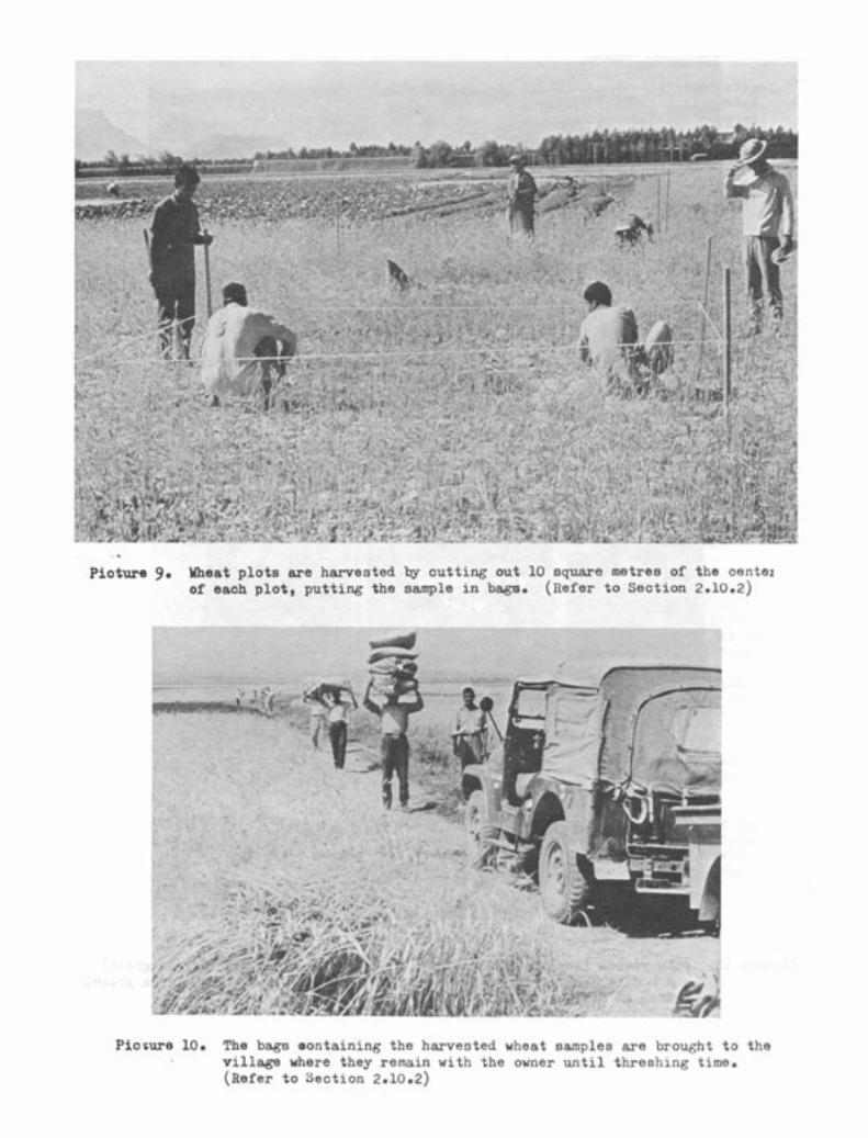
Pioture 11. The experimental yields are threshed with a small machine not requiringcleaning alter each sample. (Refer to Seotion 2.10.2)

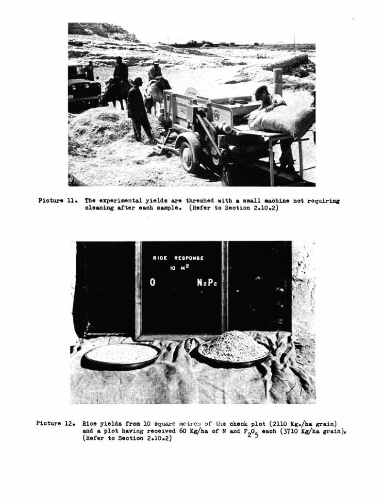
Picture 12. Rice yields from 10 square metre:1 of the check plot (2110 Kg./ha grain)and a plot having received 60 Kg/ha of N and 1)() each (3710 Kg/ha grain),(Refer to Seotion 2.10.2) -

Another advantage of the plot sample of 10 sq m is the elimination of border effects. This means that in all trials including irrigated crops, the plots can be laid out side by side without being separated by ridges. Flooded rice is of course an exception.

2.10.2 The harvesting of broadcast crops

At harvest time an arrangement is made with the farmer to decide the day of harvest. Field trialas should be harvested just before the farmer harvests or even one or two days earlier. In the case of cotton this is especially important because the farmer might by mistake pick the trial plots. As was pointed out in the preceding paragraphs, an area of only 10 sq m is harvested from each standard plot. In the case of cotton I5-20 sq m is more suitable.

Crop plants are often not uniformly developed over the whole plot. In selecting the 10 sq m harvest area one might be inclined to choose the best part of the plot which of course would result in a serious bias of harvest figures. In order to avoid such a bias one should proceed as follows: Harvest frames are made by connecting four wooden or iron stakes about 1 1/2 m long with a rope, wire or chain, so that the four stakes driven into the soil are the corner points of a rectangle of 2 1/2 x 4 m.(Figure 8). Light aluminum tubes, easily screwed together, may be a practical alternative. The area within this rectangle is to be harvested. The frames must be placed within the plot according to a fixed system. If the plot dimensions are 5 x 10 metres, a good system is to start from the left corner point of each plot, take two steps along the plot side and from there turn at a right angle, taking two steps inside the plot. Place the left corner stake of the harvest frame at this point. This is done for all plots in the same way, strictly disregarding any difference in crop development.

In the case of grain, the harvested plants are put inside a large bag or into two bags if the crop is heavy. These bags are left on the plots until the team leader has labelled them, putting one label inside the bag and another through the string tying the top of the bag. The bags are then taken back to the farmer in the village where they stay until the harvest is finished and the project team comes to thresh and weigh the plot yields. In larger projects the threshing is done with special machines made for plot samples. Samples of the threshed grain may be collected for the determination of moisture content and protein as required.

In the case of cotton, the harvest of each plot is weighed imme- diately after picking. Samples may be taken for the determination of staple length, fibre strength, etc.

Plot yields of sugar beets are weighed also on the field, and two or three beet samples are weighed, washed and reweighed for the deter- mination of the percentage of earth which differs widely from field to field. Beet samples for sugar determination may be taken to the laboratory.

In the case of other annual crops it is advisable to take crop samples from selected treatments according to a predetermined plan to check on moisture content or quality, as the case may be. This is especially important with crops like tobacco where fertilizer treat- ments improve the quality more than the quantity and where the quality is the main criterion for the price of the crop.

With the described harvesting method, the harvesting of a 12-plot grain trial takes 30-40 minutes for the standard field team of one team leader, three assistants and one local labourer.

2.10.3 The harvesting of plots planted in rows

When crops are planted in rows, the harvest frames used for broad- cast crops are not practical, even though again a surface of 10 sq m is to be harvested.

Section 2.7 describes how trials with row crops are laid out and how fertilizers can be placed. In this procedure the average row distance is measured and entered in the field book. Usually five rows are need per plot of which the two outer ones are not harvested. From the three middle rows a length should be harvested such that the total harvested surface is 10 sq m. This is of course done by dividing 10 by three times the row distance. If, for instance, the average row distance is 73 cm or 0.73 m the length of the three rows to be harvested is 10 sq m divided by three times 0.73, which equals 4.56 m.

When staking out this length within the plot it is again necessary to proceed according to a fixed system in order to prevent any bias if the crop is not equally developed in the rows. Normally the harvest is started from one or two metres inside the plot, treating each plot the same and strictly disregarding crop development.

All other procedures are similar to those described in the previous section.

2.10.4 The harvesting of perennial crops

The harvesting of perennial crops does not pose any problems. In trials with trees the yield of each tree is weighed individually, for reasons already mentioned (see 2.8.3). Quality checks on fruit samples may be very important since with better quality higher prices are achieved. The quality is often directly related to the fertilizer treatments.

2.11 Field books and records

There are many methods of recording field trials and observations but onlya few are practical and efficient. For work in the field, books are more practicalthan using one loose sheet for each trial. In books of good paper and with aplastic cover the records are kept much cleaner and there is no chance of losinga trial record, as is the case with the loose-sheet system. Furthermore, loose-sheetrecording is awkward, especially in windy weather, since one side of the sheet isused for information and the back of the sheet for a sketch of the trial.

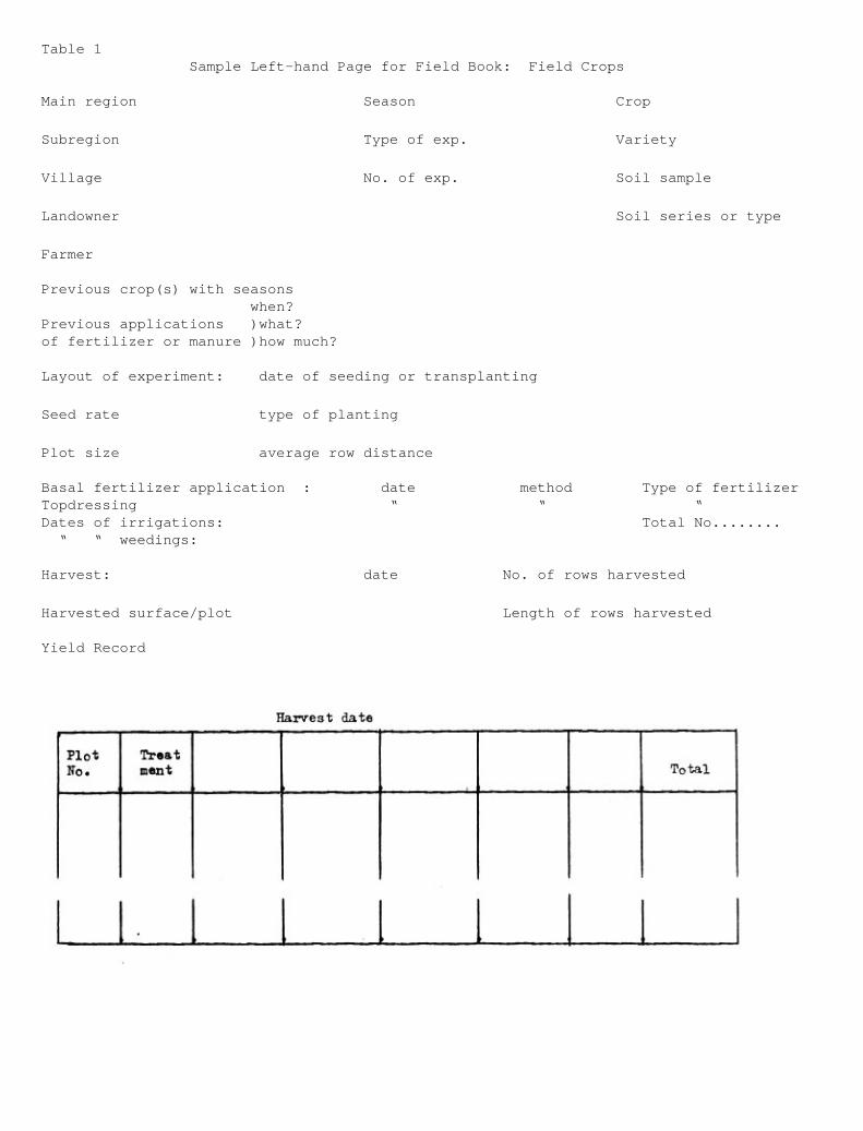
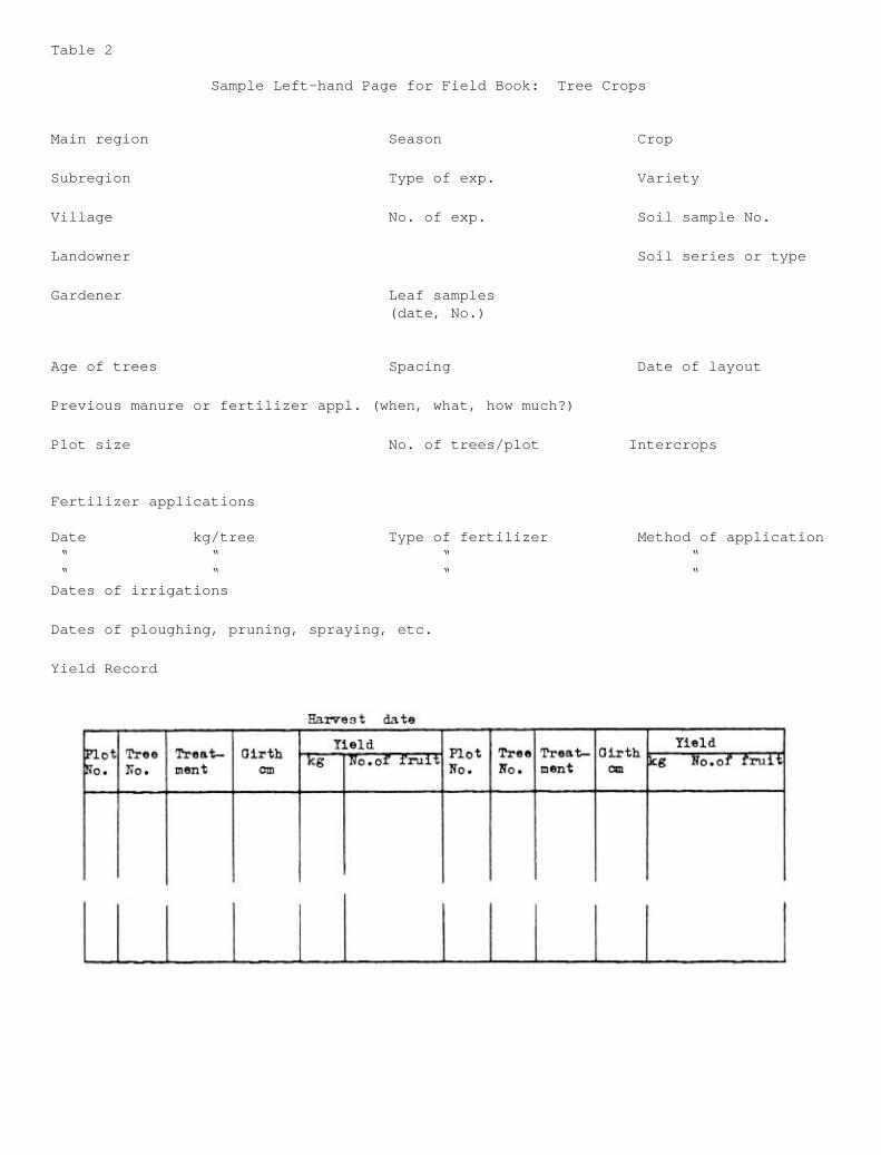
In the field book the two facing pages are always used for one trial; on theleft-hand page the necessary information on the trial is recorded, and the lower partof the page contains a table for recording the plot yields. The right-hand side isreserved for the sketch of the trial including landmarks. It shows the position,treatments and, in the case of irregular plots, the surface of each plot. The lowerpart of this page may be reserved for a small plot-scoring table.

The information on the field recorded on the left-hand page should be limitedto those facts which are needed for later interpretation of the results and whichcan be collected in the field. Examples of a suitable arrangement of this left-handpage for field crops as well as for tree crops are shown in Tables 1 and 2.

The information “soil type” may have to be adjusted to local needs; “soil series”and “soil phases” may have to be recorded.

The yield table for field crops can be used for various crops and trials. Thefirst column shows the plot number as noted in the trial sketch on the right-handside, and the order of figures is a result of the randomization of treatments,being different in every trial. The second column shows the treatments in systematicorder. The advantage of keeping the treatments always in the same order in the fieldbooks is that mistakes in copying yields are largely prevented.

The other columns can be used in varions ways. For instance in the case of cotton,the columns are need to enter the yields of successive pickings with the date of thepickings in the heading and with the total yield in the last column. For sugar beets,one column is used for the raw plot yield and the next column for entering test weightsof washed lots from which the percentage of earth is calculated. The last column willbe the corrected weights of clean beets. Similar usage can be made of the columnsfor other crops.

The yield table for tree crops is in two equal halves to save space but willneed an extension in most cases, since the items for each tree must be recorded sepa-rately.

Field data sheets

From the field book as a basic record, field data sheets are copied in duplicate or triplicate. They are designed in exactly the same way as the field book’s left-hand pages. These sheets are sent to project headquarters for compilation and evaluation of results. The sheets are first grouped into sets of experiments and from each group work sheets and summary tables are made as described under 4.2. Copied data must al- ways be checked carefully.

Harvea t date

Treatrcen t

PlotTotalNo .

Table 1 Sample Left-hand Page for Field Book: Field Crops

Main region Season Crop

Subregion Type of exp. Variety

Village No. of exp. Soil sample

Landowner Soil series or type

Farmer

Previous crop(s) with seasons when?Previous applications )what?of fertilizer or manure )how much?

Layout of experiment: date of seeding or transplanting

Seed rate type of planting

Plot size average row distance

Basal fertilizer application : date method Type of fertilizerTopdressing “ “ “Dates of irrigations: Total No........ “ “ weedings:

Harvest: date No. of rows harvested

Harvested surface/plot Length of rows harvested

Yield Record

Harve3t date

Plotr;o.

TreeNo.

,

Treatment

Girthcm

'field Pot-No.

TreeNo.

Treatment

Girthcm

Yieldkg 7go.of fruit kg No.of truit

Table 2

Sample Left-hand Page for Field Book: Tree Crops

Main region Season Crop

Subregion Type of exp. Variety

Village No. of exp. Soil sample No.

Landowner Soil series or type

Gardener Leaf samples (date, No.)

Age of trees Spacing Date of layout

Previous manure or fertilizer appl. (when, what, how much?)

Plot size No. of trees/plot Intercrops

Fertilizer applications

Date kg/tree Type of fertilizer Method of application “ “ “ “ “ “ “ “ Dates of irrigations

Dates of ploughing, pruning, spraying, etc.

Yield Record

3. Designs, Fertilizer Rates and Statistical Checks

3.1 Introduction

The planning of a set of trials on farmers’ fields consists of the choiceof a suitable experimental design and the choice of fertilizer rates. Comparedwith replicated complex experiments on fields of experimental stations, the planningof area-wide experiments on farmers’ fields is based on a wider range of practicalcriteria. The primary demand is of course that the experiment should give a clearanswer to the posed question. The fertilizer rates trial, for instance, shouldshow which kind and quantity of plant nutrient should be applied to a certain cropto achieve highest economic and physical gains. In addition to this primary needthe trials should give the desired answer in the shortest possible time; labourand costs should be kept at a reasonably low level; and results should have therequired degree of reliability for recommendations to farmers.

These additional needs, which obviously demand efficiency of operation, suggestthat simple, straightforward approaches are likely to give best results. Whilethe efficiency of operations is mainly dependent on the organization of the work,the requested reliability of results is closely related to the chosen experimentaldesign, i.e. the combination of treatments applied to each replicate, and experimentalfertilizer rates used.

With regard to the experimental design the primary requirement is the possibilityof calculating response curves or response surfaces, which are generally called“production functions”. If with a certain nutrient only one application rate weretested and we knew the yield increase due to this application, even with the higheststatistical precision we could not answer the question of whether there are otherrates that will give even higher returns, and what these rates are. (See also 3.3.1.1.)Therefore return curves calculated from at least three points, allowing estimationof the optimum rates, are needed for all major nutrient elements which are knownto affect the yield, or which are most likely to do so. Only in areas where it isknown that a certain nutrient is normally ineffective can a single rate of thisnutrient be used as a safeguard.

3.1.1 Statistical checks

The bases for statistical checks of experimental results is of course the analysis of variance. The variance relations show the experimenter the results in which he can have confidence and those which have to be checked further.

However, in this type of practical experiments one will encounter special cases which call for an open-minded approach in interpreting results rather than a strictly conventional one.

The magnitude of a response is of primary importance because large crop responses are likely to result in high economic benefits. If a crop response is very small but statistically highly significant, the treatment bringing about this response may not be interesting because its economic return is too low or negative. The high significance tells the experimenter that in repeating the trials he is likely to find the same low effect again.

The reverse often happens in trial sets with few replicates when high responses of even 30 percent or more of the check yield may be statistically insignificant. In such cases, obviously, the inference that there is no response or even that the response is too unreliable to be regarded is not allowed. In this case the prospect of getting a high and economically beneficial response is good and the experimenter should either refine his experimental technique or increase the number of trials, or both, in order to obtain more reliable results.

3.1.2 Significance levels

This leads to the matter of significance levels which is closely related to the standard error. It is fortunate that current thinking tends more and more to accept that the significance levels of 5 and 1 percent usually applied in experimental work are too arbitrary and sometimes unsatisfactory.

It is the type of risk and the magnitude of input and gain which decide the acceptability of chance. This may be illustrated by the following example: A farmer has a choice between a treatment repaying $5 for each dollar invested at a probability rate of 8 out of 10 (signi- ficance level of 20 percent), and another treatment requiring the same input which repays only $1.50 for each invested dollar at the probability rate of 19 out of 20, (significance level of 5 percent). There is little doubt that the average farmer will prefer the first treatment and will be doubtful about the second although it is “significant” and the first not, according to the usual 5 percent limit. This choice is perfectly right if we realize that the existence of a fertilizer effect is hardly in doubt and only its magnitude is in question.

Summarizing, it is seen that the statistica obtained by the variance analyses mainly help the experimenter to decide on the next step to be taken in the chain of investigations he is carrying out. Therefore, a basic variance analysis should be carried out for each set of trials.

The conventional significance levels of 5 and 1 percent, however, are of only relative value and are not to be taken as an absolute standard.

The production functions are essential for the evaluation of optimum fertilizer rates and as such contribute more to the ultimate decisions than single rate effects. Also regarding the production functions, the variance analysis will show the investigator which parts of his results need further experiments, while the shape of the functions and the magnitude of effects is a basis for making fertilizer recommendations.

Finally it should be said that in aiming at reliable return curves and surfaces the choice of fertilizer rates for the trials is of greatest importance. Experienced investigators know that well-chosen rates account for half the success. Therefore, the choice of rates is discussed first in the following section, to be followed by the choice of experimental designs.

3.2 Choice of fertilizer rates for trials on cultivators fields

3.2.1 General

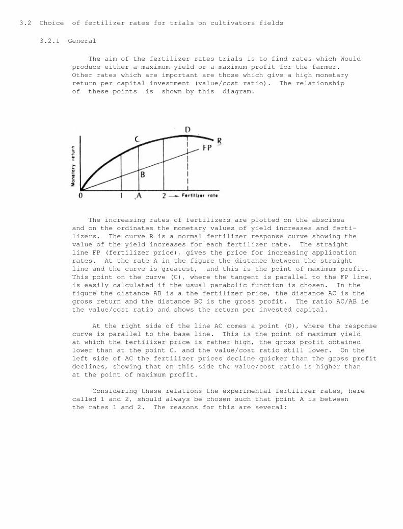
The aim of the fertilizer rates trials is to find rates which Would produce either a maximum yield or a maximum profit for the farmer. Other rates which are important are those which give a high monetary return per capital investment (value/cost ratio). The relationship of these points is shown by this diagram.

The increasing rates of fertilizers are plotted on the abscissa and on the ordinates the monetary values of yield increases and ferti- lizers. The curve R is a normal fertilizer response curve showing the value of the yield increases for each fertilizer rate. The straight line FP (fertilizer price), gives the price for increasing application rates. At the rate A in the figure the distance between the straight line and the curve is greatest, and this is the point of maximum profit. This point on the curve (C), where the tangent is parallel to the FP line, is easily calculated if the usual parabolic function is chosen. In the figure the distance AB is a the fertilizer price, the distance AC is the gross return and the distance BC is the gross profit. The ratio AC/AB ie the value/cost ratio and shows the return per invested capital.

At the right side of the line AC comes a point (D), where the response curve is parallel to the base line. This is the point of maximum yield at which the fertilizer price is rather high, the gross profit obtained lower than at the point C, and the value/cost ratio still lower. On the left side of AC the fertilizer prices decline quicker than the gross profit declines, showing that on this side the value/cost ratio is higher than at the point of maximum profit.

Considering these relations the experimental fertilizer rates, here called 1 and 2, should always be chosen such that point A is between the rates 1 and 2. The reasons for this are several:

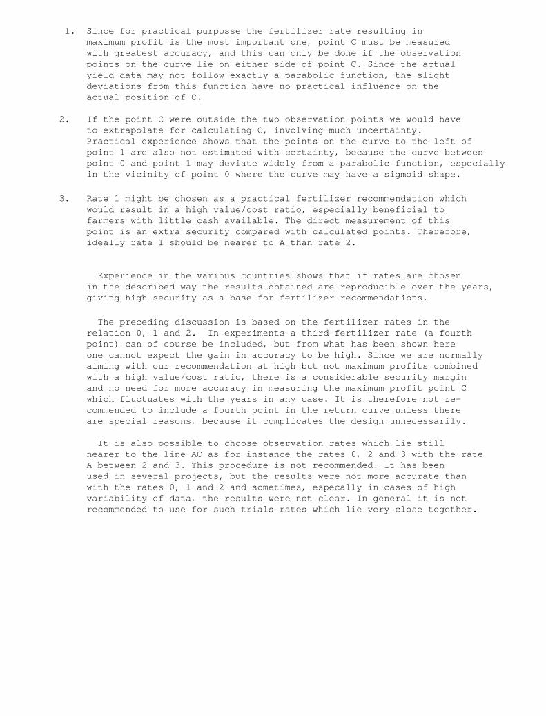
l. Since for practical purposse the fertilizer rate resulting in maximum profit is the most important one, point C must be measured with greatest accuracy, and this can only be done if the observation points on the curve lie on either side of point C. Since the actual yield data may not follow exactly a parabolic function, the slight deviations from this function have no practical influence on the actual position of C.

2. If the point C were outside the two observation points we would have to extrapolate for calculating C, involving much uncertainty. Practical experience shows that the points on the curve to the left of point 1 are also not estimated with certainty, because the curve between point 0 and point 1 may deviate widely from a parabolic function, especially in the vicinity of point 0 where the curve may have a sigmoid shape.

3. Rate 1 might be chosen as a practical fertilizer recommendation which would result in a high value/cost ratio, especially beneficial to farmers with little cash available. The direct measurement of this point is an extra security compared with calculated points. Therefore, ideally rate 1 should be nearer to A than rate 2.

Experience in the various countries shows that if rates are chosen in the described way the results obtained are reproducible over the years, giving high security as a base for fertilizer recommendations.

The preceding discussion is based on the fertilizer rates in the relation 0, 1 and 2. In experiments a third fertilizer rate (a fourth point) can of course be included, but from what has been shown here one cannot expect the gain in accuracy to be high. Since we are normally aiming with our recommendation at high but not maximum profits combined with a high value/cost ratio, there is a considerable security margin and no need for more accuracy in measuring the maximum profit point C which fluctuates with the years in any case. It is therefore not re- commended to include a fourth point in the return curve unless there are special reasons, because it complicates the design unnecessarily.

It is also possible to choose observation rates which lie still nearer to the line AC as for instance the rates 0, 2 and 3 with the rate A between 2 and 3. This procedure is not recommended. It has been used in several projects, but the results were not more accurate than with the rates 0, 1 and 2 and sometimes, especally in cases of high variability of data, the results were not clear. In general it is not recommended to use for such trials rates which lie very close together.

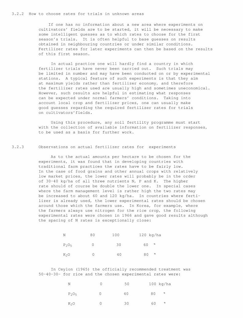
3.2.2 How to choose rates for trials in unknown areas

If one has no information about a new area where experiments on cultivators’ fields are to be started, it will be necessary to make some intelligent guesses as to which rates to choose for the first season’s trials. It is often helpful to base guesses on results obtained in neighbouring countries or under similar conditions. Fertilizer rates for later experiments can then be based on the results of this first season.

In actual practice one will hardly find a country in which fertilizer trials have never been carried out. Such trials may be limited in number and may have been conducted on or by experimental stations. A typical feature of such experiments is that they aim at maximum yields rather than fertilizer economy, and therefore the fertilizer rates used are usually high and sometimes uneconomical. However, such results are helpful in estimating what responses can be expected under normal farmers’ conditions. Taking into account local crop and fertilizer prices, one can usually make good guesses regarding the required fertilizer rates for trials on cultivators’fields.

Using this procedure, any soil fertility programme must start with the collection of available information on fertilizer responses, to be used as a basis for further work.

3.2.3 Observations on actual fertilizer rates for experiments

As to the actual amounts per hectare to be chosen for the experiments, it was found that in developing countries with traditional farm practices the rates have to be fairly low. In the case of food grains and other annual crops with relatively low market prices, the lower rates will probably be in the order of 30-40 kg/ha of all three nutrients N, P and K. The higher rate should of course be double the lower one. In special cases where the farm management level is rather high the two rates may be increased to about 60 and 120 kg/ha. In countries where ferti- lizer is already used, the lower experimental rates should be chosen around those which the farmers use. In Korea, for example, where the farmers always use nitrogen for the rice crop, the following experimental rates were chosen in 1966 and gave good results although the spacing of N rates is exceptionally close:

N 80 100 120 kg/ha

P 2O5 0 30 60 “

K 2O 0 40 80 “

In Ceylon (1965) the officially recommended treatment was 50-40-30- for rice and the chosen experimental rates were:

N 0 50 100 kg/ha

P 2O5 0 40 80 “

K 2O 0 30 60 “

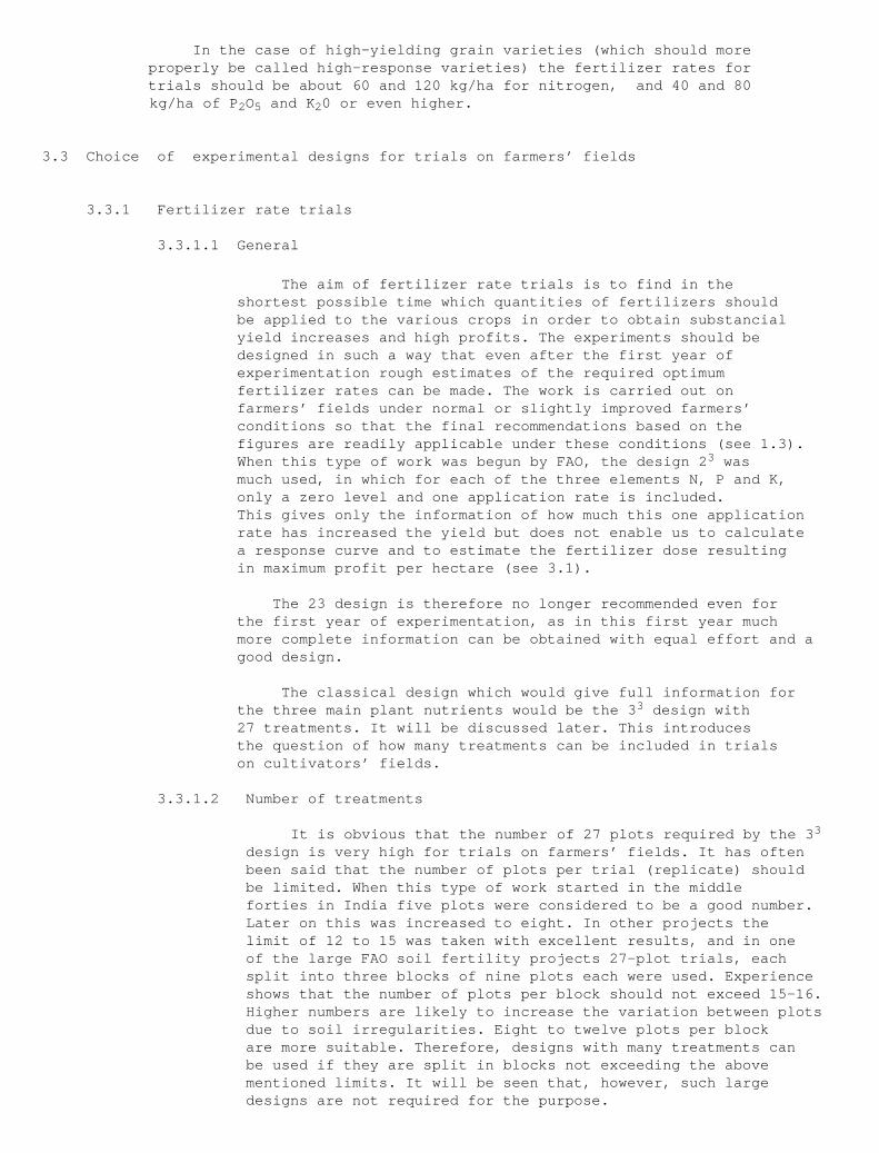
In the case of high-yielding grain varieties (which should more properly be called high-response varieties) the fertilizer rates for trials should be about 60 and 120 kg/ha for nitrogen, and 40 and 80 kg/ha of P 2O5 and K 20 or even higher.

3.3 Choice of experimental designs for trials on farmers’ fields

3.3.1 Fertilizer rate trials

3.3.1.1 General

The aim of fertilizer rate trials is to find in the shortest possible time which quantities of fertilizers should be applied to the various crops in order to obtain substancial yield increases and high profits. The experiments should be designed in such a way that even after the first year of experimentation rough estimates of the required optimum fertilizer rates can be made. The work is carried out on farmers’ fields under normal or slightly improved farmers’ conditions so that the final recommendations based on the figures are readily applicable under these conditions (see 1.3). When this type of work was begun by FAO, the design 2 3 was much used, in which for each of the three elements N, P and K, only a zero level and one application rate is included. This gives only the information of how much this one application rate has increased the yield but does not enable us to calculate a response curve and to estimate the fertilizer dose resulting in maximum profit per hectare (see 3.1).

The 23 design is therefore no longer recommended even for the first year of experimentation, as in this first year much more complete information can be obtained with equal effort and a good design.

The classical design which would give full information for the three main plant nutrients would be the 3 3 design with 27 treatments. It will be discussed later. This introduces the question of how many treatments can be included in trials on cultivators’ fields.

3.3.1.2 Number of treatments

It is obvious that the number of 27 plots required by the 3 3

design is very high for trials on farmers’ fields. It has often been said that the number of plots per trial (replicate) should be limited. When this type of work started in the middle forties in India five plots were considered to be a good number. Later on this was increased to eight. In other projects the limit of 12 to 15 was taken with excellent results, and in one of the large FAO soil fertility projects 27-plot trials, each split into three blocks of nine plots each were used. Experience shows that the number of plots per block should not exceed 15-16. Higher numbers are likely to increase the variation between plots due to soil irregularities. Eight to twelve plots per block are more suitable. Therefore, designs with many treatments can be used if they are split in blocks not exceeding the above mentioned limits. It will be seen that, however, such large designs are not required for the purpose.

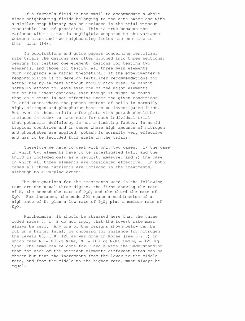
If a farmer’s field is too small to accommodate a wholeblock neighbouring fields belonging to the same owner and witha similar crop history can be included in the trial withoutmeasurable loss of precision. This is true because thevariance within sites is negligible compared to the variancebetween sites and two neighbouring fields are one site inthis case (14).

In publications and guide papers concerning fertilizerrate trials the designs are often grouped into three sections:designs for testing one element, designs for testing twoelements, and those for testing all three main elements.Such groupings are rather theoretical. If the experimenter’sresponsibility is to develop fertilizer recommendations foractual use by farmers without unduly high risk, he cannotnormally afford to leave even one of the major elementsout of his investigations, even though it might be foundthat an element is not effective under the given conditions.In arid zones where the potash content of soils is normallyhigh, nitrogen and phosphorus have to be investigated first.But even in these trials a few plots with potash should beincluded in order to make sure for each individual trialthat potassium deficiency is not a limiting factor. In humidtropical countries and in cases where high amounts of nitrogenand phosphates are applied, potash is normally very effectiveand has to be included full scale in the trials.

Therefore we have to deal with only two cases: 1) the casein which two elements have to be investigated fully and thethird is included only as a security measure, and 2) the casein which all three elements are considered effective. In bothcases all three nutrients are included in the treatments,although to a varying extent.

The designations for the treatments used in the followingtext are the usual three digits, the first showing the rateof N, the second the rate of P 2O5 and the third the rate ofK2O. For instance, the code 201 means a combination of ahigh rate of N, plus a low rate of P 2O5 plus a medium rate ofK2O.

Furthermore, it should be stressed here that the threecoded rates 0, 1, 2 do not imply that the lowest rate mustalways be zero. Any one of the designs shown below can beput on a higher level, by choosing for instance for nitrogenthe levels 80, 100, 120 as was done in Korea (see 3.2.3) inwhich case N 0 = 80 kg N/ha, N 1 = 100 kg N/ha and N 2 = 120 kgN/ha. The same can be done for P and K with the understandingthat for each of the nutrient elements different rates can bechosen but that the increments from the lower to the middlerate, and from the middle to the higher rate, must always beequal.

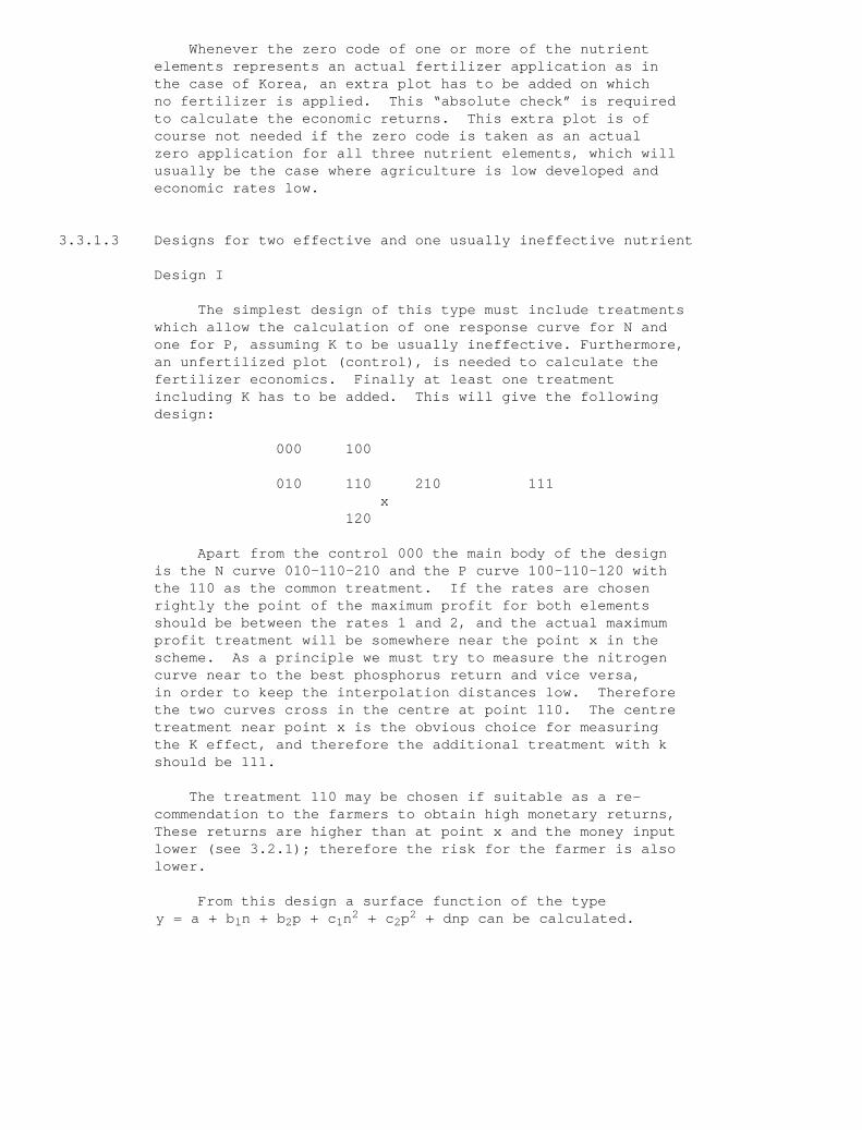
Whenever the zero code of one or more of the nutrient elements represents an actual fertilizer application as in the case of Korea, an extra plot has to be added on which no fertilizer is applied. This “absolute check” is required to calculate the economic returns. This extra plot is of course not needed if the zero code is taken as an actual zero application for all three nutrient elements, which will usually be the case where agriculture is low developed and economic rates low.

3.3.1.3 Designs for two effective and one usually ineffective nutrient

Design I

The simplest design of this type must include treatments which allow the calculation of one response curve for N and one for P, assuming K to be usually ineffective. Furthermore, an unfertilized plot (control), is needed to calculate the fertilizer economics. Finally at least one treatment including K has to be added. This will give the following design:

000 100

010 110 210 111 x 120

Apart from the control 000 the main body of the design is the N curve 010-110-210 and the P curve 100-110-120 with the 110 as the common treatment. If the rates are chosen rightly the point of the maximum profit for both elements should be between the rates 1 and 2, and the actual maximum profit treatment will be somewhere near the point x in the scheme. As a principle we must try to measure the nitrogen curve near to the best phosphorus return and vice versa, in order to keep the interpolation distances low. Therefore the two curves cross in the centre at point 110. The centre treatment near point x is the obvious choice for measuring the K effect, and therefore the additional treatment with k should be 111.

The treatment 110 may be chosen if suitable as a re- commendation to the farmers to obtain high monetary returns, These returns are higher than at point x and the money input lower (see 3.2.1); therefore the risk for the farmer is also lower.

From this design a surface function of the type y = a + b l n + b 2p + c 1n2 + c 2p2 + dnp can be calculated.

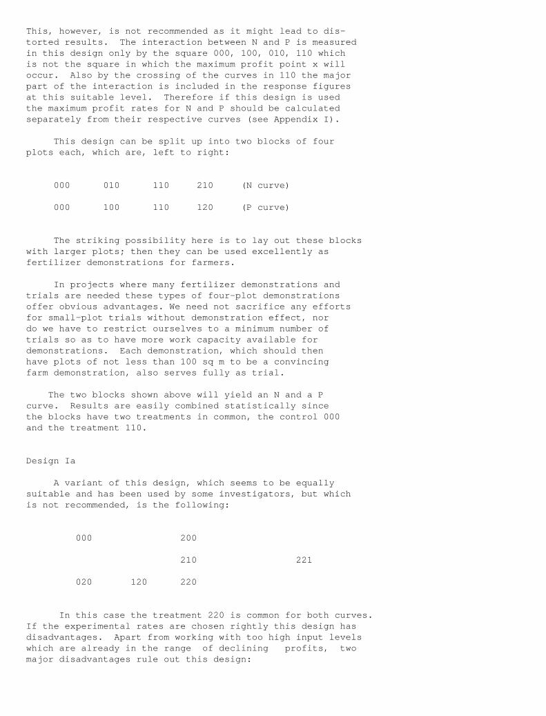
This, however, is not recommended as it might lead to dis-torted results. The interaction between N and P is measuredin this design only by the square 000, 100, 010, 110 whichis not the square in which the maximum profit point x willoccur. Also by the crossing of the curves in 110 the majorpart of the interaction is included in the response figuresat this suitable level. Therefore if this design is usedthe maximum profit rates for N and P should be calculatedseparately from their respective curves (see Appendix I).

This design can be split up into two blocks of fourplots each, which are, left to right:

000 010 110 210 (N curve)

000 100 110 120 (P curve)

The striking possibility here is to lay out these blockswith larger plots; then they can be used excellently asfertilizer demonstrations for farmers.

In projects where many fertilizer demonstrations andtrials are needed these types of four-plot demonstrationsoffer obvious advantages. We need not sacrifice any effortsfor small-plot trials without demonstration effect, nordo we have to restrict ourselves to a minimum number oftrials so as to have more work capacity available fordemonstrations. Each demonstration, which should thenhave plots of not less than 100 sq m to be a convincingfarm demonstration, also serves fully as trial.

The two blocks shown above will yield an N and a Pcurve. Results are easily combined statistically sincethe blocks have two treatments in common, the control 000and the treatment 110.

Design Ia

A variant of this design, which seems to be equallysuitable and has been used by some investigators, but whichis not recommended, is the following:

000 200

210 221

020 120 220

In this case the treatment 220 is common for both curves.If the experimental rates are chosen rightly this design hasdisadvantages. Apart from working with too high input levelswhich are already in the range of declining profits, twomajor disadvantages rule out this design:

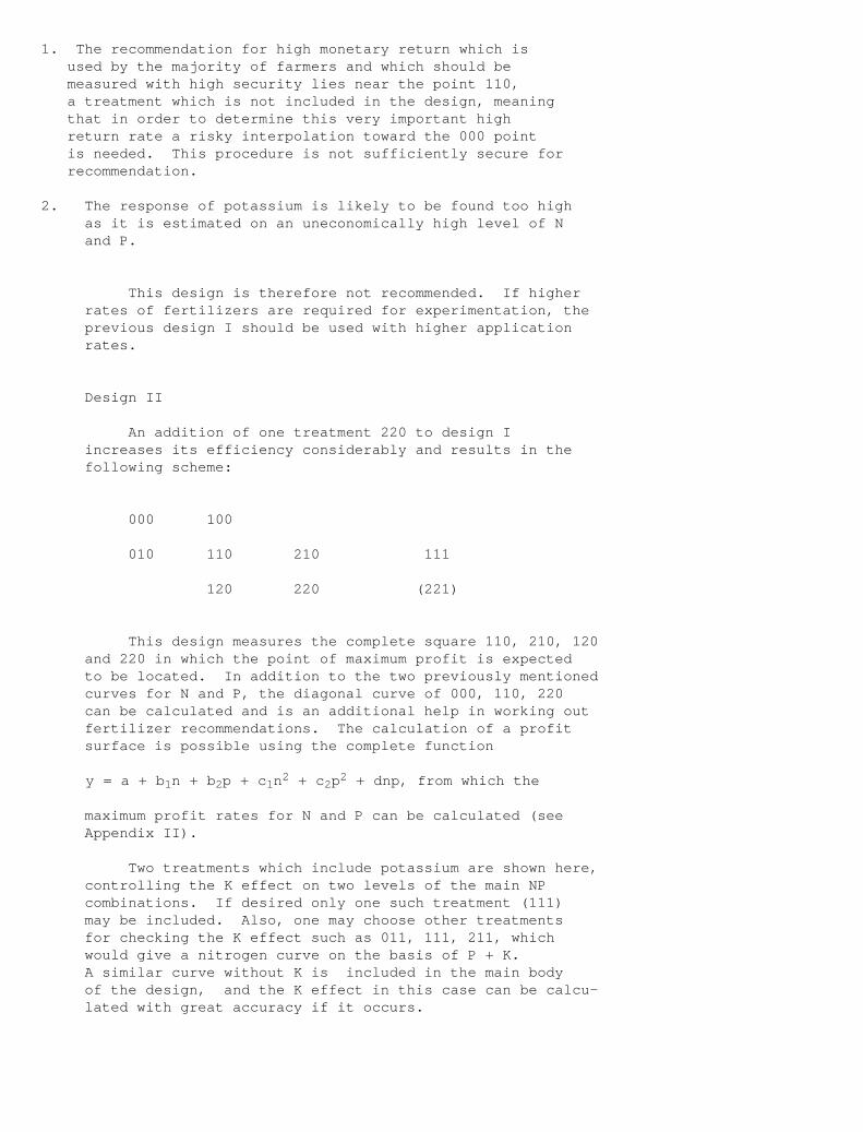
1. The recommendation for high monetary return which is used by the majority of farmers and which should be measured with high security lies near the point 110, a treatment which is not included in the design, meaning that in order to determine this very important high return rate a risky interpolation toward the 000 point is needed. This procedure is not sufficiently secure for recommendation.

2. The response of potassium is likely to be found too high as it is estimated on an uneconomically high level of N and P.

This design is therefore not recommended. If higher rates of fertilizers are required for experimentation, the previous design I should be used with higher application rates.

Design II

An addition of one treatment 220 to design I increases its efficiency considerably and results in the following scheme:

000 100

010 110 210 111

120 220 (221)

This design measures the complete square 110, 210, 120 and 220 in which the point of maximum profit is expected to be located. In addition to the two previously mentioned curves for N and P, the diagonal curve of 000, 110, 220 can be calculated and is an additional help in working out fertilizer recommendations. The calculation of a profit surface is possible using the complete function

y = a + b 1n + b 2p + c 1n2 + c 2p2 + dnp, from which the

maximum profit rates for N and P can be calculated (see Appendix II).

Two treatments which include potassium are shown here, controlling the K effect on two levels of the main NP combinations. If desired only one such treatment (111) may be included. Also, one may choose other treatments for checking the K effect such as 011, 111, 211, which would give a nitrogen curve on the basis of P + K. A similar curve without K is included in the main body of the design, and the K effect in this case can be calcu- lated with great accuracy if it occurs.

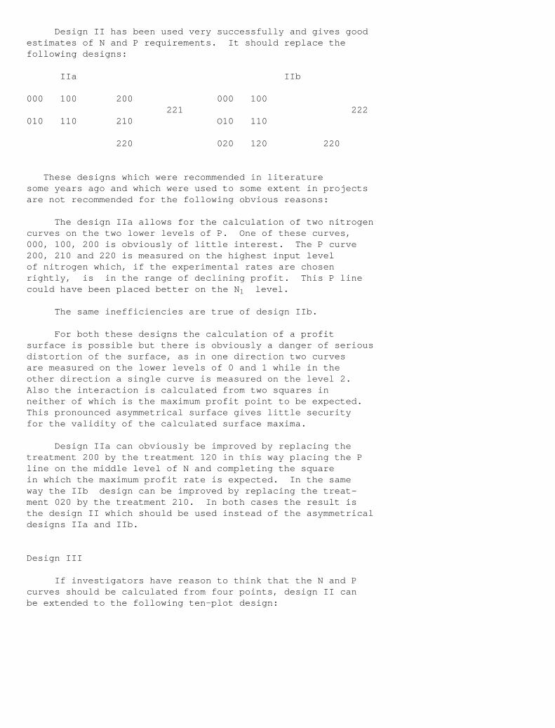
Design II has been used very successfully and gives goodestimates of N and P requirements. It should replace thefollowing designs:

IIa IIb

000 100 200 000 100 221 222010 110 210 O10 110

220 020 120 220

These designs which were recommended in literaturesome years ago and which were used to some extent in projectsare not recommended for the following obvious reasons:

The design IIa allows for the calculation of two nitrogencurves on the two lower levels of P. One of these curves,000, 100, 200 is obviously of little interest. The P curve200, 210 and 220 is measured on the highest input levelof nitrogen which, if the experimental rates are chosenrightly, is in the range of declining profit. This P linecould have been placed better on the N 1 level.

The same inefficiencies are true of design IIb.

For both these designs the calculation of a profitsurface is possible but there is obviously a danger of seriousdistortion of the surface, as in one direction two curvesare measured on the lower levels of 0 and 1 while in theother direction a single curve is measured on the level 2.Also the interaction is calculated from two squares inneither of which is the maximum profit point to be expected.This pronounced asymmetrical surface gives little securityfor the validity of the calculated surface maxima.

Design IIa can obviously be improved by replacing thetreatment 200 by the treatment 120 in this way placing the Pline on the middle level of N and completing the squarein which the maximum profit rate is expected. In the sameway the IIb design can be improved by replacing the treat-ment 020 by the treatment 210. In both cases the result isthe design II which should be used instead of the asymmetricaldesigns IIa and IIb.

Design III

If investigators have reason to think that the N and Pcurves should be calculated from four points, design II canbe extended to the following ten-plot design:

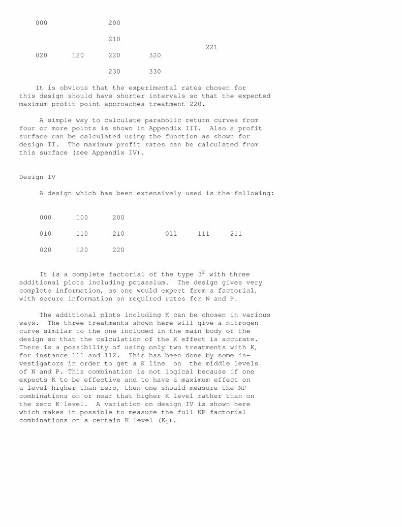
000 200

210 221 020 120 220 320

230 330

It is obvious that the experimental rates chosen forthis design should have shorter intervals so that the expectedmaximum profit point approaches treatment 220.

A simple way to calculate parabolic return curves fromfour or more points is shown in Appendix III. Also a profitsurface can be calculated using the function as shown fordesign II. The maximum profit rates can be calculated fromthis surface (see Appendix IV).

Design IV

A design which has been extensively used is the following:

000 100 200

010 110 210 0ll 111 211

020 120 220

It is a complete factorial of the type 3 2 with threeadditional plots including potassium. The design gives verycomplete information, as one would expect from a factorial,with secure information on required rates for N and P.

The additional plots including K can be chosen in variousways. The three treatments shown here will give a nitrogencurve similar to the one included in the main body of thedesign so that the calculation of the K effect is accurate.There is a possibility of using only two treatments with K,for instance 111 and 112. This has been done by some in-vestigators in order to get a K line on the middle levelsof N and P. This combination is not logical because if oneexpects K to be effective and to have a maximum effect ona level higher than zero, then one should measure the NPcombinations on or near that higher K level rather than onthe zero K level. A variation on design IV is shown herewhich makes it possible to measure the full NP factorialcombinations on a certain K level (K 1).

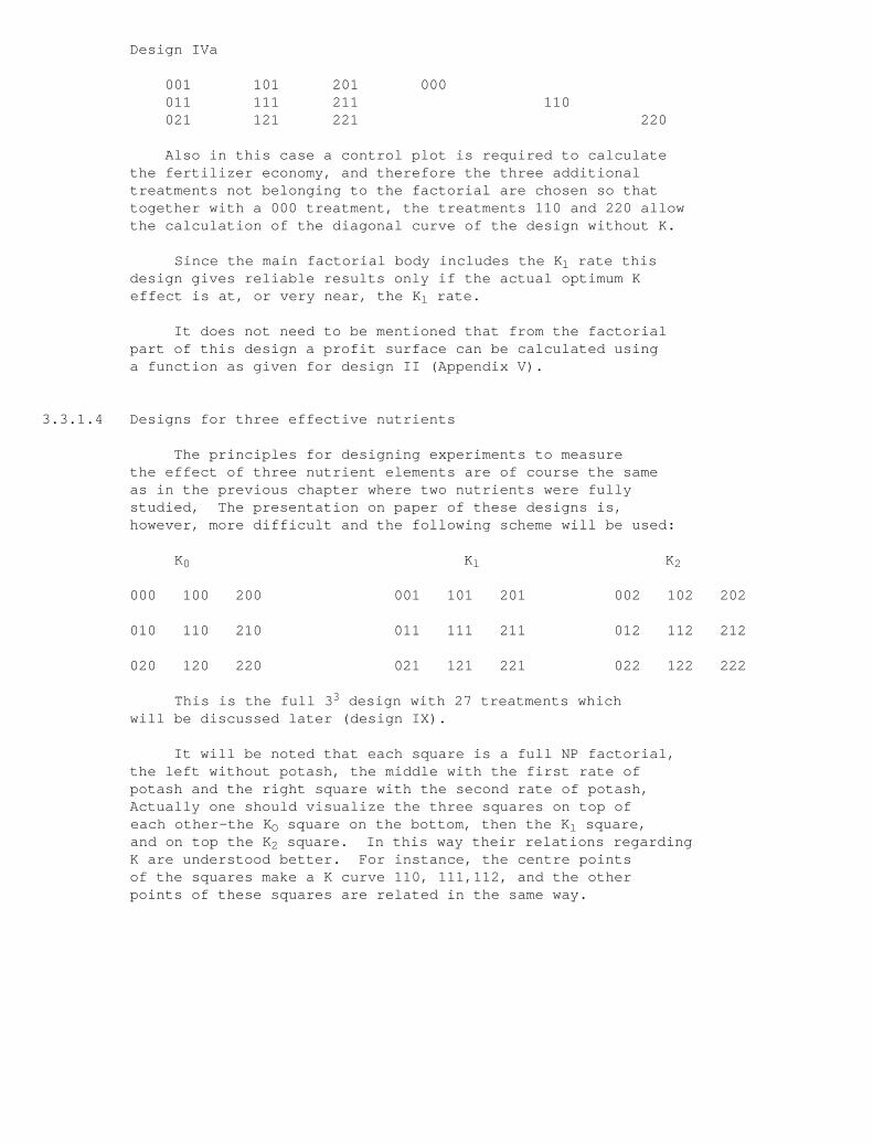
Design IVa

001 101 201 000 011 111 211 110 021 121 221 220

Also in this case a control plot is required to calculate the fertilizer economy, and therefore the three additional treatments not belonging to the factorial are chosen so that together with a 000 treatment, the treatments 110 and 220 allow the calculation of the diagonal curve of the design without K.

Since the main factorial body includes the K l rate this design gives reliable results only if the actual optimum K effect is at, or very near, the K l rate.

It does not need to be mentioned that from the factorial part of this design a profit surface can be calculated using a function as given for design II (Appendix V).

3.3.1.4 Designs for three effective nutrients

The principles for designing experiments to measure the effect of three nutrient elements are of course the same as in the previous chapter where two nutrients were fully studied, The presentation on paper of these designs is, however, more difficult and the following scheme will be used:

K 0 K l K 2

000 100 200 001 101 201 002 102 202

010 110 210 011 111 211 012 112 212

020 120 220 021 121 221 022 122 222

This is the full 3 3 design with 27 treatments which will be discussed later (design IX).

It will be noted that each square is a full NP factorial, the left without potash, the middle with the first rate of potash and the right square with the second rate of potash, Actually one should visualize the three squares on top of each other-the K O square on the bottom, then the K l square, and on top the K 2 square. In this way their relations regarding K are understood better. For instance, the centre points of the squares make a K curve 110, 111,112, and the other points of these squares are related in the same way.

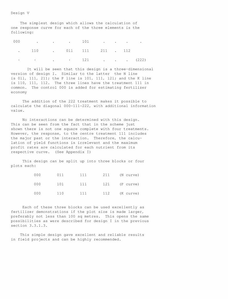
Design V

The simplest design which allows the calculation ofone response curve for each of the three elements is thefollowing:

000 . . . 101 . . . .

. 110 . 0ll 111 211 . 112

· · . · 121 . . . (222)

It will be seen that this design is a three-dimensionalversion of design I. Similar to the latter the N lineis 0ll, 111, 211; the P line is 101, 111, l2l; and the K lineis 110, 111, 112. The three lines have the treatment 111 incommon. The control 000 is added for estimating fertilizereconomy

The addition of the 222 treatment makes it possible tocalculate the diagonal 000-111-222, with additional informationvalue.

No interactions can be determined with this design.This can be seen from the fact that in the scheme justshown there is not one square complete with four treatments.However, the response, to the centre treatment 111 includesthe major past or the interaction. Therefore, the calcu-lation of yield functions is irrelevant and the maximumprofit rates are calculated for each nutrient from itsrespective curve. (See Appendix I)

This design can be split up into three blocks or fourplots each:

000 011 111 211 (N curve)

000 101 111 121 (P curve)

000 110 111 112 (K curve)

Each of these three blocks can be used excellently asfertilizer demonstrations if the plot size is made larger,preferably not less than 100 sq metres. This opens the samepossibilities as were described for design I in the previoussection 3.3.1.3.

This simple design gave excellent and reliable resultsin field projects and can be highly recommended.

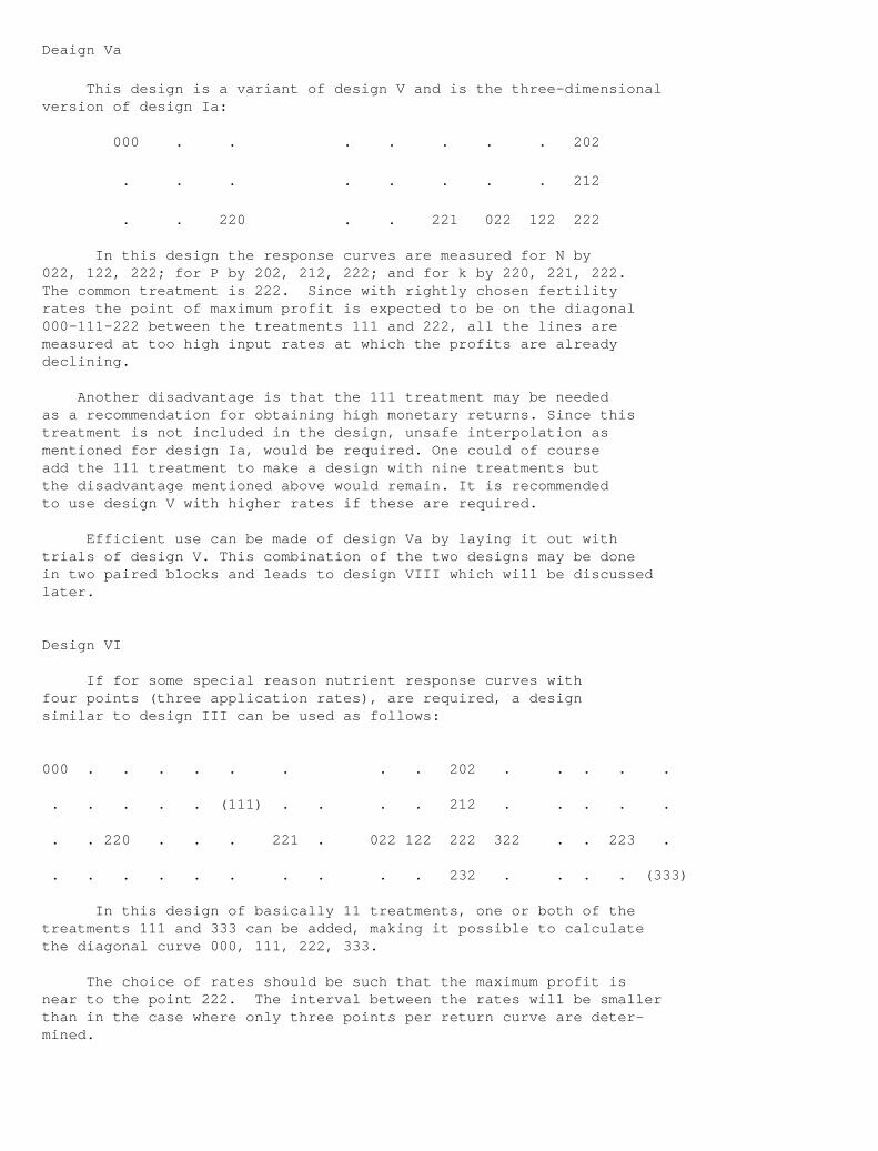
Deaign Va

This design is a variant of design V and is the three-dimensionalversion of design Ia:

000 . . . . . . . 202

. . . . . . . . 212

. . 220 . . 221 022 122 222

In this design the response curves are measured for N by022, 122, 222; for P by 202, 212, 222; and for k by 220, 221, 222.The common treatment is 222. Since with rightly chosen fertilityrates the point of maximum profit is expected to be on the diagonal000-111-222 between the treatments 111 and 222, all the lines aremeasured at too high input rates at which the profits are alreadydeclining.

Another disadvantage is that the 111 treatment may be neededas a recommendation for obtaining high monetary returns. Since thistreatment is not included in the design, unsafe interpolation asmentioned for design Ia, would be required. One could of courseadd the 111 treatment to make a design with nine treatments butthe disadvantage mentioned above would remain. It is recommendedto use design V with higher rates if these are required.

Efficient use can be made of design Va by laying it out withtrials of design V. This combination of the two designs may be donein two paired blocks and leads to design VIII which will be discussedlater.

Design VI

If for some special reason nutrient response curves withfour points (three application rates), are required, a designsimilar to design III can be used as follows:

000 . . . . . . . . 202 . . . . .

. . . . . (111) . . . . 212 . . . . .

. . 220 . . . 221 . 022 122 222 322 . . 223 .

. . . . . . . . . . 232 . . . . (333)

In this design of basically 11 treatments, one or both of thetreatments 111 and 333 can be added, making it possible to calculatethe diagonal curve 000, 111, 222, 333.

The choice of rates should be such that the maximum profit isnear to the point 222. The interval between the rates will be smallerthan in the case where only three points per return curve are deter-mined.

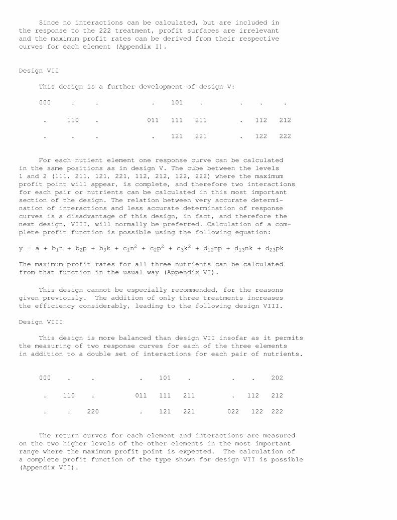
Since no interactions can be calculated, but are included inthe response to the 222 treatment, profit surfaces are irrelevantand the maximum profit rates can be derived from their respectivecurves for each element (Appendix I).

Design VII

This design is a further development of design V:

000 . . . 101 . . . .

. 110 . 011 111 211 . 112 212

. . . . 121 221 . 122 222

For each nutient element one response curve can be calculatedin the same positions as in design V. The cube between the levels1 and 2 (111, 211, 121, 221, 112, 212, 122, 222) where the maximumprofit point will appear, is complete, and therefore two interactionsfor each pair or nutrients can be calculated in this most importantsection of the design. The relation between very accurate determi-nation of interactions and less accurate determination of responsecurves is a disadvantage of this design, in fact, and therefore thenext design, VIII, will normally be preferred. Calculation of a com-plete profit function is possible using the following equation:

y = a + b l n + b 2p + b 3k + c l n2 + c 2p2 + c 3k2 + d l2 np + d l3 nk + d 23pk

The maximum profit rates for all three nutrients can be calculatedfrom that function in the usual way (Appendix VI).

This design cannot be especially recommended, for the reasonsgiven previously. The addition of only three treatments increasesthe efficiency considerably, leading to the following design VIII.

Design VIII

This design is more balanced than design VII insofar as it permitsthe measuring of two response curves for each of the three elementsin addition to a double set of interactions for each pair of nutrients.

000 . . . 101 . . . 202

. 110 . 0ll 111 211 . 112 212

. . 220 . 121 221 022 122 222

The return curves for each element and interactions are measuredon the two higher levels of the other elements in the most importantrange where the maximum profit point is expected. The calculation ofa complete profit function of the type shown for design VII is possible(Appendix VII).

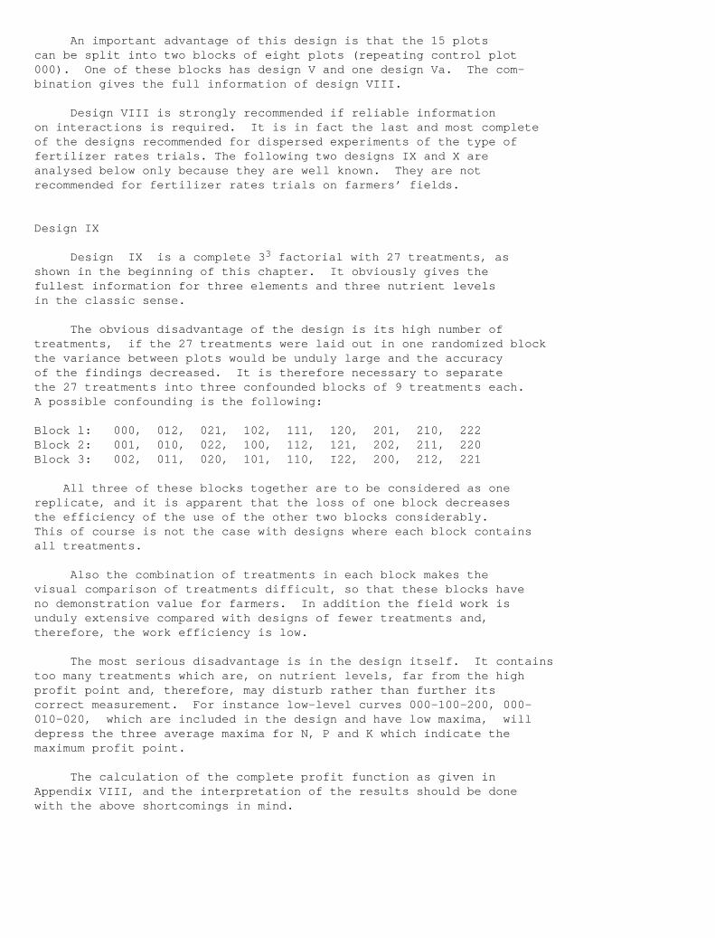
An important advantage of this design is that the 15 plotscan be split into two blocks of eight plots (repeating control plot000). One of these blocks has design V and one design Va. The com-bination gives the full information of design VIII.

Design VIII is strongly recommended if reliable informationon interactions is required. It is in fact the last and most completeof the designs recommended for dispersed experiments of the type offertilizer rates trials. The following two designs IX and X areanalysed below only because they are well known. They are notrecommended for fertilizer rates trials on farmers’ fields.

Design IX

Design IX is a complete 3 3 factorial with 27 treatments, asshown in the beginning of this chapter. It obviously gives thefullest information for three elements and three nutrient levelsin the classic sense.

The obvious disadvantage of the design is its high number oftreatments, if the 27 treatments were laid out in one randomized blockthe variance between plots would be unduly large and the accuracyof the findings decreased. It is therefore necessary to separatethe 27 treatments into three confounded blocks of 9 treatments each.A possible confounding is the following:

Block l: 000, 012, 021, 102, 111, 120, 201, 210, 222Block 2: 001, 010, 022, 100, 112, 121, 202, 211, 220Block 3: 002, 011, 020, 101, 110, I22, 200, 212, 221

All three of these blocks together are to be considered as onereplicate, and it is apparent that the loss of one block decreasesthe efficiency of the use of the other two blocks considerably.This of course is not the case with designs where each block containsall treatments.

Also the combination of treatments in each block makes thevisual comparison of treatments difficult, so that these blocks haveno demonstration value for farmers. In addition the field work isunduly extensive compared with designs of fewer treatments and,therefore, the work efficiency is low.

The most serious disadvantage is in the design itself. It containstoo many treatments which are, on nutrient levels, far from the highprofit point and, therefore, may disturb rather than further itscorrect measurement. For instance low-level curves 000-100-200, 000-010-020, which are included in the design and have low maxima, willdepress the three average maxima for N, P and K which indicate themaximum profit point.

The calculation of the complete profit function as given inAppendix VIII, and the interpretation of the results should be donewith the above shortcomings in mind.

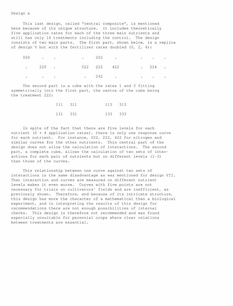
Design x

This last design, called “central composite”, is mentionedhere because of its unique structure. It includes theoreticallyfive application rates for each of the three main nutrients andstill has only 16 treatments including the control. The designconsists of two main parts. The first part, shown below, is a replicaof design V but with the fertilizer rates doubled (0, 2, 4):

000 . . . 202 . . . .

. 220 . 022 222 422 . 224 .

. . . . 242 . . . .

The second part is a cube with the rates 1 and 3 fittingsymmetrically into the first part, the centre of the cube beingthe treatment 222:

111 311 113 313

131 331 133 333

In spite of the fact that there are five levels for eachnutrient (0 + 4 application rates), there is only one response curvefor each nutrient. For instance, 022, 222, 422 for nitrogen andsimilar curves for the other nutrients. This central part of thedesign does not allow the calculation of interactions. The secondpart, a complete cube, allows the calculation of two sets of inter-actions for each pair of nutrients but on different levels (1-3)than those of the curves.

This relationship between one curve against two sets ofinteractions is the same disadvantage as was mentioned for design VII.That interaction and curves are measured on different nutrientlevels makes it even worse. Curves with five points are notnecessary for trials on cultivators’ fields and are inefficient, aspreviously shown. Therefore, and because of its intricate structure,this design has more the character of a mathematical than a biologicalexperiment, and in interpreting the results of this design forrecommendations there are not enough possibilities of internalchecks. This design is therefore not recommended and was foundespecially unsuitable for perennial crops where clear relationsbetween treatments are essential.

3.3.1.5 The problem of the fourth element

It will happen over and over again that experimental plants show deficiency sumptones which have nothing to do with the supply of the three major elements but are caused by the lack of a fourth element, which might be magnesium or sulfur or one of the trace elements. In such cases it is necessary to check on the practical importance of this deficiency by including this element in the experiment. It would be a mistake in this case to choose a design which is equally sensitive for the three major and the fourth elements. As a rule, the fourth element will not have as big an influence on the yield as the three major elements, and therefore the experiment should be more sensitive, for this fourth element than it is for the three major elements.

The most practical solution in this case is to keep the basic fertilizer rate design originally chosen for the three major elements or a simplified version of it but to increase the size of plots somewhat and separate each plot into two parts, one with and one without the fourth element. Randomization should decide for each plot which half receives the extra treatment and which not. In such a split-plot design the sensitivity for the three major elements is unchanged, while that for the fourth element is considerably higher. Practically speaking, one such replicate consists of two trials, one with and one without the fourth element.

Usually this type of trial is carried out with a few replicates only, in order to see whether the observed symptoms are due to the lack of the fourth element or not. One may even test more than one element in this way if they are likely to cause the symptoms.

The great advantages of the split-plot design are:

l. Nothing needs to be changed in the project routine except the extra treatments for a few of the replicates.

2. From each such trial also an untreated set of yield data is obtained, contributing as a normal replicate to the area average.

The information on the additionally tested elements is therefore obtained with minimum effort but high accuracy, which otherwise could only be achieved by elaborate special experiments.

A simplified version of the split-plot design is the following: Instead of randomizing for each plot which half gets the extra treatment, one can apply this treatmant to a whole row of plots in one strip, as shown in the diagram.

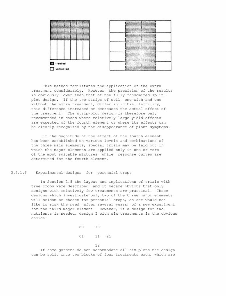
MI ',totedEJ untr.0,,d

This method facilitates the application of the extra treatment considerably. However, the precision of the results is obviously lower than that of the fully randomized split- plot design. If the two strips of soil, one with and one without the extra treatment, differ in initial fertility, this difference increases or decreases the actual effect of the treatment. The strip-plot design is therefore only recommended in cases where relatively large yield effects are expected of the fourth element or where its effects can be clearly recognized by the disappearance of plant symptoms.

If the magnitude of the effect of the fourth element has been established on various levels and combinations of the three main elements, special trials may be laid out in which the major elements are applied only in one or more of the most suitable mixtures, while response curves are determined for the fourth element.

3.3.1.6 Experimental designs for perennial crops

In Section 2.8 the layout and implications of trials with tree crops were described, and it became obvious that only designs with relatively few treatments are practical. Those designs which investigate only two of the three major elements will seldom be chosen for perennial crops, as one would not like to risk the need, after several years, of a new experiment for the third major element. However, if a design for two nutrients is needed, design I with six treatments is the obvious choice:

00 10

0l 11 21

12 If some gardens do not accommodate all six plots the design can be split into two blocks of four treatments each, which are

For the investigation of all three major elements design V (see 3.3.1.4) with eight treatments is recommended:

000 011 211

101 111 121

110 112

This design can be split into three blocks of four treat- ments each: 000, 011, 111, 211; 000, 101, 111, 121; 000, 110, 111, 112 resulting in the N, P and K curves respect- ively and having the control plot and the treatment 111 in common (See 3.3.1.4).

Interactions cannot be calculated with these designs, but the main part of the interaction is included in the effect of the treatment 111. See also design V.

3.3.2 Nutrient carrier comparison

A common need in fertilizer experiments is to compare the effects of various nitrogenous, phosphatic or potassic materials. In this comparison the differences found between the effects, for example, of urea and ammonium sulfate on the yields are often very small, and it is therefore advisable to carry out such comparisons also in exact experiments under controlled conditions in experiment stations, as pre- viously stated.

However, it is also necessary to compare these materials under normal farming conditions where obtained yields are lower and the effects perhaps different. The simple trials on farmers’ fields allow each of these materials to be evaluated economically on an area-wide basis. This knowledge is required by governments in order to arrive at technically sound fertilizer policies.

An efficient design for comparing different fertilizer materials is shown here. It consists of a control plot 000 and, if nitrogenous materials are compared, of a second plot fertilized with P alone or P + K, depending on the requirements of the soil. Each of the nitro- genous materials to be tested is applied in two different rates, together with the basic PK treatment. This results in the following design:

000

PK

U l PK lower rate of urea

U 2PK higher rate of urea

AS l PK lower rate of ammonium sulfate

AS 2PK higher rate of ammonium sulfate

The number of plots, which is six in the above case and eight when three different N materials are compared, is practical for work on cultivators’ fields.

For comparison of the effects of phosphatic or potassic materials the basic treatment will be NK or NP respectively.

The advantage of this design is that for each material a response curve can be calculated which results in an efficient comparison of the individual effects of the materials. The economy dependent partly on the price of the materials, is calculated in the same way as in the case of fertilizer rate trials.

3.3.3 Other trials with fertilizers

There are of course many other types of trials besides the ones that have been mentioned. A few practical suggestions for these are discussed in this section.

3.3.3.1 Time of application trials

In these trials the problem is often to choose between a single application of nitrogen at planting time and split application. P and K are usually applied at planting time. Since the difference in yield between single and split appli- cations of nitrogen is often rather small, the use of a split- plot design is recommended. It is convenient for this purpose to use the same standard fertilizer-rate design as used in the project and to increase the plot size sufficiently to be able to split each plot into two halves, of which one half receives the nitrogen at seeding time and the other as a split application.

3.3.3.2 Residual and cumulative fertilizer effects

The residual and cumulative effects of the various plant nutrients are very different but strongly interrelated. It is therefore necessary to estimate them with fairly complete designs of the types IV or VIII in which various rates and combinations of nutrients are included. It is then possible to measure the yield increases caused by residual fertilizer effects and calculate directly these effects and their interactions. In a second set of such trials cumulative fertilizer effects can be studied in the same way.

In general it might be said about residual effects that they are mainly important for certain simple rotations as found in many countries where normally a high-value cash crop, amply fertilized, is rotated with a crop of food grain of relatively low market value. The lower-value crop represents an excellent way to use the residual effects from the fertilizers applied to the cash crop but often will need some extra nitrogen.

3.3.3.3 Trials comparing placement of fertilizer with broadcasting

Also in this type of experiment a split-plot design is recommended, using as a basis one of the fertilizer rate designs applied in the project. The split-plot design will have the advantage that small differences in the effects between placement and broadcasting will be found.

3.3.3.4 Combined fertilizer variety trials

Usually only one or two selected highly suitable varieties are tested on a larger scale against local varieties or against a standard variety. These trials are made in the last phase of variety tests when their performances with regard to fertilizer use and economy are determined on farmer’s fields.

Such trials will not be started until fertilizer a responses are known at least roughly and preliminary fertilizer recommen- dations are available. In practice, therefore, these trials are relatively simple to plan and will vary according to available knowledge and needs. Some examples may illustrate this:

l. In an area where fertilizer rate trials are still being laid out in the second or third season and where local or older improved varieties are being used by the farmers, a highly promising variety is to be tested. In this case a second block with the new variety is laid out on selected sites in addition to the block which is used for the fertilizer rate determination. This paired block system is statistically not as accurate a com- parison as a split-plot design, but for practical purposes it is satisfactory for the comparison of varieties under farmers, conditions and it is much easier to lay out and harvest. A variant of the paired block design was described in 3.3.1.5 for the testing of a fourth element. Instead of the fourth element the new variety is sown in strips perpendicular to the length of the plots. Both the strips and the treatments are randomized.

2. If more than one new variety is to be tested against a local or standard variety the layout of three blocks on the site is not practical, mainly because it will not be possible to lay out sufficient replications with the given manpower and facilities. In this case the strip-plot variant described in (1.) above is used. The narrow plots are made longer in order to accommodate three or even more strips one for each variety. Randomization is done in the same way.

3. If fertilizer recommendations are already available, one can cut down the number of fertilizer treatments by using only the most promising nutrient combinations. If, for instance, in the case of wheat the recommendation for the standard variety is 50-40-0 the treatments for the ex- periments could be chosen as follows: 0-0-0 50-40-0 l00-80-0 50-40-30, or 0-0-0 50-40-0 100-40-0 50-80-0 100-80-0 and 50-40-30. Both sets of treatments include the 0-0-0 plot. Not only is this needed for the calculation of fertilizer economy but it is also most important to know the behaviour of the new variety on unfertilized fields.

In addition to this control plot the first treatment set includes the recommended rate 50-40-0 and the double rate allowing for the calculation of a response curve for each variety. This will allow a highly accurate comparison of the varieties. The last treatment is included as a safeguard in order to know from each site whether potassium was effective. In the second set of treatments the combinations 100-40-0 and 50-80-0 are added in order to obtain information on the varieties’ indi- vidual preferences for high N or high P application.

If to these six treatments 50-0-0 and 0-40-0 are added, one arrives at design I (see 3.3.1.3), which is also excellent- ly suitable for variety comparison. It allows the calculation of an N curve and a P curve in addition to a diagonal curve for each variety.

It should be stressed here that for high-yielding varieties with high fertilizer requirements one should take care to make the rates for these trials high enough, (see 3.2.2).

3.3.4 Some remarks on designs

For projects operating for several years it is a great advantage to use only one or two fertilizer rate designs throughout the whole project. If one wishes to start the work with a simpler design and continue later with a more complete one, the designs should be chosen such that the core is the same and one is only an extension of the other as has been shown in sections 3.3.1.3 and 3.3.1.4. In these sections it was also explained which of the variants are least efficient.

Also for certain types of trials other than fertilizer rate trials the basic designs should be used as described above. This maximum uniformity involving a minimum number of designs for the project has the invaluable advantage that the results from all crops and all seasons can be directly compared and that large area-samples are obtained (see 3.3.1.5).

Combining results of two essentially different designs mathema- tically involves adjustments of yield figures and responses, and these figures are never as reliable as directly measured ones. Therefore one should avoid such combinations if direct designs are available. For instance, the use of the asymmetric designs IIa and IIb separately and then combining them mathematically is inferior to using design II or IV. However, if conditions strictly exclude designs with more than a certain number of treatments as is the case with tree trials, even a simple efficient design may have to be split up into smaller blocks as shown under 3.3.1.6. Even in these cases, the most efficient practice is to keep the chosen design for all tree crops throughout the project.

4. Presentation and Interpretation of Results

4.1 General

The data obtained from the dispersed experiments on cultivators’ fields are verydifferent in nature from those of experiments under strictly controlled conditions.The fields of the experimental stations are usually uniform and so is their treatment,irrigation, etc. In such experiments the variance between plots is very small, andthe variance between fertilizer rates is normally greater than the variance betweenreplications.

In dispersed experiments the replicates (trials) are spread over large areas.Each replicate is on another field which belongs to another farmer. The soils ofall these fields vary, and there are other types of variations among fields all ofwhich together are characteristic of the area in question. The variance betweenthese replicates is much greater than on experimental stations, and it is a generalfeature that in the variance analysis the variance between trial sites is larger thanthat between treatments. This is itself is a hard test for the superiority of anyfertilizer combination which finally is selected for use.

The great advantage of this system is of course that the resulting figures arearea-wide averages, and the variance between the sites of the replicates is a directmeasure of the uniformity of the area. All these trials together form a “sample” ofthe area in a statistical sense. Therefore, if a treatment is found to be superiorwith a high significance-or more correctly, with a high probability rate-this pro-bability refers to the whole of the area including all farmers and conditions andprovides a measure of security for recommendations which could never be obtainedfrom one or two sites only even with the most exact experiments.

In this practical approach, highest precision is of little avail consideringthe variation within an area. It is the general validity of results which providesa safe basis for economically sound fertilizer recommendations. For the interpre-tation of results these facts should be kept clearly in mind.

The basic results from the trials are the average yields of each treatment,the so-called “treatment means”. To obtain them in a systematic and practical wayone may proceed as described in the following pages.

4.2 Work sheets and summary tables of results

When the field data sheets come in from the field (see 2.11), the yield dataare compiled on large work sheets for which standard account sheets can be used.Usually in the left-hand column the name of the village and the trial number isentered. Each row of the table refers to one trial (replicate). Each of thefollowing columns refers to one treatment. The yields are entered here. Afterthe last treatment column, column “sum” is carried, where the sum of all treatmentyields per trial is entered. This is later used for the calculation of the analysisof variance. Further to the right, columns for results of chemical soil analysesmay follow.

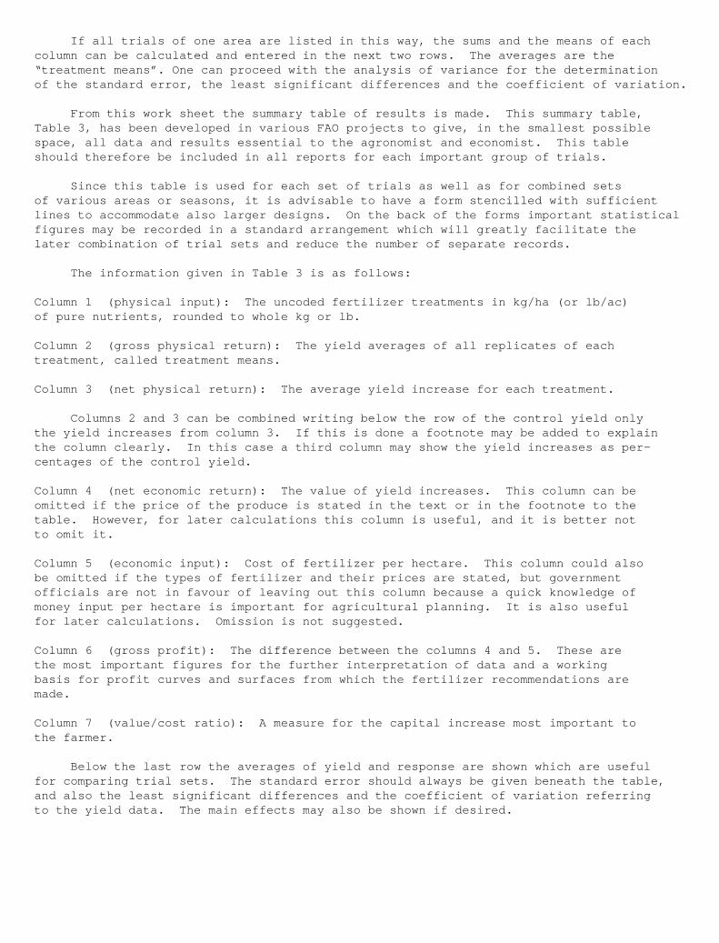
If all trials of one area are listed in this way, the sums and the means of eachcolumn can be calculated and entered in the next two rows. The averages are the“treatment means”. One can proceed with the analysis of variance for the determinationof the standard error, the least significant differences and the coefficient of variation.

From this work sheet the summary table of results is made. This summary table,Table 3, has been developed in various FAO projects to give, in the smallest possiblespace, all data and results essential to the agronomist and economist. This tableshould therefore be included in all reports for each important group of trials.

Since this table is used for each set of trials as well as for combined setsof various areas or seasons, it is advisable to have a form stencilled with sufficientlines to accommodate also larger designs. On the back of the forms important statisticalfigures may be recorded in a standard arrangement which will greatly facilitate thelater combination of trial sets and reduce the number of separate records.

The information given in Table 3 is as follows:

Column 1 (physical input): The uncoded fertilizer treatments in kg/ha (or lb/ac)of pure nutrients, rounded to whole kg or lb.

Column 2 (gross physical return): The yield averages of all replicates of eachtreatment, called treatment means.

Column 3 (net physical return): The average yield increase for each treatment.

Columns 2 and 3 can be combined writing below the row of the control yield onlythe yield increases from column 3. If this is done a footnote may be added to explainthe column clearly. In this case a third column may show the yield increases as per-centages of the control yield.

Column 4 (net economic return): The value of yield increases. This column can beomitted if the price of the produce is stated in the text or in the footnote to thetable. However, for later calculations this column is useful, and it is better notto omit it.

Column 5 (economic input): Cost of fertilizer per hectare. This column could alsobe omitted if the types of fertilizer and their prices are stated, but governmentofficials are not in favour of leaving out this column because a quick knowledge ofmoney input per hectare is important for agricultural planning. It is also usefulfor later calculations. Omission is not suggested.

Column 6 (gross profit): The difference between the columns 4 and 5. These arethe most important figures for the further interpretation of data and a workingbasis for profit curves and surfaces from which the fertilizer recommendations aremade.

Column 7 (value/cost ratio): A measure for the capital increase most important tothe farmer.

Below the last row the averages of yield and response are shown which are usefulfor comparing trial sets. The standard error should always be given beneath the table,and also the least significant differences and the coefficient of variation referringto the yield data. The main effects may also be shown if desired.

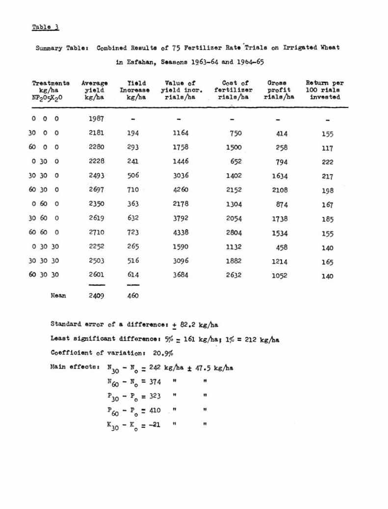
Table 3

Summary Tabla: Combined Resulte of 75 Fertilizer Rate'Trials on Irrigated Wheat

in Esfahan, Seasons 1963-64 and 1964-65

Standard error of a difference: + 82.2 kg/ha

Least significant difforence: = 161 kg/ha; leis," = 212 kg/ha

Coefficient of variation: 20.9;fo

Main effects:N30

N 242 kg/ha j47.5 kg/hao

N60 No = 374

P30 Po = 323

p60 -Po T 410K K 2130 0 -

Treatmentskg/ha

NP205K20

Averageyieldkg/ha

YieldInoreasekg/ha

Value ofyield incr.rials/ha

Cost offertilizerriada/ha

Grossprofitrials/ha

Return per100 Haleinvested

o o o 1987 - _

30 o o 2181 194 1164 750 414 155

60 o o 2280 293 1758 1500 258 117

030 0 2228 241 1446 652 794 222

30 30 0 2493 506 3036 1402 1634 217

60 30 0 2697 710 4260 2152 2108 198

060 0 2350 363 2178 1304 874 167

30 60 0 2619 632 3792 2054 1738 185

60 60 0 2710 723 4338 2804 1534 155

0 30 30 2252 265 1590 1132 458 140

30 30 30 2503 516 3096 1882 1214 165

60 30 30 2601 614 3684 2632 1052 140

Mean 2409 460

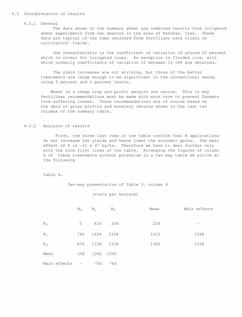
4.3 Interpretation of results

4.3.1 General The data shown in the summary sheet are combined results from irrigated wheat experiments from two seasons in the area of Esfahan, Iran. These data are typical of the type obtained from fertilizer rate trials on cultivators’ fields.

One characteristic is the coefficient of variation of around 20 percent which is normal for irrigated crops. An exception is flooded rice, with which normally coefficients of variation of between 12-18% are obtained.

The yield increases are not striking, but those of the better treatments are large enough to be significant in the conventional sense, using 5 percent and 1 percent levels.

Wheat is a cheap crop and profit margins are narrow. This is why fertilizer recommendations must be made with much care to prevent farmers from suffering losses. These recommendations are of course based on the data of gross profits and monetary returns shown in the last two columns of the summary table.

4·3.2 Analysis of results

First, the three last rows of the table confirm that K applications do not increase the yields and hence lower the economic gains. The main effect of K is -21 ± 47 kg/ha. Therefore we have to deal further only with the nine first lines of the table. Arranging the figures of column 6 of these treatments without potassium in a two-way table we arrive at the following

Table 4.

Two-way presentation of Table 3, column 6

(rials per hectare)

N o N 1 N 2 Mean Main effects

P 0 0 414 258 224 —

P 1 794 1634 2108 1512 1288

P 2 874 1738 1534 1382 1158

Mean 556 1262 1300

Main effects - 706 744

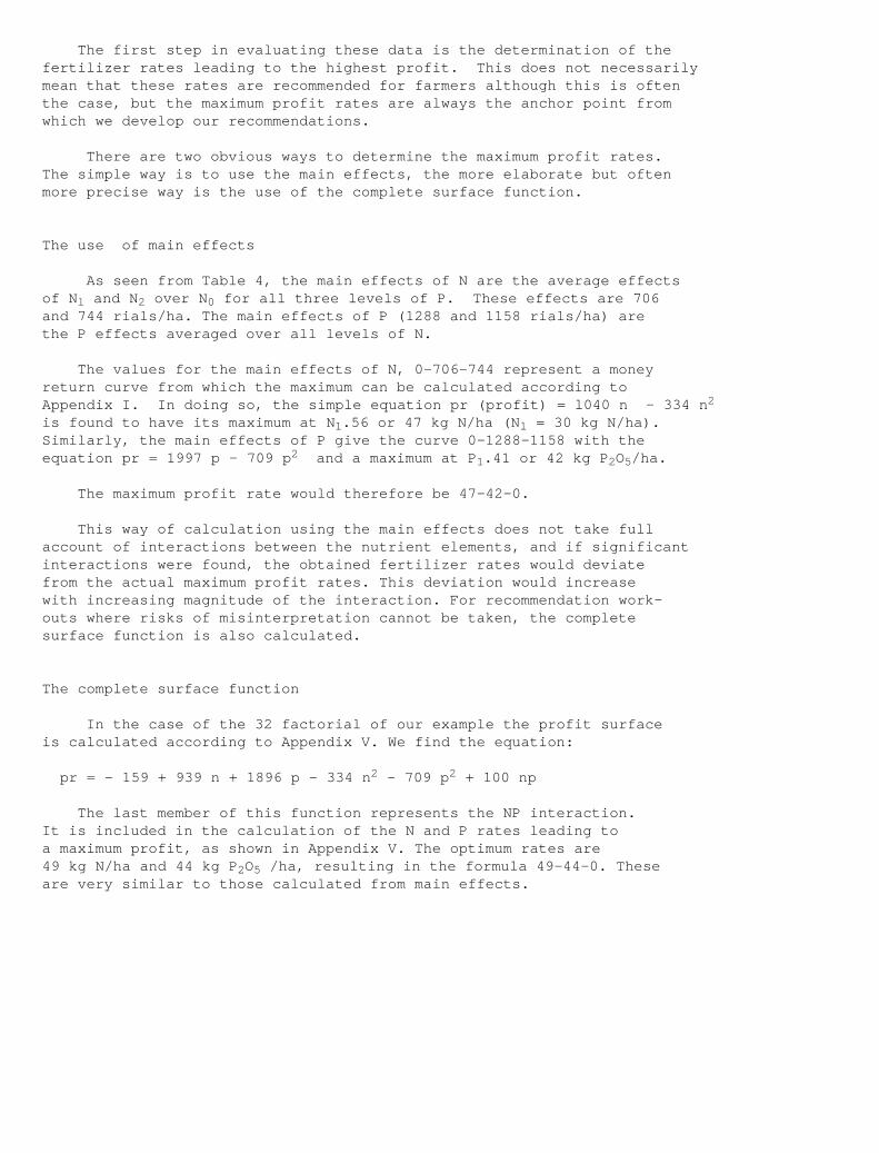
The first step in evaluating these data is the determination of thefertilizer rates leading to the highest profit. This does not necessarilymean that these rates are recommended for farmers although this is oftenthe case, but the maximum profit rates are always the anchor point fromwhich we develop our recommendations.

There are two obvious ways to determine the maximum profit rates.The simple way is to use the main effects, the more elaborate but oftenmore precise way is the use of the complete surface function.

The use of main effects

As seen from Table 4, the main effects of N are the average effectsof N l and N 2 over N 0 for all three levels of P. These effects are 706and 744 rials/ha. The main effects of P (1288 and 1158 rials/ha) arethe P effects averaged over all levels of N.

The values for the main effects of N, 0-706-744 represent a moneyreturn curve from which the maximum can be calculated according toAppendix I. In doing so, the simple equation pr (profit) = l040 n - 334 n 2

is found to have its maximum at N 1.56 or 47 kg N/ha (N l = 30 kg N/ha).Similarly, the main effects of P give the curve 0-1288-1158 with theequation pr = 1997 p - 709 p 2 and a maximum at P 1.41 or 42 kg P 2O5/ha.

The maximum profit rate would therefore be 47-42-0.

This way of calculation using the main effects does not take fullaccount of interactions between the nutrient elements, and if significantinteractions were found, the obtained fertilizer rates would deviatefrom the actual maximum profit rates. This deviation would increasewith increasing magnitude of the interaction. For recommendation work-outs where risks of misinterpretation cannot be taken, the completesurface function is also calculated.

The complete surface function

In the case of the 32 factorial of our example the profit surfaceis calculated according to Appendix V. We find the equation:

pr = - 159 + 939 n + 1896 p - 334 n 2 - 709 p 2 + 100 np

The last member of this function represents the NP interaction.It is included in the calculation of the N and P rates leading toa maximum profit, as shown in Appendix V. The optimum rates are49 kg N/ha and 44 kg P 2O5 /ha, resulting in the formula 49-44-0. Theseare very similar to those calculated from main effects.

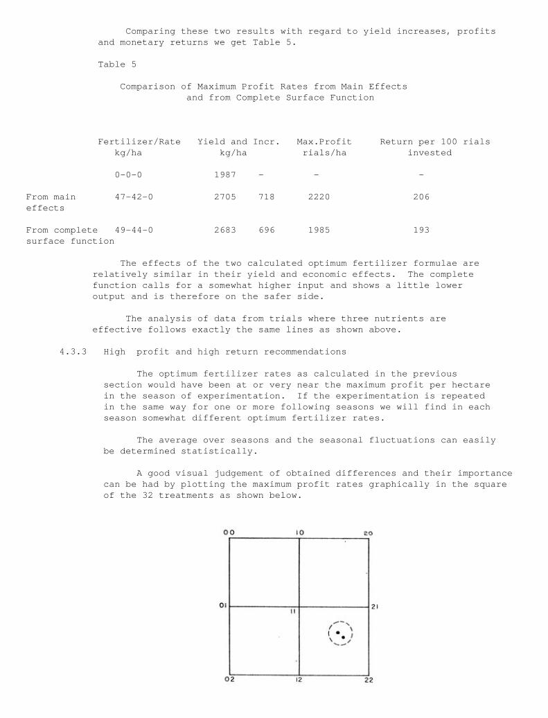
II

----,/ \I. i

,-...-/

02 12 22

0 0 i 0

Comparing these two results with regard to yield increases, profits and monetary returns we get Table 5.

Table 5

Comparison of Maximum Profit Rates from Main Effects and from Complete Surface Function

Fertilizer/Rate Yield and Incr. Max.Profit Return per 100 rials kg/ha kg/ha rials/ha invested

0-0-0 1987 - - -

From main 47-42-0 2705 718 2220 206effects

From complete 49-44-0 2683 696 1985 193surface function

The effects of the two calculated optimum fertilizer formulae are relatively similar in their yield and economic effects. The complete function calls for a somewhat higher input and shows a little lower output and is therefore on the safer side.

The analysis of data from trials where three nutrients are effective follows exactly the same lines as shown above.

4.3.3 High profit and high return recommendations

The optimum fertilizer rates as calculated in the previous section would have been at or very near the maximum profit per hectare in the season of experimentation. If the experimentation is repeated in the same way for one or more following seasons we will find in each season somewhat different optimum fertilizer rates.

The average over seasons and the seasonal fluctuations can easily be determined statistically.

A good visual judgement of obtained differences and their importance can be had by plotting the maximum profit rates graphically in the square of the 32 treatments as shown below.

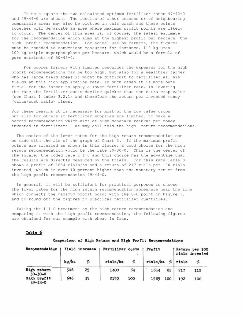
Table 6

Comparison of High Return and High Profit Recommendations

49-44-0

Reoommendation Tield increase Fertilizer oosts Pro fit Return per 100rials invented

kg/ha rials/ba 5 riale/ha % rialsHigb return 506 25 1400 64 1634 82 217 112

30-30-0High profit 696 35 2190 100 1985 100 192 100

In this square the two calculated optimum fertilizer rates 47-42-0and 49-44-0 are shown. The results of other seasons or of neighbouringcomparable areas may also be plotted in this graph and these pointstogether will demarcate an area where maximum profit points are likelyto occur. The center of this area is, of course, the safest estimatefor the recommendation which aims at the highest profit per hectare, thehigh profit recommendation. For actual use by farmers, the figuresmust be rounded to convenient measures; for instance, 110 kg urea +100 kg triple superphosphate per hectare, which would be a formula ofpure nutrients of 50-46-0.

For poorer farmers with limited resources the expenses for the highprofit recommendations may be too high. But also for a wealthier farmerwho has large field areas it might be difficult to fertilizer all hisfields at this high application rate. In such cases it is more bene-ficial for the farmer to apply a lower fertilizer rate. In loweringthe rate the fertilizer costs decline quicker than the extra crop value(see Chart 1 under 3.2.1) and therefore the return per invested money(value/cost ratio) rises.

For these reasons it is necessary for most of the low value cropsbut also for others if fertilizer supplies are limited, to make asecond recommendation which aims at high monetary returns per moneyinvested in fertilizers. We may call this the high return recommendations.

The choice of the lower rates for the high return recommendation canbe made with the aid of the graph of Chart 3. If the maximum profitpoints are situated as shown in this figure, a good choice for the highreturn recommendation would be the rate 30-30-0. This is the center ofthe square, the coded rate 1-1-0 and this choice has the advantage thatthe results are directly measured by the trials. For this rate Table 3shows a profit of 1634 rials/ha and a return of 217 rials per 100 rialsinvested, which is over 10 percent higher than the monetary return fromthe high profit recommendation 49-44-0.

In general, it will be sufficient for practical purposes to choosethe lower rates for the high return recommendation somewhere near the linewhich connects the maximum profit point with the 0-0 point in Figure 3,and to round off the figures to practical fertilizer quantities.

Taking the 1-1-0 treatment as the high return recommendation andcomparing it with the high profit recommendation, the following figuresare obtained for our example with wheat in Iran.

Taking the fertilizer costs and profit per hectare for the highprofit recommendation as l00 percent the high return recommendation is36 percent cheaper, but the profit is only 18 percent lower and con-sequemtly the return per invested capital is higher, in this case 12percent. The yield increase due to the high return recommendation is10 percent lower than that with the high profit recommendation.

The safety of these fertilizer recommandations is actually expressedin the value/cost ratio of about 2 (last column). It is obvious that invery good seasons the responses, profits, and returns will be higher andin bad seasons lower. However, with a value/cost ratio of 2 or higherthe chances for a farmer to suffer financial loss from fertilizer useare very small and, therefore, 2 is taken usually as the lower limitfor the value/cost ratio in developing countries.

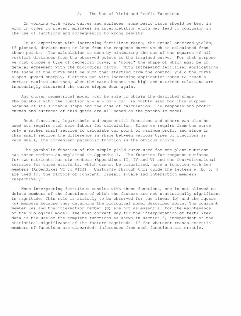
5. The Use of Yield and Profit Functions

In vorking with yield curves and surfaces, some basic facts should be kept inmind in order to prevent mistakes in interpretation which may lead to confusion inthe use of functions and consequently to wrong results.

In an experiment with increasing fertilizer rates, the actual observed yields,if plotted, deviate more or less from the response curve which is calculated fromthese points. The calculation is done by minimizing the sum of the squares of allvertical distances from the observed points to the imagined curve. For that purposewe must choose a type of geometric curve, a “model” the shape of which must be ingeneral agreement with the biological facts. With increaaing fertilizer applicationsthe shape of the curve must be such that starting from the control yield the curveslopes upward steeply, flattens out with increasing application rates to reach acertain maximum and then, when the rates become too high and nutrient relations areincreasingly disturbed the curve slopes down again.

Any chosen geometrical model must be able to obtain the described shape.The parabola with the function y = a + bx + cx 2 is mostly used for this purposebecause of its suitable shape and the case of calculation. The response and profitcurves and surfaces of this guide are all based on the parabolic model.

Root functions, logarithmic and exponential functions and others can also beused but require much more labour for calculation. Since we require from the curveonly a rather small section to calculate our point of maximum profit and since inthis small section the difference in shape between various types of functions isvery small, the convenient parabolic function is the obvious choice.

The parabolic function of the simple yield curve used for one plant nutrienthas three members as explained in Appendix I. The function for response surfacesfor two nutrients has six members (Appendixes II, IV and V) and the four-dimensionalsurfaces for three nutrients, which cannot be visualized, have a function with tenmembers (Appendixes VI to VIII). Uniformly through this guide the letters a, b, c, dare used for the factors of constant, linear, square and interaction membersrespectively.

When interpreting fertilizer results with these functions, one is not allowed todelete members of the functions of which the factors are not statistically significantin magnitude. This rule is strictly to be observed for the linear (b) and the square(c) members because they determine the biological model described above. The constantmember (a) and the interaction member (d) are not as essential for the maintenanceof the biological model. The most correct way for the interpretation of fertilizerdata is the use of the complete functions as shown in section 3, independent of thestatistical significance of the factors magnitude. If for whatever reason essentialmembers of functions are discarded, inferences from such functions are erratic.

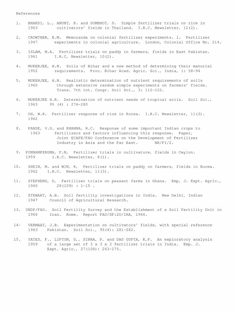
References

l. BHAKDI, L., ANUNT, K. and SOMBHOT, S. Simple fertilizer trials on rice in 1963 cultivators’ fields in Thailand. I.R.C. Newsletter, 12(2).

2. CROWTHER, E.M. Memoranda on colonial fertilizer experiments. l. Fertilizer 1947 experiments in colonial agriculture. London, Colonial Office No. 214.

3. ISLAM, M.A. Fertilizer trials on paddy in farmers, fields in East Pakistan. 1961 I.R.C, Newsletter, 10(2).

4. MUKERJEE, H.N. Soils of Bihar and a new method of determining their manurial 1952 requirements. Proc. Bihar Acad. Agric. Sci., India, l: 58-94

5. MUKERJEE, H.N. Realistic determination of nutrient requirements of soils 1960 through extensive random simple experiments on farmers’ fields. Trans. 7th int. Congr. Soil Sci., 3: 112-122.

6. MUKERJEE H.R. Determination of nutrient needs of tropical soils. Soil Sci., 1963 95 (4) : 276-280

7. OH, W.K. Fertilizer response of rice in Korea. I.R.C. Newsletter, 11(3). 1962

8. PANSE, V.G. and KHANNA, R.C. Response of some important Indian crops to 1963 fertilizers and factors influencing this response. Paper, Joint ECAFE/FAO Conference on the Development of Fertilizer Industry in Asia and the Far East. NR/FI/2.

9. PONNAMPERUMA, F.N, Fertilizer trials in oultivatore, fields in Ceylon. 1959 I.R.C. Newsletter, 8(1).

10. SHEIN, M. and WIN, K, Fertilizer trials on paddy on farmers, fields in Burma. 1962 I.R.C. Newsletter, 11(3).

11. STEPHENS, D, Fertilizer trials on peasant farms in Ghana. Emp, J. Expt. Agric., 1960 28(l09) : 1-15 .

12. STEWART, A.B. Soil fertility investigations in India. New Delhi, Indian 1947 Council of Agricultural Research.

13. UNDP/FAO. Soil Fertility Survey and the Establishment of a Soil Fertility Unit in 1966 Iran. Rome. Report FAO/SF:2O/IRA, 1966.

14· VERMAAT, J.B. Experimentation on cultivators’ fields, with special reference 1963 Pakistan. Soil Sci., 95(4): 281-282.

15. YATES, F., LIPTON, S,, SINHA, P, and DAS GUPTA, K,P. An exploratory analysis 1959 of a large set of 3 x 3 x 3 fertilizer trials in India. Emp. J. Expt. Agric., 27(108): 263-275.

Yields

General function y a + bx + cx2

y = yield i fertilizer rates

factor a = control yield C at x = 0

b = slope of the curve at x = 0

o = measure of "downpull" of curveif o is negative.

With positive o curve bends. upward.

APPENDIX I

Calculation of a Parabolic Return Curve from FertilizerRates 0, 1, 2 and Relation Between Yield and Profit Fanction

From the meaaured yields C, A, B the factors a, b, o are calculatedas follows:

a = C

b = 4A - B - 3C2 (1)

o z B + C - 2A2

If o is negative the curve bends downward (this should be the case) and thefertilizer rate x at whioh the yield is maximum is

- bmax

2o

To calculate y the value for x is inserted in the original function.max max

A quioker way of oalculatin g ymax is the equation

Y a + 1 bxmaxmax 2

(2)

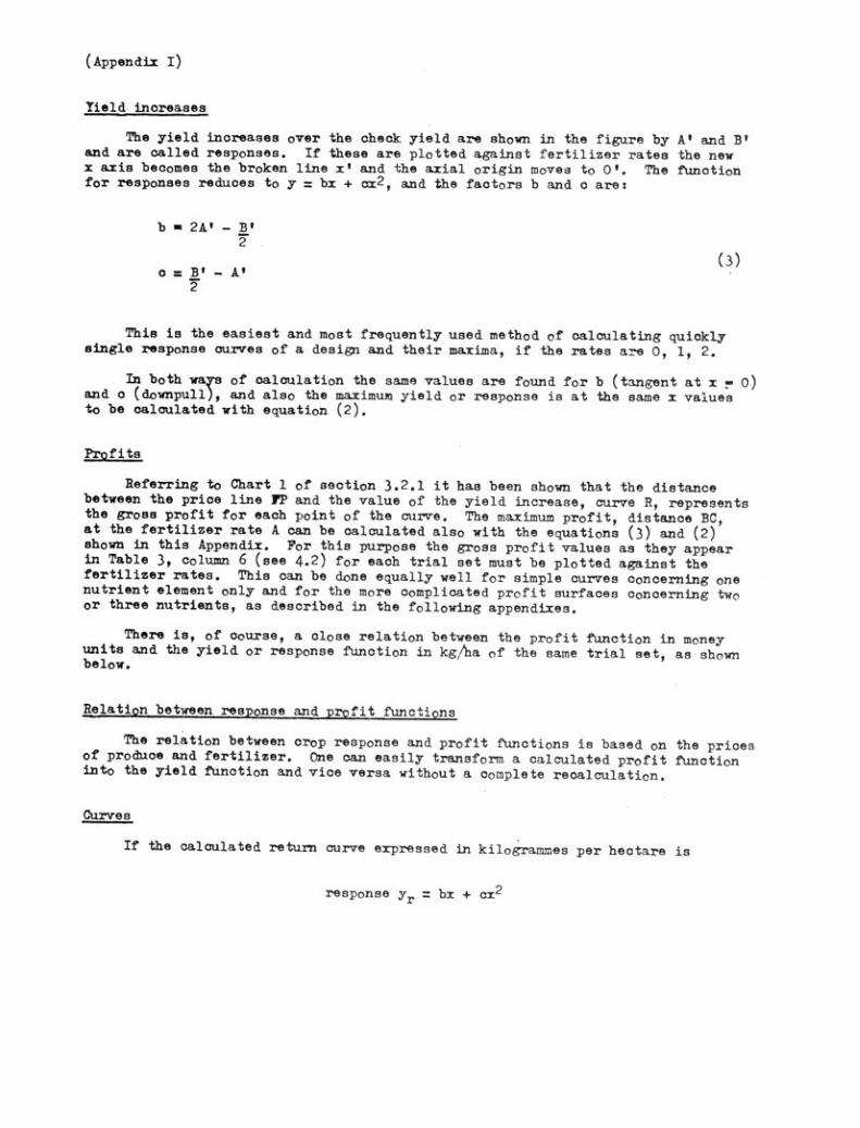
(Appendix I)

Yield increases

The yield increases over the check yield are shown in the figure by A' and B'and are called responses. If these are plotted against fertilizer ratea the newx axis becomes the broken line x' and the axial origin moves to 0'. The functionfor responses reduces to y = bx + ax2, and the faotors b and o are:

b 2A' - B1

o = B' - A'

This in the easiest and most frequently used method of calculating quioklysingle response curves of a design and their maxima, if the rates are 0, 1, 2.

In both wayn of calculation the same values are found for b (tangent at x r 0)and o (downpull), and also the maximum yield or response is at the same x valuesto be calculated with equation (2).

Profits

Referring to Chart 1 of section 3.2.1 it has been shown that the distancebetween the price line FP and the value of the yield increase, curve R, representsthe grosa profit for each point of the curve. The maximum profit, distance BC,at the fertilizer rate A can be calculated also with the equations (3) and (2)shown in this Appendix. For this purpose the gross profit values as they appearin Table 3, column 6 (see 4.2) for each trial set must be plotted against thefertilizer rates. This can be done equally well for simple curves concerning onenutrient element only and for the more complicated profit surfaces concerning twoor three nutrients, as described in the following appendixes.

There is, of course, a close relation between the profit function in moneyunits and the yield or response function in kg/ha of the name trial set, as shownbelow.

Relation between response and profit functions

The relation between crop response and profit functions is based on the pricesof produce and fertilizer. One can easily transform a calaulated profit functioninto the yield function and vice versa without a complete reoalculaticn.

Curves

If the calculated return curve expressed in kilogrammes per heotare is

response yr = bx + cx2

( 3)

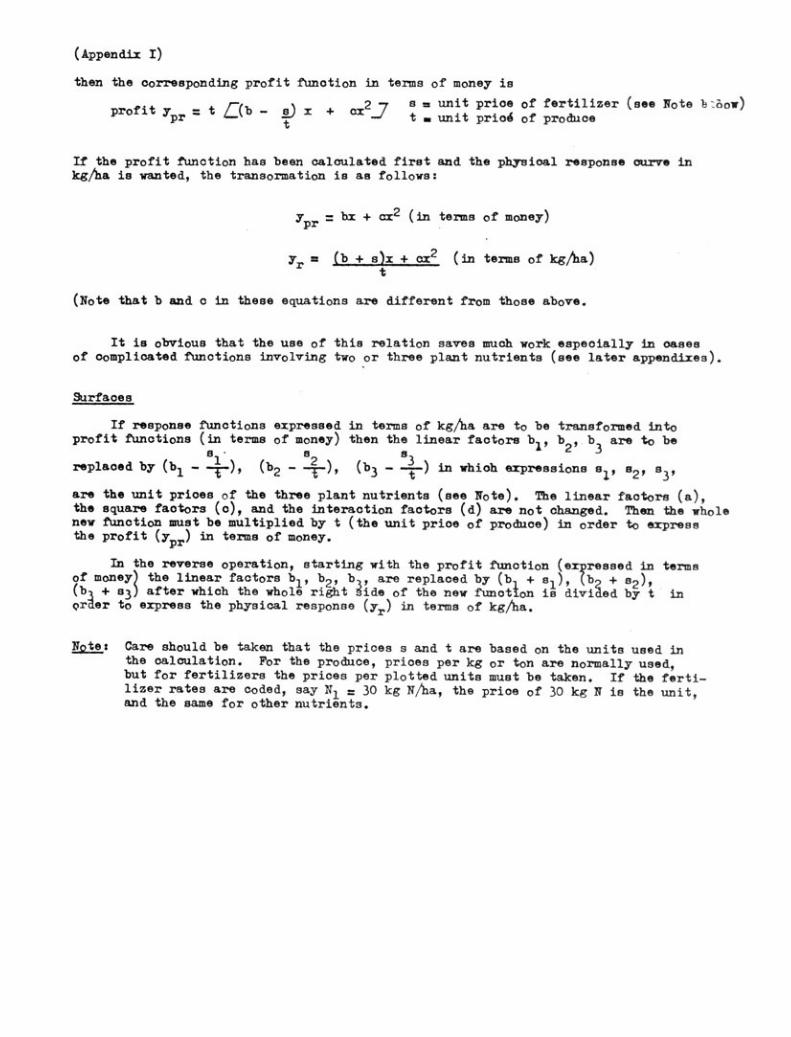
(Appendix I)

then the corresponding profit funotion in terms of money is

profit y - +s . unit prioe of fertilizer (see Note blflow)= t f."(b 2) x ax22pr t . unit prio4 of produce

If the profit function has been calculated first and the physical response curve inkg/ha is wanted, the transormation is as follows:

/y = bx + 2.ax in terms øf money)pr

yr = (b + 8)x + cx2 (in terms of kg/ha)

(Note that b and c in these equations are different from those above.

It is obvious that the use of this relation saves much work espeoially in oasesof complicated functions involving two or three plant nutrients (see later appendixes).

Surfaces

If response functions expressed in terms of kg/ha are to be transformed intoprofit functions (in terms of money) then the linear faotore b1, b2' b3 are to be

81 83replaced by (b1 - -7), (b2 - 82 (b3 - -7) in whioh expressions 81,

are the unit prioes of the three plant nutrients (see Note). The linear faotors (a),the square factors (o), and the interaction faotors (d) are not changed. Then the wholenew function must be multiplied by t (the unit prioe of produce) in order to expressthe profit (y ) in terms of money.pr

In the reverse operation, starting with the profit function (expressed in termsof monel the linear factors bl, b2, 1)1, are replaced by (hi + el), (b2 + 82),(bA + 83 after which the whole right 6ide of the new function is divided by t tnoraer to express the physical response (yr) in terms of kg/ha.

Note: Care should be taken that the prices s and t are based on the units used inthe oalaulation. For the produce, prioes per kg or ton are normally used,but for fertilizers the prices per plotted units muot be taken. If the ferti-lizer rates are coded, say N1 30 kg N/ha, the price of 30 kg N in the unit,and the sane for other nutrients.

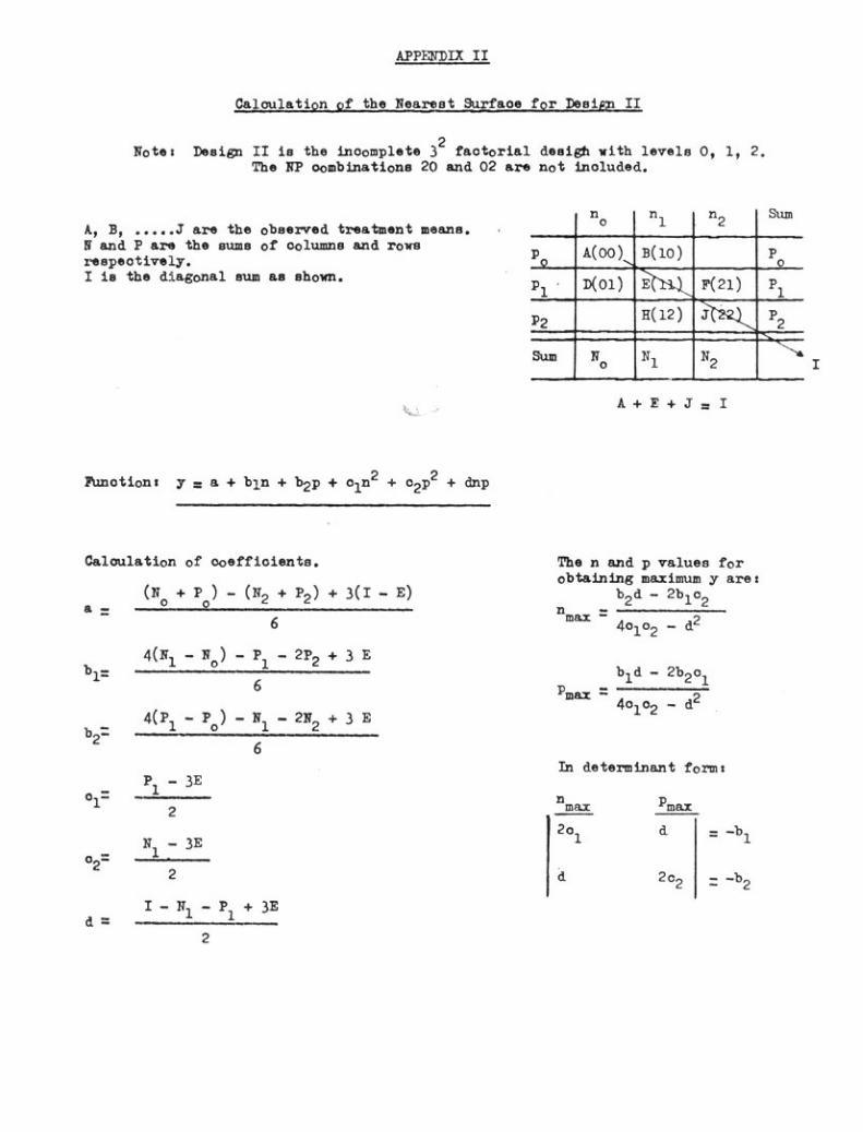
b1

b2=

o1=

o2=

dm

) P 2P4(N1 - No - 1 - 2 + 3 E

2

6

4(P1 - Po) - N1 - 2N2 + 3 E

6

P1 - 3E

2

N1 - 3E

2

I - N1 - P1 + 3E

APPIZTDIX II

Calculation of the Nearest Surface for Deeipp

Note: Design II is the inoomplete 32 factorial clef:JO, with levels 0, 1, 2.The AP oombinations 20 and 02 are not inoluded.

A, B, J are the observed treatment means.and P are the puma of columns and rows

respeotively.I is the diagonal sum as shown.

Funotionl y = a + bin + b2p + 01n2 + 02p2 + dnp

A+E+J=I

aaloulation of aoefficients. The n and p values forobtaining maximum y are:

(N + P ) - (N2 + P2) + 3(1 - E)b2d - 2b1o2a = o

6MAX -

40102 - d2

In determinant form:

max

2o1

PMELX

2c2

= -

no n1 n2Sstun

Po

A(00)-, B(10) P0

P D(01) , F(21) P11

P2H(12)

2

SumNo N1 N2

b1d - 2b2omax -

40102 - d2

(Appendix II)

If in the above Panotion the valuea of n and p are introduced,max max

obtained. A much quicker way of oalculating yami is the use of the

1y - a +(D1w' n_mx + b2pma1)max 2

which gives the same reffult. This equation ie only valid for parabolic functione andoannot be used for other than the maximum y value.

the ymax is

equation

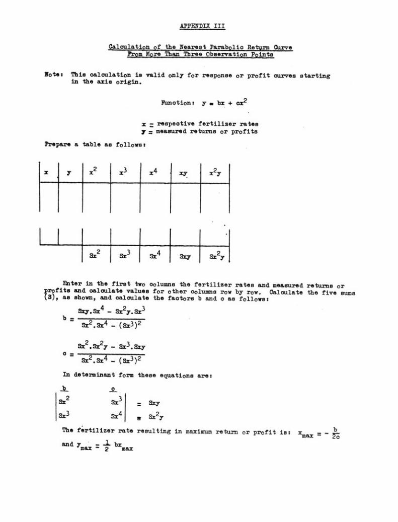
2ax

Calculation 2! the Nearest Parabolic Return Curve?ro m More Than Three Observation Pointe

Note: This oalculation is valid only for response or profit curves startingin the axis origin.

Funotion: y . bx + ax2

x respective fertilizer ratesy = measured returns or profits

Prepare a table an follows:

Enter in the first two columna the fertilizer rates and measured returns orprofits and oalaulate values for other oolumns row by row. Caloulate the five sums(3), as shown, and calculate the factors b and o an follows:

Sxy.Sx4 - Sr2y.Sx3s-x2.sx4 (sx3)2

Sx2.Sx2y - Sx3.Sxyo

3- x2.sx4 (sx3)2

In determinant form these equations are:

o

X3

sx3 sx4

APPENDIX III

Sxy

2x y

The fertilizer rate resulting in maximum return or profit io:xmax -

and y _-Lbxmax - 2 max

Sr2

ax3

sx3

sx4-..: ay

sx2y

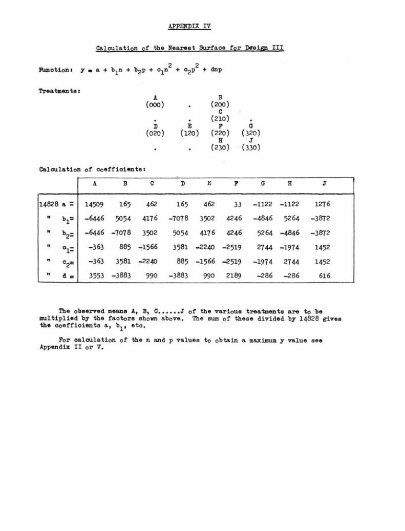
Calculation of ooeffioients:

APPENDIX IV

Calculation of the Nearest 3urface for Design III

Function: yma+b1n+ b2p +o1n2 + o2p2 + dnp

Treatments:A

The observed means A, B, C J of the various treatments are to bemultiplied by the factors shown above. The trUM of these divided by 14828 givesthe ooeffioients a, bl, etc.

For calculation of the n and p values to obtain a maximum y value seeAppendix II or 7.

A B C D E P 0 H .7

14828 a - 14509 165 462 165 462 33 -1122 -1122 1276

" 1)1= -6446 5054 4176 -7078 3502 4246 -4846 5264 -3872

" b2- - -6446 -7078 3502 5054 4176 4246 5264 -4846 -3872

" o1 - -363 885 -1566 3581 -2240 -2519 2744 -1974 1452

2- -363 3581 -2240 885 -1566 -2519 -1974 2744 1452

" d = 3553 -3883 990 -3883 990 2189 -286 -286 616

(000) (200)

(210)E F 0

(020) (120) (220) (320)

(230) (330)

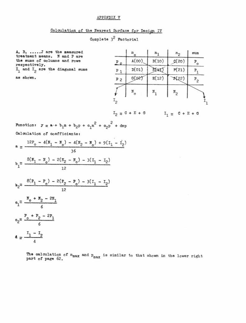
A, B, J are the measuredtreatment means. N and P arethe ¡name of oolumns and rowsrespectively.

and 12 ere the diagonal mums

Le shawn.

a

36

APPEgDIX 7

Calculation of the Nearest Surface for DesiloniV

Complete 32 Factorial

a(p -P ) - 2(P2 - Po) - 3(11 -2)1b2 0-

12

- Po + P2 - 2P102

6

I1 - I2a4

The aalcu/ation of nm and p is similar to that shown in the lower rightax maxpart of page 62.

12 C4- E +2 -

2%notion: y = a.+ bin + b2p + oln2 + 02p + dnp

Calculation of aoeffioients:

12P0 - 4(N1 - Fo) - 4(N2 - Fo) + - 12)

I - C + E + 01 -

no n1 n2 sum

2._CA(00) B(10) C(20) Po

P1 D(01) F(21)P1

P 2 2Y H(12 522)P2

No

N1

N2

b8(51 - 50) 2(N2 50) 3(11 12)

112

- No + N2 - 2V1ol

6

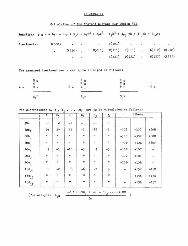
A-

B

=

B =C

D

sl

(for example: 1)1=

s2--

APPFSDIX VI

Calculation of the Nearest Surface for Denim VII

Funotiont y = a + bin + b2p + b3k + o1n2 + c2p2 + o3k2 + d23 pk,+ d13nk + d12np

Treatments: A(000) . C(101) . .

m(110) . B(011) H(111) J(211) . L(112) N(212)

K(121) p(221) . s(122) Q(222)

The measured treatment means are to be arranged as follows:

M

N 7.

P

S3=

-29A + 29S1 + 34B - 352

60

+60M

I

A S1 HS2 S3 4 rthers

i

30a 26 4 -1 -3 -1 5

60h1-29 29 34 -3 -26 -5 -90B +303 +60M

60b2"

11 II II 11 -90C +30K +6017

60b II It 11 II n u -90D +30L +60P3

20e11 -1 -16 -3 4 -5 +10B +103 -

200211 II " " " It +10C +10K _

20o It Il 11 11 11 Il +10D +10L _3

15d23 2 -2 8 -6 -7 5 - +153 +15M

1541..13

'I 9 Il II It 11 - +15K +1517

15d12

II II 11 II II II. - +15L +15P

The coefficients a, bi, b2 . . . .d12 are to be calculated as follows:

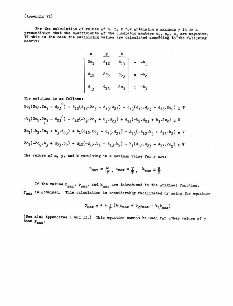
(Appendix VI)

For the calculation of values of n, p, k for obtaining a maximum y it is aprecondition that the coefficients of the quadratic members cl, 02, 03 are negative.If this is the case the maximizing values are aalculated aocording to the following

The solutian is as follows:

,

201(202.203 - d32) - d12(d12.203 - dird23) + d13(d12.d23 - d13.2o2) = T

-y2o2.2o3 - d232) - d12(-b2.203 + b3.d23) + di3(-b2.d23 + b3.202) =

2o1(-b2.2o3 + b3.d23) + b (d1,-122°3 - d13.d23) 4113(-d121)3 + d13.b2) IT V

2o1(-202.b3 + d23.b2) - d12(-d b-12/-3 -

d-13/132) - b1(d12"123 d13'2°2) t I

The values of n, p, and k resulting in a maximum value for y are:

n - u p =V k -Wmax - -- max --T / T max -

If the values n , p , and k are introduced in the original function,108.2 MILX IIIRX

ymax is obtained. This aalculation is considerably facilitated by using the equation

ymax = a + i(b1nmax + b2pmax + b3kmax)

(See also Appendixes I and II.) This equation cannot be used for other values of ythan ymax.

matrix:

201

d12

13

=

-b1

-b2

-b3

d12

202

c123

d13

d23

203

APPUrDIX VII

Calculation of the Nearest Durface for Design VIII

Funotion: y . a + bin + b2p + b3k + c1n2 + c2p2 + c3k2 + d23pk + dunk + d12np

Treatments: A(000) 1101 . 1201D(110) B(011) H 1111 J(211

M 1Lpll 212

. 0(220) K 121 P(221 E(022) 22 Q 222

The measured treatment means are to be arranged as follows:

= E = = =A C = F H = K = = =

D G L P

13111118 Sl=S2=

03=4-

The coeffioients of the function are calculated as follows:

(for example: bl =

See also Appendix VI.

-3052A + 3662S - 610S2 +1

6048

+4320M

AS1 S2

HS3 s4

Q Others

,

,

18144a 15600 2576 -112 -1288 -1736 -392 2744 _ _ _ _

604811 -3052 3662 -610 1463 211 -1433 -1309 -9936B +864E +2160J +432074

6048b2., /I fl II II _9936c +864r +2160K +4320N

6048b3it Il IV u u u " -9936D +8640 +2160L +4320P

1814401 1708 -2846 1138 -2303 -3259 1553 469 +6480B +2592E +6480J -5184M

1814402u u H u u u " +6480C +2592F +6480K -5180

1814403u II Il u u u " +6480D +2592G +6480L -5184P

1134d23112 148 -260 7 -223 -19 133 -486B +486E +648J + 162M

1134c13,1

Il il II II II II II -486C +486F +648K + 162N

1134d12 II II , , u u u u -486D +4860 +648L + 162P

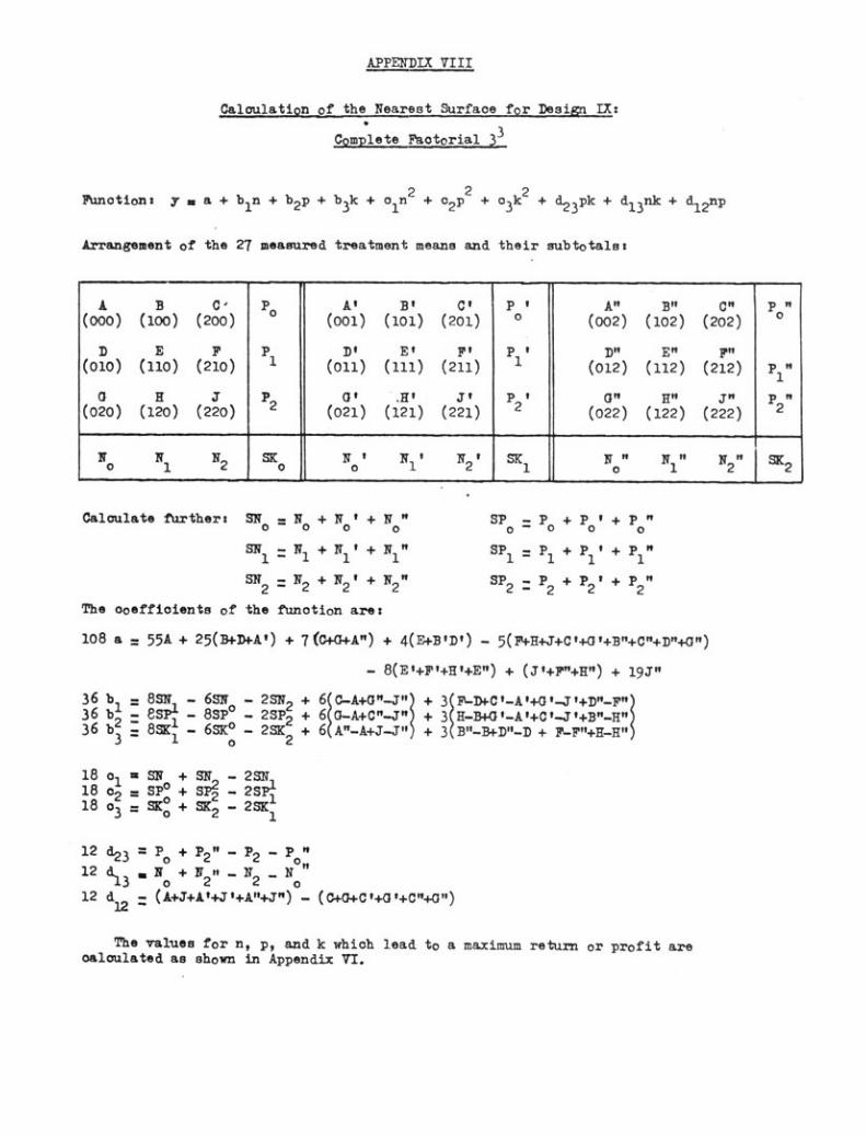
APPENDIX VIII

Calculation of the Neareot Surface for Design LK:

Complete Factorial 33

Funotion: y.a+b1n+ b2p + b3k +o1n2 + c2p2 + c3k2 + d-e_3pk +d13nk +d-

lenp

Arrangement of the 27 measured treatment meano and their nubtotals:

Calculate further: SN -N +N'+No"o - o o

SN -N +N'+111"1 - 1 1

3112 -N2 +N2I+ N2" SP2 -- P2 + P2 ' + P2"-The ooeffioients of the fmnotion are:

108 a = 55A + 25(B+D+A') + 7(CF0+A") + 4(E+BIDI) - 5(F+H+J+C,+01+B"+C"+D"+0")

- 8(El+P+HI+E") + (P+F"+H") + 19J"

36 b, = 8511 - 6311 - 23112 + 1C-A+G"-1 + 3r-104-C,-A0+0,-J1+D"-F"36 - es]" - 8sp° - 2sp2 + 6 G-A+C"-J" + 3 H-11.+0,-A,+CI-P+B"-H"36 b' 8SK' - 65K° - 23K + 6 A"-A+J-J" + 3 B"-B+D"-D + F-F"+H-H"

23 - 1 o

18 o, = SN + SN, - 2SN118 c2 = SP° + - 2SP'o18 03 = SK0 + SK2 -23K1

1

12 d23 = Po + P2" - P2 - Po"12 d13 . No + N2s - N2 _N12 d

-- (A+J+A'+.71+A"+J") - (C+0+C1+0P+C"+0")

12

The values for n, p, and k which lead to a maximum return or profit areoaloulated as shown in Appendix VI.

SP -P +PI+ P"o_ o o o

SP1 -P1 +P1'+ P1"-

A B C'P0

A' 131 C1 P' A" B" C" P"(000) (100) (200) (001) (101) (201) ° (002) (102) (202) e

D E F P D' E' F' P1' Dn E" Pm

(010) (110) (210) 1 (011) (111) (211) 1 (012) (112) (212) 151"

O H j P, O' .111 JI P,' 0" H J" P2"(020) (120) (220) ` (021) (121) (221) 4 (022) (122) (222) 2

No

N1 N2 SKo

N 'o

N '1 N2' SK

1N

o"

11i" N2" SK2