Observers and Kalman Filters

CS 393R: Autonomous Robots

Slides Courtesy of Benjamin Kuipers

Good Afternoon Colleagues

• Are there any questions?

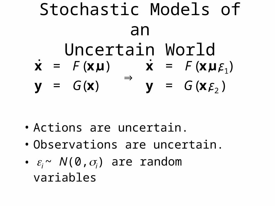
Stochastic Models of an

Uncertain World

• Actions are uncertain.• Observations are uncertain.

• i ~ N(0,i) are random variables

€

˙ x = F(x,u)

y = G(x)⇒

˙ x = F(x,u,ε1)

y = G(x,ε2)

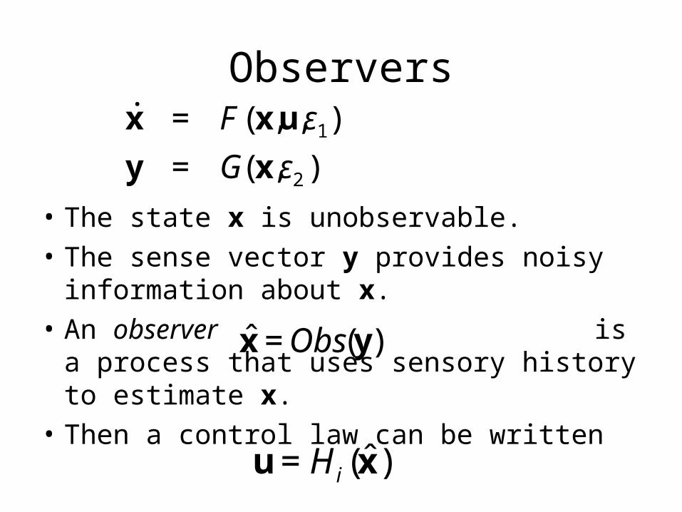
Observers

• The state x is unobservable.• The sense vector y provides noisy information about x.

• An observer is a process that uses sensory history to estimate x.

• Then a control law can be written

€

u=Hi(ˆ x )

€

˙ x = F(x,u,ε1)

y = G(x,ε2)

€

ˆ x =Obs(y)

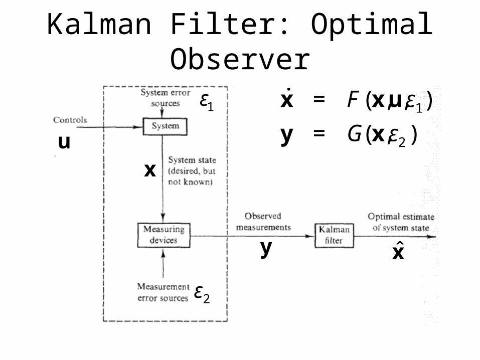
Kalman Filter: Optimal Observer

€

u

€

x

€

y

€

ˆ x

€

ε2

€

ε1

€

˙ x = F(x,u,ε1)

y = G(x,ε2)

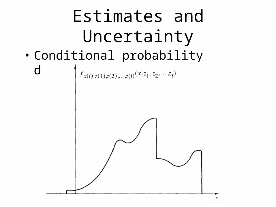
Estimates and Uncertainty

• Conditional probability density function

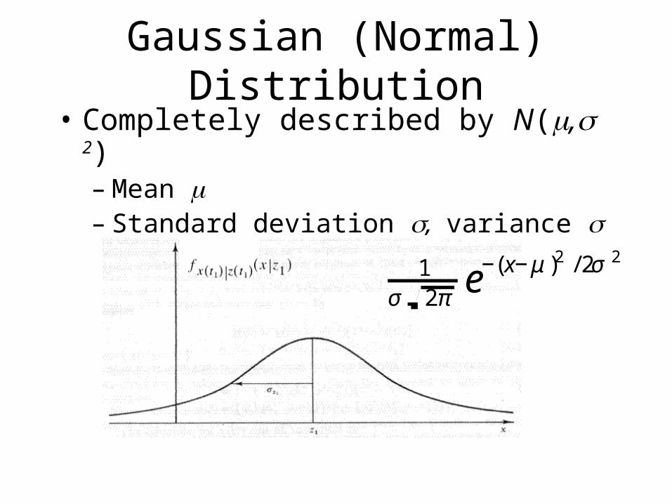
Gaussian (Normal) Distribution

• Completely described by N(, 2) – Mean – Standard deviation , variance 2

€

1σ 2π e−(x−μ)2 /2σ 2

The Central Limit Theorem

• The sum of many random variables– with the same mean, but– with arbitrary conditional density functions,

converges to a Gaussian density function.

• If a model omits many small unmodeled effects, then the resulting error should converge to a Gaussian density function.

Illustrating the Central Limit Thm

– Add 1, 2, 3, 4 variables from the same distribution.

Detecting Modeling Error

• Every model is incomplete.– If the omitted factors are all small, the resulting errors should add up to a Gaussian.

• If the error between a model and the data is not Gaussian, – Then some omitted factor is not small.

– One should find the dominant source of error and add it to the model.

Estimating a Value• Suppose there is a constant value x.– Distance to wall; angle to wall; etc.

• At time t1, observe value z1 with variance

• The optimal estimate is with variance

€

σ12

€

ˆ x (t1)=z1

€

σ12

A Second Observation

• At time t2, observe value z2 with variance

€

σ22

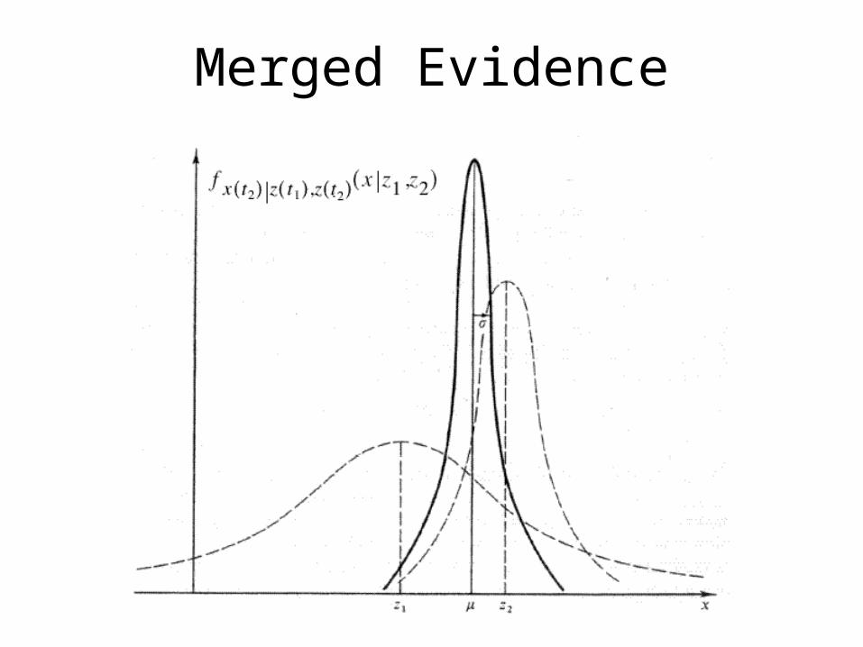
Merged Evidence

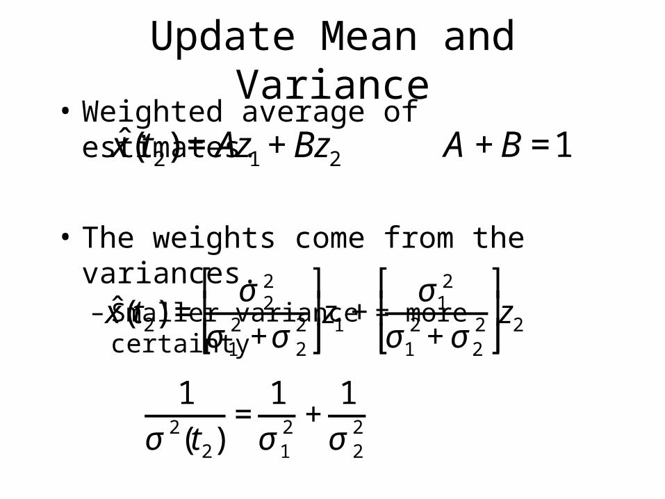
Update Mean and Variance

• Weighted average of estimates.

• The weights come from the variances.– Smaller variance = more certainty

€

ˆ x (t2) =Az1 +Bz2

€

ˆ x (t2) =σ 2

2

σ12 +σ 2

2

⎡

⎣ ⎢ ⎢

⎤

⎦ ⎥ ⎥ z1 +

σ12

σ12 +σ2

2

⎡

⎣ ⎢ ⎢

⎤

⎦ ⎥ ⎥ z2

€

1σ 2(t2)

=1

σ12 +

1σ 2

2

€

A+B=1

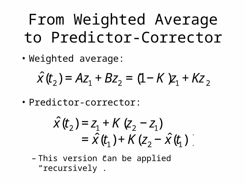
From Weighted Averageto Predictor-Corrector• Weighted average:

• Predictor-corrector:

– This version can be applied “recursively”.

€

ˆ x (t2) =Az1 +Bz2 =(1−K)z1 +Kz2

€

ˆ x (t2) =z1 +K(z2 −z1)

€

=ˆ x (t1)+K(z2 −ˆ x (t1))

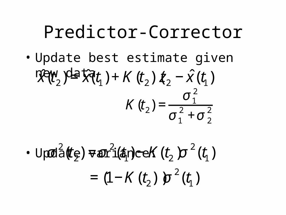
Predictor-Corrector• Update best estimate given new data

• Update variance:

€

ˆ x (t2) =ˆ x (t1)+K(t2)(z2 −ˆ x (t1))

€

K(t2) =σ1

2

σ12 +σ 2

2

€

σ 2(t2) =σ 2(t1)−K(t2)σ2(t1)

€

=(1−K(t2))σ2(t1)

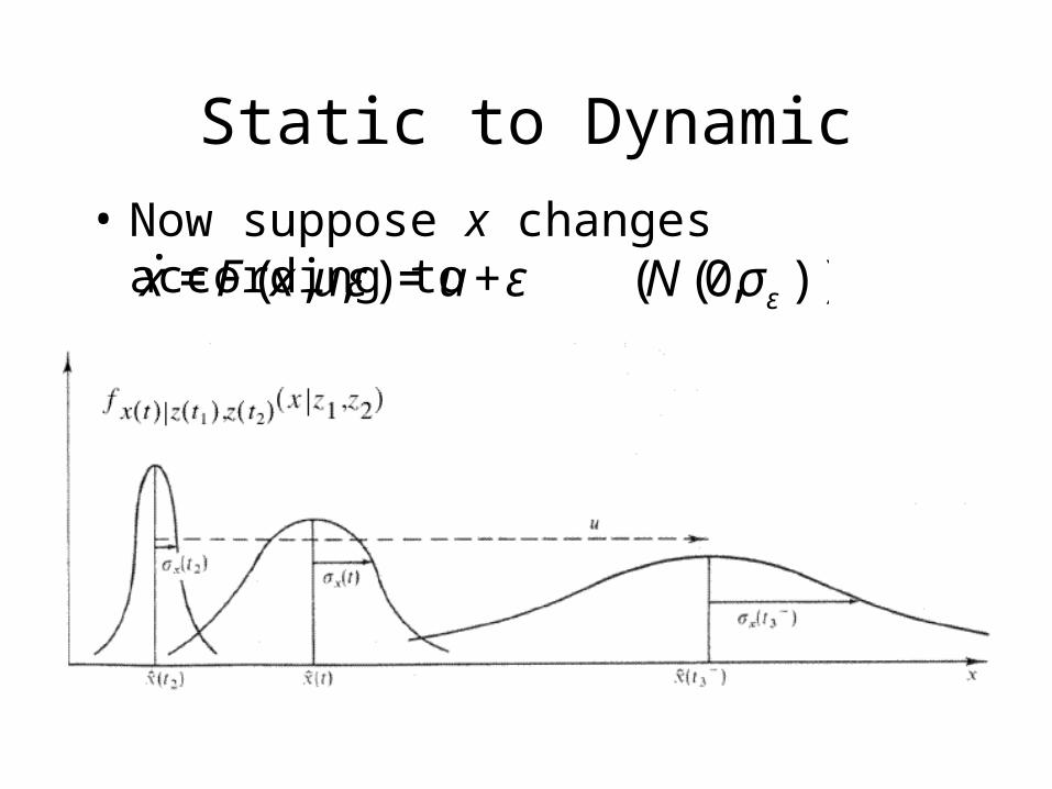
Static to Dynamic• Now suppose x changes according to

€

˙ x =F(x,u,ε)=u+ε (N(0,σε))

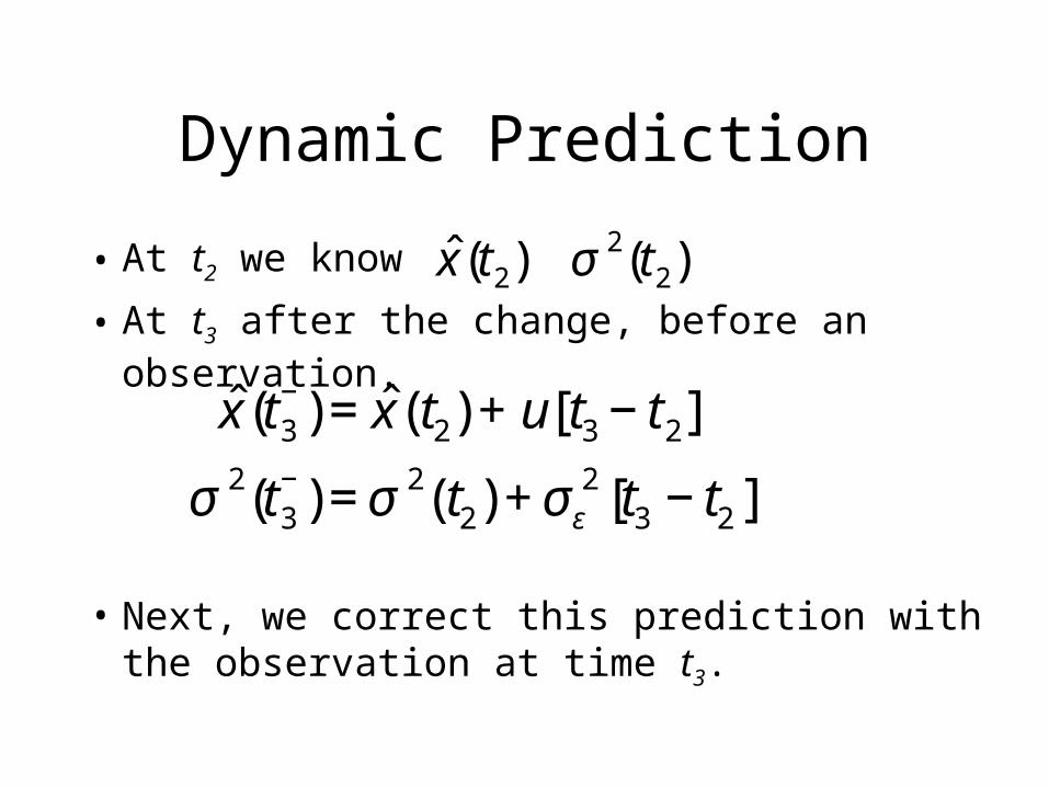
Dynamic Prediction

• At t2 we know

• At t3 after the change, before an observation.

• Next, we correct this prediction with the observation at time t3.

€

ˆ x (t3−)=ˆ x (t2)+u[t3 −t2]

€

σ 2(t3−)=σ 2(t2)+σε

2[t3 −t2]

€

ˆ x (t2) σ 2(t2)

Dynamic Correction

• At time t3 we observe z3 with variance

• Combine prediction with observation.

€

σ32

€

ˆ x (t3) =ˆ x (t3−)+K(t3)(z3 −ˆ x (t3

−))

€

K(t3) =σ 2(t3

−)σ 2(t3

−)+σ32

€

σ 2(t3) =(1−K(t3))σ2(t3

−)

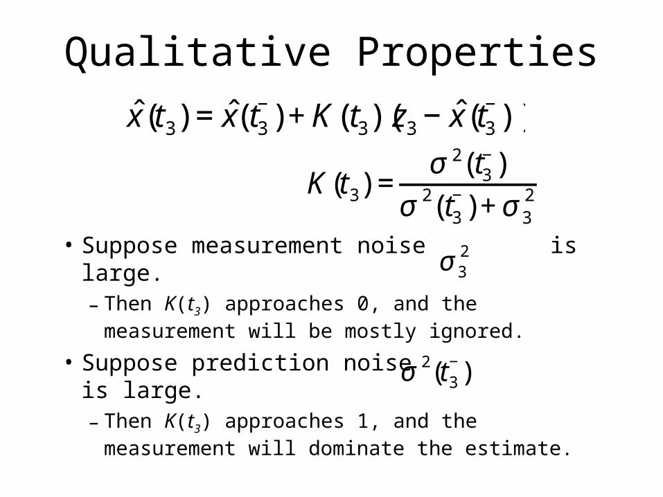
Qualitative Properties

• Suppose measurement noise is large.– Then K(t3) approaches 0, and the measurement will be mostly ignored.

• Suppose prediction noise is large.– Then K(t3) approaches 1, and the measurement will dominate the estimate.

€

K(t3) =σ 2(t3

−)σ 2(t3

−)+σ32

€

ˆ x (t3) =ˆ x (t3−)+K(t3)(z3 −ˆ x (t3

−))

€

σ32

€

σ 2(t3−)

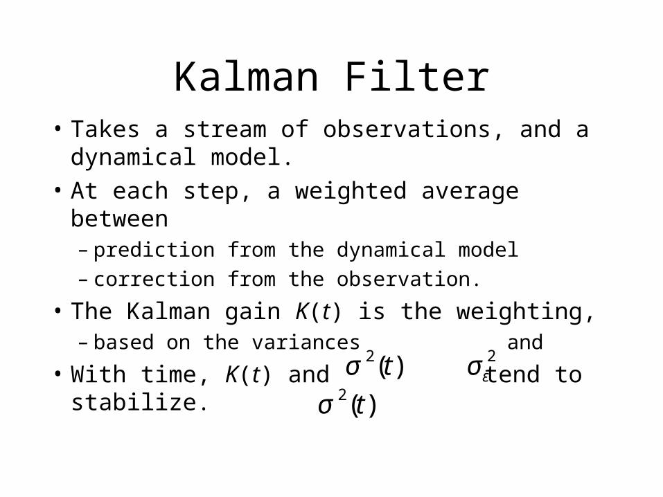
Kalman Filter• Takes a stream of observations, and a dynamical model.

• At each step, a weighted average between – prediction from the dynamical model– correction from the observation.

• The Kalman gain K(t) is the weighting,– based on the variances and

• With time, K(t) and tend to stabilize.

€

σ 2(t)

€

σε2

€

σ 2(t)

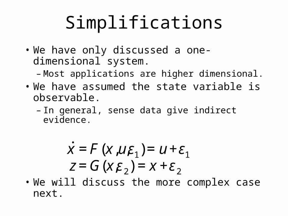
Simplifications• We have only discussed a one-dimensional system.– Most applications are higher dimensional.

• We have assumed the state variable is observable.– In general, sense data give indirect evidence.

• We will discuss the more complex case next.

€

˙ x =F(x,u,ε1)=u+ε1

€

z=G(x,ε2) =x+ε2

Up To Higher Dimensions

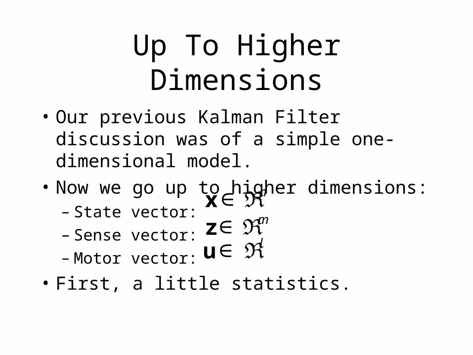
• Our previous Kalman Filter discussion was of a simple one-dimensional model.

• Now we go up to higher dimensions:– State vector: – Sense vector: – Motor vector:

• First, a little statistics.

€

x∈ℜn

€

z∈ℜm

€

u∈ℜl

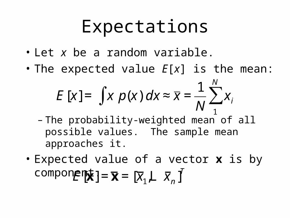
Expectations• Let x be a random variable. • The expected value E[x] is the mean:

– The probability-weighted mean of all possible values. The sample mean approaches it.

• Expected value of a vector x is by component.

€

E[x] = x p(x) dx∫ ≈ x =1

Nx i

1

N

∑

€

E[x]=x =[x 1,L x n]T

Variance and Covariance

• The variance is E[ (x-E[x])2 ]

• Covariance matrix is E[ (x-E[x])(x-E[x])T ]

– Divide by N1 to make the sample variance an unbiased estimator for the population variance.

€

σ 2 =E[(x−x )2]=1N

(xi −x )2

1

N

∑

€

Cij =1N

(xik −x i)(xjk −x j)k=1

N

∑

Covariance Matrix

• Along the diagonal, Cii are variances.

• Off-diagonal Cij are essentially correlations.

€

C1,1 = σ 12 C1,2 C1,N

C2,1 C2,2 = σ 22

O M

CN ,1 L CN ,N = σ N2

⎡

⎣

⎢ ⎢ ⎢ ⎢

⎤

⎦

⎥ ⎥ ⎥ ⎥

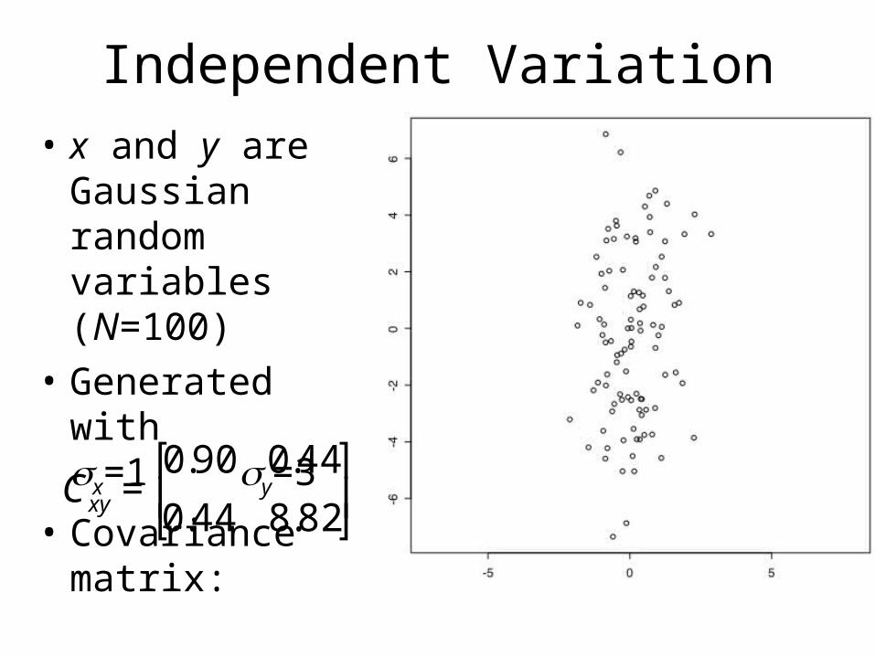
Independent Variation• x and y are Gaussian random variables (N=100)

• Generated with x=1 y=3

• Covariance matrix:

€

Cxy =0.90 0.44

0.44 8.82

⎡

⎣ ⎢

⎤

⎦ ⎥

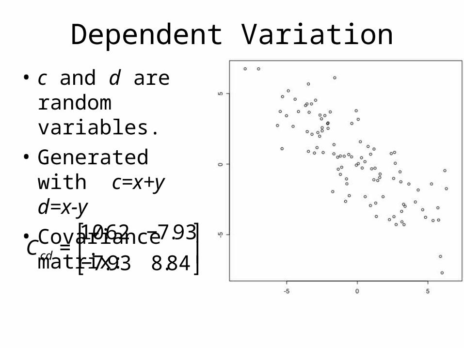
Dependent Variation• c and d are random variables.

• Generated with c=x+y d=x-y

• Covariance matrix:

€

Ccd =10.62 −7.93

−7.93 8.84

⎡

⎣ ⎢

⎤

⎦ ⎥

Discrete Kalman Filter• Estimate the state x n of a linear stochastic difference equation

– process noise w is drawn from N(0,Q), with covariance matrix Q.

• with a measurement z m

– measurement noise v is drawn from N(0,R), with covariance matrix R.

• A, Q are nn. B is nl. R is mm. H is mn.

€

x k = Ax k−1 + Buk−1 + wk−1

€

zk =Hxk +vk

Estimates and Errors• is the estimated state at time-step k.

• after prediction, before observation.

• Errors:

• Error covariance matrices:

• Kalman Filter’s task is to update

€

ˆ x k ∈ℜn

€

ˆ x k− ∈ℜn

€

ek−=xk −ˆ x k

−

ek =xk −ˆ x k

€

Pk−=E[ek

−ek−T

]

Pk =E[ek ekT ]

€

ˆ x k Pk

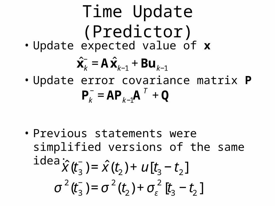
Time Update (Predictor)

• Update expected value of x

• Update error covariance matrix P

• Previous statements were simplified versions of the same idea:

€

ˆ x k− = Aˆ x k−1 + Buk−1

€

Pk−=APk−1A

T +Q

€

ˆ x (t3−)=ˆ x (t2)+u[t3 −t2]

€

σ 2(t3−)=σ 2(t2)+σε

2[t3 −t2]

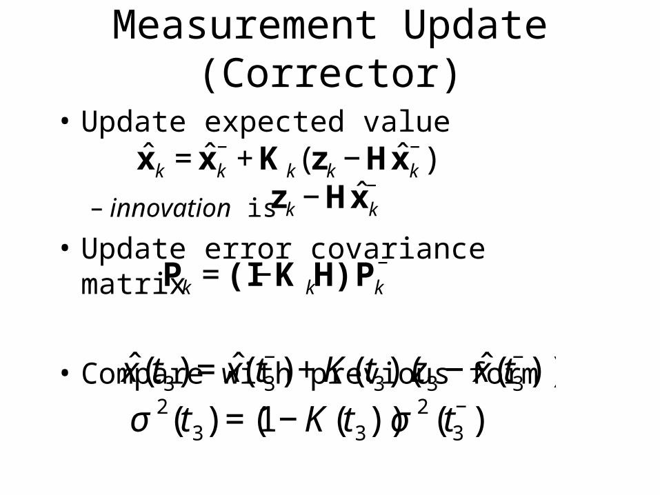
Measurement Update (Corrector)

• Update expected value

– innovation is

• Update error covariance matrix

• Compare with previous form

€

ˆ x k =ˆ x k−+Kk(zk −Hˆ x k

−)

€

zk −Hˆ x k−

€

Pk =(I−K kH)Pk−

€

ˆ x (t3) =ˆ x (t3−)+K(t3)(z3 −ˆ x (t3

−))

€

σ 2(t3) =(1−K(t3))σ2(t3

−)

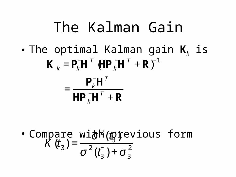
The Kalman Gain

• The optimal Kalman gain Kk is

• Compare with previous form

€

K k =Pk−HT (HPk

−HT +R)−1

€

=Pk

−HT

HPk−HT +R

€

K(t3) =σ 2(t3

−)σ 2(t3

−)+σ32

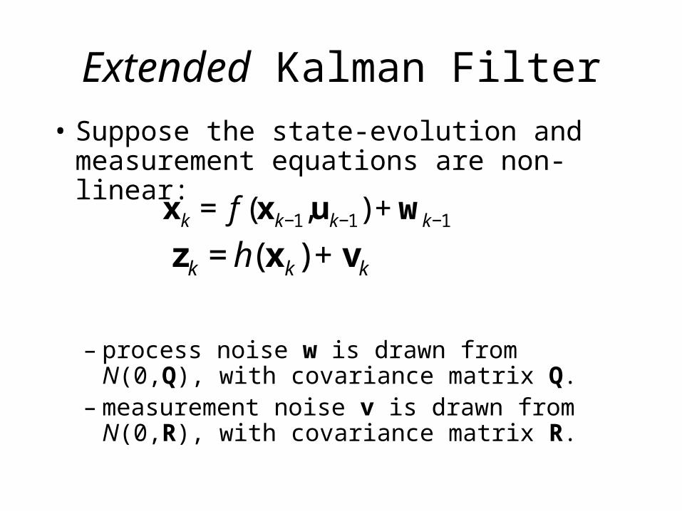
Extended Kalman Filter• Suppose the state-evolution and measurement equations are non-linear:

– process noise w is drawn from N(0,Q), with covariance matrix Q.

– measurement noise v is drawn from N(0,R), with covariance matrix R.

€

x k = f (x k−1,uk−1) + wk−1

€

zk =h(xk)+vk

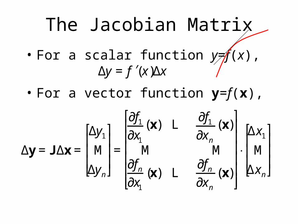
The Jacobian Matrix

• For a scalar function y=f(x),

• For a vector function y=f(x),

€

Δy = ′ f (x)Δx

€

Δy=J Δx=

Δy1

M

Δyn

⎡

⎣

⎢ ⎢ ⎢

⎤

⎦

⎥ ⎥ ⎥ =

∂f1∂x1

(x) L∂f1∂xn

(x)

M M∂fn

∂x1

(x) L∂fn

∂xn

(x)

⎡

⎣

⎢ ⎢ ⎢ ⎢ ⎢ ⎢

⎤

⎦

⎥ ⎥ ⎥ ⎥ ⎥ ⎥

⋅

Δx1

M

Δxn

⎡

⎣

⎢ ⎢ ⎢

⎤

⎦

⎥ ⎥ ⎥

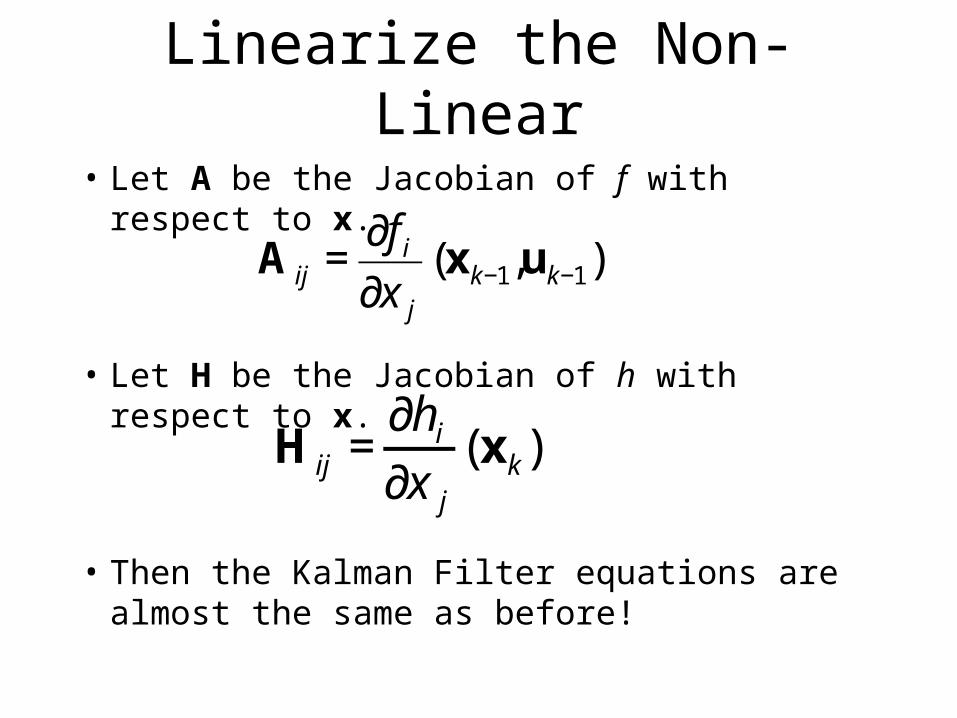
Linearize the Non-Linear

• Let A be the Jacobian of f with respect to x.

• Let H be the Jacobian of h with respect to x.

• Then the Kalman Filter equations are almost the same as before!

€

A ij =∂f i

∂x j

(x k−1,uk−1)

€

Hij =∂hi

∂x j

(xk)

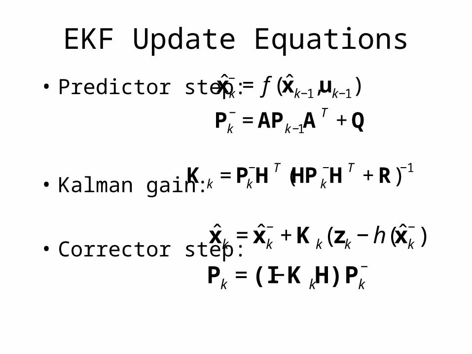
EKF Update Equations

• Predictor step:

• Kalman gain:

• Corrector step:

€

ˆ x k− = f ( ˆ x k−1,uk−1)

€

Pk−=APk−1A

T +Q

€

K k =Pk−HT (HPk

−HT +R)−1

€

ˆ x k =ˆ x k−+Kk(zk −h(ˆ x k

−))

€

Pk =(I−K kH)Pk−