ENDANGERED SPECIES RESEARCHEndang Species Res

Vol. 42: 185–199, 2020https://doi.org/10.3354/esr01048

Published August 20

1. INTRODUCTION

Coastal waters, defined here as the waters be -tween the coastline and the edge of the continentalshelf, are highly productive regions within the global

ocean that support complex marine ecosystems (Ray1988, Sherman 1994). A large proportion of thehuman population lives along the coastline and reliesheavily on coastal waters for a diversity of activities,which makes coastal marine ecosystems particularly

© The authors 2020. Open Access under Creative Commons byAttribution Licence. Use, distribution and reproduction are un -restricted. Authors and original publication must be credited.

Publisher: Inter-Research · www.int-res.com

*Corresponding author: lahuckst@gmail.com

A dynamic approach to estimate the probability ofexposure of marine predators to oil exploration

seismic surveys over continental shelf waters

Luis A. Hückstädt1,*, Lisa K. Schwarz2, Ari S. Friedlaender1, Bruce R. Mate3, Alexandre N. Zerbini4,5,6, Amy Kennedy4, Jooke Robbins7, Nicolas J. Gales8,

Daniel P. Costa1,9

1Institute of Marine Sciences, University of California Santa Cruz, Santa Cruz, CA 95060, USA2Department of Ocean Sciences, University of California Santa Cruz, Santa Cruz, CA 95064, USA

3Marine Mammal Institute, Oregon State University, Newport, OR 97365, USA4Joint Institute for the Study of Atmosphere and Ocean (JISAO),

University of Washington & Marine Mammal Laboratory, NOAA, Seattle, WA 98112, USA5Marine Ecology and Telemetry Research, Seabeck, WA, 98380, USA

6Instituto Aqualie, Juiz de Fora, MG, Brazil7Center for Coastal Studies, Provincetown, MA 02657, USA

8Australian Antarctic Division, Kingston, Tasmania 7050, Australia9Department of Ecology and Evolutionary Biology, University of California Santa Cruz, Santa Cruz, CA 95060, USA

ABSTRACT: The ever-increasing human demand for fossil fuels has resulted in the expansion ofoil exploration efforts to waters over the continental shelf. These waters are largely utilized by acomplex biological community. Large baleen whales, in particular, utilize continental shelf watersas breeding and calving grounds, foraging grounds, and also as migration corridors. We devel-oped a dynamic approach to estimate the likelihood that individuals from different populations ofblue whales Balaenoptera musculus and humpback whales Megaptera novaeangliae could beexposed to idealized, simulated seismic surveys as they move over the continental shelf. Animaltracking data for the different populations were filtered, and behaviors (transit and foraging) wereinferred from the tracks using hidden Markov models. We simulated a range of conditions of expo-sure by having the source of noise affecting a circular area of different radii (5, 25, 50 and 100 km),moving along a gridded transect of 270 and 2500 km2 at a constant speed of 9 km h−1, and startingthe simulated surveys every week of the year. Our approach allowed us to identify the temporalvariability in the susceptibility of the different populations under study, as we ran the simulationsfor an entire year, allowing us to identify periods when the surveys would have an intensifiedeffect on whales. Our results highlight the importance of understanding the behavior and ecologyof individuals in a site-specific context when considering the likelihood of exposure to anthropo-genic disturbances, as the habitat utilization patterns of each population are highly variable.

KEY WORDS: Disturbance · Ocean noise · Blue whale · Humpback whale · Satellite tracking ·Continental shelf

OPENPEN ACCESSCCESS

Endang Species Res 42: 185–199, 2020

vulnerable to anthropogenic pressures (Costanza1999), including pollution, overfishing, anthro po -genic noise and many others (Jackson 2001, Halpernet al. 2008, 2015).

The high demand for fossil fuel (oil and naturalgas), along with the rapid technological advances intheir exploration and extraction, has created a press-ing need to assess the consequences that these activ-ities have on marine ecosystems, particularly in thecontinental shelf region (but see Merrie et al. 2014).Seismic surveys, an important tool for locating under-water petroleum deposits, are sources of high-inten-sity, potentially far-reaching, low-frequency noise inthe ocean (Nowacek et al. 2015, Harwood et al.2016). Furthermore, these activities have expandedinto higher latitudes as polar sea ice retreats. Anunderstanding of whether and how marine seismicsurveys affect different levels of biological organiza-tion, from individuals to ecosystems, is therefore war-ranted (Nowacek et al. 2015).

Much of the research on the effects of human-generated noise on aquatic organisms has focused onmarine mammals (National Research 2003, Madsen2005), as they have the most sensitive hearing and thebroadest hearing range, and because they directlyoverlap a number of sound-generating activities suchas navy sonar, shipping and seismic surveys. Marinemammals are also protected under the legislations ofseveral countries. To that end, a series of workinggroups developed a conceptual framework (popula-tion consequences of disturbance [PCoD] model) toaddress how human-caused disturbances in marinemammals (acute or chronic) link to changes in pop -ulation growth (Fig. S1 in the Supplement at www.int-res. com/ articles/ suppl/ n042 p185 _ supp. pdf) (Na-tional Research Council 2005, New et al. 2013, 2014,Harwood et al. 2016, National Academies of Sciences,Engineering, and Medicine 2017, Pirotta et al. 2018).

Ongoing efforts continue to improve our under-standing of the model’s transfer functions (mecha-nisms connecting exposure to a disturbance tochanges in behavior, life function, vital rates andpopulation dynamics; see National Research Council2005, New et al. 2013), particularly with respect tothe effects of lost foraging time as a result of distur-bance (Goldbogen et al. 2013, King et al. 2015, Fried-laender et al. 2016). The most recent iteration of theframework (population consequences of multiplestressors [PCoMS] model) includes the likelihood ofexposure as an important early step. The aforemen-tioned probability, however, has traditionally beenestimated employing a static approach using sourcesof disturbance fixed both in space and time (e.g.

Maxwell et al. 2013, Costa et al. 2016b, Ellison et al.2016). Al though informative, those approachesignore the dynamic nature of an animal’s behavioraland movement patterns (i.e. animals are not persist-ently occupying their entire range), as well as spa-tially and temporally dynamic sources of disturbance(e.g. military operations or seismic surveys). A morethorough understanding of exposure can be obtainedby using an approach that incorporates animal move-ment and a dynamic source of disturbance (Costa etal. 2016a, Ellison et al. 2016).

Rorquals (family Balaenopteridae), which includethe largest species of animals ever to have lived on theplanet, inhabit all oceans of the world, typically breedin low latitudes and migrate to coastal highly produc-tive, mid- and high-latitude regions to forage. Rorqualpopulations were severely depleted by human har-vesting, but with the end of whaling during the secondhalf of the 20th century, many populations are now re-covering (Clapham et al. 1999, Thomas et al. 2016).

Some rorquals use the continental shelf waters forboth migration and foraging, and are thus likely tocome into conflict with human activities, particularlyas a result of exposure to sources of intense, mid- tolow-frequency noise (Southall et al. 2012). Further-more, ocean noise is particularly relevant to rorqualsas they rely heavily on sound for important aspects oftheir biology (Harwood 2001, Van der Hoop et al.2013, Nowacek et al. 2015, Thomas et al. 2016). In-deed, an important effort has been directed to wardsenhancing our understanding of how noise ex posureelicits changes in the behavior of individuals (behav-ioral response studies) (Southall et al. 2012, 2016,Goldbogen et al. 2013, Friedlaender et al. 2016).

Because of their large size, high energetic de -mands and life histories, rorquals range over broad,basin-wide areas, and thus the likelihood of theirexposure to a disturbance will vary in both space andtime. In this study, we used animal movement datacollected from different populations of blue (Bala eno -ptera musculus) and humpback whales (Mega pteranova engliae) across the globe to estimate whetherand for how long individuals from a populationwould be exposed to a series of simulated, idealizedseismic surveys, assuming the exposure does notelicit any behavioral modifications. Our model pro-vides a data-derived empirical view of how a movingsource of disturbance could impact individuals asthey move throughout their environment, whichallows us to describe the spatial and temporal vari-ability in the potential impacts of seismic surveys atthe individual (behavioral state) level as well as theproportion of individuals affected.

186

Hückstädt et al.: Simulated exposure to seismic surveys

2. MATERIALS AND METHODS

2.1. Animal movement data

We compiled movement data for blue and hump-back whales from 8 areas of the world, represent-ing 2 and 6 distinct populations of blue and hump-back whales, respectively (Table 1, Fig. 1). Someof these data sets have been analyzed and pub-lished elsewhere (Zerbini et al. 2006, 2011, Baileyet al. 2009, de Castro et al. 2014, Irvine et al. 2014,Kennedy et al. 2014, Weinstein et al. 2018). These

areas were chosen based on the availability of ani-mal tracking data, rather than their likelihood ofbeing subject to actual surveys, as the purpose ofthis initial modeling exercise was to incorporate adynamic approach and apply it to species of differ-ent behavior, rather than to address the potentialof exposure in specific areas. In this study, wedefine exposure as the overlap, in space and time,between the location of a particular individualand a circle of determined radius representing thearea affected by the simulated seismic survey (seeFig. 2 and Section 2.2).

187

Species Site N Days Time over shelf % HR % LR transmitting waters (%)

Blue whale California Current 104 6−504 20.3 83.6 16.4 Western Australia 10 7−179 9.7 76.5 23.5

Humpback whale Bering Sea 8 9−94 66.2 56.9 43.1 California Current 12 3−122 51.1 31.2 68.8 Antarctic Peninsula 24a 5−210 77.3 89.3 10.7 Gulf of Maine 55 2−112 96.7 68.9 31.1 Southwest Atlantic 12 8−284 14.2 84.6 15.4 Eastern Australia 30 3−154 23.6 65.8 34.2

aData limited to 500 km from the break of Antarctic continental shelf

Table 1. Movement data summaries for blue and humpback whale tracking data sets included in the study. HR: high residence behavior; LR: low residence behavior

Humpback whale

Blue whale

25000 5000 10 000 km

6

3

1 5

2

7

4

Fig. 1. Individual tracks of blue whales (yellow) and humpback whales (purple) included in this study. The numbers on the mapcorrespond to the different regions. Blue whale tracking data sets were collected in the California Current (1: CalCur, n = 104) andWestern Australia (2: WesAus, n = 10). Humpback whale tracking data sets were collected in the Bering Sea (3: BerSea, n = 8),California Current (1: CalCur, n = 12), Antarctic Peninsula (4: AntPen, n = 24), Gulf of Maine (5: GulMai, n = 55), Southwest

Atlantic (6: SouAtl, n = 12) and Eastern Australia (7: EasAus, n = 30)

Endang Species Res 42: 185–199, 2020

Animal tracking data were collected and transmit-ted using the Argos satellite system (Toulousse,France). All raw tracking data were analyzed in R3.1 (R Development Core Team 2019). First, datawere pre-processed using a speed filter to removeevident erroneous positions (McConnell et al. 1992)and later processed with a continuous-time corre-lated random walk model (crawl R package) (John-son et al. 2008) to render realistic estimates of ani-mal movement at regular time intervals that variedby data set based on the quality of the data sets anddata gaps. As the tracking data were collected overmany different years and our goal was to build sim-ulations for a period of 1 yr, all tracks were stan-dardized to a common single year by converting tocalendar day (1−365 d). As diving depth data werenot available and to avoid the complications associ-ated with modeling noise propagation in 3 dimen-sions (see Section 2.2), we did not consider depth inour modeling approach.

Given that the PCoD/PCoMs model focuses onchanges in time−energy budget with respect to lostforaging time, it was necessary to infer behavioralstates from the animal movement data. This wasdone by processing the crawl-processed trackingdata through hidden Markov models (HMMs) to de -fine behaviors (high residency, HR, or low residency,LR) using the package momentuHMM in R (McClin-tock et al. 2018). The HR behavior was characterizedas sections of the tracks where animals displayed aslow transit rate and high turning rate (high tortuos-ity), remaining in a particular area for a prolongedamount of time (i.e. foraging or breeding, dependingon the area). LR behavior, in contrast, was character-ized as sections of the track where animals swamfaster and with a clear directionality.

2.2. Simulations of seismic surveys

Given the variability in the spectrum of transectsizes and conformation of seismic surveys, we optedto define 2 types of idealized survey transect: (1) 3Dsurvey: 85 parallel transect lines of 50 km in length,spaced every 600 m; and (2) 4D survey: 100 paralleltransect lines of 20 km in length, spaced every 200 m(Fig. 2). These surveys are based on the general char-acteristics of a ‘typical seismic survey’ and capturethe basic movement patterns of seismic vessels, mak-ing them a realistic generic approximation of thepotential of exposure. Real seismic exploration 3Dsurveys acquire data on a 3D grid, allowing horizon-tal projections in directions other than along the tran-

sects, whereas 4D surveys can acquire the same dataas 3D surveys adding the time dimension, shootingthe same grid at regular intervals, allowing the gen-eration of time series. For each population includedin the study, we randomly placed 100 surveys of eachtype over the continental shelf waters that were uti-lized by the whales (as identified from kernel homerange analysis).

Due to the inherent complexity of sound propaga-tion for different ocean basins and continental mar-gins, and the need to come up with general patternsthat could be applied to a variety of environments,we chose to simulate the area of exposure as a hori-zontal circle of different radii (5, 25, 50 and 100 km),as these radii encompass the most reasonable rangeof distances that could elicit a behavioral response byanimals to seismic surveys (Nowacek et al. 2015)(Fig. 2). These simulated sources moved along thegrid at a constant speed of 9 km h−1 (ca. 4.5 − 5 knots),accounting for a lag of 3 h when switching surveylines when no sound emissions were active. To incor-porate the temporal variability in the tracking dataand movement patterns of the individuals, we set thefirst day of every week of the year (i.e. 52) as the starttime for every combination of survey and radius.Therefore, for each population, we had a total of 100surveys × 2 survey types × 4 radii of exposure × 52 wk,totaling 41 600 simulations.

Finally, all animal movement data were interpo-lated at a regular time interval (1 h) and the spatialoverlap between the area of influence of the simu-lated survey and the animals’ location was calcu-lated. From this overlap, we were able to calculatethe proportion of the tagged individuals exposed, thetotal time each individual was exposed, and theamount of exposure time for each behavior.

Each one of these variables was estimated forstandardized periods of 1 wk, obtaining (1) the pro-portion of the tagged individuals under exposureper week; (2) the number of animal hours of expo-sure per week (maximum 168 h); (3) the number ofanimal exposure hours in LR behavioral state perweek (maximum 168 h); and (4) the number of ani-mal ex posure hours in HR behavioral state perweek (maximum 168 h).

3. RESULTS

We ran a total of 41 600 possible combinations ofsurveys (4D and 3D) and radii of exposure (5, 25, 50and 100 km) for 2 populations of blue whales and 6populations of humpback whales.

188

Hückstädt et al.: Simulated exposure to seismic surveys 189

step angle

Raw Argos tracking data

crawl

momentuHMM

1. Track processing

Filtered tracks with behavior (high residence [green]and low residence [purple])

Randomly placed on utilized shelf waters

2. Survey design

10 km

× 100

3D 4D

100 km 50 km 25 km 5 km3. Spatial and temporal variability of disturbance

Survey start (calendar day) 1, 8, 15, 22, ..., 348

Week 1 Week 52

4. Exposure at the individual and tagged population level

∑ Time under exposure

Nind

5 10 15 20 25 30 35 40 45 50

102030405060708090

100

Surv

ey

WeekFig. 2. Simulation approach used to estimate the probability and duration of exposure to seismic surveys across differentpopulations of blue (N = 2) and humpback whales (N = 6). In Step 3, red lines show transects and yellow ovals show expo-sure radii. In Step 4, sigma corresponds to the sum of time across individuals; the colors refer to exposure intensity or the

mean individual time under exposure (see Fig. 5), with warmer colors indicating longer exposures

Endang Species Res 42: 185–199, 2020

3.1. Movement patterns

There were clear differences in the patterns ofmovement and habitat utilization among populations.As reported previously, blue whales (California Cur-rent and Western Australia) spent the majority of theirtime off the continental shelf (Fig. 1 and Table 1) (Bai-ley et al. 2009, Double et al. 2014, Irvine et al. 2014).However, the time spent on the continental shelf waspredominantly identified as HR behavior, likely indi-cating that they were foraging in those waters.

While most of the humpback whales were taggedon their foraging grounds (Bering Sea, California Cur-rent, Antarctic Peninsula, and the Gulf of Maine),individuals from 2 populations (Southwest Atlanticand Eastern Australia) were tagged at their low-lati-tude breeding grounds or along their transit towardstheir high-latitude foraging grounds (Table 1, Fig. 1).As expected, individuals migrating across oceanbasins spent the least amount of the time over con -tinental shelves (14.2 and 23.6% for individuals fromthe Southwest Atlantic and Eastern Australian popu-lations, respectively; Table 1). The remaining hump-back whale populations ex hibited a pattern that waslargely associated with waters over continental shelves,or close to the continental shelf break (e.g. CaliforniaCurrent) (Fig. 1). Tracking data for some individualstagged in the Antarctic Peninsula were sufficientlylong to record their migration to breeding grounds inthe Eastern Equatorial Pacific. For this population, werestricted the analysis to areas within 500 km of theedge of the Antarctic continental shelf.

3.2. Behavioral states

The behavioral categorization using HMMsshowed similarity in the movements within species.Most data sets presented a clear distinction betweenthe 2 defined behaviors (HR and LR), although bluewhales off the California Current system departedfrom this binary definition of behaviors and showedinstead a more complex scenario, with more plausi-ble solutions of the HMMs distinguishing at least 3behaviors (not shown here). Yet, since our aim was tocompare across the different populations rather thananalyze the movement and behavioral patterns ofeach population, we opted to use the 2-behavioralstates output for consistency across the study sites.

With the exception of humpback whales in the Cal-ifornia Current, all whales spent the majority of theirtime over continental shelf waters engaged in HRbehavior (56.9−89.3%) (Table 1).

3.3. Simulated exposures

The number of randomly placed surveys that im -plied exposure to the different populations of whalesvaried widely across populations, with a minimum often 4D surveys with a radius of 5 km for the bluewhales from Western Australia, and a maximum of100 3D surveys with a radius of 100 km for the hump-back whales tagged in the Bering Sea.

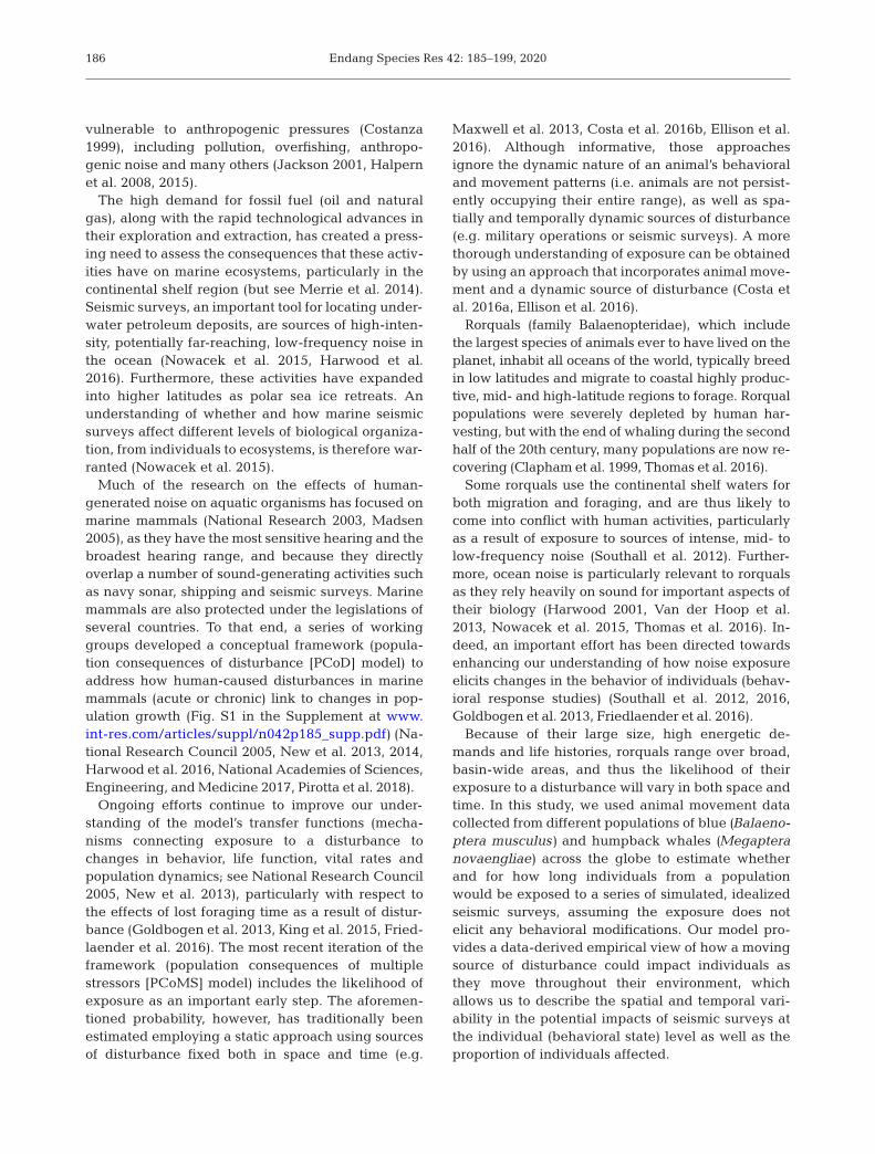
3.4. Proportion of individuals experiencing exposure

The proportion of the tagged individuals that over-lapped with seismic surveys varied widely across thespecies and sites. Irrespective of the survey type orthe radius of influence, the probability of exposure forblue whales in the California Current and humpbackwhales off both the Antarctic Peninsula and EasternAustralia was consistently low (75th percentile <0.13). In contrast, humpback whales from the BeringSea consistently exhibited the highest proportion oftracks overlapping with seismic surveys (25th per-centile = 0.31, 75th percentile = 0.81), followed byhumpback whales in the California Current (Fig. 3).

Despite the differences in the area and duration ofexposure between 4D and 3D surveys, the proportionof tagged individuals that were affected did not differ

190

0 0.1 0.2 0.3 0.4 0.5 0.6 0.7 0.8 0.9 1

WesAus

EasAus

BerSea

AntPen

GulMai

CalCur

CalCur

SouAtl

Proportion of tagged individuals exposed

Fig. 3. Proportion of the tagged individuals of blue whales(yellow) and humpback whales (purple) exposed to simu-lated seismic survey per site (for site abbreviations, see Fig. 1legend). Data for all combinations of survey design (4D and3D) and radii of influence (5, 25, 50 and 100 km) were pooledtogether. The white line represents the median. The edges ofthe boxes represent the 25th and 75th percentiles, and the

lines represent the 5th and 95th percentiles

Hückstädt et al.: Simulated exposure to seismic surveys

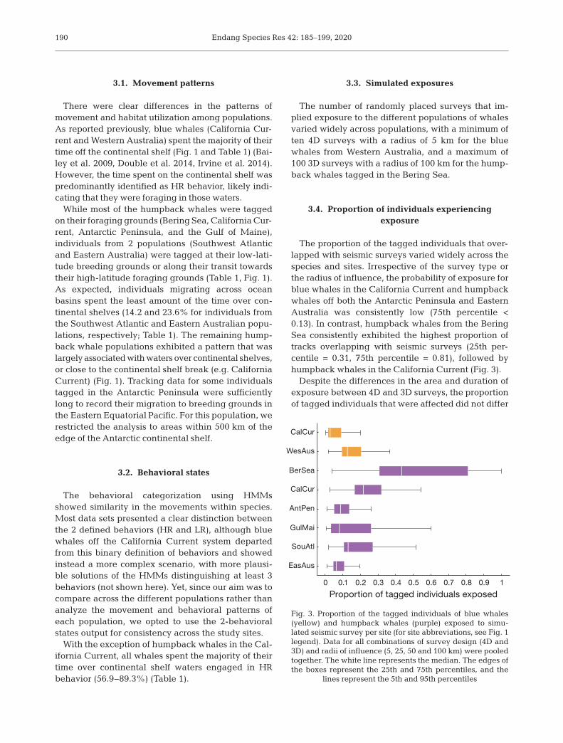
greatly between the survey designs (Fig. 4). Therewere, however, differences in the effect of increasingradii of influence across sites. For instance, themedian probability of exposure for humpbackwhales from Eastern Australia with 3D surveys onlyin creased from 0.02 to 0.09 for a 5 and 100 km radius,

respectively. In contrast, the sameincrease in the radius of exposure forhumpback whales from the BeringSea resulted in an increase in themedian probability from 0.22 to 0.71(Fig. 4).

3.5. Individual time and behaviorunder exposure

We calculated the mean individualduration (h wk−1) of the simulated expo-sure affecting each be havioral state(HR or LR), an indicator of the worst-case possible scenario as we assumedthat whales do not leave the affectedarea (Table 2). When all possible com-binations of surveys and radii are in-cluded in the analysis, blue whalesfrom Western Australia had the short-est mean individual exposure to thesimulated seismic surveys (median =11.71 h wk−1), followed by humpbackwhales off Eastern Australia (median =22.33 h wk−1) and humpback whalesfrom the South Atlantic (median =22.50 h wk−1). Surprisingly, increasingthe radius of influence to 25 km im-

plied, across all data sets, a dramatic rise in the meanindividual time animals were exposed for both behav-iors (HR and LR) when compared to a 5-km radius,even for areas whose tracks indicated low ex posureproportions (Table 2). For instance, humpback whalesfrom the South Atlantic went from being exposed

191

4D 3D 5 km 25 km 50 km 100 km 5 km 25 km 50 km 100 km

Blue whaleCalifornia Current 42 37 82 82 82 82 82 82 37 34 122 117 126 125 126 126Western Australia 5 5 15 15 48 33 89 68 6 6 62 54 112 94 124 124

Humpback whaleBering Sea 43 25 91 55 92 74 92 81 27 17 124 78 126 93 126 112California Current 30 11 82 49 83 71 83 81 22 8 118 60 126 97 126 126Antarctic Peninsula 18 18 90 90 92 92 93 93 26 23 121 113 126 125 126 125Gulf of Maine 60 48 98 94 98 95 98 94 76 61 126 108 126 123 126 123South Atlantic 12 12 76 76 92 92 92 92 17 16 117 117 125 125 126 126Eastern Australia 23 23 89 88 89 89 91 90 15 12 110 99 124 120 126 124

Table 2. Maximum number of hours of individual exposure to simulated seismic surveys (4D and 3D) across the range of blueand humpback whales. The radii of exposure considered were 5, 25, 50 and 100 km. Grey cells indicate high residence (HR)

behavior. White cells indicate low residence (LR) behavior

WesAus

EasAus

BerSea

AntPen

CalCur

CalCur

SouAtl

GulMai

0 1 00.5 0.5 1

100 km50 km

25 km 5 km

100 km 50 km

25 km 5 km

4D 3D

Proportion of tagged individuals exposed

Fig. 4. Proportion of the tagged individuals of blue whales (yellow) and hump-back whales (purple) exposed to simulated seismic survey per site (for site ab-breviations, see Fig. 1 legend), survey and radius of influence. The white linerepresents the median. The numbers beside the bars (shown for CalCur) cor-respond to the different radii of influence used in the simulations. The edges ofthe boxes represent the 25th and 75th percentiles, and the lines represent the

5th and 95th percentiles

Endang Species Res 42: 185–199, 2020

12 h wk−1 in HR behavior under a 5-km 4D survey to76 h wk−1 in HR behavior under a 25-km 4D survey(Table 2). The magnitude of these increases is similarfor all data sets.

3.6. Cumulative exposure

To better assess the effect of simulated exposure toseismic surveys, we can evaluate the relationshipbetween the proportion of tagged individuals andmean individual time under exposure under everypossible combination of survey design and radii of in -fluence (Fig. 2). We observed 2 general patterns thatare more easily described using the most ex tremecases for each: blue whales in the California Currentand humpback whales from the Bering Sea (Fig. 4).We did not find a relationship be tween the propor-tion of individuals exposed and the mean individualtime that animals were exposed. Instead, across thedifferent radii, we saw very high proportions of indi-viduals under exposure and rather short exposures,whereas the longest exposures (>60 h wk−1) corre-spond to proportions in the 0.3−0.6 range (Figs. 4 &5). Blue whales from the California Current, in con-trast, did not generally show an increase in the pro-portion of tagged individuals exposed beyond 0.4,regardless of the survey design, and increasing theradii or the area affected (4D versus 3D) did increasethe mean individual exposure time but not the pro-portion of individuals affected (Figs. 4 & 5).

3.7. Spatio-temporal patterns of disturbance

By using a dynamic approach to estimate the prob-ability of exposure to a disturbance under severalscenarios, we can illustrate the spatial and temporalvariability of exposure probability, and can then de -termine areas and times of enhanced susceptibility toimpacts from hypothetical seismic surveys for differ-ent populations. For instance, our simulations indi-cated that, regardless of the radius of influence,humpback whales from Eastern Australia were con-sistently exposed to the simulated seismic surveys forthe shortest amount of time across all sites (Fig. 5),and this held true regardless of when in the year thesurvey took place. On the other hand, there is a sev-eral week period during which humpback whalesfrom the Gulf of Maine were exposed for prolongedperiods (Fig. 5).

Finally, given the spatially explicit nature of ourapproach, it would be possible to determine areas

of higher susceptibility to disturbances across therange of a given population (Fig. S2). Humpbackwhales from the Bering Sea had no clear spatialpattern of susceptibility across their range, both interms of probability of exposure as well as time(and time in HR behavior) under exposure (Fig. S2).Blue whales from the California Current, in con-trast, clearly present a heterogeneous spatial pat-tern, with areas where the susceptibility to seismicsurveys increases either in terms of probability ofexposure, mean individual time of exposure, orboth (Fig. S2).

4. DISCUSSION

Underwater noise can have deleterious effects onmany marine animals, an issue of particular relevanceto marine mammals due, among other things, to theirreliance on acoustics to communicate among con-specifics, locate food and navigate (Myrberg 1990,National Research Council 2003, 2005, Erbe 2012,Nowacek et al. 2015, Costa et al. 2016a, Ellison et al.2016). Regardless of the consequences that exposureto seismic surveys might have on large whales (e.g.behavioral, and physiological responses), key compo-nents of understanding the effects of anthropogenicactivities on these populations are realistic estimatesof the encounter rate and interaction duration.

The PCoD/PCoMS framework provides an ap -proach to describe how (acoustic) disturbances mightaffect marine mammals (National Research Council2003, New et al. 2013, King et al. 2015, Costa et al.2016a, Harwood et al. 2016), and although significantcontributions have been made to define the transferfunctions and parameters of the PCoD/PCoMSmodel, the spatial and temporal overlap between dis-turbance and animals (i.e. potential of exposure) hasremained less explored (Costa et al. 2016a, Ellison etal. 2016). Our study provides a general assessment ofthe likelihood or probability of blue and humpbackwhales being exposed to a seismic survey in theirhabitat on the continental shelf, and of how that like-lihood varies depending on both the behavior of thespecies and the radius of influence that may elicit aresponse. Furthermore, as we empirically estimatebehavioral states from the tracking data to calculatethe likelihood of exposure, we demonstrate that evenin areas of lower time spent by the whales (i.e. LRbehavior), seismic surveys have the potential toimpact individual whales for periods similar to thoseseen in areas of higher usage (i.e. HR behavior).While the impacts of the exposure under different

192

Hückstädt et al.: Simulated exposure to seismic surveys 193

Cal

Cur

Wes

Aus

BerS

eaCal

Cur

AntP

enG

ulMai

SouA

tlEa

sAus

A 5 km 25 km 50 km 100 km

5 50

20

40

60

80

100

120

Tim

e ex

pose

d pe

r ani

mal

(h w

k–1)

Week of the year (1–52) versus survey number

Fig. 5. Variability in mean individual time exposed (h wk−1) to simulated seismic surveys for blue and humpback whales acrossone year for (A) 4D and (B) 3D surveys. Each panel corresponds to a different radius of influence (5, 25, 50 and 100 km).Warmer colors indicate longer exposures, with a possible maximum of 126 h wk−1. For site abbreviations, see Fig. 1 legend

Figure continued on next page

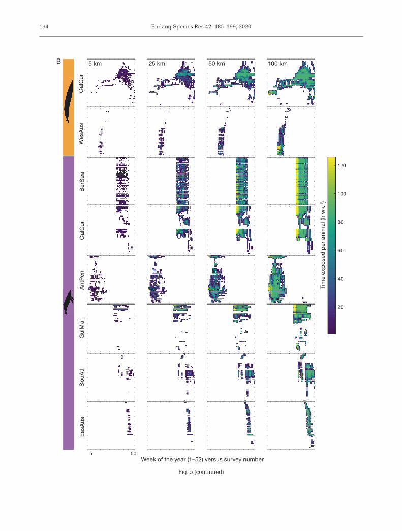
Endang Species Res 42: 185–199, 2020194

Cal

Cur

Wes

Aus

BerS

eaCal

Cur

AntP

enG

ulMai

SouA

tlEa

sAus

B 5 km 25 km 50 km 100 km

Tim

e ex

pose

d pe

r ani

mal

(h w

k–1)

5 50Week of the year (1–52) versus survey number

20

40

60

80

100

120

Fig. 5 (continued)

Hückstädt et al.: Simulated exposure to seismic surveys

behaviors are yet to be determined, it is evident thatwe need to consider the effects of disturbancesbeyond the traditional view that has focused on highusage areas (Costa et al. 2016a, Ellison et al. 2016,Guerrini et al. 2019).

A fully implemented seismic survey usually oper-ates an array of air guns that produce noise every1−15 s, at a source spectral level that ranges between1 and 100 Hz of about 205−255 dB re. 1 μPa at 1 m(Myrberg 1990, Nowacek et al. 2015). Regardless ofthe dimensions of the survey (4D or 3D for this study,see Section 2), the source of noise can affect an areaduring a period of weeks. Thus, the temporal andspatial scales of such sources of disturbance matchthe scale over which a wide diversity of large andmedium-sized marine vertebrates operate. In thisstudy, we take an alternative approach and departfrom studies that focus on highly resident species ofrestricted range, such as harbor porpoises Phocoenaphocoena and harbor seals Phoca vitulina (Myrberg1990, Harwood 2001, Bain & Williams 2006, Tougaardet al. 2009), and instead estimate the exposure risk forseveral populations of 2 species of large migratorywhales.

Both blue and humpback whales have a well-known annual life history, breeding in low latitudesand then migrating to mid- and high-latitude highlyproductive coastal areas to forage, which will influ-ence their potential exposure to disturbance (Costaet al. 2016a). Despite the differences in their move-ment patterns, we found that, when affected, mostindividuals in our study had probabilities of exposurethat ranged between 0.02 and 0.32, depending onthe population in question (Tables 1 and 2, Figs. 3, 4and 6). Humpback whales from the Bering Sea,where the data only included movements at foraginggrounds, were the exception, having the most con-strained distribution across data sets and exposureprobabilities that clustered in the 0.31 and 0.81 range(25th and 75th quartiles) (Fig. 3).

Several studies have suggested that seismic surveyair gun noise does not elicit a behavioral responsefrom large baleen whales (e.g. cause them to leavethe area) unless individuals are within 15−20 km ofthe source (Myrberg 1990, McDonald et al. 1995, Mc-Cauley et al. 2000), although their acoustic be havioris likely affected at longer distances (Di Iorio & Clark2009, Cerchio et al. 2014). By using empirical tracksof individuals along with realistic seismic survey sce-narios, our methods provide the next step in realisti-cally determining the overlap be tween surveys andseveral whale populations. However, our methodsonly provide an estimate for the maximum amount of

exposure since we did not account for animals mov-ing away from the sound source. Future efforts couldincrease complexity by integrating sound source−animal overlap with dose− response curves (probabil-ity of moving away from a sound and the distancetraveled) to determine actual lost foraging time(Table 2). Across the different data sets used in thisstudy, blue whales from western Australia wereunique in their relatively low duration of exposure toseismic surveys, if we consider radii of influence of 5and 25 km (Table 2). Perhaps more interestingly,however, is the fact that for all other populations, aradius of 25 km was enough to expose individualwhales at a near-maximum duration (126 h), withonly a marginal increase in the maximum duration ofthe exposure if the radius is increased to 50 or 100 km(Table 2).

To better visualize the potential effect of seismicsurveys on the different populations of whales, weanalyzed the relationship between time spent in HRunder exposure versus the probability of the popula-tion being affected by the different surveys (Fig. 6).The area and shape of the minimum convex polygons(MCPs) for these plots can be used as an indicator ofthe potential impact for each population.

At one end of the spectrum, blue whales from west-ern Australia showed a clear effect of the survey de-sign and radius of influence on the impact of the sur-veys. As the radius increases, so does the potentialeffect of the survey, and 3D surveys (the largest)caused longer maximum exposures to the seismicsurveys (Fig. 6C,D). At the other end of the spectrum,highly restricted humpback whales from the BeringSea showed MCPs elongated along the y-axis (pro-portion of tagged individuals disturbed), indicatingthat even small radii (5 and 25 km) have thepossibility to affect most of the population (>0.6)(Fig. 6E,F). Indeed, 100% of the Bering Sea whalescould be exposed for as long as 50 h (Fig. 6F). Inter-estingly, humpback whales off the Gulf of Maine, thesecond most restricted in terms of their movementpatterns, only had an elevated potential of exposureto seismic surveys for the largest radii (50 and100 km) (Fig. 6K,L). The differences among the dif-ferent data sets included in our study are likely asso-ciated with a combination of factors, from the spatialspread in the surveys due to the different extension ofthe continental shelf habitat utilized by each popula-tion, to differences in the behavior of individualsamong populations. For instance, humpback whalesin the Bering Sea had one of the smallest homeranges across data sets and yet most individuals dis-played similar patterns of habitat utilization, which

195

Endang Species Res 42: 185–199, 2020196

0 60 1200

15 km25 km50 km100 km

A B

Cal

Cur

Cal

Cur

BerS

ea

Wes

Aus

AntP

enG

ulM

aiSo

uAtl

EasA

us

C D

E F

G H

I J

K L

M N

O P

4D Surveys 3D Surveys 4D Surveys 3D Surveys

Foraging time under exposure per week (h)

Prop

ortio

n of

pop

ulat

ion

dist

urbe

d

Fig. 6. Potential impacts of simulated surveys for blue whales(yellow) and humpback whales (purple) illustrated as the re-lationship between the proportion of the tagged individualsexposed and the time under exposure in high residence (HR)behavior. Each dot corresponds to a specific transect−weekof the year combination, and the dashed lines represent theminimum convex polygon, indicating the total range of po-tential impacts. The tones of blue represent the radius of in-fluence, with the lightest blue representing 5 km and thedarkest corresponding to 100 km. Left panels (A, C, E, G, I, K,M and O) correspond to the smaller 4D surveys. Right panels(B, D, F, H, J, L, N and P) correspond to the larger 3D surveys.

For site abbreviations, see Fig. 1 legend

Hückstädt et al.: Simulated exposure to seismic surveys

likely drove the elevated impacts observed for thisdata set. Additionally, differences in sample size canalso influence these results.

To assess the effects of anthropogenic noise onmarine animals, it is necessary to have informationavailable at the appropriate time and spatial scales(Myr berg 1990). Consequently, the PCoD/PCoMSframework requires spatially explicit information onthe abundance and distribution of marine mammalsand how these are linked to individual behavioralresponses (Bailey et al. 2014, Costa et al. 2016a, Har-wood et al. 2016). Furthermore, there is an urgentneed to better anticipate the impact of anthropogenicactivities and to understand how susceptibility ofparticular populations varies across space and time.

While our analysis is a basic exercise based on sim-ulated surveys and assumes that whales do not altertheir behavior, our results highlight the importanceof understanding the behavior and ecology of indi-viduals in a site-specific context when consideringthe likelihood of exposure to anthropogenic distur-bances. For instance, our approach allowed us toidentify the temporal variability in the susceptibilityof the different populations under study, as we ranthe simulations for an entire year, enabling us toidentify periods when the surveys would have an in-tensified effect on whales (warmer colors, Fig. 5A,B).This, however, is invariably a function of the samplesize and length of the tracking data set. Blue whalesin the California Current had the largest and longestdata set, allowing us to robustly detect variations inthe susceptibility across the range of the populationand almost for a full year, whereas the Bering Sea orEastern Australia humpback whales data sets offer alimited glimpse of the potential impacts of seismicsurveys (Fig. 5A,B, Fig. S2). If we aim at understand-ing how human activities can potentially affect dif-ferent populations of marine animals, we need amore complete picture of their movement patternsacross an entire annual cycle (i.e. larger and longertracking data sets).

Traditionally, data on the range, abundance anddistribution of species that are being exposed to asource of noise have been collected using visual sur-veys (Bailey et al. 2014). While these data are valu-able and can be very informative to discern behav-ioral responses of animals under exposure, there areintrinsic biases that limit the application of surveydata (e.g. detection probability, spatial range of theobservations, and transect design, among others)(Palka & Hammond 2001, Hammond et al. 2002,Bombosch et al. 2014). Tracking data, in contrast,have the potential to provide unbiased information

about the movement patterns of animals at muchlonger scales and over prolonged periods. Further-more, the development of new statistical tools nowallows us to infer behavioral stages from trackingdata (Jonsen et al. 2005, Michelot et al. 2017,McClintock & Michelot 2018), giving us the ability tolink habitat usage with at-sea behavior.

Similarly to seismic surveys, other anthropogenicstressors in the oceans (e.g. shipping, fishing, recre-ational boating) are dynamic in space and time (Weil-gart 2007, Gomez et al. 2016). There is also anincreasing pressure to consider temporal changes inthe ocean’s conditions and human activities to imple-ment better protection measures (Hyrenbach et al.2000, Maxwell et al. 2015). Our modeling approachcan easily be adjusted to be applied to real-worldscenarios where there is a need to evaluate the im -pact of other sources of noise or to assess the effec-tiveness of mitigation measurements (e.g. postpon-ing a survey, reducing the number of transect lines,or moving a shipping route offshore). The strength ofthis approach lies in the fact that it acknowledgesthat the sources of exposure, as well as the animals,are dynamic, making it a more realistic way to under-stand how anthropogenic activities could affect natu-ral populations of marine animals, and how protec-tion can be implemented. Future iterations shouldalso consider the possibility of combining the likeli-hood of exposure, as defined in this study, withdynamic species modeling forecasts similar to toolsalready available to minimize fisheries interactions(Hazen et al. 2018). This would provide near real-time predictions of occurrence, given particular envi-ronmental covariates, along with a context-specificassessment of the likelihood of exposure at relevantspatial and temporal scales, improving our ability tominimize the impact of seismic surveys.

We demonstrate that, by using tracking data, wecan estimate the maximum likelihood of exposure tosimulated moving sources of disturbance, providingus with an estimate of (1) the proportion of individu-als that would be exposed, (2) the time for whichindividuals would be exposed and (3) the behavioraffected by the disturbance. This information is a piv-otal first step (Fig. S1) toward evaluating population-level impacts of a disturbance. These results can thenbe used (along with data from behavioral responsestudies, metabolic rate prey availability studies,among others) to estimate the costs of that distur-bance on an individual’s energy budget, includingthe amount of energy expended but not acquired, theadditional time an individual would have to spendforaging to offset this lost foraging time, and the sub-

197

Endang Species Res 42: 185–199, 2020

sequent effects on offspring growth and survival(National Research Council 2003, New et al. 2013,Costa et al. 2016a,b).

Acknowledgements. This work was developed in associa-tion with the Office of Naval Research-supported PCAD/PCOD working group and was supported by Office of NavalResearch grant N00014-08-1-1195, and the E&P Sound andMarine Life Joint Industry Project of the International Asso-ciation of Oil and Gas Producers (JIP 00 07-23). Taggingresearch in the Gulf of Maine was supported by the NationalOceanographic and Atmospheric Administration andExxonMobile Exploration Company via the National Fishand Wildlife Foundation and the National OceanographicPartnership Program. Tagging research of blue and hump-back whales in the California Current was supported in partby the Tagging of Pacific Pelagics, Office of Naval Research(grant N00014-09-1-0453) and donors to Oregon State Uni-versity Endowments for Marine Mammal Research and theMarine Mammal Institute. Tagging in the western SouthAtlantic was funded by Shell Brasil with grants provided toBiodinâmica and Instituto Aqualie. Tagging in the BeringSea was funded by the former Minerals Management Serv-ice (now Bureau of Ocean Energy Management) with grantsto the Marine Mammal Laboratory, Alaska Fisheries ScienceCenter. The scientific results and conclusions, as well as anyviews or opinions expressed herein, are those of theauthor(s) and do not necessarily reflect those of NOAA orthe US Department of Commerce.

LITERATURE CITED

Bailey H, Mate BR, Palacios DM, Irvine L, Bograd SJ, CostaDP (2009) Behavioural estimation of blue whale move-ments in the Northeast Pacific from state-space modelanalysis of satellite tracks. Endang Species Res 10: 93−106

Bailey H, Brookes KL, Thompson PM (2014) Assessing envi-ronmental impacts of offshore wind farms: lessonslearned and recommendations for the future. AquatBiosyst 10: 8

Bain DE, Williams R (2006) Long-range effects of airgun noiseon marine mammals: responses as a function of receivedsound level and distance. IWC Scientific Committee,St Kitts and Nevis, West Indies

Bombosch A, Zitterbart DP, Van Opzeeland I, Frickenhaus S,Burkhardt E, Wisz MS, Boebel O (2014) Predictive habi-tat modelling of humpback (Megaptera novaeangliae)and Antarctic minke (Balaenoptera bonaerensis) whalesin the Southern Ocean as a planning tool for seismic sur-veys. Deep Sea Res I 91: 101−114

Cerchio S, Strindberg S, Collins T, Bennett C, Rosenbaum H(2014) Seismic surveys negatively affect humpbackwhale singing activity off northern Angola. PLOS ONE 9: e86464

Clapham PJ, Young SB, Brownell RL Jr (1999) Baleen whales: conservation issues and the status of the most endangeredpopulations. Mammal Rev 29: 37−62

Costa DP, Hückstädt LA, Schwarz LK, Friedlaender AS andothers (2016a) Assessing the exposure of animals toacoustic disturbance: towards an understanding of thepopulation consequences of disturbance. Proc MeetingsAcoustics 27: 010027

Costa DP, Schwarz L, Robinson P, Schick RS and others(2016b) A bioenergetics approach to understanding the

population consequences of disturbance: elephant sealsas a model system. In: Popper A, Hawkins A (eds) Theeffects of noise on aquatic life II. Advances in experimen-tal medicine and biology, Vol 875. Springer, New York,NY, p 161–169

Costanza R (1999) The ecological, economic, and socialimportance of the oceans. Ecol Econ 31: 199−213

de Castro FR, Mamede N, Danilewicz D, Geyer Y, PizzornoJLA, Zerbini AN, Andriolo A (2014) Are marine pro-tected areas and priority areas for conservation represen-tative of humpback whale breeding habitats in the west-ern South Atlantic? Biol Conserv 179: 106−114

Di Iorio L, Clark CW (2009) Exposure to seismic surveyalters blue whale acoustic communication. Biol Lett 6: 51−54

Double MC, Andrews-Goff V, Jenner KCS, Jenner MN, Lav-erick SM, Branch TA, Gales NJ (2014) Migratory move-ments of pygmy blue whales (Balaenoptera musculusbrevicauda) between Australia and Indonesia as revealedby satellite telemetry. PLOS ONE 9: e93578

Ellison WT, Racca R , Clark CW, Streever B and others (2016)Modeling the aggregated exposure and responses ofbowhead whales Balaena mysticetus to multiple sourcesof anthropogenic underwater sound. Endang Species Res30: 95–108

Erbe C (2012) Effects of underwater noise on marine mam-mals. In: Popper AN, Hawkins A (eds) The effects ofnoise on aquatic life. Advances in experimental me -dicine and biology, Vol 730. Springer, New York, NY,p 17–22

Friedlaender AS, Hazen EL, Goldbogen JA, Stimpert AK,Calambokidis J, Southall BL (2016) Prey-mediatedbehavioral responses of feeding blue whales in controlledsound exposure experiments. Ecol Appl 26: 1075−1085

Goldbogen JA, Southall BL, DeRuiter SL, Calambokidis Jand others (2013) Blue whales respond to simulated mid-frequency military sonar. Proc Biol Sci 280: 20130657

Gomez C, Lawson JW, Wright AJ, Buren AD, Tollit D,Lesage V (2016) A systematic review on the behaviouralresponses of wild marine mammals to noise: the disparitybetween science and policy. Can J Zool 94: 801−819

Guerrini F, Mari L, Casagrandi R (2019) Modelling plasticsexposure for the marine biota: risk maps for fin whales inthe Pelagos Sanctuary (North-Western Mediterranean).Front Mar Sci 6: 299

Halpern BS, Walbridge S, Selkoe KA, Kappel CV and others(2008) A global map of human impact on marine ecosys-tems. Science 319: 948−952

Halpern BS, Frazier M, Potapenko J, Casey KS and others(2015) Spatial and temporal changes in cumulative humanimpacts on the world’s ocean. Nat Commun 6: 7615

Hammond P, Berggren P, Benke H, Borchers D and others(2002) Abundance of harbour porpoise and othercetaceans in the North Sea and adjacent waters. J ApplEcol 39: 361−376

Harwood J (2001) Marine mammals and their environmentin the twenty-first century. J Mammal 82: 630−640

Harwood J, King S, Booth C, Donovan C, Schick RS, ThomasL, New L (2016) Understanding the population conse-quences of acoustic disturbance for marine mammals. In:Popper AN, Hawkins A (eds) The effects of noise onaquatic life II. Advances in experimental medicine andbiology, Vol 875. Springer, New York, NY, p 417–423

Hazen EL, Scales KL, Maxwell SM, Briscoe DK and others(2018) A dynamic ocean management tool to reducebycatch and support sustainable fisheries. Sci Adv 4: eaar3001

198

Hückstädt et al.: Simulated exposure to seismic surveys

Hyrenbach KD, Forney KA, Dayton PK (2000) Marine protected areas and ocean basin management. AquatConserv 10: 437−458

Irvine LM, Mate BR, Winsor MH, Palacios DM, Bograd SJ,Costa DP, Bailey H (2014) Spatial and temporal occur-rence of blue whales off the US West Coast, with implica-tions for management. PLOS ONE 9: e102959

Jackson JB (2001) What was natural in the coastal oceans?Proc Natl Acad Sci USA 98: 5411−5418

Johnson DS, London JM, Lea MA, Durban JW (2008) Con-tinuous-time correlated random walk model for animaltelemetry data. Ecology 89: 1208−1215

Jonsen ID, Flemming JM, Myers RA (2005) Robust state−space modeling of animal movement data. Ecology 86: 2874−2880

Kennedy AS, Zerbini AN, Rone BK, Clapham PJ (2014) Indi-vidual variation in movements of satellite-tracked hump-back whales Megaptera novaeangliae in the easternAleutian Islands and Bering Sea. Endang Species Res 23: 187−195

King SL, Schick RS, Donovan C, Booth CG, Burgman M,Thomas L, Harwood J (2015) An interim framework forassessing the population consequences of disturbance.Methods Ecol Evol 6: 1150−1158

Madsen PT (2005) Marine mammals and noise: problemswith root mean square sound pressure levels for tran-sients. J Acoust Soc Am 117: 3952−3957

Maxwell SM, Hazen EL, Bograd SJ, Halpern BS and others(2013) Cumulative human impacts on marine predators.Nat Commun 4: 2688

Maxwell SM, Hazen EL, Lewison RL, Dunn DC and others(2015) Dynamic ocean management: defining and con-ceptualizing real-time management of the ocean. MarPolicy 58: 42−50

McCauley R, Fewtrell J, Duncan A, Jenner C and others(2000) Marine seismic surveys — a study of environmen-tal implications. APPEA J 40: 692−708

McClintock BT, Michelot T (2018) momentuHMM R pack-age for generalized hidden Markov models of animalmovement. Methods Ecol Evol 9: 1518−1530

McConnell BJ, Chambers C, Fedak MA (1992) Foragingecology of southern elephant seals in relation to thebathy metry and productivity of the Southern Ocean.Antarct Sci 4: 393−398

McDonald MA, Hildebrand JA, Webb SC (1995) Blue andfin whales observed on a seafloor array in the NortheastPacific. J Acoust Soc Am 98: 712−721

Merrie A, Dunn DC, Metian M, Boustany AM and others(2014) An ocean of surprises — trends in human use,unexpected dynamics and governance challenges inareas beyond national jurisdiction. Glob Environ Change27: 19−31

Michelot T, Langrock R, Bestley S, Jonsen ID, PhotopoulouT, Patterson TA (2017) Estimation and simulation of for-aging trips in land-based marine predators. Ecology 98: 1932−1944

Myrberg AA Jr (1990) The effects of man-made noise on thebehavior of marine animals. Environ Int 16: 575−586

National Academies of Sciences, Engineering, and Medi-cine (2017) Approaches to understanding the cumulativeeffects of stressors on marine mammals. National Acade-mies Press, Washington, DC

National Research Council (2003) Ocean noise and marinemammals. National Academies Press, Washington, DC

National Research Council (2005) Marine mammal popula-tions and ocean noise: determining when noise causes

biologically significant effects. National AcademiesPress, Washington, DC

New LF, Moretti DJ, Hooker SK, Costa DP, Simmons SE(2013) Using energetic models to investigate the survivaland reproduction of beaked whales (family Ziphiidae).PLOS ONE 8: e68725

New LF, Clark JS, Costa DP, Fleishman E and others (2014)Using short-term measures of behaviour to estimatelong-term fitness of southern elephant seals. Mar EcolProg Ser 496: 99−108

Nowacek DP, Clark CW, Mann D, Miller PJO and others(2015) Marine seismic surveys and ocean noise: time forcoordinated and prudent planning. Front Ecol Environ13: 378−386

Palka D, Hammond P (2001) Accounting for responsivemovement in line transect estimates of abundance. Can JFish Aquat Sci 58: 777−787

Pirotta E, Mangel M, Costa DP, Mate B and others (2018) Adynamic state model of migratory behavior and physiol-ogy to assess the consequences of environmental varia-tion and anthropogenic disturbance on marine verte-brates. Am Nat 191: E40−E56

R Development Core Team (2019) R: a language and envi-ronment for statistical computing. R Foundation for Sta-tistical Computing, Vienna

Ray GC (1988) Ecological diversity in coastal zones andoceans. In: Wilson EO, Peter FM (eds) Biodiversity.National Academies Press, Washington, DC, p 36−50

Sherman K (1994) Sustainability, biomass yields, and healthof coastal ecosystems: an ecological perspective. MarEcol Prog Ser 112: 277−301

Southall BL, Moretti D, Abraham B, Calambokidis J,DeRuiter SL, Tyack PL (2012) Marine mammal behav-ioral response studies in southern California: advances intechnology and experimental methods. Mar Technol SocJ 46: 48−59

Southall BL, Nowacek DP, Miller PJO, Tyack PL (2016)Experimental field studies to measure behavioralresponses of cetaceans to sonar. Endang Species Res 31: 293−315

Thomas PO, Reeves RR, Brownell RL (2016) Status of theworld’s baleen whales. Mar Mamm Sci 32: 682−734

Tougaard J, Carstensen J, Teilmann J, Skov H, Rasmussen P(2009) Pile driving zone of responsiveness extendsbeyond 20 km for harbor porpoises (Phocoena phocoena(L.)). J Acoust Soc Am 126: 11−14

Van der Hoop JM, Moore MJ, Barco SG, Cole TV andothers (2013) Assessment of management to mitigateanthropogenic effects on large whales. Conserv Biol27: 121−133

Weilgart LS (2007) The impacts of anthropogenic oceannoise on cetaceans and implications for management.Can J Zool 85: 1091−1116

Weinstein BG, Irvine L, Friedlaender AS (2018) Capturingforaging and resting behavior using nested multivariateMarkov models in an air-breathing marine vertebrate.Mov Ecol 6: 16

Zerbini AN, Andriolo A, Heide-Jørgensen MP, Pizzorno JLand others (2006) Satellite-monitored movements ofhumpback whales Megaptera novaeangliae in the South-west Atlantic Ocean. Mar Ecol Prog Ser 313: 295−304

Zerbini AN, Andriolo A, Heide-Jørgensen MP, Moreira SCand others (2011) Migration and summer destinations ofhumpback whales (Megaptera novaeangliae) in thewestern South Atlantic Ocean. J Cetacean Res Manag 3: 113−118

199

Editorial responsibility: Bryan P. Wallace, Fort Collins, CO, USA

Submitted: January 3, 2020; Accepted: June 18, 2020Proofs received from author(s): August 17, 2020