CITATION

Cohen, J., J. Jones, J.C. Furtado, and E. Tziperman. 2013. Warm Arctic, cold continents:

A common pattern related to Arctic sea ice melt, snow advance, and extreme winter weather.

Oceanography 26(4):150–160, http://dx.doi.org/10.5670/oceanog.2013.70.

DOI

http://dx.doi.org/10.5670/oceanog.2013.70

COPYRIGHT

This article has been published in Oceanography, Volume 26, Number 4, a quarterly journal of

The Oceanography Society. Copyright 2013 by The Oceanography Society. All rights reserved.

USAGE

Permission is granted to copy this article for use in teaching and research. Republication,

systematic reproduction, or collective redistribution of any portion of this article by photocopy

machine, reposting, or other means is permitted only with the approval of The Oceanography

Society. Send all correspondence to: info@tos.org or The Oceanography Society, PO Box 1931,

Rockville, MD 20849-1931, USA.

OceanographyTHE OFFICIAL MAGAZINE OF THE OCEANOGRAPHY SOCIETY

DOWNLOADED FROM HTTP://WWW.TOS.ORG/OCEANOGRAPHY

Oceanography | Vol. 26, No. 4150

B R E A K I N G WAV E S

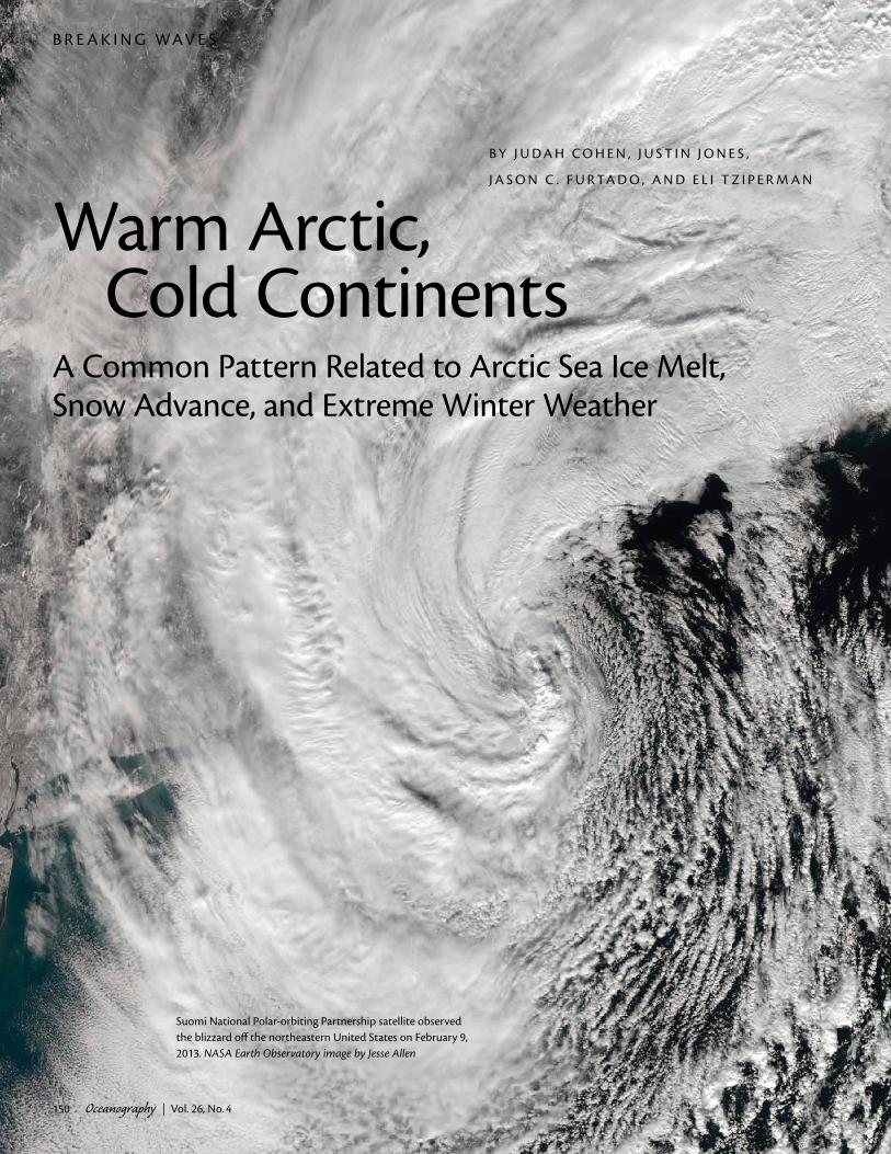
Suomi National Polar-orbiting Partnership satellite observed the blizzard off the northeastern United States on February 9, 2013. NASA Earth Observatory image by Jesse Allen

B Y J U D A H C O H E N , J U S T I N J O N E S ,

J A S O N C . F U R TA D O , A N D E L I T Z I P E R M A N

Warm Arctic, Cold ContinentsA Common Pattern Related to Arctic Sea Ice Melt, Snow Advance, and Extreme Winter Weather

Oceanography | Vol. 26, No. 4150

Oceanography | December 2013 151

the negative AO phase, Arctic weather is relatively mild, while severe winter weather increases across the Northern Hemisphere extratropical continents, including more frequent cold-air out-breaks and storminess. In contrast, during the positive AO phase, cold air masses remain locked in the Arctic, favoring persistence of a milder winter weather regime in the mid-latitudes (Thompson and Wallace, 2001). Consequently, the ability to predict the correct AO phase and amplitude would provide significant forecast skill for winter surface temperatures (Cohen and Jones, 2011). The forecast challenge is that the AO is considered unpredictable beyond a week or so and to date has not

been successfully predicted by dynamical models (Hoskins, 2013). However, recent research suggests high-latitude bound-ary conditions could force the AO phase and, hence, they could be exploited for seasonal forecasts. Specifically, low sea ice and high snow cover are related to a predominantly negative AO phase during winter (Cohen et al., 2012a; Liu et al., 2012).

Arctic sea ice plays an important role in modulating surface condi-tions at high latitudes, and even small changes in sea ice extent can cause Arctic climate to change dramatically, with ensuing feedbacks on the entire Earth climate system. During winter, sea ice decouples the ocean surface from the overlying atmosphere, prevent-ing moderation of Arctic air masses by latent and sensible heat fluxes from the Arctic Ocean. Furthermore, snow accumulation on sea ice mimics the cooling impact of snow cover over land and, hence, amplifies polar cooling dur-ing the long polar night. Anomalously low sea ice during summer exposes darker (i.e., low albedo) ocean water to sunlight, producing strong Arctic warming via direct radiative impacts and anomalous latent and sensible heat fluxes that persist into the winter months. The ensuing feedback leads to amplified warming of the Arctic relative to the rest of the globe (e.g., Serreze and Francis, 2006; Screen and Simmonds, 2010; Screen et al., 2012). Therefore, the impacts of observed (e.g., Serreze et al.,

ABSTR AC T. Arctic sea ice was observed to be at a new record minimum in September 2012. Following this summer minimum, northern Eurasia and much of North America experienced severe winter weather during the winter of 2012/2013. A statistical model that used Eurasian snow cover as its main predictor successfully forecast the observed cold winter temperatures. We propose that the large melting of Arctic sea ice may be related to the rapid advance of snow cover, similar to the connection made in studies of past climates between low Arctic sea ice and enhanced continental snowfalls and glacial inception via ice sheet growth. Regressions between autumnal sea ice extent and Eurasian snow cover extent and Northern Hemisphere temperatures yield the characteristic “warm Arctic/cold continents” pattern. This pattern was observed during winter 2012/2013, and it is common among years with observed low autumn sea ice, rapid autumn snow cover advance, and a negative winter Arctic Oscillation. Dynamical models fail to capture this pattern, instead showing maximum warming over the Arctic Ocean and widespread winter warming over the adjacent continents. We suggest that the simulated widespread warming may be due to incorrect sea ice-atmosphere coupling, including an incorrect triggering of positive feedback between low sea ice and atmospheric convection, resulting in significant model errors that are evident in seasonal predictions and that potentially impact future climate change projections.

Warm Arctic, Cold ContinentsA Common Pattern Related to Arctic Sea Ice Melt, Snow Advance, and Extreme Winter Weather

INTRODUC TIONAir-sea interaction is thought to domi-nate climate variability on seasonal to longer time scales (Goddard et al., 2012). Over the past several decades, the focus of seasonal prediction has been air-sea interaction in the tropics, specifi-cally that associated with the El Niño-Southern Oscillation (ENSO; Rasmusson and Carpenter, 1982; Alexander et al., 2002), with the assumption that knowl-edge of ENSO’s state provides most of the skill in seasonal forecasts (Hoskins, 2013). Recently, however, there has been interest in the high latitudes and the possibility that air-sea interaction in the Arctic could be forcing teleconnec-tion patterns and remotely influencing weather in the mid-latitudes (Greene and Monger, 2012).

The dominant mode of atmo-spheric climate variability in the Northern Hemisphere extratropics is the Arctic Oscillation (AO). During

Judah Cohen (jcohen@aer.com) is Director, Seasonal Forecasting, Justin Jones is Staff

Scientist, and Jason C. Furtado is Staff Scientist, all at Atmospheric and Environmental

Research, Lexington, MA, USA. Eli Tziperman is the Pamela and Vasco McCoy Jr. Professor

of Oceanography and Applied Physics, Department of Earth and Planetary Sciences and

School of Engineering and Applied Sciences, Harvard University, Cambridge, MA, USA.

Oceanography | December 2013 151

Oceanography | Vol. 26, No. 4152

2007; Stroeve et al., 2011) and projected (e.g., Holland et al., 2006; Overland et al., 2012; Stroeve et al., 2012) future changes in Arctic sea ice extent and thickness are of high priority for evaluation of model projections of future climate in a warm-ing world. Various observational and numerical studies indicate a relationship in which anomalously low (high) sea ice extent during the late boreal summer favors a negative (positive) AO the fol-lowing winter (Alexander et al., 2004; Deser et al., 2004; Magnusdottir et al., 2004; Honda et al., 2009; Hopsch et al., 2012; Jaiser et al., 2012; Liu et al., 2012).

Cohen and Entekhabi (1999) first reported moderate correlations between fall Eurasian snow cover extent and the winter AO, and subsequent modeling studies confirmed the relationship (Gong et al., 2002; Fletcher et al., 2007; Orsolini and Kvamsto, 2009; Allen and Zender, 2011). Recently, Cohen and Jones (2011) developed a new snow cover index that measures the daily rate of snow-cover change rather than its monthly mean extent. This new index is referred to as the snow advance index (SAI) and is highly correlated with the winter AO (r ~ 0.8). A proposed dynamical argu-ment for this statistical correlation is that a greater or more rapid snow cover extent leads to a strengthened and expansive Siberian high, which enhances vertical Rossby wave energy propagation from the troposphere into the strato-sphere, weakens the stratospheric polar vortex, and contributes to a negative AO at the surface (Cohen et al., 2007).

Arctic sea ice and snow cover may be related. Cohen et al. (2012a) hypoth-esized that melting Arctic sea ice could contribute to both increased fall snow cover and a negative winter AO. Still, a relationship between decreased sea

ice and increased snow cover has not been rigorously demonstrated through observational analysis, though it has been shown in modeling studies (Ghatak et al., 2010, 2012). Using a mesoscale model, Strey et al. (2010) and Porter et al. (2010) show that sea ice decline does result in warming and moistening of the Arctic boundary layer during the late summer and fall, impacting weather pat-terns locally and remotely. This warmer, moister air mass extended onto the adja-cent continents and affected snow cover across Eurasia (Strey et al., 2010).

Less sea ice leading to more snowfall is also consistent with a large body of research on glacial cycles, suggesting that less sea ice increases the availabil-ity of atmospheric moisture and favors increased snowfall, possibly playing an important role in glacial cycle dynamics (Stokes, 1955; Ewing and Donn, 1956; Le Treut and Ghil, 1983; Gildor and Tziperman, 2003).

If variations in sea ice and snow cover truly force winter weather, then knowledge of observed anomalies in each could be exploited for seasonal predictions. Eurasian snow cover extent and the SAI are currently employed in an operational statistical model whose accuracy is in great part derived from using the Eurasian October snow cover to predict the phase and amplitude of the following winter AO (Cohen and Fletcher, 2007; Cohen et al., 2010, 2012a; Cohen and Jones, 2011).

Though seasonal forecasting has traditionally relied on statistical tech-niques to predict sensible weather, more emphasis has been placed in recent years on dynamical models because they out-perform statistical models in predicting phenomena such as ENSO (Barnston et al., 2012). Indeed, fully coupled and

complex dynamical models are the dom-inant forecast tool at leading govern-ment forecast centers (National Research Council, 2010). Dynamical models have the advantage of representing many of the physical processes and couplings in the ocean-land-ice-atmosphere system. The dynamical models used for sea-sonal prediction are similar to climate models used for longer-term climate projection. Therefore, any strengths and weaknesses in dynamical models used in seasonal prediction are likely inherent in dynamical models used for climate change projections.

Below, we illustrate how sea ice and snow cover relate to variations in the AO and, hence, may be related to the large-scale atmospheric circulation pat-tern. We postulate possible dynamical errors in sea ice-atmosphere coupling rel-evant to the seasonal prediction problem and discuss how lessons from both warm and cold past climates provide valuable insights for future climate projections.

FALL 2012Arctic sea ice extent has changed dramatically over the past decade (e.g., Serreze et al., 2007; Stroeve et al., 2011). Modern-day record minima in observed sea ice extent occurred in September 2007 and again in September 2012—falling below 4 million km2 for the first time in the observational record, about half its value since 1979 (Figure 1a).

Over the past decade, fall sea ice declined and fall Eurasian snow cover increased (Cohen et al., 2012a). Eurasian snow cover extent was also above normal in October 2012. But, more impressively, the SAI, where snowfalls later in the month contribute to higher values than snowfalls earlier in the month, posted

Oceanography | December 2013 153

the second highest value observed since 1997. Figure 1b shows the date of the first snow cover in October 2012 and illustrates rapid snow cover advance later in the month.

LESS SEA ICE LEADS TO MORE SNOW COVER?Has the dramatic decline in sea ice con-tributed to the observed increased snow-fall? Sea ice decline has been particularly remarkable in the Kara, Laptev, and Chukchi Seas, which lie north of Siberia. Such a dramatic change in sea ice extent

in the region bordering the Siberian coast is likely to have a profound impact on the hydroclimatology of the region by providing a significantly larger area of open ocean, greatly increasing moisture availability and near-surface tempera-tures (Holland et al., 2007; Stroeve et al., 2007; Lawrence et al., 2008).

The large negative trend in the sea ice record makes defining the relationship between the interannual variability of sea ice and of snow cover challenging. The raw data exhibit modest negative correlations between Arctic sea ice and

continental snow cover, supporting the hypothesis that less sea ice is con-ducive to more expansive snow cover (Figure 2a). However, when the data are detrended, correlations between interan-nual sea ice and snow cover interannual anomalies are closer to zero (Figure 2b).

We make the case that the strongly correlated multidecadal trend in sea ice and snow accumulation is, perhaps, as indicative of the relevant physics as a more significant interannual correla-tion between the two. Figure 2c plots the percent difference in both sea ice

Figure 1. Dramatic sea ice melting during September 2012, rapid snow advance over Eurasia in October 2012, and further sea ice decline in the Barents Sea in November 2012. (a) Percent sea ice extent anomalies for September 2012. (b) First date that daily snow cover was observed in October 2012. (c) Percent sea ice extent anomalies for November 2012. Anomalies are derived from means of sea ice based on the full record length of 1979 to 2012. Below-normal sea ice is shown in yellows and browns. Sea ice data were downloaded from the Hadley Centre Sea Ice and Sea Surface Temperature data set (Rayner et al., 2003) and snow cover data from the Interactive Multisensor Snow and Ice Mapping System (IMS; Ramsay, 1998).

c 908070605040302010–10–20–30–40–50–60–70–80–90

Sea

Ice

Ano

mal

y (%

)

b Oct 30

Oct 25

Oct 20

Oct 15

Oct 10

Oct 5

Initi

al S

now

Cov

er D

ate

Sea

Ice

Ano

mal

y (%

)

908070605040302010–10–20–30–40–50–60–70–80–90

a

Figure 2. Statistical analysis and an atmospheric pressure pattern suggest a relationship between sea ice and Eurasian snowfall. (a) Correlation between September sea ice and October snow cover (1979–2012). (b) Same as (a) but for detrended data. In (a) and (b), blue shading shows the relationship between less sea ice and increased snow cover. (c) Composite difference in sea ice for September and for snow cover extent for October for the periods 2002–2012 minus 1991–2001, with above-normal snow cover shown in red and below-normal snow cover in blue. Contours show the correlation of October snow cover extent with October sea level pressure every 0.1 starting from 0.3 for the period 1979–2012. Positive values have solid contour lines and negative values have dashed contour lines. Snow cover data were provided by Rutgers Global Snow Lab (Robinson et al., 1993).

cba

Oct

ober

Sno

w C

over

Di�

eren

ce (%

) 45403530252015105–5–10–15–20–25–30–35–40–45

Sept

embe

r Sea

Ice

Di�

eren

ce (%

) 45403530252015105–5–10–15–20–25–30–35–40–45

Corr

elat

ion

0.70.60.50.40.30.20.1–0.1–0.2–0.3–0.4–0.5–0.6–0.7

Oceanography | Vol. 26, No. 4154

If there is a connection among reduced sea ice, greater snow-cover extent, and more severe winter weather, then the warm Arctic/cold continents pattern should be common to variability patterns of both sea ice and snow cover. Figure 3 highlights these connections in the observations. The characteristic negative AO pattern for December to February (DJF) zonal-mean tempera-ture anomalies shows warm anomalies throughout the Arctic atmosphere, peaking in the lower stratosphere, with cooling in the mid-latitude troposphere and at the surface (Figure 3a). When DJF zonal-mean temperature anomalies are regressed onto the raw (inverted) autumn Arctic sea ice extent index (Figure 3b), the resulting regression pat-tern bears similarities to the negative AO pattern, particularly in the Arctic.

and snow cover between two periods, 2002–2012, when sea ice was diminished in extent, and 1991–2001, when sea ice was more extensive. October snow cover is more extensive across the high-latitude continents in the latter period when September sea ice was low, especially in the Arctic seas that lie between Siberia and Alaska. The contours show the corre-lation coefficients between October snow cover and October sea level pressure. More extensive snow cover occurs with higher sea level pressure across northern Eurasia and adjacent Arctic waters with lower sea level pressure south of 60°N. The clockwise atmospheric flow around the area of anomalous high pressure passes directly over the region of greatest Arctic sea ice melt and is likely moistened by the newly open waters, leading to enhanced continental snowfall.

WARM ARC TIC , COLD CONTINENTSOverland et al. (2011) link the warm surface temperatures in the Arctic observed during the past few years with cold continental winters. They argue that amplified Arctic warming weakens the climatologically strong atmospheric vortex over the high latitudes, resulting in a stronger high-pressure center over the Arctic and increased meridional flow that transports cold Arctic air to lower latitudes. With greater Arctic heights and north-south transport of air masses, they find that cold air outbreaks in lower latitudes have increased in frequency. This phenomenon is referred to as the warm Arctic/cold continents pattern and is most closely associated with loss of sea ice as increasing retreat of the ice results in warming of the Arctic atmosphere.

Figure 3. Evidence that the “warm Arctic/cold continent” pattern is associated with a negative Arctic Oscillation (AO), low sea ice, and large snow cover extent. (a) Linearly detrended December to February (DJF) zonal-mean air temperature anomalies (K) regressed onto the linearly detrended and inverted standardized DJF AO index over the period 1979–2011. Contour interval every 0.2K (…–0.3, –0.1, 0.1, 0.3…). (b) As in (a) but for the inverted

and standardized September to November (SON) Arctic sea ice extent index. Trends are included in the zonal-mean temperature and Arctic sea ice extent index. (c) As in (b) but for the detrended temperature field and sea ice extent index. Contour interval every 0.1K (…–0.15, –0.05, 0.05, 0.15…). (d) As in (c) but using the detrended October Eurasian snow cover index. All atmospheric data were downloaded from the NCEP/NCAR reanalysis (Kalnay et al., 1996). (e) As in (c) but using fields from a twentieth-century CCSM4 climate reconstruc-tion run. Contour interval every 0.2K (…-0.3, -0.1, 0.1, 0.3…). The relationship among negative AO, less sea ice, and more snow cover with warm temperatures is shown in red. An ocean mask is applied to all latitudes equatorward of 70°N. Thick brown lines denote regression coefficients significant at p < 0.1 levels based on a two-tailed Student t test. Regressions onto January to March zonal mean air temperatures yielded similar results.

20°N 40°N 60°N 80°N

(a) Detrended DJF [T] Regressed onto theDetrended & Inverted DFJ AO Index

10

50

100

300500

1,000

Pres

sure

(hPa

)

20°N 40°N 60°N 80°N

(d) Detrended DJF [T] Regressed onto theDetrended October Eurasion Snow Index

10

50

100

300500

1,000

Pres

sure

(hPa

)

0.95

0.00

–0.95

K

20°N 40°N 60°N 80°N

(e) Detrended DJF [T] Regressed onto theDetrended & Inverted SON Arctic SIE Index (CCSM4)

10

50

100

300500

1,000

Pres

sure

(hPa

)

2.5

0.0

–2.5

K

2.5

0.0

–2.5

20°N 40°N 60°N 80°N

(c) Detrended DJF [T] Regressed onto theDetrended & Inverted SON Arctic SIE Index

10

50

100

300500

1,000

Pres

sure

(hPa

)

0.95

0.00

–0.95

K

20°N 40°N 60°N 80°N

(b) DJF [T] Regressed onto theInverted SON Arctic SIE Index

10

50

100

300500

1,000

Pres

sure

(hPa

)

2.5

0.0

–2.5

KK

Oceanography | December 2013 155

However, upon detrending the tempera-ture and sea ice extent index, the regres-sion pattern changes considerably, and instead the familiar warm Arctic/cold continents pattern emerges (Figure 3c; Overland et al., 2011). Similarly, regres-sion of DJF zonal-mean temperature anomalies onto the detrended October Eurasian snow cover index (Robinson et al., 1993) also shows the warm Arctic/cold continents pattern (Figure 3d).

Further analysis performed with zonal-mean zonal wind anomalies shows that a negative winter AO, increased Eurasian October snow cover, and decreased sea ice extent are all associ-ated with a shift in the high-latitude jet stream, with weakening of the polar jet and strengthening of the subtropical jet (Figure 4). The results were found to be significant for the AO, snow cover, and raw sea ice, but not for detrended sea

ice. The relationship between sea ice and the jet stream shift is consistent with the research of Francis and Vavrus (2012).

WINTER 2013 FORECASTSFigure 5 shows observed and predicted January to March 2013 surface tempera-ture anomalies. The statistical model, based on the SAI of 2σ, correctly predicts both a strongly negative winter AO (less than –1.5σ) and cold temperatures across northern Eurasia and most of the United States. The hemispheric pattern correla-tion between predicted and observed temperatures is 0.65, and the root mean square error is 0.87°C. Both skill metrics are extremely high for seasonal forecasts. Given the published skill of the model from hindcasts (Cohen and Fletcher, 2007; Cohen and Jones, 2011), past suc-cesses of operational forecasts (Cohen et al., 2010, 2012a), and the success of

the winter 2013 forecast, it is highly probable that this winter’s severe weather was related to the rapid advance in snow cover in the fall. Though no known empirical forecast model directly incor-porates sea ice extent for winter seasonal forecasts, the severe winter weather is also consistent with the extremely low sea ice observed in fall 2012.

As discussed above, the pattern that may best relate low sea ice, extensive snow cover, and negative AO is the warm Arctic/cold continents temperature pat-tern in winter. Figure 6b plots daily stan-dardized polar cap geopotential height (PCH; i.e., geopotential height anomalies area-averaged poleward of 60°N) anoma-lies from October 2012 through March 2013 from the surface to 10 hPa; these geopotential height anomalies are also a good proxy for temperature anomalies (positive height values indicate warmer

(a) Detrended DJF [U] Regressed onto theDetrended & Inverted DFJ AO Index

20°N 40°N 60°N 80°N

m s–1

5.5

0.0

–5.5

10

50

100

300500

1,000

Pres

sure

(hPa

)

(c) Detrended DJF [U] Regressed onto theDetrended & Inverted SON Arctic SIE Index

20°N 40°N 60°N 80°N

m s–1

1.5

0.0

–1.5

10

50

100

300500

1,000

Pres

sure

(hPa

)

(b) DJF [U] Regressed onto theInverted SON Arctic SIE Index

20°N 40°N 60°N 80°N

m s–1

5.5

0.0

–5.5

10

50

100

300500

1,000

Pres

sure

(hPa

)

(d) Detrended DJF [U] Regressed onto theDetrended October Eurasion Snow Index

20°N 40°N 60°N 80°N

m s–1

1.5

0.0

–1.5

10

50

100

300500

1,000

Pres

sure

(hPa

)

(e) Detrended DJF [U] Regressed onto theDetrended & Inverted SON Arctic SIE Index (CCSM4)

20°N 40°N 60°N 80°N

1.5

0.0

–1.5

m s–1

10

50

100

300500

1,000

Pres

sure

(hPa

)

Figure 4. Evidence that a negative Arctic Oscillation, low sea ice, and large snow cover extent are all associated with weakening of the polar jet and strengthen-ing of the subtropical jet. (a) Linearly detrended December to February (DJF) zonal-mean zonal wind anomalies (m s–1) regressed onto the linearly detrended and inverted standardized DJF AO index over the period 1979–2011. Contour interval every 0.5 m s–1. (b) As in (a) but for the

inverted and standardized September to November (SON) Arctic sea ice extent index. Trends are included in the zonal-mean zonal wind and Arctic sea ice extent index. (c) As in (b) but for the detrended zonal wind field and sea ice extent index. Contour interval every 0.25 m s–1. (d) As in (c) but for using the detrended October Eurasian snow cover index. All atmospheric data downloaded from the NCEP/NCAR reanalysis (Kalnay et al., 1996). (e) As in (c) but fields from a twentieth-century CCSM4 climate reconstruction run. Thick brown lines denote regression coefficients significant at the p < 0.1 levels based on a two-tailed Student t test.

Oceanography | Vol. 26, No. 4156

of international models, can be found at http://www.cpc.ncep.noaa.gov/products/NMME). The dynamical model fore-casts are similar to each other and can be characterized by pervasive warmth at high latitudes that extends across much of the Northern Hemisphere continents, including all of northern Eurasia and the United States (Figure 7a). The most notable feature is a bull’s-eye of above-normal temperatures predicted by the suites of models in the Barents Sea north of Norway and Russia in the Arctic Ocean. This local maximum coincides with a region of maximum sea ice loss in November 2012 (Figure 1c), which was used to initialize the dynamical models. Compared with the observed temperature anomalies (Figure 5a), the dynamical model forecasts were poor, incorrectly predicting warm tempera-tures across the northern continents for January to March 2013.

The fact that the forecasted region of maximum positive temperature anomalies in the dynamical models and the large region of anomalously low or missing sea ice are co-located is unlikely to be a coincidence. Leibowicz et al. (2012) show that late fall and winter dynamical model variability in the Arctic involves coupling between negative sea ice anomalies and deep atmospheric convection and convective precipitation, especially in the Barents Sea, due to trig-gering of the convective cloud feedback. This feedback has also been shown to be important in explaining equable (warm) climates in the geological past (Abbot and Tziperman, 2008, 2009). The precipi-tation forecast from the same ensemble mean of American models shows above-normal precipitation predicted in the same Barents Sea region (not shown), supporting the possibility of atmospheric

temperatures in the Arctic). We also regressed sea ice extent anomalies with polar cap heights for the same period (Figure 6a). High geopotential heights in the troposphere, especially during fall and mid to late winter, dominate the plot. Similar regressions with October snow cover and the AO also show pre-dominately high geopotential heights in the troposphere throughout the period (not shown). In contrast, in the stratosphere, negative PCH anomalies prevailed through December, abruptly becoming positive for most of January (due to a major sudden stratospheric warming) and then returning to below average conditions in March. Regression of sea ice and snow cover with the PCHs also shows warming in the strato-sphere in January.

Figure 6 also includes some of the extreme weather events observed with each warming pulse of the polar cap. This figure suggests that there may be a link between decreased sea ice, exten-sive snow cover, the negative AO, and extreme/severe winter weather. When

the Arctic is warm and dominated by high pressure, the jet stream weakens and shifts equatorward, and atmospheric blocking is more prevalent (Rex, 1950). As a result, temperatures turn colder over the continents, and snowstorms are more likely in the population centers of the United States, Europe, and East Asia. During the six months between October 2012 and March 2013, the troposphere in the Arctic was overwhelmingly dominated by above-normal geopotential height and warm temperatures, consis-tent with a favored or increased prob-ability of extreme weather events (Cohen et al., 2010), starting with Superstorm Sandy (Greene et al., 2013) and ending with record cold and snow in March 2013 across both the United States and Europe.

DYNAMICAL FORECASTS FOR WINTER 2013Figure 7 shows the January through March 2013 real-time surface tem-perature forecast for an ensemble of American numerical models (individual model forecasts, including an ensemble

Figure 5. Winter temperature forecast based on the Snow Advance Index shows remarkable agreement with observations. Observed and forecast surface temperature anomalies in °C for January to March 2013 for the Northern Hemisphere. Forecast was issued in early December. Normal defined as average tem-perature from 1981 to 2010. Below-normal temperatures are shaded in blue.

2.51.51.00.80.60.40.20.1–0.1–0.2–0.4–0.6–0.8–1.0–1.5–2.5

°C

(a) Observed Temperature AnomalyJan–Mar 2013

(b) AER Forecast Temperature AnomalyJan–Mar 2013

Oceanography | December 2013 157

convection there. The tendency of the convective cloud feedback to trigger abruptly beyond some threshold forc-ing (Abbot and Tziperman, 2008, 2009) implies that some seasonal prediction models may trigger it prematurely or fail to trigger it when needed. Then, long-wave cloud radiative forcing due to cloud cover during the polar night can amplify and spread heating in regions of sea ice retreat in the models.

If sea ice, atmospheric pressure, and cryosphere-climate coupling in general are indeed an important part of the dynamics behind the predictability skill demonstrated by the SAI, such incor-rect triggering could explain some of the failure of dynamical models to achieve comparable prediction skill. Specifically, this could explain the incorrect large-scale temperature pattern of warming centered on the region of greatest sea ice loss and perhaps even the lack of continental cooling. However, we can-not rule out that other factors, such as boundary-layer stratification, surface turbulent fluxes, cloud-radiation interac-tions, and ocean stratification may have been as or more important in producing the poor model forecasts.

As an initial test of whether the simu-lated link between autumn Arctic sea ice extent and wintertime hemispheric temperatures is correct, we regress the zonal-mean temperature anomalies onto the detrended sea ice extent index from the historical run (i.e., a reconstruction of twentieth century climate; Taylor et al., 2012) of the Community Climate System Model version 4 (CCSM4; Gent et al., 2011). Figure 3e shows that the warm Arctic/cold continent response to sea-ice anomalies is not seen in CCSM4 and suggests that the temperature relations to Arctic sea ice loss across the Northern

Hemisphere continents are out of phase with the observed results (Figure 3c). This divergence in the temperature struc-ture is also consistent with that between the forecasts from the dynamical models and the observed temperatures for winter 2013 (Figures 5a and 7a). The dynamical model does seem to do a better job of simulating the weakening of the polar jet and strengthening of the subtropical jet, as observed when Arctic sea ice is low.

Correct cryosphere-climate coupling

is critical for simulating and, therefore, predicting winter climate not only on a seasonal scale but also on longer scales. Cohen et al. (2012a) argue that poor simulation of Eurasian fall snow cover trends in dynamical models has led to incorrect temperature trends across the extratropical Northern Hemisphere in winter, where winter warming is simulated instead of the observed win-ter cooling over the past two to three decades. It has also been demonstrated

Major Strato-spheric

Warming

Late Season Snow/ Arctic

Outbreaks US & Europe

Midwest-East Coast

Snowstorm

Blizzard New

England

Blizzard 2013

Snow in theUK/Arctic

Outbreak US

Blizzards in the US

Cold/Snow Asia, Europe

Early Nor’easter

Sandy

(b) Winter 2012–2013 Polar Cap Height 60°–90°N

(a) Winter 2012–2013 Polar Cap Height 60°–90°N (Contribution From Sea Ice)

10

50

100

300500

1,000

Pres

sure

(hPa

)

10

50

100

300500

1,000

Pres

sure

(hPa

)

01O

ct

15O

ct

01N

ov

15N

ov

01D

ec

15D

ec

01Ja

n

15Ja

n

01Fe

b

15Fe

b

01M

ar

15M

ar

2.01.61.20.80.40.0–0.4–0.8–1.2–1.6–2.0

Stan

dard

ized

Ano

mal

ies

1.00.80.60.40.20.0–0.2–0.4–0.6–0.8–1.0

Stan

dard

ized

Ano

mal

ies

Figure 6. Indications of a link among decreased sea ice, extensive snow cover, negative AO, and extreme/severe winter weather, possibly via stratospheric warming in January. (a) Regression of September 2012 sea ice extent anomalies onto daily standardized polar cap geopotential height from 10–1,000 hPa defined as the areal average of the standardized geopotential height anomalies poleward of 60°N from October 1, 2012, through March 31, 2013. (b) Anomalies of daily standardized polar cap geopotential height from October 1, 2012, through March 31, 2013. High geopotential heights/warm temperatures are shaded in red. Blue arrows denote severe winter weather events across the Northern Hemisphere, and the red arrow shows the date of a sudden major stratospheric warming.

Oceanography | Vol. 26, No. 4158

that dynamical models poorly simulate the atmospheric response to snow cover (Hardiman et al., 2008; recent work of authors Furtado and Cohen and col-leagues). Could systemic errors in cryo-sphere-climate coupling also jeopardize future projections of winter temperatures due to anthropogenic global warming?

Figure 7b plots projected temperature anomalies relative to current climatol-ogy for Northern Hemisphere winter from a suite of CMIP5 (Coupled Model Intercomparison Project phase-5) models. The projection shows warm-ing everywhere across the Northern Hemisphere, but the greatest warming is located over the Arctic Ocean, with a maximum over the Barents Sea. The warming pattern is reminiscent of the incorrect seasonal temperature forecasts for winter 2013. It is also similar to the convective cloud feedback in reanalysis models (Leibowicz et al., 2012) and some

Intergovernmental Panel on Climate Change (IPCC) models (Abbot et al., 2009). It is not possible to tell whether the triggering of this feedback in the context of a global warming prediction is correct or not, yet it presents an added uncertainty in future climate projections.

CONCLUSIONSThe winter of 2012/2013 continued a string of severe winters across the Northern Hemisphere continents. While coupled models predict that warming due to anthropogenic forcing would be greatest in the boreal winter season, over the past two to three decades, the warm-ing trend has been muted in the winter season over some Northern Hemisphere land areas, while warming has continued in the other three seasons (Cohen et al., 2012b). Cohen et al. (2012a) proposed that sea ice loss has contributed to moist-ening of the Arctic, which has resulted

in more extensive snow cover in the fall that in turn forced a dynamical response in the atmosphere favorable to a negative winter AO. The enhanced snow accumu-lation is also consistent with the idea that low sea ice and warm temperatures lead to enhanced snow accumulation and ice age inception (Stokes, 1955; Ewing and Donn, 1956; Le Treut and Ghil, 1983; Gildor and Tziperman, 2003).

September 2012 sea ice melt achieved a new record in the satellite era, fol-lowed by a near-record rapid advance in snow cover in October. A statistical model using snow cover as its main predictor accurately forecasted below-normal temperatures across northern Eurasia and the United States during winter 2013. Furthermore, the large melt of Arctic sea ice in summer/fall 2012, the rapid advance of snow cover across Eurasia in October 2012, and the pre-dominantly negative AO phase during winter 2012/2013 may all be associated with severe winter weather across the northern continents. The PCHs show that high geopotential heights and a warm Arctic dominated the period of October 2012 to March 2013 (Figure 6), with episodic pulsing or strengthen-ing of the positive PCH anomalies (or, equivalently, temperature anomalies). Figures 3 and 6 show that low sea ice, extensive snow cover, and a negative winter AO share the warm Arctic/cold continents pattern and are linked with increased atmospheric blocking and extreme winter weather across the Northern Hemisphere.

Dynamical models produced uni-versally poor temperature forecasts for winter 2013. We hypothesize that the erroneous predicted model warmth across the northern continents and sea ice retreat may be related. Furthermore,

Figure 7. Dynamical model predictions of winter 2012 temperatures diverged from observations. They show a strong bull’s-eye of warming over the Barents Sea in the Arctic that is not seen in observations. The pattern of warming is reminiscent of coupled model future temperature projections. (a) Surface air temperature anomalies in °C. National Multi-Model Ensemble (NMME) models used to compute the ensemble-mean include CFSv1, CFSv2, GFDL-CM2.2, IRI-ECHAM4-f, IRI-ECHAM4-a, CCSM3.0, and GEOS5. Data were downloaded from http://www.cpc.ncep.noaa.gov/products/NMME/. (b) Composite differences in surface air temperature (K) between 2079 and 2100, minus 1979 to 2000. The future sce-nario used is the rcp45 (a moderate emissions scenario; i.e., the radiative forcing reaches 4.5 Wm–2 by 2100). Models predict the greatest warming will be in the region of largest Arctic sea ice loss. Coupled Model Intercomparison Project phase-5 (CMIP5) models used to compute the ensemble-mean include BCC-CSM1-1, CCSM4, CNRM-CM5, CSIRO-Mk3-6-0, GFDL-CM3, GISS-E2-H, GISS-E2-R, INMCM4, MIROC5, MIROC-ESM, MPI-ESM-LR, MRI-CGCM3, NorESM1-M, and NorESM1-ME.

°C

7.006.005.004.003.002.001.000.500.25–0.25–0.50–1.00–2.00–3.00–4.00–5.00–6.00–7.00

a b

Oceanography | December 2013 159

the maximum in temperature anoma-lies over the Barents Sea, which extends deep into the continental interior in the dynamical model seasonal forecasts, may offer a cautionary tale regarding a similar pattern in climate change projec-tions. The strong coupling between sea ice and atmosphere, possibly via convec-tive feedback in the dynamical models, may disrupt the coupling between a warm Arctic and cold continents found in observations. These lessons from seasonal prediction indicate that rapid response of sea ice to external forcing, as expressed in past abrupt climate change (Gildor and Tziperman, 2003), may lead to future surprises in the Arctic, thus increasing the uncertainties in future climate projections for the entire Northern Hemisphere.

ACKNOWLEDGEMENTSJ.C. is supported by National Science Foundation grant BCS-1060323 and National Oceanic and Atmospheric Administration grant NA10OAR- 4310163. E.T. was supported by grant DE-SC0004984 from the Department of Energy Climate and Environmental Sciences Division, Office of Biological and Environmental Research, and he thanks the Weizmann Institute for hospi-tality received during parts of this work. We also thank the climate modeling groups working as part of CMIP5 for producing and making available their model output for analysis. We thank two anonymous reviewers for constructive comments that led to improvement of the manuscript.

REFERENCESAbbot, D.S., and E. Tziperman. 2008. Sea ice, high

latitude convection, and equable climates. Geophysical Research Letters 35, L03702, http://dx.doi.org/10.1029/2007GL032286.

Abbot, D.S., and E. Tziperman. 2009. Controls on the activation and strength of a high latitude convective-cloud feedback. Journal of Atmospheric Sciences 66:519–529, http://dx.doi.org/10.1175/2008JAS2840.1.

Abbot, D.S., C. Walker, and E. Tziperman. 2009. Can a convective cloud feedback help to elimi-nate winter sea ice at high CO2 concentrations? Journal of Climate 22(21):5,719–5,731, http://dx.doi.org/10.1175/2009JCLI2854.1.

Alexander, M.A., U.M. Bhatt, J.E. Walsh, M.S. Timlin, J.S. Miller, and J.D. Scott. 2004. The atmospheric response to realistic Arctic sea ice anomalies in an AGCM during winter. Journal of Climate 17:890–905, http://dx.doi.org/ 10.1175/1520-0442(2004)017<0890:TARTRA> 2.0.CO;2.

Alexander, M.A., I. Blade, M. Newman, J.R. Lanzante, N.-C. Lau, and J.D. Scott. 2002. The atmospheric bridge: The influ-ence of ENSO teleconnections on air-sea interaction over the global oceans. Journal of Climate 15:2,205–2,231, http://dx.doi.org/ 10.1175/1520-0442(2002)015<2205:TABTIO>2.0.CO;2.

Allen, R.J., and C.S. Zender. 2011. Forcing of the Arctic Oscillation by Eurasian snow cover. Journal of Climate 24:6,528–6,539, http://dx.doi.org/10.1175/2011JCLI4157.1.

Barnston, A.G., M.K. Tippett, M.L. L’Hereux, S. Li, and D.G. DeWitt. 2012. Skill of real-time sea-sonal ENSO model predictions during 2002–11. Bulletin of the American Meteorological Society 93:631–651, http://dx.doi.org/10.1175/BAMS-D-11-00111.1.

Cohen, J., M. Barlow, P. Kushner, and K. Saito. 2007. Stratosphere-troposphere coupling and links with Eurasian land-surface variability. Journal of Climate 20:5,335–5,343, http://dx.doi.org/10.1175/2007JCLI1725.1.

Cohen, J., and D. Entekhabi. 1999. Eurasian snow cover variability and Northern Hemisphere climate predictability. Geophysical Research Letters 26:345–348, http://dx.doi.org/ 10.1029/1998GL900321.

Cohen, J., and C. Fletcher. 2007. Improved skill for Northern Hemisphere winter surface tempera-ture predictions based on land-atmosphere fall anomalies. Journal of Climate 20:4,118–4,132, http://dx.doi.org/10.1175/JCLI4241.1.

Cohen, J., J. Foster, M. Barlow, K. Saito, and J. Jones. 2010. Winter 2009/10: A case study of an extreme Arctic Oscillation event. Geophysical Research Letters 37, L17707, http://dx.doi.org/ 10.1029/2010GL044256.

Cohen, J., J.C. Furtado, M. Barlow, V. Alexeev, and J. Cherry. 2012a. Increasing fall snow cover and widespread boreal win-ter cooling. Environmental Research Letters 7, 014007, http://dx.doi.org/ 10.1088/1748-9326/7/1/014007.

Cohen, J., J.C. Furtado, M. Barlow, V. Alexeev, and J. Cherry. 2012b. Asymmetric seasonal temperature trends. Geophysical Research Letters 39, L04705, http://dx.doi.org/ 10.1029/2011GL050582.

Cohen, J., and J. Jones. 2011. A new index for more accurate winter predictions. Geophysical Research Letters 38, L21701, http://dx.doi.org/ 10.1029/2011GL049626.

Deser, C., G. Magnusdottir, R. Saravanan, and A. Phillips. 2004. The effects of North Atlantic SST and sea-ice anomalies on the winter circulation in CCM3. Part II. Direct and indirect components of the response. Journal of Climate 17:877–889, http://dx.doi.org/ 10.1175/1520-0442(2004)017<0877:TEONAS> 2.0.CO;2.

Ewing, M., and W.L. Donn. 1956. A theory of ice ages. Science 123:1,061–1,066.

Fletcher, C., P. Kushner, and J. Cohen. 2007. Stratospheric control of the extratropical circu-lation response to surface forcing. Geophysical Research Letters 34, L21802, http://dx.doi.org/ 10.1029/2007GL031626.

Francis, J.A., and S.J. Vavrus. 2012. Evidence linking Arctic amplification to extreme weather in mid-latitudes. Geophysical Research Letters 39, L06801, http://dx.doi.org/ 10.1029/2012GL051000.

Gent, P.R., G. Danabasoglu, L.J. Donner, M.M. Holland, E.C. Hunke, S.R. Jayne, D.M. Lawrence, R.B. Neale, P.J. Rasch, M. Vertenstein, and others. 2011. The Community Climate System Model version 4. Journal of Climate 24:4,973–4,991, http://dx.doi.org/10.1175/2011JCLI4083.1.

Ghatak, D., C. Deser, A. Frei, G. Gong, A. Phillips, D.A. Robinson, and J. Stroeve. 2012. Simulated Siberian snow cover response to observed Arctic sea ice loss, 1979–2008. Journal of Geophysical Research 117, D23108, http://dx.doi.org/10.1029/2012JD018047.

Ghatak, D., A. Frei, G. Gong, J. Stroeve, and D. Robinson. 2010. On the emergence of an Arctic amplification signal in terrestrial Arctic snow extent. Journal of Geophysical Research 115, D24105, http://dx.doi.org/ 10.1029/2010JD014007.

Gildor, H., and E. Tziperman. 2003. Sea-ice switches and abrupt climate change. Philosophical Transactions of the Royal Society of London A 361(1810):1,935–1,942, http://dx.doi.org/10.1098/rsta.2003.1244.

Goddard, L., J.W. Hurrell, B.P. Kirtman, J. Murphy, T. Stockdale, and C. Vera. 2012. Two time scales for the price of one (almost). Bulletin of the American Meteorological Society 93:621–629, http://dx.doi.org/10.1175/BAMS-D-11-00220.1.

Gong, G., D. Entekhabi, and J. Cohen. 2002. A large-ensemble model study of the wintertime AO/NAO and the role of inter-annual snow perturbations. Journal of Climate 15:3,488–3,499, http://dx.doi.org/ 10.1175/1520-0442(2002)015<3488:ALEMSO> 2.0.CO;2.

Greene, C.H., J.A. Francis, and B.C. Monger. 2013. Superstorm Sandy: A series of unfortu-nate events? Oceanography 26(1):8–9, http://dx.doi.org/10.5670/oceanog.2013.11.

Oceanography | Vol. 26, No. 4160

Greene, C.H., and B.C. Monger. 2012. An Arctic wild card in the weather. Oceanography 25(2):7–9, http://dx.doi.org/ 10.5670/oceanog.2012.58.

Hardiman, S.C., P.J. Kushner, and J. Cohen. 2008. Investigating the ability of general circulation models to capture the effects of Eurasian snow cover on winter climate. Journal of Geophysical Research 113, D21123, http://dx.doi.org/ 10.1029/2008JD010623.

Holland, M.M., C.M. Bitz, E.C. Hunke, W.H. Lipscomb, and J.L. Schramm. 2006. Influence of the sea ice thickness distribu-tion on polar climate in CCSM3. Journal of Climate 19:2,398–2,414, http://dx.doi.org/ 10.1175/JCLI3751.1.

Holland, M.M., J. Finnis, A.P. Barrett, and M.C. Serreze. 2007. Projected changes in Arctic Ocean freshwater budgets. Journal of Geophysical Research 112, G04S55, http://dx.doi.org/10.1029/2006JG000354.

Honda, M., J. Inue, and S. Yamane. 2009. Influence of low Arctic sea-ice minima on anomalously cold Eurasian winters. Geophysical Research Letters 36, L08707, http://dx.doi.org/ 10.1029/2008GL037079.

Hopsch, S., J. Cohen, and K. Dethloff. 2012. Analysis of a link between fall Arctic sea ice concentration and atmospheric patterns in the following winter. Tellus A 64, 18624, http://dx.doi.org/10.3402/tellusa.v64i0.18624.

Hoskins, B. 2013. The potential for skill across the range of the seamless weather-climate pre-diction problem: A stimulus for our science. Quarterly Journal of the Royal Meteorological Society 139:573–584, http://dx.doi.org/10.1002/qj.1991.

Jaiser, R., K. Dethloff, D. Handorf, A. Rinke, and J. Cohen. 2012. Impact of sea ice cover changes on the Northern Hemisphere atmospheric winter circulation. Tellus 64, 11595, http://dx.doi.org/10.3402/tellusa.v64i0.11595.

Kalnay, E., M. Kanamitsu, R. Kistler, W. Collins, D. Deaven, L. Gandin, M. Iredell, S. Saha, G. White, J. Woollen, and others. 1996. The NCEP/NCAR 40-year reanalysis proj-ect. Bulletin of the American Meteorological Society 77:437–471, http://dx.doi.org/10.1175/ 1520-0477(1996)077<0437:TNYRP>2.0.CO;2.

Lawrence, D.M., A.G. Slater, R.A. Tomas, M.M. Holland, and C. Deser. 2008. Accelerated Arctic land warming and permafrost degra-dation during rapid sea ice loss. Geophysical Research Letters 35, L11506, http://dx.doi.org/ 10.1029/2008GL033985.

Le Treut, H., and M. Ghil. 1983. Orbital forcing, climatic interactions, and glaciation cycles. Journal of Geophysical Research 88:5,167–5,190, http://dx.doi.org/10.1029/JC088iC09p05167.

Leibowicz, B.D., D.S. Abbot, K.A. Emanuel, and E. Tziperman. 2012. Correlation between present-day model simulation of Arctic cloud radiative forcing and sea ice consis-tent with positive winter convective cloud

feedback. Journal of Advances in Modeling Earth Systems 4, M07002, http://dx.doi.org/ 10.1029/2012MS000153.

Liu, J., J.A. Curry, H. Wang, M. Song, and R. Horton. 2012. Impact of declining Arctic sea ice on winter snow. Proceedings of the National Academy of Sciences of the United States of America 109:4,074–4,079, http://dx.doi.org/ 10.1073/pnas.1114910109.

Magnusdottir, G., C. Deser, and R. Saravanan. 2004. The effects of North Atlantic SST and sea-ice anomalies on the winter circulation in CCM3. Part I: Main features and storm track characteristics of the response. Journal of Climate 17:857–876, http://dx.doi.org/10.1175/ 1520-0442(2004)017<0857:TEONAS>2.0.CO;2.

National Research Council. 2010. Building blocks of intraseasonal to interannual forecasting. Pp. 54–100 in Assessment of Intraseasonal to Interannual Climate Prediction and Predictability. The National Academies Press, Washington, DC.

Orsolini, Y.J., and N.G. Kvamsto. 2009. Role of Eurasian snow cover in wintertime circula-tion: Decadal simulations forced with satel-lite observations. Journal of Geophysical Research 114, D19108, http://dx.doi.org/ 10.1029/2009JD012253.

Overland, J.E., J.A. Francis, E. Hanna, and M. Wang. 2012. The recent shift in early sum-mer Arctic atmospheric circulation. Geophysical Research Letters 39, L19804, http://dx.doi.org/ 10.1029/2012GL053268.

Overland, J.E., K.R. Wood, and M. Wang. 2011. Warm Arctic—cold continents: Climate impacts of the newly open Arctic Sea. Polar Research 30, 15787, http://dx.doi.org/10.3402/polar.v30i0.15787.

Porter, D.F., J.J. Cassano, and M.C. Serreze. 2010. Local and large-scale atmospheric responses to reduced Arctic sea ice and ocean warm-ing in the WRF model. Journal of Geophysical Research 117, D11115, http://dx.doi.org/ 10.1029/2011JD016969.

Ramsay, B.H. 1998. The interactive multisensory snow and ice mapping system. Hydrological Processes 12:1,537–1,546.

Rasmusson, E.M., and T.H. Carpenter. 1982. Variations in tropical sea surface tempera-ture and surface wind fields associated with the Southern Oscillation/El Niño. Monthly Weather Review 110:354–384, http://dx.doi.org/ 10.1175/1520-0493(1982)110<0354:VITSST>2.0.CO;2.

Rayner, N.A., D.E. Parker, E.B. Horton, C.K. Folland, L.V. Alexander, D.P. Rowell, E.C. Kent, and A. Kaplan. 2003. Global analyses of sea surface temperature, sea ice, and night marine air temperature since the late nineteenth century. Journal of Geophysical Research 108, 4407, http://dx.doi.org/10.1029/2002JD002670.

Rex, D.F. 1950. Blocking action in the middle tro-posphere and its effect upon regional climate. Tellus 2:196–211, http://dx.doi.org/ 10.1111/j.2153-3490.1950.tb00331.x.

Robinson, D.A., K.F. Dewey, and R.R. Heim Jr. 1993. Global snow cover monitoring: An update. Bulletin of the American Meteorological Society 74:1,689–1,696, http://dx.doi.org/ 10.1175/1520-0477(1993)074<1689:GSCMAU> 2.0.CO;2.

Screen, J.A., C. Deser, and I. Simmonds. 2012. Local and remote controls on observed Arctic warming. Geophysical Research Letters 39, L10709, http://dx.doi.org/ 10.1029/2012GL051598.

Screen, J.A., and I. Simmonds. 2010. The central role of diminishing sea ice in recent Arctic tem-perature amplification. Nature 464:1,334–1,337, http://dx.doi.org/10.1038/nature09051.

Serreze, M.C., and J.A. Francis. 2006. The Arctic amplification debate. Climatic Change 76(3–4):241–264, http://dx.doi.org/ 10.1007/s10584-005-9017-y.

Serreze, M.C., M.M. Holland, and J. Stroeve. 2007. Perspectives on the Arctic’s shrinking sea-ice cover. Science 315:1,533–1,536, http://dx.doi.org/10.1126/science.1139426.

Stokes, W.L. 1955. Another look at the ice age. Science 122:815–821, http://dx.doi.org/10.1126/science.122.3174.815.

Strey, S.T., W.L. Chapman, and J.E. Walsh. 2010. The 2007 sea ice minimum: Impacts on the Northern Hemisphere atmosphere in late autumn and early winter. Journal of Geophysical Research 115, D23103, http://dx.doi.org/ 10.1029/2009JD013294.

Stroeve, J., M.M. Holland, W. Meier, T. Scambos, and M. Serreze. 2007. Arctic sea ice decline: Faster than forecast. Geophysical Research Letters 34, L09501, http://dx.doi.org/ 10.1029/2007GL029703.

Stroeve, J.C., V. Kattsov, A. Barrett, M. Serreze, T. Pavlova, M. Holland, and W.N. Meier. 2012. Trends in Arctic sea ice extent from CMIP5, CMIP3 and observations. Geophysical Research Letters 39, L16502, http://dx.doi.org/ 10.1029/2012GL052676.

Stroeve, J.C., J.S. Maslanik, M.C. Serreze, I. Rigor, W. Meier, and C. Fowler. 2011. Sea ice response to an extreme negative phase of the Arctic Oscillation during winter 2009/2010. Geophysical Research Letters 38, L02502, http://dx.doi.org/10.1029/2010GL045662.

Taylor, K.E., R.J. Stouffer, and G.A. Meehl. 2012. An overview of CMIP5 and the experiment design. Bulletin of the American Meteorological Society 93:485–498.

Thompson, D.W.J., and J.M. Wallace. 2001. Regional climate impacts of the Northern Hemisphere annular mode. Science 293:85–89, http://dx.doi.org/10.1126/science.1058958.