October 23, 2003 1

Algorithms and Data StructuresLecture X

Simonas ŠaltenisAalborg Universitysimas@cs.auc.dk

October 23, 2003 2

This Lecture

Dynamic programming Fibonacci numbers example Optimization problems Matrix multiplication optimization Principles of dynamic programming Longest Common Subsequence

October 23, 2003 3

Algorithm design techniques

Algorithm design techniques so far: Iterative (brute-force) algorithms

For example, insertion sort Algorithms that use other ADTs

(implemented using efficient data structures)

For example, heap sort Divide-and-conquer algorithms

Binary search, merge sort, quick sort

October 23, 2003 4

Divide and Conquer

Divide and conquer method for algorithm design: Divide: If the input size is too large to deal

with in a straightforward manner, divide the problem into two or more disjoint subproblems

Conquer: Use divide and conquer recursively to solve the subproblems

Combine: Take the solutions to the subproblems and “merge” these solutions into a solution for the original problem

October 23, 2003 5

Divide and Conquer (2)

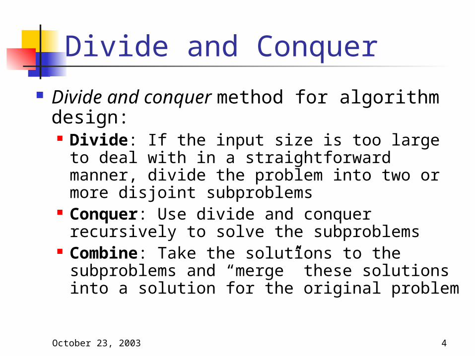
For example, MergeSort

The subproblems are independent and non-overlaping

Merge-Sort(A, p, r) if p < r then q(p+r)/2 Merge-Sort(A, p, q) Merge-Sort(A, q+1, r) Merge(A, p, q, r)

Merge-Sort(A, p, r) if p < r then q(p+r)/2 Merge-Sort(A, p, q) Merge-Sort(A, q+1, r) Merge(A, p, q, r)

October 23, 2003 6

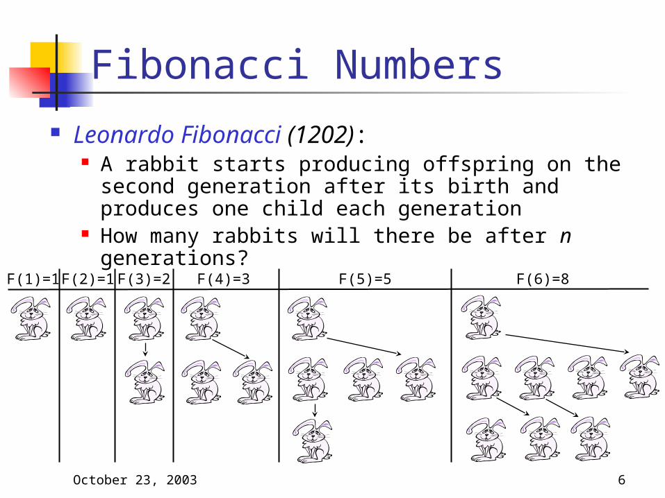
Fibonacci Numbers Leonardo Fibonacci (1202):

A rabbit starts producing offspring on the second generation after its birth and produces one child each generation

How many rabbits will there be after n generations?

F(1)=1 F(2)=1 F(3)=2 F(4)=3 F(5)=5 F(6)=8

October 23, 2003 7

Fibonacci Numbers (2)

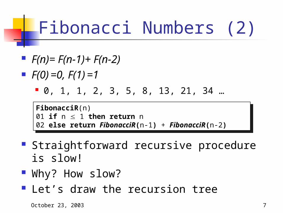
F(n)= F(n-1)+ F(n-2) F(0) =0, F(1) =1

0, 1, 1, 2, 3, 5, 8, 13, 21, 34 …

Straightforward recursive procedure is slow!

Why? How slow? Let’s draw the recursion tree

FibonacciR(n)01 if n 1 then return n02 else return FibonacciR(n-1) + FibonacciR(n-2)

FibonacciR(n)01 if n 1 then return n02 else return FibonacciR(n-1) + FibonacciR(n-2)

October 23, 2003 8

Fibonacci Numbers (3)

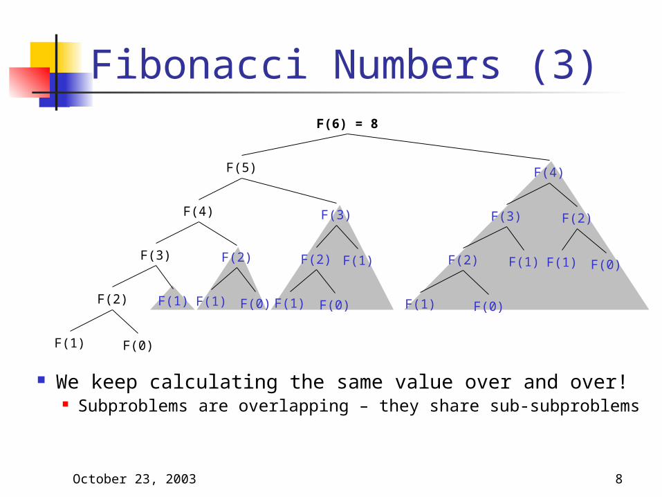
We keep calculating the same value over and over! Subproblems are overlapping – they share sub-subproblems

F(6) = 8

F(5)

F(4)

F(3)

F(1)

F(2)

F(0)

F(1) F(1)

F(2)

F(0)

F(3)

F(1)

F(2)

F(0)

F(1)

F(4)

F(3)

F(1)

F(2)

F(0)

F(1) F(1)

F(2)

F(0)

October 23, 2003 9

Fibonacci Numbers (4)

How many summations are there S(n)? S(n) = S(n – 1) + S(n – 2) + 1 S(n) 2S(n – 2) +1 and S(1) = S(0) =

0 Solving the recurrence we get S(n) 2n/2 – 1 1.4n

Running time is exponential!

October 23, 2003 10

Fibonacci Numbers (5)

We can calculate F(n) in linear time by remembering solutions to the solved subproblems – dynamic programming

Compute solution in a bottom-up fashion Trade space for time!

Fibonacci(n)01 F[0]002 F[1]103 for i 2 to n do04 F[i] F[i-1] + F[i-2]05 return F[n]

Fibonacci(n)01 F[0]002 F[1]103 for i 2 to n do04 F[i] F[i-1] + F[i-2]05 return F[n]

October 23, 2003 11

Fibonacci Numbers (6)

In fact, only two values need to be remembered at any time!

FibonacciImproved(n)01 if n 1 then return n02 Fim2 003 Fim1 104 for i 2 to n do05 Fi Fim1 + Fim206 Fim2 Fim107 Fim1 Fi05 return Fi

FibonacciImproved(n)01 if n 1 then return n02 Fim2 003 Fim1 104 for i 2 to n do05 Fi Fim1 + Fim206 Fim2 Fim107 Fim1 Fi05 return Fi

October 23, 2003 12

History

Dynamic programming Invented in the 1950s by Richard

Bellman as a general method for optimizing multistage decision processes

“Programming” stands for “planning” (not computer programming)

October 23, 2003 13

Optimization Problems

We have to choose one solution out of many – one with the optimal (minimum or maximum) value.

A solution exhibits a structure It consists of a string of choices that were

made – what choices have to be made to arrive at an optimal solution?

An algorithm should compute the optimal value plus, if needed, an optimal solution

October 23, 2003 14

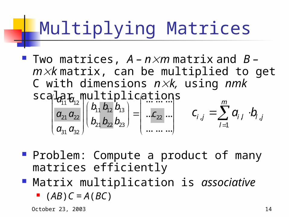
Two matrices, A – nm matrix and B – mk matrix, can be multiplied to get C with dimensions nk, using nmk scalar multiplications

Problem: Compute a product of many matrices efficiently

Matrix multiplication is associative (AB)C = A(BC)

Multiplying Matrices

, , ,1

m

i j i l l jl

c a b

11 12

1311 1221 22 22

2321 2231 32

... ... ...

... ...

... ... ...

a abb b

a a cbb b

a a

October 23, 2003 15

Multiplying Matrices (2)

The parenthesization matters Consider ABCD, where

A is 301,B is 140, C is 4010, D is 1025 Costs:

(AB)C)D1200 + 12000 + 7500 = 20700 (AB)(CD)1200 + 10000 + 30000 = 41200 A((BC)D)400 + 250 + 750 = 1400

We need to optimally parenthesize

1 2 1, where is a matrixn i i iA A A A d d

October 23, 2003 16

Multiplying Matrices (3)

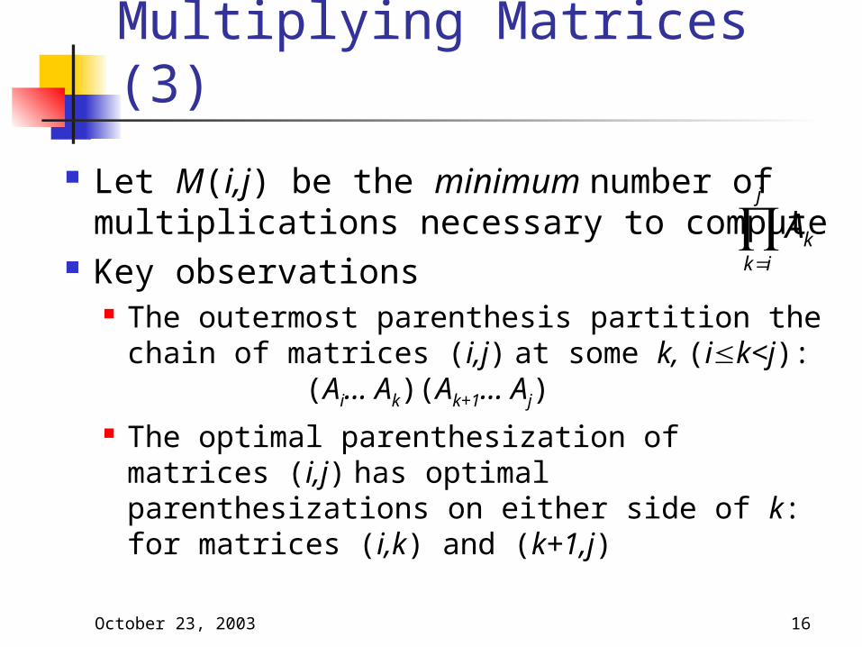
Let M(i,j) be the minimum number of multiplications necessary to compute

Key observations The outermost parenthesis partition the

chain of matrices (i,j) at some k, (ik<j): (Ai… Ak)(Ak+1… Aj)

The optimal parenthesization of matrices (i,j) has optimal parenthesizations on either side of k: for matrices (i,k) and (k+1,j)

j

kk i

A

October 23, 2003 17

Multiplying Matrices (4)

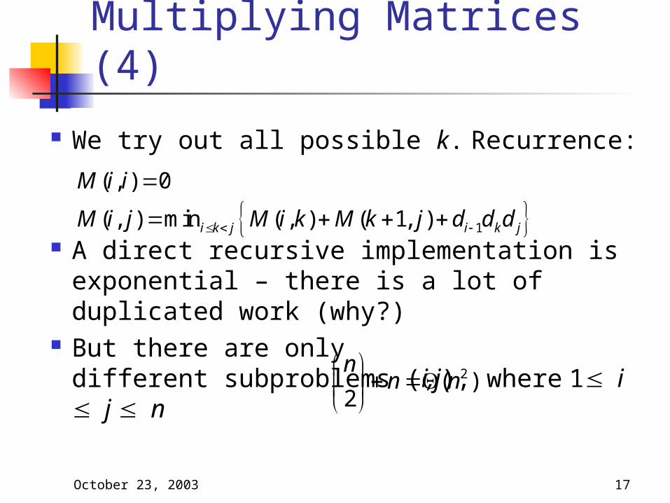
We try out all possible k. Recurrence:

A direct recursive implementation is exponential – there is a lot of duplicated work (why?)

But there are only different subproblems (i,j), where 1i j n

1

( , ) 0

( , ) min ( , ) ( 1, )i k j i k j

M i i

M i j M i k M k j d d d

2( )2

nn n

October 23, 2003 18

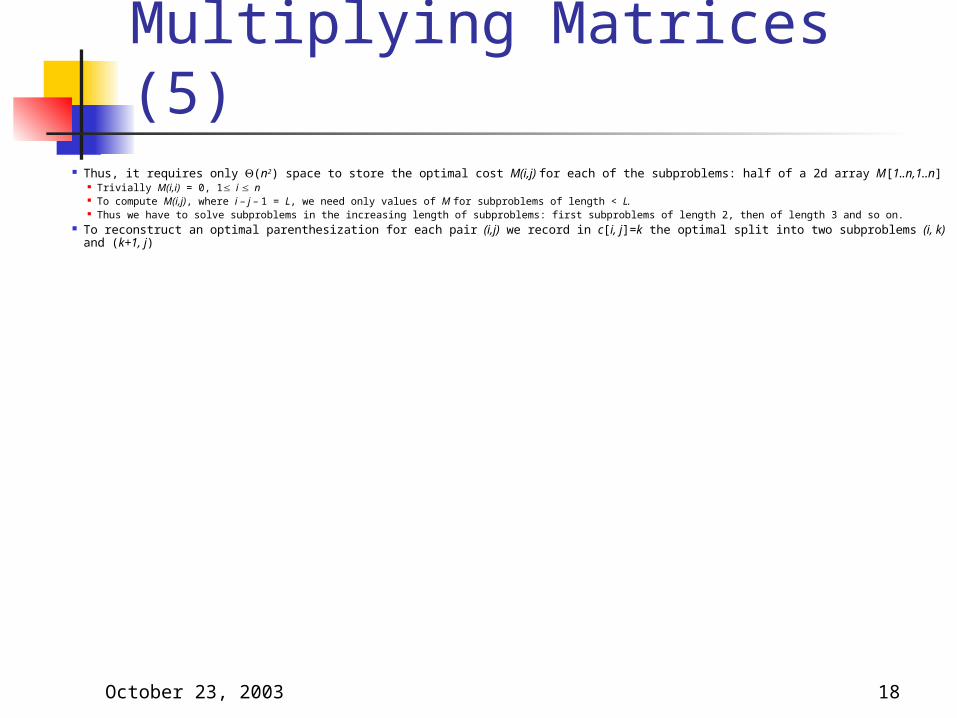
Multiplying Matrices (5) Thus, it requires only (n2) space to store the optimal cost M(i,j) for each of the subproblems: half of a 2d array M[1..n,1..n]

Trivially M(i,i) = 0, 1i n To compute M(i,j), where i – j – 1 = L, we need only values of M for subproblems of length < L. Thus we have to solve subproblems in the increasing length of subproblems: first subproblems of length 2, then of length 3 and so on.

To reconstruct an optimal parenthesization for each pair (i,j) we record in c[i, j]=k the optimal split into two subproblems (i, k) and (k+1, j)

October 23, 2003 19

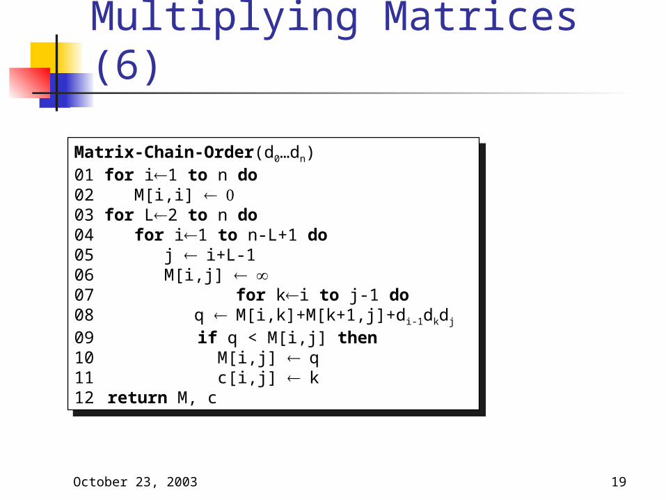
Multiplying Matrices (6)

Matrix-Chain-Order(d0…dn)01 for i1 to n do02 M[i,i] 03 for L2 to n do04 for i1 to n-L+1 do05 j i+L-106 M[i,j] 07for ki to j-1 do08 q M[i,k]+M[k+1,j]+di-1dkdj

09 if q < M[i,j] then10 M[i,j] q11 c[i,j] k12 return M, c

Matrix-Chain-Order(d0…dn)01 for i1 to n do02 M[i,i] 03 for L2 to n do04 for i1 to n-L+1 do05 j i+L-106 M[i,j] 07for ki to j-1 do08 q M[i,k]+M[k+1,j]+di-1dkdj

09 if q < M[i,j] then10 M[i,j] q11 c[i,j] k12 return M, c

October 23, 2003 20

Multiplying Matrices (7)

After the execution: M [1,n] contains the value of an optimal solution and c contains optimal subdivisions (choices of k) of any subproblem into two subsubproblems

Let us run the algorithm on the four matrices:A1 is a 2x10 matrix,

A2 is a 10x3 matrix,

A3 is a 3x5 matrix, and

A4 is a 5x8 matrix.

October 23, 2003 21

Multiplying Matrices (8)

Running time It is easy to see that it is O(n3) It turns out, it is also (n3)

From exponential time to polynomial

October 23, 2003 22

Memoization If we still like recursion very much, we can

structure our algorithm as a recursive algorithm: Initialize all M elements to and call Lookup-

Chain(d, i, j)Lookup-Chain(d,i,j)1 if M[i,j] < then2 return m[i,j]3 if i=j then4 m[i,j] 0 5 else for k i to j-1 do6 q Lookup-Chain(d,i,k)+

Lookup-Chain(d,k+1,j)+di-1dkdj

7 if q < M[i,j] then8 M[i,j] q9 return M[i,j]

Lookup-Chain(d,i,j)1 if M[i,j] < then2 return m[i,j]3 if i=j then4 m[i,j] 0 5 else for k i to j-1 do6 q Lookup-Chain(d,i,k)+

Lookup-Chain(d,k+1,j)+di-1dkdj

7 if q < M[i,j] then8 M[i,j] q9 return M[i,j]

October 23, 2003 23

Memoization (2)

Memoization: Solve the problem in a top-down fashion,

but record the solutions to subproblems in a table.

Pros and cons: Recursion is usually slower than loops

and uses stack space Easier to understand If not all subproblems need to be solved,

you are sure that only the necessary ones are solved

October 23, 2003 24

Dynamic Programming

In general, to apply dynamic programming, we have to address a number of issues: 1. Show optimal substructure – an optimal

solution to the problem contains within it optimal solutions to sub-problems

Solution to a problem: Making a choice out of a number of possibilities (look

what possible choices there can be) Solving one or more sub-problems that are the result of

a choice (characterize the space of sub-problems) Show that solutions to sub-problems must themselves

be optimal for the whole solution to be optimal (use “cut-and-paste” argument)

October 23, 2003 25

Dynamic Programming (2) 2. Write a recurrence for the value of an

optimal solution Mopt = Minover all choices k {(Combination (e.g., sum)

of Mopt of all sub-problems, resulting from choice k) + (the cost associated with making the choice k)}

Show that the number of different instances of sub-problems is bounded by a polynomial

October 23, 2003 26

Dynamic Programming (3) 3. Compute the value of an optimal solution

in a bottom-up fashion, so that you always have the necessary sub-results pre-computed (or use memoization)

See if it is possible to reduce the space requirements, by “forgetting” solutions to sub-problems that will not be used any more

4. Construct an optimal solution from computed information (which records a sequence of choices made that lead to an optimal solution)

October 23, 2003 27

Longest Common Subsequence

Two text strings are given: X and Y There is a need to quantify how

similar they are: Comparing DNA sequences in studies of

evolution of different species Spell checkers

One of the measures of similarity is the length of a Longest Common Subsequence (LCS)

October 23, 2003 28

LCS: Definition

Z is a subsequence of X, if it is possible to generate Z by skipping some (possibly none) characters from X

For example: X =“ACGGTTA”, Y=“CGTAT”, LCS(X,Y) = “CGTA” or “CGTT”

To solve LCS problem we have to find “skips” that generate LCS(X,Y) from X, and “skips” that generate LCS(X,Y) from Y

October 23, 2003 29

LCS: Optimal Substructure

We make Z to be empty and proceed from the ends of Xm=“x1 x2 …xm” and Yn=“y1 y2 …yn” If xm=yn, append this symbol to the beginning of Z,

and find optimally LCS(Xm-1, Yn-1) If xmyn,

Skip either a letter from X or a letter from Y Decide which decision to do by comparing LCS(Xm, Yn-1)

and LCS(Xm-1, Yn)

“Cut-and-paste” argument

October 23, 2003 30

LCS: Reccurence The algorithm could be easily extended by

allowing more “editing” operations in addition to copying and skipping (e.g., changing a letter)

Let c[i,j] = LCS(Xi, Yj)

Observe: conditions in the problem restrict sub-problems (What is the total number of sub-problems?)

0 if 0 or 0

[ , ] [ 1, 1] 1 if , 0 and

max{ [ , 1], [ 1, ]} if , 0 and i j

i j

i j

c i j c i j i j x y

c i j c i j i j x y

October 23, 2003 31

LCS: Compute the Optimum

LCS-Length(X, Y, m, n)1 for i1 to m do2 c[i,0] 03 for j0 to n do4 c[0,j] 05 for i1 to m do6 for j1 to n do7 if xi = yj then8 c[i,j] c[i-1,j-1]+19 b[i,j] ”copy”10 else if c[i-1,j] c[i,j-1]

then11 c[i,j] c[i-1,j]12 b[i,j] ”skipX”13 else14 c[i,j] c[i,j-1]15 b[i,j] ”skipY”16 return c, b

LCS-Length(X, Y, m, n)1 for i1 to m do2 c[i,0] 03 for j0 to n do4 c[0,j] 05 for i1 to m do6 for j1 to n do7 if xi = yj then8 c[i,j] c[i-1,j-1]+19 b[i,j] ”copy”10 else if c[i-1,j] c[i,j-1]

then11 c[i,j] c[i-1,j]12 b[i,j] ”skipX”13 else14 c[i,j] c[i,j-1]15 b[i,j] ”skipY”16 return c, b

October 23, 2003 32

LCS: Example

Lets run: X =“GGTTCAT”, Y=“GTATCT”

What is the running time and space requirements of the algorithm?

How much can we reduce our space requirements, if we do not need to reconstruct an LCS?

October 23, 2003 33

Next Lecture

Graphs: Representation in memory Breadth-first search Depth-first search Topological sort