Embed Size (px)
Citation preview


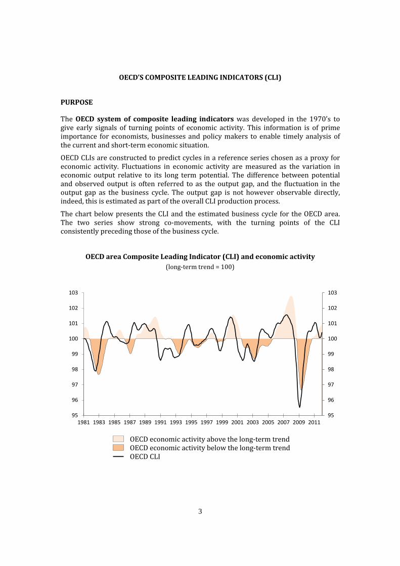
6
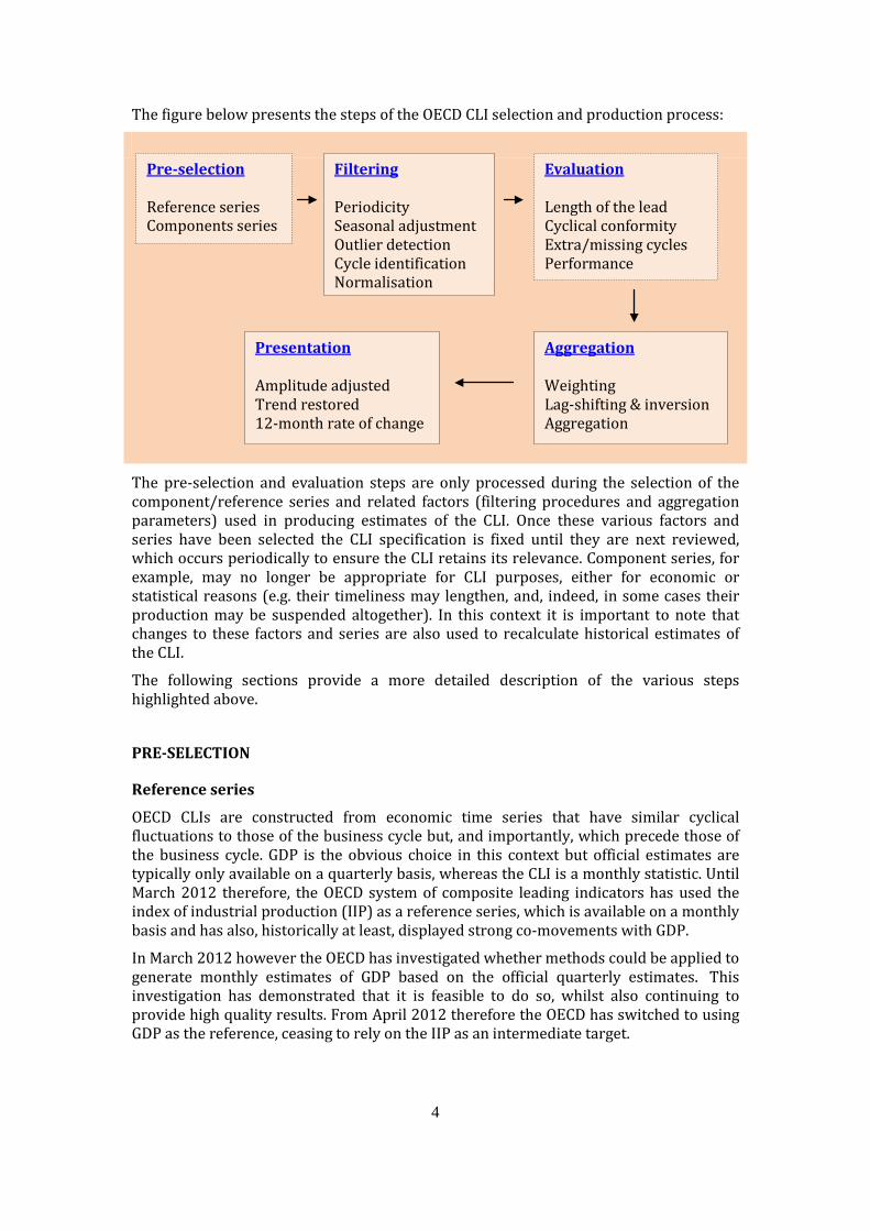
FILTERING
Once the leading components have been selected the second (and first step of production) begins. This step attempts to remove factors, such as seasonal patterns, outliers, trends etc that may obscure the underlying cyclical patterns in the component series, using what are referred to as a sequence of filters. Each of these factors, and the approaches used to identify and remove them, are described below.
Periodicity
OECD composite leading indicators are published monthly and are largely composed using monthly leading component series. Some of the component series are, however, only available on a quarterly basis, and these need to be converted to a monthly frequency. This conversion from quarterly to monthly is achieved via linearly interpolating quarterly series and aligning them with the most appropriate month of the quarter, depending on the nature/construction of the quarterly series. For most series this is the central month of the quarter but where quarterly dates refers to the end of the period, the final month of the quarter is aligned, and for quarterly series based on surveys conducted in a given month of the quarter, the month itself is aligned.
Seasonal adjustment
Many of the component series used in the CLI system are seasonally adjusted by the source provider, usually statistical offices. This is not the case however for all component series. In these cases, seasonal adjustments are made using either the X12 or TRAMO/SEATS methods2
Outlier detection
.
Outliers are observations in component series that lie outside the normal range of expected observations. Often their cause is identifiable: for example, a strike, a change in regulation, etc.
The OECD system of leading indicators utilises the TRAMO module of the TRAMO/SEATS seasonal adjustment procedure3
Cycle identification (de-trending, smoothing and turning points detection)
to identify outliers in each series. After the location and nature of the outliers identified, the outliers are replaced by an estimated value, the process for which varies depending on whether the outliers reflect: (i) additive outliers (caused by a temporary shock); (ii) transitory changes (also caused by temporary shocks but where observations return to normal after several periods); and (iii) level shifts (consequence of a permanent shock). In addition TRAMO can also provide estimates in cases of missing values.
The next step in the filtering process is to identify the underlying cyclical pattern of the component indicator. This requires the removal of two factors: long term trends and high frequency noise. The process of removing these factors can be performed in a single step (referred to as band-pass filtering), or separated into distinct steps for trend removal and smoothing.
2 http://circa.europa.eu/irc/dsis/eurosam/info/data/demetra.htm 3 For further information see “Brief description of the TRAMO-SEATS methodology”, in Modelling Seasonality and Periodicity, Proceedings of the 3rd International Symposium on Frontiers of Time Series Modelling, the Institute of Statistical Mathematics, Tokyo, 2002.
7
De-trending and Smoothing
Up until November 2008 the OECD CLI system determined the long-term trend using the Phase Average Trend method (PAT) developed by the US National Bureau of Economic Research. Series smoothing was conducted using the Month for Cyclical Dominance (MCD) method. Following a study4
For more information on the de-trending methods mentioned above see
undertaken in 2008 that compared the revision properties of PAT, the Hodrick-Prescott filter and the Christiano-Fidgerald filter, the OECD has decided to replace the combined PAT/MCD approach with the Hodrick-Prescott filter. This change not only improves the stability of the cyclical estimates, but also makes the CLI production process more transparent and delivers greater operational stability.
annex A
Before the HP filter is applied the TRAMO module is applied to component series to determine whether they should be modelled as additive or multiplicative series, and to provide short horizon stabilizing forecasts. Multiplicative series are subject to a log-transformation, after which they can be processed in the same way as additive series. Once this has been determined the HP-filter is run as a band-pass filter with parameters set, such that the frequency cut-off occurs at frequencies higher than 12-months and lower than 120 months.
Turning Point Detection
The algorithm currently used to detect turning-points is a simplified version of the Bry-Boschan algorithm. It selects local minima and maxima in the cyclical part of the series, but, at the same time, enforces minimum phase length and minimum cycle length conditions, and ensures the alternation of troughs and peaks. For further details on turning point estimation see Annex B.
The identification of turning-points is also an important criterion used in determining whether component indicators have suitable leading properties, (used mainly in the evaluation stage).
Normalisation
Naturally, even after the above steps have been conducted, the different component series used in the construction of a single composite indicator will be expressed in different units or scales. As such, the various component series that are used in the construction of a CLI are first normalised. This normalisation process is achieved by subtracting from ‘filtered’ observations the mean of the series, and dividing this by the mean absolute deviation of the series, and, finally, by adding 100 to each observation.
EVALUATION
This step is only part of the selection process of the CLI and does not apply to the regular monthly CLI calculation and update routine.
The pre-selected candidate component series are evaluated for their cyclical performance using a set of statistical methods. The OECD system of composite leading indicators examines the cyclical behaviour of each candidate component series in
4 http://www.oecd.org/dataoecd/32/13/41520591.pdf

8
relation to the cyclical turning points of the reference series, i.e. peak-and-trough analysis. This assessment is summarised below:
Length and consistency of the lead
Lead times are measured in months, reflecting the time that passes between turning points in the component and reference series. Of course lead times vary from turning point to turning-point but the aim is to construct leading indicators whose lead times are on average between 6 to 9 months and that have relatively small variances. To evaluate the length of leads, both mean and median leads are used, because the mean lead on its own can be strongly affected by outliers. The consistency of leads is measured by the standard deviation from the mean lead.
Cyclical conformity between selected indicators and reference series
If the cyclical profiles are highly correlated, the indicator will provide a signal, not only to approaching turning points, but also to developments over the whole cycle. The cross correlation function between the reference series and the candidate components (or the composite leading indicator itself) provides invaluable information on cyclical conformity. The location of the peak of the cross correlation function is a good alternative indicator of average lead time. Whereas the correlation value at the peak provides a measure of how well the cyclical profiles of the indicators match, the size of correlations cannot be the only indicators used for component selection.
As a cross-check the average lead of the cyclical indicator, measured by the lag at which the closest correlation occurs, should not be too different from the median lag if the composite leading indicator is to provide reliable information about approaching turning points and the evolution of the reference series.
Missing or extra cycles
Clearly selected component indicators should not flag extra cycles or, moreover, miss any cycles compared to the reference series. Indeed, if too many extra cycles are flagged, the risk that the CLI gives false signals becomes significant. Equally, if the CLI failed to predict several cycles in the past it is unlikely to be reliable in anticipating changes in the future.
Performance
After selection the component indicators are combined and aggregated into various composite indicators. The best performing composite indicator is selected based on the same assessment criteria described above.
AGGREGATION
Weighting
Component indicators used in constructing any composite leading indicator have equal-weights. But for zone aggregates the CLIs themselves are weighted reflecting country weights: for more information see the OECD CLI zone aggregation methodology (http://www.oecd.org/dataoecd/56/25/38873830.pdf)
It is important to note however that the normalisation procedure, described above, introduces an implicit weighting of component series, with the series being weighted by the inverse of their mean absolute deviation.
9
Lag-shifting and inversion
Having a reference series means having a reference chronology to classify the timing of series as either:
• leading (movements precede those of the reference series), • coincident (movements coincide with those of the reference series), or • lagging (movements follow those of the reference series)
In this respect, the following classification system is used in the CLI:
Type of behaviour at turning points Median lead/lag
Coincident between +/- 2 months Leading: shorter/medium longer
Between 2 months to 8 months over 8 months
Lagging -2 months or less It is important to note that some component series may have counter-cyclical (inverse) behaviour compared to the reference series. But such characteristics can be as useful in the CLI construction as pro-cyclical series.
Lag-shifting is a new feature incorporated into the process. It reflects the lagging of the different selected component series for a given CLI such that, in practice, the lead-times of the component series align with each other, thus maximising the intensity of turning points in the CLI.
Aggregation
Aggregation of component indicators is clearly done with a view to improving the predictive capacity of the overall composite indicator. But some complications can arise in aggregation reflecting the availability of data for component series, both historical and current. As a rule therefore, for any given period, a CLI is only calculated if data for 60% or more of the component series are available in that period.
The aggregation is done by averaging the growth rates of each component indicator. Then, the average growth rates are chained to form the final indicator. The advantage of this procedure is that the CLI is less sensitive to missing or late arriving component data.
PRESENTATION
CLIs can be presented in several forms, reflecting, in the main, user needs. The following forms are all produced in the OECD CLI system:
The amplitude adjusted CLI vs. the de-trended reference series
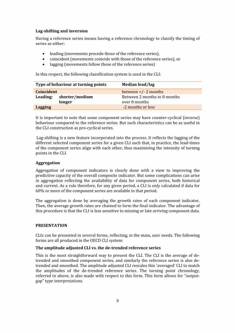
This is the most straightforward way to present the CLI. The CLI is the average of de-trended and smoothed component series, and similarly the reference series is also de-trended and smoothed. The amplitude adjusted CLI rescales this ‘averaged’ CLI to match the amplitudes of the de-trended reference series. The turning point chronology, referred to above, is also made with respect to this form. This form allows for “output-gap” type interpretations.
10
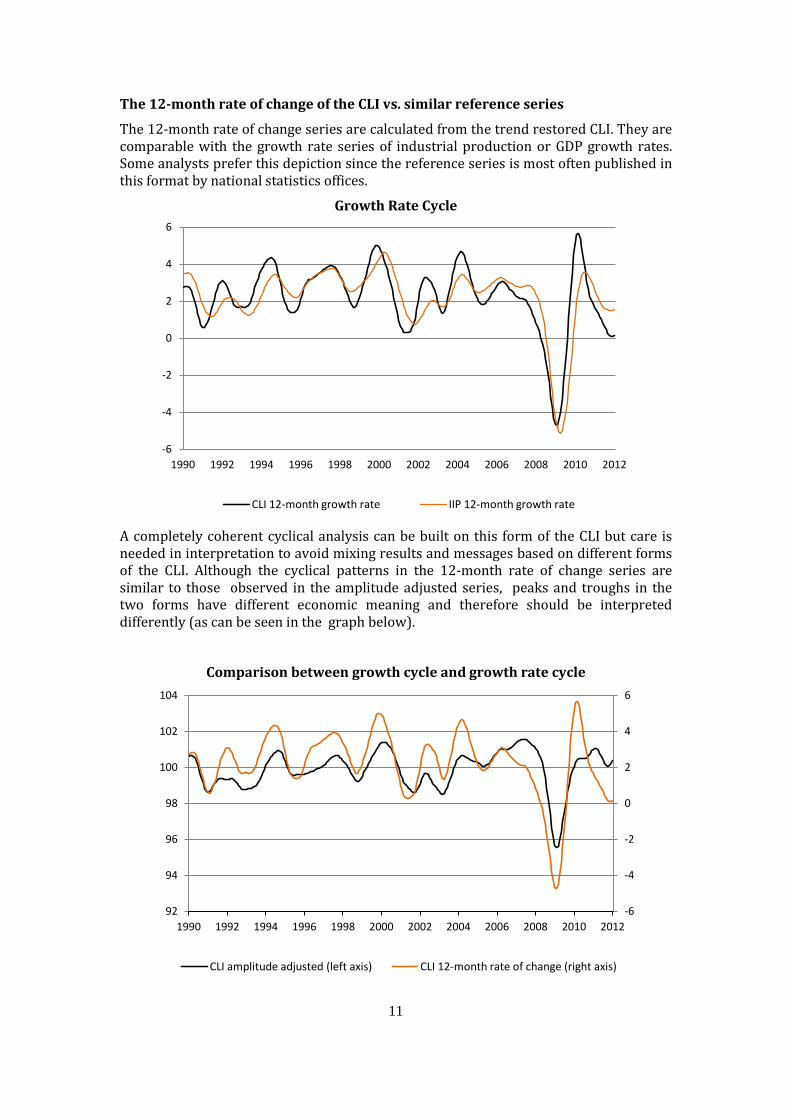
Growth Cycle
The trend restored CLI vs. the original reference series
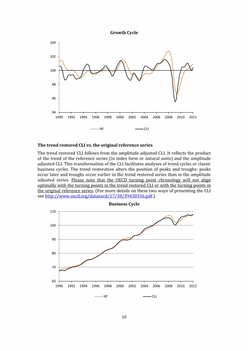
The trend restored CLI follows from the amplitude adjusted CLI. It reflects the product of the trend of the reference series (in index form or natural units) and the amplitude adjusted CLI. This transformation of the CLI facilitates analyses of trend cycles or classic business cycles. The trend restoration alters the position of peaks and troughs: peaks occur later and troughs occur earlier in the trend restored series than in the amplitude adjusted series. Please note that the OECD turning point chronology will not align optimally with the turning points in the trend restored CLI or with the turning points in the original reference series. (For more details on these two ways of presenting the CLI see http://www.oecd.org/dataoecd/17/38/39430336.pdf.).
Business Cycle
94
96
98
100
102
104
1990 1992 1994 1996 1998 2000 2002 2004 2006 2008 2010 2012
IIP CLI
60
70
80
90
100
110
1990 1992 1994 1996 1998 2000 2002 2004 2006 2008 2010 2012
IIP CLI


16
Christiano-Fidgerald (CF) filter
The Christiano-Fitzgerald random walk filter is a band pass filter that was built on the same principles as the Baxter and King (BK) filter. These filters formulate the de-trending and smoothing problem in the frequency domain. With continuous and/or infinitely long time series the frequency filtering would be an exact procedure. However the discrete nature of data do not allow for such perfection. Both the BK and CF filters approximate the ideal infinite band pass filter. The Baxter and King version is a symmetric approximation, with no phase shifts in the resulting filtered series. But symmetry and phase correctness comes at the expense of series trimming. Depending on the trim factor a certain number of values at the end of the series cannot be calculated. There is a trade-off between the trimming factor and the precision with which the optimal filter can be approximated. On the other hand, the Christiano-Fitzgerald random walk filter uses the whole time series for the calculation of each filtered data point. The advantage of the CF filter is that it is designed to work well on a larger class of time series than the BK filter, converges in the long run to the optimal filter, and in real time applications outperforms the BK filter. For details see Christiano-Fitzgerald [1999]. For these reasons we included only the Christiano-Fitzgerald filter in our study that compares different cycle detection methods.
The CF filter is a steep, asymmetric filter that converges in the long run to the optimal filter. It can be calculated as follows:
∑ −
=
−−−−−−−+
−−=
==−
=≥−
=
++++++++=
1
10
0
,11221111110
21~
2,2, and,1,)sin()sin(where~...~...
k
j jk
luj
tttTtTTtTttt
BBB
pb
paabBj
jjajbB
yByByByByByByBcππ
ππ
The parameters pu and pl are the cut-off cycle length in month. Cycles longer than pl and shorter than pu are preserved in the cyclical term ct.