Ohio Forests2006

Resource Bulletin

NRS-36

2009

Northern

Research Station

United States Department of Agriculture

ForestService

Thomas AlbrightDavid BergerPhil BergsrudTodd BixbyAmy CalehuffAarron ClarkJames ConnollyChris CoolbaughGene DresselyMichael EffingerAdrienne EvansScott GarberTed GoodnightJason GouldRobert GregoryMarlin GruverJohn HighamScott HoptonRobert IlgenfritzKatherine JohnsonPaul KelleyJoe KernanKaren KublyNick LarsonJohanna LeonardChris MateErica MattsonRichard McculloughCade MitchellWilliam MoirPaul Natiella

Paul NeubauerAdrienne OryhonKevin PackardAnne PaulsonStephen PawlowskiMark PeetMitch PennabakerJon PorierStephen PotterMatt PowellAnn QuinionKirk RamseyJason ReedTodd RenningerNatalie RobisonTodd RoffeBrian RuddDoug SchwemleinRichard StarrBruce StephensLeland SwogerJeff TilleyKathryn TillmanBryan TirrellJeffrey WazeneggerMike WhitehillThomas WillardRon YaworskyJessica YeagleAshley ZickefooseLewis Zimmerman

Acknowledgments—Ohio Inventory Crew Members, 2001-2006

Visit our homepage at: http://www.nrs.fs.fed.us/

Published by: For additional copies:

U.S. FOREST SERVICE U.S. Forest Service11 CAMPUS BLVD., SUITE 200 Publications DistributionNEWTOWN SQUARE, PA 19073-3294 359 Main Road Delaware, OH 43015-8640September 2009 Fax: 740-368-0152

Manuscript received for publication 10 November 2008.

Cover Photo

Scioto Trail. Photo used with permission by the Ohio Department of Natural Resources, Division of Forestry.

Ohio Forests2006

Richard H. Widmann, Dan Balser, Charles Barnett, Brett J. Butler, Douglas M. Griffith,

Tonya W. Lister, W. Keith Moser, Charles H. Perry, Rachel Riemann, and Christopher W. Woodall

Foreword

Forests at a tipping point

Ohio’s forests are a critical component of the state’s natural resources. Covering nearly 8 million acres, or 30 percent of the state, these diverse forests support important biological communities and create habitat for wildlife, forest products, clean water, and opportunities for recreation. Essential to making sound decisions about Ohio’s forests is credible information. Forest Inventory and Analysis (FIA) data help fill this need. Such data tell us where we are and where we are going, and they provide the basis for making informed decisions about how we can sustain our forests for future generations.

The fifth inventory of Ohio’s forests suggests that we are at a tipping point. Ohio’s forests hold more wood, provide more wildlife habitat, and store more carbon than 15 years ago. Yet, for the first time since the 1940s, the acreage of Ohio’s forest land has not increased, and some parts of the state have seen large losses in forest cover. More Ohioans than ever own forest land and enjoy the many benefits that forests provide. But, as Ohio’s forest lands are subdivided and fragmented, the ability of these forests to provide timber, wildlife habitat, recreation, and solitude is reduced. Oak-hickory forests make up over one-half of the state’s forests. Oaks as seedlings and saplings, however, have declined in abundance, and oaks will likely play a smaller role in Ohio’s future forests. The quality and value of our timber has increased during the past 15 years, and landowners intend to harvest trees on one-fifth of Ohio’s forested acres in the next 5 years. However, only 4 percent of forest landowners have a formal management plan for their forests, and fewer than one in seven seeks any sort of advice before making decisions that will affect them and their forests for decades.

John F. Kennedy said: "It is our task in our time and in our generation, to hand down undiminished to those who come after us, as was handed down to us by those who went before, the natural wealth and beauty which is ours." The data presented in this report clearly highlight the challenges our forests face: fragmentation, uninformed management, loss of oak, invasive species, and a host of other concerns. How we address these concerns, how we balance forest conservation and sustainable use, will determine the forests that future generations experience and the benefits they receive. Doubtless, the FIA reports of tomorrow will document the successes, or the failures, of the choices we make today.

David Lytle, Ph.D.,State Forester and Chief,Ohio Department of Natural Resources, Division of Forestry

Contents

Introduction ........................................................................................................... 1Highlights ............................................................................................................... 2 On the Plus Side .............................................................................................. 2 Issues to Watch ................................................................................................ 4

Forest Land Features .............................................................................................. 7 Dynamics of the Forest Land Base ................................................................. 8 Potential Productivity and Availability of Forest Land ................................. 12 Ownership of Forest Land .............................................................................14 Urbanization and Fragmentation of Forest Land ......................................... 22

Forest Resource Attributes .................................................................................. 27 Forest Structure—How Dense are the Woods? .............................................. 28 Numbers of Trees by Diameter Class ............................................................ 33 Tree Condition—Crown Position and Live Crown Ratio ............................ 37 Forest Composition ....................................................................................... 39 Distribution of Common Species ................................................................. 43 Volume of Growing-stock Trees .................................................................... 45 Variation in Hardwood Quality by Species .................................................. 52 Biomass Volume of Live Trees ...................................................................... 54 Components of Annual Volume Change ..................................................... 57 Mortality ........................................................................................................ 60 Status of Oaks ................................................................................................ 62 Important Habitat Features ........................................................................... 65

Forest Health Indicators ...................................................................................... 69 Down Woody Material .................................................................................. 70 Lichens ........................................................................................................... 73 Forest Soils ..................................................................................................... 78 Vascular Plants in Ohio’s Forest ................................................................... 83

Threats to the Health of Important Tree Species in Ohio ................................ 90 American Beech ............................................................................................. 92 Oak ................................................................................................................ 95 Ash ................................................................................................................. 98 Elm ................................................................................................................101

Timber Products ................................................................................................ 103Data Sources and Techniques ............................................................................107 Forest Inventory ........................................................................................... 108 National Woodland Owner Survey .............................................................110 Timber Products Inventory ..........................................................................110

Glossary ...............................................................................................................111Literature Cited...................................................................................................119

1

Introduction

This is the fifth inventory of Ohio’s forests, the first using a new annualized inventory system. Previous inventories were completed for 1952 (Hutchison and Morgan 1956), 1968 (Kingsley and Mayer 1970), 1979 (Dennis and Birch 1981), and 1991 (Griffith et al. 1993). These inventories provided a snapshot of the forest for specific periods in time after which no new information was available until the next full inventory of the State. Henceforth, inventory data for the State will be updated annually and full remeasurement of all inventory plots will occur every 5 years. FIA landscape-level information is the only forest inventory that uses a permanent network of ground plots. Data are collected consistently across the Nation enabling comparisons among states and regions. Having current inventory information always available should help in making better decisions about Ohio forests and planning for the future.

Maintaining openings to improve wildlife habitat on the Wayne National Forest; photo by Kari Kirschbaum, U.S. Forest Service

2

Ohio’s forests have doubled in area since the 1942 inventory to now total 7.9 million acres and cover 30 percent of the State’s land.

Ninety-seven percent of Ohio’s forest land is classified as productive

timberland and potentially available for timber harvesting.

Public ownership of forest land has steadily increased, tripling since 1952.

Publicly owned forests now total 952,500 acres or 12 percent of the State’s

forest land.

Representing the largest ownership category, family forest owners hold 5.8

million acres—accounting for 73 percent of the State’s forest land.

Most stands are well stocked with trees of commercial importance. Since

1991, stocking levels have increased as acreage has shifted to fully stocked

and overstocked levels.

Since 1991, numbers of trees in the larger diameter classes have continued to

increase while numbers of trees have decreased in the 6- and 8-inch classes.

There are few areas in Ohio where any one species represents more than half

the stocking of live trees. This diverse mix of species reduces the impact of

insects and diseases that target a single tree species.

The current growing-stock inventory is the highest recorded in Ohio since

FIA began. Growing-stock volume totals 12.3 billion cubic feet, which is 22

percent more than in 1991 and averages 1,603 cubic feet per acre.

Timber growth is concentrated on sawtimber-size trees (more than 11 inches

in d.b.h.). Since 1991 the saw log portion of growing-stock volume increased

by 35 percent to 41 billion board feet.

Yellow-poplar continues to lead in volume followed by red maple and sugar

maple.

Highlights

On the Plus Side

3

Volume increases for the maples are larger than for the oaks, although all species of oak increased in

volume.

The portion of sawtimber volume in high-quality tree grades 1 and 2 increased from 32 percent in 1991 to

43 percent in 2006.

Ohio’s forests are accumulating substantial amounts of biomass. These stores of carbon will receive more

attention as we seek sources for renewable energy and ways to offset carbon dioxide emissions.

During the last 50 years in Ohio, the growth of trees has greatly outpaced mortality and removals. The

growth-to-removals ratio averaged 2:1 for 1991-2006.

Net growth exceeded removals for all major species except elm, which had negative growth due to high

mortality.

The high growth-to-removals ratios for red maple, sugar maple, and yellow-poplar show these species will

increase in importance in Ohio’s forests.

Tree mortality rates in Ohio have increased since previous inventories, although they are still comparable to

those in surrounding states.

Because hard mast production increases as trees become larger, we can assume that hard mast production

has increased in Ohio because of increases in the number of large-diameter oaks and hickories.

The down woody fuel loadings in Ohio’s forests are neither exceedingly high nor different from those

found in neighboring states.

A total of 92 million cubic feet of wood was harvested from Ohio’s forests in 2006 and used for products.

Although this total is nearly the same amount as the 1989 harvest, production shifted from pulpwood to

saw logs.

Markets for saw logs in Ohio have been strong as indicated by a stable harvest from Ohio’s forests and a

continuation of log imports surpassing exports.

4

Issues to Watch Trends in land use change indicate that the area of forest land in Ohio may be near a peak.

The large amount of forest land in small private holdings makes the delivery of government programs difficult and forest management less economical. These difficulties will likely be exacerbated by further parcelization of Ohio’s forest land, which is indicated by increasing numbers of owners and increases in acreage in holdings of fewer than 50 acres.

The turnover of forest land to an increasing number of new owners will create a need for more education, advice, and other services to family forest owners.

The combination of increasing numbers of forest land owners owning smaller parcels of land (parcelization), decreasing forest patch sizes (fragmentation), and increasing proximity to human populations, roads, and other urban areas (urbanization) is making forest land more difficult to manage for timber and wildlife as well as making traditional access to forests for recreation more difficult.

More than half of Ohio’s forest land occurs in census blocks with more than 50 people per square mile.

The 2.0 million acres (13 percent) of timberland that are poorly stocked with commercially important species represent a loss of potential growth, although these forests still contribute to forest diversity.

Shaded conditions created by overstory trees are stressing a large portion of trees below 10 inches in diameter. Most trees in the 2-, 4-, 6-, and 8-inch diameter classes are in an overtopped or intermediate crown position.

In the current inventory, oaks represent more than one-third of the trees 20 inches and larger in diameter, but only 5 percent of trees in the 2- and 4- inch diameter classes.

5

A lack of oaks in the small diameter classes means that as large oaks are harvested or die, they likely will be replaced by species such as red and sugar maples that dominate the lower diameter classes.

Future losses of oaks will affect wildlife populations and wood-using industries that now depend on oak.

Future tree quality may be affected by changes in species composition. Red and sugar maples had some of the largest increases in volume but typically grade poorer than other major species.

Nearly a third of removals are due to conversion of timberland to nonforest uses, which threatens sustainability because such changes are usually permanent.

American beech mortality is expected to increase significantly as the beech scale insect spreads by about 9.1 miles/year.

Future defoliation events caused by the gypsy moth caterpillar and the potential arrival of Sudden Oak Death in the eastern United States are of particular concern to the oak resource in Ohio.

Emerald ash borer, a lethal pest found in Ohio, will increase ash mortality in both urban and forested landscapes. It will likely cause significant financial costs to municipalities, property owners, and the forest products industries in the State.

Because white ash is the leading species in the Northwestern and Southwestern geographic units of the State, future mortality caused by the emerald ash borer will likely be significant in these areas.

FOREST LAND FEATURES

Hocking Hills State Park; photos by Richard Widmann, U.S. Forest Service

8

FEATURES

The amount of forest land in Ohio and percentage of land under forest cover are

crucial measures in assessing forest resources and are vital for making informed

decisions about forests. These measures are the foundation for estimating numbers of

trees, wood volume, and biomass. Trends in forest land area are an indication of forest

sustainability, ecosystem health, and land use practices. Gains and losses in forest

area directly affect the ability of forests to provide goods and services, including wood

products, wildlife habitat, recreation, watershed protection, and more.

FIA groups counties that have similar forest cover, soil, and economic conditions into

geographic units. In Ohio, the Southwestern, Northwestern, and Northeastern Units

are well suited for agriculture and are commonly know as Ohio’s cornbelt and dairy

regions. Terrain in these glaciated units is mostly level to rolling with rich soils. Ohio’s

topography generally becomes rougher from west to east, with the South-Central,

Southeastern, and East-Central Units encompassing Ohio’s hill country. These units

are mostly unglaciated and form the foothills of the Allegheny Mountains to the east.

Ohio forests have doubled in area since 1942 to now total 7.9 million acres, or

30 percent of the State’s land. Successive inventories have shown forest land area

consistently increasing, although the most recent inventory shows a slowing in this

trend. The 100,000-acre increase since 1991 is smaller than past increases and not large

enough to make the 2006 estimate statistically different from 1991 (Fig. 1). Increases

in forest land have corresponded with decreases in farm land. Since 1950, the amount

of land in farms has decreased by 7.2 million acres (includes farm woodlots) (Fig. 2),

while forest land has increased by 2.5 million acres. Although much former farm land

has been developed to meet the needs of a growing population, a substantial portion

has been left untended and has reverted to forest through natural regeneration. These

new forests have increased total forest land in the State and negated losses of forest to

development.

Dynamics of the Forest Land Base

Background

What we found

Ohio farmland; photo by Richard Widmann, U.S. Forest Service

9

FEATURES

Figure 1.—Area of forest land in Ohio by inventory year, 1952, 1968, 1979, and 2006 with approximations of forest land area given for 1900 and 1940 (Kingsley and Mayer 1970) (error bars represent 67-percent confi dence intervals around the estimates).

Figure 2.—Acreage in farms (includes farm woodlots), Ohio, 1950-2005 (source: National Agriculture Statistics Service).

3

4

5

6

7

8

9

1890 1900 1910 1920 1930 1940 1950 1960 1970 1980 1990 2000 2010

Year

Mill

ion

Acr

es

0

5

10

15

20

25

1950 1960 1970 1980 1990 2000

Year

Mill

ion

Acr

es

21.8

14.6

10

FEATURES

Figure 3.—Distribution of forest land in Ohio based on the Multi-Resolution Land Characteristics project, 1992. The MRLC uses data from the Landsat satellite to map land across the Nation.

The percentage of land in forest cover increases from northwest to southeast in Ohio

(Fig. 3, 4). The East-Central, Southeastern, and South-Central Units account for two-

thirds of the State’s forest land. Gains in forest land occurred in the Northeastern,

East-Central, Southeastern, and Southwestern Units of the State; decreases occurred in

the Northwestern and South-Central Units (Fig. 5). The Northwestern Unit is the least

forested portion of the State and has lost the largest percentage of forest acreage since

1991.

Across the State, losses of forest land due to development have been more than offset

by gains in forest land because of abandoned farm land reverting to forests. Because

of increased development and a slowing in farm land losses, recent changes in total

forest land have been small. These trends may indicate that the area of forest land in

Ohio is peaking. Future changes in Ohio’s forest land will depend on the pace of land

development and to a great extent on the economics of farming. Small percentage

changes in the area of nonforest land can significantly affect forest land area, especially

in sparsely forested areas like Ohio’s Northwestern Unit. Recent proposals to increase

agricultural biofuels, such as growing switchgrass as feed stock for ethanol production,

may promote the conversion of forest land to agriculture uses; although long term, the

production of cellulosic ethanol from forests could promote the planting of trees on

agricultural lands.

Forest land

What this means

11

FEATURES

Figure 4.—Acreage of forest land and percentage of land in forest by FIA unit, Ohio, 2006.

Figure 5.—Change in forest land area by FIA unit, Ohio, 1991-2006.

Northwestern717,400 ac10%

Northeastern1,562,500 ac31%

East-Central1,858,000 ac

54%Southwestern

682,900 ac14% Southeastern

1,377,600 ac 67%

South-Central1,720,500 ac

52%

State 7,918,800 ac.30.2%

Approximate extent of glaciation

Northwestern-101,800 ac

-12.4%

Northeastern+69,500 ac

+4.7%

East-Central+112,000 ac

+6.4%Southwestern

+40,200 ac+6.3% Southeastern

+40,400 ac +3.0%South-Central

-25,500 ac-1.5%

State + 134,800 acres+1.7%

12

FEATURES

What this means

Ohio’s forest land is broadly classified into three components that describe the

potential of the land to grow timber products: reserved forest land, timberland, and

other forest land. Two criteria are used to make these designations: site productivity

(productive/unproductive) and reserved status (reserved/unreserved). Forest land

where harvesting is restricted by statute or administrative designation is classified as

reserved forest land regardless of its productivity class. Most land in this category is

in state parks, national parks and recreation areas, and designated natural areas on

the Wayne National Forest. FIA does not use the harvesting intentions of private

owners as a criterion for determining whether forests should be classified as reserved.

Forest land without legal harvesting restrictions and capable of growing trees at a rate

of at least 20 cubic feet per acre (equivalent to about ¼ cord) per year is classified as

timberland. The other forest land category is unreserved and low in productivity. It

is incapable of growing trees at a rate of 20 cubic feet per acre per year. In Ohio, this

includes wet areas where water inhibits tree growth and some strip-mined areas with

extremely degraded soil. These categories help increase our understanding of the

availability of forest resources and in forest management planning.

Ninety-seven percent of Ohio’s forest land, 7.7 million acres, is classified as

timberland, an increase of 57,000 acres since 1991(Fig. 6). However, this increase

is not large enough to make the two estimates statistically different. The amount of

forest land reserved from harvesting has increased with each successive inventory and

now represents 1 percent of the total land area and 3 percent of forest land. Other

forest land is relatively rare and amounts to less than 1 percent of total forest land.

Most of Ohio’s forest land is potentially available for timber harvesting and is

classified as timberland. Because most forest land is classified as timberland, major

trends occurring on timberland also apply to forest land. Additions to reserved forest

land usually come from the reclassification of timberland. But because losses in

timberland to reserved forest land have been small, they have been overwhelmed by

additions to timberland area from agriculture. Trees growing on timberland represent

the resource base upon which the forest products industry relies and are considered

potentially available for harvesting. Discussions later in this report on urbanization

and the woodland owner study provide more details on how much timberland is

actually available and being actively managed for timber products.

Potential Productivity and Availability of Forest Land

Background

What we found

13

FEATURES

Figure 6.—Land area by major use, Ohio, 2006.

Nonforest Land, 18,289,100 ac

70%Other Forest Land,

26,700 ac <1%

Reserved Forest Land, 217,200 ac

1%

Timberland, 7,675,100 ac

29%

30%

Typical stand of saw log size white oak in southeastern Ohio; photo by Richard Widmann, U.S. Forest Service

14

FEATURES

Background How land is managed is primarily the owner’s decision. Owners decide who they will

allow on their land and what types of activities will take place. Therefore, to a large

extent, the availability and quality of forest resources are determined by landowners,

including recreational opportunities, timber, and wildlife habitat. Owners’ decisions

are influenced by their management objectives, size of land holdings, and form of

ownership. Public and private owners often have different goals that reflect their

priorities and management practices. Family forest owners are further influenced

by their age, education, and life experiences. The National Woodland Owner

Survey (NWOS) conducted by the Forest Service studies private forest landowners’

attitudes, management objectives, and concerns. This survey has recently focused on

understanding what is important to family owned forests.

Publicly owned forests represent a relatively small portion of Ohio’s forests. Public

owners hold 952,500 acres, or 12 percent of the State’s forest land. The Federal

Government holds 287,900 acres, amounting to 4 percent of the forest land in the

State (Fig. 7). Included in this are 227,800 acres of forest land in the Wayne National

Forest. The State of Ohio holds 423,000 acres (5 percent) in various state agencies

including state parks and forests, and local governments hold 241,600 acres (3

percent). Public ownership of forest land has steadily increased, tripling since 1952.

Ownership of Forest Land

What we found

State government423,000

5%

Federal government*287,900

4%

Local government241,600

3%

Business & other private**1,170,300

15%

Family forests5,796,000

73%

* Includes 227,800 acres in the Wayne National Forest.

** Includes corporations, non-family partnerships, tribal lands, non-governmental organizations, clubs, and other non-family private groups.

Figure 7.—Ownership of forest land by major ownership category, Ohio, 2006.

15

FEATURES

In Ohio, 345,000 private individuals and enterprises own 88 percent of the State’s

forest land. Of this, businesses hold an estimated 1.2 million acres--15 percent of

the forest land. This category includes corporations, non-family partnerships, tribal

lands, non-governmental organizations, clubs, and other private non-family groups.

Representing the largest ownership category, family forest owners hold 5.8 million

acres, accounting for 73 percent of the State’s forest land.

The NWOS found that there are 336,000 family owned forests in Ohio (Fig. 8). This

category is represented by individuals, farmers, and small family corporations and

partnerships. Ninety-three percent of these owners hold fewer than 50 acres. These

small holdings total 3.2 million acres and make up 55 percent of the family forest

land in the State. Owners with 50 to 100 acres hold 1 million acres and number

15,000. About a quarter of the family forest acreage (1.6 million acres) is held by about

9,000 owners with forested holdings exceeding 100 acres. Since 1991, the number of

owners and acreage in family forest holdings of fewer than 50 acres have increased by

10 and 6 percent, respectively, while the number of owners and acreage in holdings

of 50 acres and larger have decreased (Birch 1996). From a list of 12 reasons for

owning forest land, “part of home or cabin” ranked first by number of ownerships

and “aesthetic enjoyment” ranked first by area owned (Fig. 9). Owning forest land for

194

118

15 90.1 0.1 0.1

1.4

2.4

0.81.0

0.1 0.0 0.00

100

200

300

1-9 10-49 50-99 100-499 500-999 1000-4999 5000+

Size Class of Holdings (acres)

Num

ber o

f Ow

ners

(tho

usan

ds)

0

1

2

3

4

5

6

Acr

es in

Cla

ss (m

illio

ns)

Number of owners (left axis)-- total = 336,000 Acres (right axis)--total = 5,796,000

Figure 8.—Number of family forest owners and acres of forest land by size of forest land holdings, Ohio, 2006.

16

FEATURES

Figure 9.—Percentage of family forest owners and acres of forest land by reasons given for owning forest land ranked as very important or important, Ohio, 2006.

nature protection, as part

of a farm, and for privacy

also ranked high. Timber

production ranked low

in importance to Ohio’s

family forest owners; it

was ranked as important

or very important by only

13 percent of owners who

hold 19 percent of the

acreage. However, 51 percent

of owners holding 60 percent of the family forest land reported harvesting trees and 27

percent of owners had harvested saw logs (Fig. 10).

Written management plans exist on just 8 percent of the family owned forest land,

and only 13 percent of the owners holding 21 percent of the family forest acreage have

sought management advice (Fig. 11). The State Division of Forestry led as a source of

management advice. Family owned forests are frequently associated with a residence or

farm (Fig. 12). Seventy-nine percent of owners with 68 percent of family forest acreage

67 6564

53

19

11

1

5147

35

41

35

19

9

2

13

262829

37

41

19

54

63

5556

0

20

40

60

80

Part of

home,

or ca

bin

Privac

y

Aesthe

tics

Nature

protec

tion

Family

legac

y

Part of

farm

Other r

ecrea

tion

Huntin

g or fi

shing

Land

inve

stmen

t

Firewoo

d prod

uctio

n

Timbe

r prod

uctio

n

Non-tim

ber fo

rest p

roduc

ts

No ans

wer

Reasons (rated very important or important)a

Perc

ent

Ownerships Acres

a Categories are not exclusive.

Field crews get permission before going on private land; U.S. Forest Service, Forest Inventory and Analysis

17

FEATURES

Figure 10.—Percentage of family forest owners and acres of forest land by harvesting experience and products harvested, Ohio, 2006.

51

27

11

3

29

7

17

60

45

22

9

27

8 8

0

20

40

60

80

Any

harve

sting

? "Yes

"

Sawlog

s

Venee

r logs

Pulpwoo

d

Firewoo

dOthe

r

No ans

wer

Perc

ent

Ownerships Acres

Products Harvesteda

a Categories are not exclusive.

Figure 11.—Percentage of family forest owners and acres of forest land who have a written management plan, who have sought advice, and advice source, Ohio, 2006.

21

76 7

5 6

34

01

22344

6

1312

8

1

0

5

10

15

20

25

Have w

ritten

man

agem

ent p

lan

Sough

t adv

ice

State f

orestr

y age

ncy

Extens

ion

Other la

ndow

ner

Federa

l age

ncy

Private

cons

ultan

t

Logg

er

Forest

indus

try fo

rester

Other s

tate a

genc

y

Source of Advicea

Perc

ent

Owners Acres

a Categories are not exclusive.

18

FEATURES

Figure 12.—Percentage of family forest owners and acres of forest land that are associated with a farm, primary residence, or secondary residence, Ohio, 2006.

33

79

7

47

68

11

0

10

20

30

40

50

60

70

80

90

Part of farm Part of primary residence Part of secondaryresidence

Perc

ent

OwnershipsAcres

said that their forests are associated with their primary residence. Twenty-nine percent

of Ohio’s family forest owners are at least 65 years old (Fig. 13). This group controls

35 percent or 2.0 million acres of family forest acreage. The tenure of family forest

owners is fairly long: 40 percent of the acreage has been held for 25 years or longer and

9 percent has been held for 50 years or longer (Fig. 14). Chief concerns of family forest

owners were trespassing, dumping, property taxes, family legacy, and insects/diseases

(Fig. 15). When owners were asked about activities taking place on their land in the

past 5 years, private recreation, tree planting, and posting land ranked high (Fig. 16).

And when asked about activity planned for their land in the next 5 years, 13 percent

of owners holding 16 percent of the family forest land said they plan to transfer it; 51

percent of owners with 46 percent of the area indicated “minimal activity” (Fig. 17).

Harvesting either saw logs or pulpwood was planned on 19 percent of the land.

Because most of Ohio’s forest land is held by thousands of private landowners,

decisions by these owners will have a great influence on Ohio’s future forest. The large

amount of forest land in small private holdings makes it difficult to deliver government

programs and makes forest management less economical. These difficulties will likely

be exacerbated by further parcelization of Ohio’s forest land, which is indicated by

increasing numbers of owners and increases in acreage in holdings of fewer than 50

What this means

19

FEATURES

1

13

2527

11

18

6

1

8

26

17

5

25

18

0

5

10

15

20

25

30

35

40

<35 35-44 45-54 55-64 65-74 75+ No Answer

Age Class (years)

Perc

ent

Ownerships Acres

Figure 13.—Percentage of family forest owners and acres of forest land by age of owners, Ohio, 2006.

Figure 14.—Percentage of family forest owners and acres of forest land by tenure of owners, Ohio, 2006.

27 27

19

10

1718

27

31

9

15

0

10

20

30

40

<10 10-24 25-49 50+ No answer

Years of Ownership

Perc

ent

Owners Acres

20

FEATURES

Figure 15.—Percentage of family forest owners and acres of forest land by concerns rated as important or very important, Ohio, 2006.

0

10

20

30

40

50

60

Property ta

xes

Trespassi

ng

Insects

/disease

s

Air or w

ater pollutio

n

Dumping

Family legacy

Storms

Exotic

plant specie

s

Land development

Fire

Noise pollutio

n

Regeneration

Lawsuits

Endangered specie

s

Harvestin

g regulatio

ns

Timber th

eft

Wild animals

Domestic anim

als

Concerns Rated Important or Very Important

Perc

ent

Ownerships Area

acres. Continuation of this trend will make future access to Ohio’s timber resource

more difficult for Ohio’s timber industries and for recreation. Unlike owners of large

tracts, owners of small parcels of land are less likely to manage their forests or allow

access to their land by others for activities such as hiking, hunting, and fishing.

The low priority given by landowners to timber production does not mean that

landowners will not harvest trees. The relatively high number of owners that actually

harvest trees shows that when conditions are right most landowners will harvest

trees, although the low priority given to timber production probably means that these

harvests are not part of a long-term management plan.

The large number of owners who are 65+ years old and the large amount of land held

by owners who are planning to transfer ownership in the next 5 years foretell a large

turnover of forest land. At the time ownership is transferred, forest land is vulnerable

to parcelization and unsustainable harvesting practices. The turnover of forest land

to an increasing number of new owners will make it more difficult to provide advice,

education, and services to family forest owners.

21

FEATURES

Figure 16.—Percentage of family forest owners and acres of forest land by activity in past 5 years, Ohio, 2006.

Figure 17.—Percentage of family forest owners and acres of forest land by plans for next 5 years, Ohio, 2006.

0

10

20

30

40

50

60

70

Private

recre

ation

Tree pl

antin

g

Postin

g lan

d

Not lis

ted

Road/t

rail m

ainten

ance

Timbe

r harv

est

Collec

tion o

f NTFPs a

Site pr

epara

tion

Wild

life ha

bitat

impro

vemen

t

Public

recre

ation

Fire ha

zard

reduc

tion

Applic

ation

of ch

emica

ls

Activity in Last 5 Years

Perc

ent

Ownerships Acres

a NTFPs = non-timber forest products

0

20

40

60

No acti

vity

Minimal

activ

ity

Harves

t firew

ood

Harves

t saw

logs o

r pulp

.

Collec

t NTFPs b

Sell al

l or p

art of

land

Transfe

r all o

r part

of la

nd to

heirs

Subdiv

ide al

l or p

art of

land

Buy m

ore fo

rest la

nd

Land

use c

onve

rsion

(fores

t to ot

her)

Land

use c

onve

rsion

(othe

r to fo

rest)

No curr

ent p

lans

No ans

wer

Future Plans for Next 5 Years

Perc

ent Owners Acres

a NTFPs = non-timber forest products

22

FEATURES

Background

What we found

Urban forests are valued because they create more livable cities and towns by providing

services such as cooling and cleaning air, absorbing storm water, reducing noise,

enhancing aesthetics, and acting as buffers between development. However, the

effect of urbanization on forests goes beyond just the loss of land to development.

Proximity to urban development impacts a forest’s quality, character, and function,

and affects the goods and services we consciously and unconsciously derive from forest

land. Characteristics such as value for wildlife and ability to conserve biodiversity

can be substantially impaired. As development occurs, remaining forests are often

subdivided into smaller tracts. This division of contiguous forest land into smaller

noncontiguous patches is called fragmentation. It and parcelization (the division of

large ownerships into many smaller ones) are growing concerns throughout the United

States. Fragmentation of forest land, particularly by urban uses, degrades watersheds,

increases site disturbances, favors invasion by exotic plant species, and reduces forest

interior habitat while increasing edge habitat. For example, wildlife biologists believe

that fragmentation is a contributing factor in the decline of bird species that prefer

forest interiors. Using remotely sensed data, FIA scientists have investigated forest

characteristics associated with urbanization.

The population of Ohio is growing, and urban development is expanding into rural

areas and changing the character of many of its forests. These changes are referred to

as urbanization. The extent of urbanization can be depicted as a gradient of population

densities. Figure 18 displays forest land by the population per square mile of the census

block in which it occurs. The highest local population densities are associated with

forest land in and surrounding Ohio’s major cities and towns. Most low population

density forest land occurs in Ohio’s hill country in the southeastern portion of the

State, but even in this heavily forested portion of Ohio, most forest land occurs in

census blocks with at least 25 people per square mile. Some small forested patches with

low population densities also occur in the heavily farmed northwestern portion of the

State. More than half of Ohio’s forest land occurs in census blocks with more than 50

people per square mile.

One way to characterize the distribution and fragmentation of forest land is to look

at how large each patch of forest land is and how frequently those sizes occur. There

is a clear distinction in patch size between the glaciated and unglaciated portions of

the State. In the Northwestern Unit, nearly half the forest land occurs in patches of

fewer than 50 acres; in the South-Central Unit, 65 percent of the forested land cover

is in patches of more than 1,000 acres (Fig. 19). Note that the techniques used in this

analysis to measure patch size may not discern breaks in the contiguous forest that are

hidden by forest canopy, such as some roads.

Urbanization and Fragmentation of Forest Land

23

FEATURES

Figure 19.—Forest land in Ohio by average size of forest patches, map, and percentage by size class and unit.

Figure 18.—Forest land in Ohio by the population density of the census block it is located in (U.S. Bureau of Census 2002).

Percent of forest land by population density

05

101520253035

0-25

26-50

51-10

0

101-2

50

251-5

00

501-1

,000

1,001

-5,00

0

5,000

+

Population Density Class (people/sq. mi)

Perc

ent o

f for

est l

and

Nonforest01-2526-5051-100101-250251-500501-1,000>1,000

ForestedPeople/sq mi

Landscape data source: NLCD01

Landscape data source: NLCD01

Unit < 50 50-99 100-499 500-1000 >1000 SC 7 2 13 13 65SE 4 1 17 28 50EC 6 4 28 31 31NE 17 9 44 21 9SW 32 10 28 13 17NW 49 16 29 5 1

Percentage of forest land by patch-size class (acres)

Units

NWNE

ECSW

SESC

< 50 acres50-100 acres100-500 acres500-1000 acres> 1000 acres

24

FEATURES

Figure 20.—Forest land in Ohio by distance to nearest road, map, and percentage by distance class and unit.

What this means

Another way to measure urbanization and fragmentation is to look at the distance

forest land is to the nearest road. In Ohio, most forest land is close to a road-- only

about a fourth of the forest land is more than 0.25 miles from a road (Fig. 20).

As forest land is fragmented by roads and other development, forest patch size

decreases and larger portions of the forest are influenced by edge conditions. As the

amount of forest edge increases, the amount of interior forest habitat decreases. Most

of Ohio’s forest interior habitat occurs in the three unglaciated units where at least

40 percent of the forest area is more than 90 m (295 feet) from a forest edge. This

contrasts with the glaciated units where at least three-fourths of the forest land is

within 90 m of the forest edge (Fig. 21).

Urbanization is having an increasing impact on the quantity and quality of goods

and services provided by Ohio’s forests. The combination of increasing numbers of

forest land owners who own smaller parcels of land (parcelization), decreasing forest

patch sizes (fragmentation), and increasing proximity to human populations, roads,

Landscape data source: NLCD01

Unit < 1/8 1/8 - 1/4 1/4 - 1/2 >1/2 SC 41 33 23 3SE 44 34 20 2EC 47 34 18 1NE 42 33 23 2SW 47 32 20 1NW 36 36 27 1

Percentage of forest by distance to nearest road (miles)

Units

NWNE

ECSW

SESC

< 0.125 miles0.125 - 0.25 miles0.25 - 0.5 miles> 0.5 miles

25

FEATURES

Figure 21.—Forest land in Ohio by distance to forest edge and interior forest, map, and percentage by distance class and unit.

and other urban areas (urbanization) is making forest land more difficult to manage

for timber and wildlife as well as making traditional access to forests for recreation

more difficult. This is occurring at the same time more demands are being placed on

forests to produce products and services ranging from timber to wildlife habitat to

clean water and air. Because more people are living among the forests, forest managers

will have to contend with more people-related issues. Urban development, particularly

development that is poorly planned, has been shown to degrade wildlife habitats

and watershed quality, affect the spread of forest invasive pests and diseases, impact

forest function, and change how forest management decisions are made (Nowak et

al. 2005). “As the landscape becomes more urbanized, forest management objectives

likely will shift from commodity-based management toward more ecosystem services”

(Nowak and Walton 2005). In Ohio, current forest conditions favor species that

thrive in forest edges and have become accustomed to living beside humans. These

habitats are less favorable to species that prefer interior forest conditions. Urbanization

and fragmentation also make it more difficult for plant species to migrate across the

landscape in response to changes in climate.

nonforestedge (30m)edge (90m)interior

Landscape data source: NLCD01

Percentage of forest in each interior/edge class, by unitedge within edge interior

Unit 30 meters 30 - 90 meters > 90 metersSC 29 31 41SE 23 28 49EC 29 32 40NE 39 35 26SW 49 32 18NW 52 36 12

Units

NWNE

ECSW

SESC

FOREST RESOURCE ATTRIBUTES

Tar Hollow State Park; photo used with permission by the Ohio Department of Natural Resources, Division of Forestry.Inset: Yellow trout lily; photo by Richard Widmann, U.S. Forest Service.

28

RESOURCES

Background

What we found

How well forests are populated with trees is determined by measures of trunk

diameter (measured at 4½ feet above the ground and referred to as diameter at

breast height (d.b.h.)) and numbers of trees. These measures are used to determine

levels of stocking. Stocking levels indicate how well a site is being utilized to grow

trees. Stocking levels for Ohio’s forests are provided in this report using all live trees

and by including only growing-stock trees. Growing-stock trees are economically

important and do not include noncommercial species (i.e., hawthorn, mulberry,

and Osage-orange) or trees with large amounts of cull (rough and rotten trees). In

fully stocked stands, trees are using all of the potential of the site to grow. As stands

become overstocked, trees become overcrowded, growth begins to slow, and mortality

increases. In poorly stocked stands, trees are widely spaced, or if only growing-stock

trees are included in the stocking calculations, the stands can contain many trees

with little or no commercial value. Poorly stocked stands can develop on abandoned

agricultural land or result from wildfires or poor harvesting practices. Poorly stocked

stands are not expected to grow into a fully stocked condition in a reasonable amount

of time whereas moderately stocked stands will. Comparing stocking levels of all live

trees with that of growing-stock trees shows us how much of the growing space is being

used to grow trees of commercial importance and how much is occupied by trees of

little or no commercial value.

Trees have increased in size and number in Ohio. Of trees 5 inches and larger in

d.b.h., the average diameter has increased from 9.3 to 9.7 inches since 1991. The

average number of trees per acre of timberland has increased from 126 to 136 trees;

10 and 9 of these trees, respectively, are considered to be of noncommercial species

(Fig. 22, 23). Numbers of noncommercial species have been declining, but because of

changes in which species are considered noncommercial, estimates are not exact. In

1968, noncommercial trees averaged at least 23 trees per acre—one-fourth of the total

trees per acre.

In Ohio, 3.2 million acres (42 percent) of forest are fully stocked or overstocked with

live trees, and 1.0 million acres (13 percent) are either poorly stocked or nonstocked

(Fig. 24). Since 1991, stocking levels have increased as acreage has shifted to the fully

stocked and overstocked levels. Acreage in fully stocked and overstocked stands has

increased by 1.5 million acres or 85 percent since 1991; still, more than half the stands

are less than fully stocked with live trees. Considering only the commercially important

growing-stock trees, the area with poor stocking is 2 million acres—double that when

including all trees (Fig. 25). Of the 2 million acres that are poorly stocked with

growing-stock trees, 37 percent are less than 20 years old. Poorly stocked stands are

Forest Structure—How Dense are the Woods?

29

RESOURCES

Figure 22.—Mean diameter of live trees (5 inches and larger in d.b.h.) by inventory year, Ohio.

Figure 23.—Average number of trees per acre (5 inches and larger in d.b.h.) by inventory year, Ohio.

8.9 99.3

9.7

0

2

4

6

8

10

12

1968 1979 1991 2006

Inventory Year

Mea

n D

iam

eter

of L

ive

Tree

s (in

ches

)

90

110

126

136

0

20

40

60

80

100

120

140

160

1968 1979 1991 2006

Inventory Year

Ave

rage

Num

ber o

f Tre

es/A

cre

of T

imbe

rland

30

RESOURCES

What this means

distributed across all stand age classes, although they make up a larger portion of young

stands (Fig. 26). Ohio’s forests are still fairly young—on 63 percent of the timberland

the overstory trees average less than 60 years old.

The recent increase in the average number of trees per acre and increase in average

diameter have brought about an overall improvement in stocking levels in Ohio’s

forests. Most stands are well stocked with trees of commercial importance. These

improvements have occurred while these same forests have contributed to Ohio’s

economy by supporting a vibrant timber products industry. The large area of well-

stocked stands presents opportunities for forest management without diminishing

forest growth. Managing these stands can keep them growing optimally by preventing

them from becoming overstocked. The 2.0 million acres (27 percent) of timberland

that is poorly stocked with commercially important species represents a loss of

potential growth,

although these forests

still contribute to

diversity. These stands

may have originated

as pasture land that

reverted to forest or

from poor harvesting

practices. They

represent a challenge to

forest managers because

they contain little value

to pay for improvement.

Stands that are poorly

stocked with trees are

probably more susceptible to invasion by non-native species, such as multifora rose and

honeysuckle, than fully stocked stands because of their more open growing conditions.

The shift to denser levels of stocking indicates that growing conditions in Ohio

are becoming more crowded and therefore more shaded. As competition for light,

moisture, nutrients, and growing space increases, trees adapted to grow in more

shaded conditions will tend to do better than trees adapted to the more open early

successional conditions. This is reflected in the changes in the species composition

discussed later in this report.

Poorly stocked stand of bottom land hardwoods; photo by Richard Widmann, U.S. Forest Service

31

RESOURCES

Figure 25.—Area of timberland by stocking class of growing-stock trees, Ohio, 1991 and 2006.

Figure 24.—Area of timberland by stocking class of live trees, Ohio, 1991 and 2006.

1.81.6

0.2

1.0

3.4

2.8

0.4

4.1

0

0.5

1

1.5

2

2.5

3

3.5

4

4.5

Nonsto

cked

/Poorly

Modera

tely

Fully

Overst

ocke

d

Stocking Class

Mill

ion

Acr

es

19912006

2.8

3.8

1.0

0.1

2.1

3.3

2.1

0.2

0

0.5

1

1.5

2

2.5

3

3.5

4

4.5

Nonsto

cked

/Poo

rly

Modera

tely

Fully

Overst

ocke

d

Stocking Class

Mill

ion

Acr

es

19912006

32

RESOURCES

Figure 26.—Area of timberland by stocking of growing-stock trees and stand-age class, Ohio, 2006.

0

500

1,000

1,500

0-20 21-40 41-60 61-80 81-100 100+ Age Class of Overstory Trees (years)

Thou

sand

Acr

es

Overstocked/Fully stocked Moderately stocked Poorly/Nonstocked

33

RESOURCES

Background

What we found

The number of trees is a basic component of forest inventories. It is generally

straightforward to estimate, reliable, objective, and comparable with past estimates. In

spite of their simplicity, estimates of number of trees by size and species are valuable in

showing the structure of Ohio forests and the changes that are occurring.

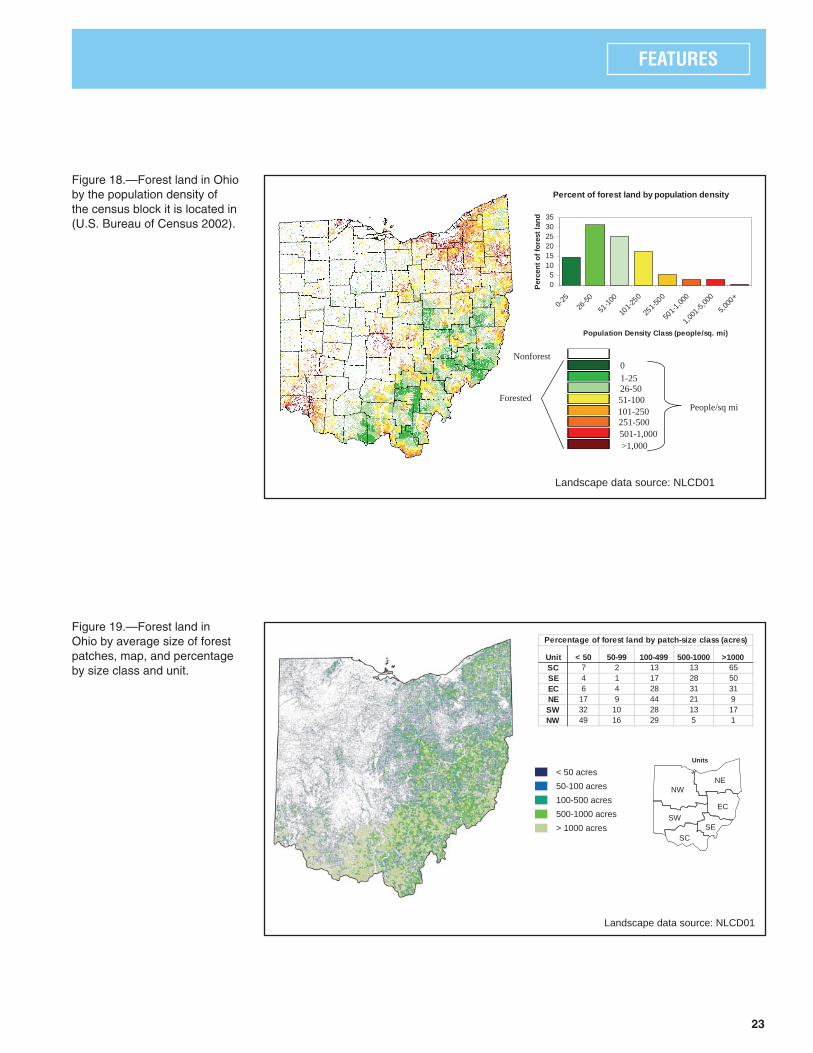
Changes in the numbers of trees have not been distributed evenly across diameter

classes (Fig. 27). Between 1968 and 1979, there were increases in the numbers of trees

across all diameter classes with large increases in the numbers of trees in the 6- and

8-inch diameter classes. The 1991 inventory showed a continuation of this trend with

increases across all diameter classes, although increases in the lower diameter classes

were less than previously. Since 1991, the number of trees has decreased in the 6- and

8-inch classes and the numbers of trees in the larger diameter classes have continued

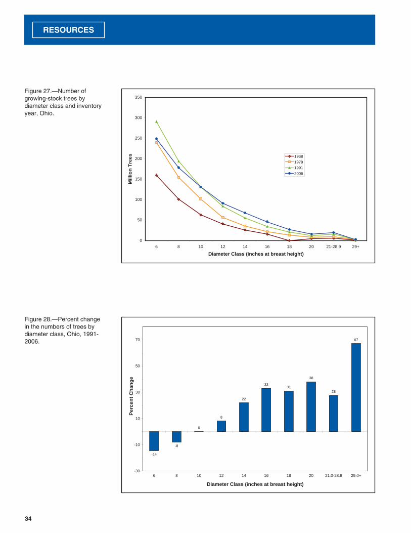
to increase. The curves of numbers of trees by diameter class have shifted to the right.

Generally, the larger the diameter class, the larger the percentage increase in numbers

of trees (Fig. 28).

Of trees 5 inches and larger in diameter, red maple is the most numerous species,

followed by sugar maple. Since 1979, numbers of these two species have increased by

109 and 92 percent, respectively. Between 1979 and 1991, white oak and aspen were

the only species to decrease in number, decreasing by 10 and 2 percent, respectively.

Since 1991, white oak has continued to decrease (-17 percent) and many more major

species are now showing decreases; additionally, hickory, beech, northern red oak, elm,

and chestnut oak have all decreased in numbers recently (Fig. 29). Major species to

show increases in numbers during the most recent inventory period were white pine,

yellow-poplar, aspen, and red and sugar maples.

Numbers of sapling-size trees (trees 1 to 4.9 inches in diameter) have decreased by

11 percent since 1991 in Ohio. Losses were spread among many major species with

large decreases in white ash, black cherry, elm, and all the oak species groups (Fig. 30).

There was also a large decrease in the numbers of noncommercial saplings. Beech is

notable in having a large increase in the number of sapling-size trees and a decrease

in the number of large beech trees. Of all the species, sugar maple saplings are most

numerous followed closely by those of red maple.

Numbers of Trees by Diameter Class

34

RESOURCES

Figure 28.—Percent change in the numbers of trees by diameter class, Ohio, 1991-2006.

-14

-8

0

8

22

3331

38

28

67

-30

-10

10

30

50

70

6 8 10 12 14 16 18 20 21.0-28.9 29.0+

Diameter Class (inches at breast height)

Perc

ent C

hang

e

Figure 27.—Number of growing-stock trees by diameter class and inventory year, Ohio.

0

50

100

150

200

250

300

350

6 8 10 12 14 16 18 20 21-28.9 29+

Diameter Class (inches at breast height)

Mill

ion

Tree

s 1968197919912006

35

RESOURCES

Figure 29.—Numbers of growing-stock trees 5 inches in d.b.h. and larger by species, Ohio, 1979, 1991, and 2006, and percent change 1991-2006.

0 20 40 60 80 100 120

Blackgum

Beech

White/red pine

Northern red oak

Chestnut oaks

Aspen

Black and scarlet oaks

White oak

White ash

Elm

Yellow-poplar

Black cherry

Hickory

Sugar maple

Red maple

Million Trees

197919912006

+1%

-12%

+24%

-13%

-16%

+5%

+1%

-17%

-26%

-34%

+10%

-1%

-10%

+23%

+14%

Figure 30.—Numbers of saplings (1 to 4.9 inches in d.b.h.) by species and percent change, Ohio, 1991 and 2006.

0 200 400 600 800 1,000 1,200

White pine

Chestnut oak

White oak

Aspen

Northern red oak

Black and scarlet oak

Blackgum

Beech

Yellow-poplar

Hickory

White ash

Black cherry

Elm

Red maple

Sugar maple

Noncomercial species*

Million Saplings

19912006

+8%

-18%

-27%

-4%

+26%

+14%

-1%

-37%

-29%

-35%

-3%

+10%

-34%

-7%

-20%

-41%

*Includes hawthorn, serviceberry, Osage-orange, American hornbeam, eastern hophornbeam, and other species with poor form.

36

RESOURCES

The numbers of large-diameter trees have increased steadily since 1968. The recent

decrease in 6- and 8-inch trees indicates that as trees grow into larger size classes

or succumb to competition they are not being completely replaced by smaller trees

growing into the lower classes. At the landscape level, Ohio’s forests have reached

the point where the total number of trees has begun to decline because of crowding.

Current trends indicate that the number of poletimber-size trees (5.0 to 10.9 inches

d.b.h. for hardwood species) will continue to decline as the number of large sawtimber-

size trees continues to increase.

Sapling-size trees represent the future forest. As large trees are harvested or succumb to

insects and diseases, they will be replaced by saplings now growing in the understory.

As this occurs the dominance of maple species in the understory will have an

increasing influence on the species composition of large-diameter trees. The decrease

in numbers of saplings is consistent with a maturing forest, which is especially true

for the decrease in noncommercial species that has occurred. Many noncommercial

species are pioneer species that need full sunlight to thrive.

What this means

Fully stocked sapling-size stand; photo by Richard Widmann, U.S. Forest Service

37

RESOURCES

Figure 31.—Percentage of growing-stock trees by crown position and diameter, Ohio, 2006.

The crown position of a tree indicates how well it is competing with neighboring

trees for light. A tree in an intermediate or overtopped crown position is below the

general level of the canopy and is shaded by its dominant and codominant neighbors.

Intermediate and overtopped trees generally can be expected to have slower growth

and higher mortality rates than trees in more dominant positions. The live crown

ratio or the percentage of a tree’s height in live crown is an indication of its vigor. Live

crown ratios of less than 20 percent are typically assumed to be a sign of poor vigor.

In the understory, trees with low live crown ratios have fallen behind in their struggle

with surrounding trees for light and space and are unlikely to ever recover or grow into

an overstory position.

In Ohio, most trees in the 2-, 4-, 6-, and 8-inch diameter classes are in an overtopped or

intermediate crown position—on average 86 percent (Fig. 31); conversely, 94 percent of

trees with diameters 14 inches or larger are either dominant or codominant.

Tree Condition—Crown Position and Live Crown Ratio

Background

What we found

0

10

20

30

40

50

60

70

80

90

100

2 4 6 8 10 12 14 16 18 20 21.0-28.9

29.0+

Diameter Class (inches at breast height)

Perc

ent o

f Tre

es in

Cla

ss

Overtopped and Intermediate trees

Codominant trees

Dominant trees

Open grown trees

38

RESOURCES

More than a third of trees in the 10-inch diameter class and below have live crown

ratios of less than 20 percent. For the 6-inch class, 40 percent have live crown ratios

below 20 percent (Fig. 32).

Shaded conditions created by overstory trees are stressing a large portion of trees

below 10 inches in diameter. This finding is consistent with the maturing of Ohio’s

forests and the likely cause for decreases in numbers of trees in the 6- and 8-inch

diameter classes. Shaded conditions favor the growth of shade-tolerant species such as

sugar maple over that of less shade-tolerant species such as American elm, white ash,

and the oaks.

Figure 32.—Percentage of growing-stock trees with a live crown ratio of 20 percent or less by diameter, Ohio, 2006.

What this means

0

10

20

30

40

2 4 6 8 10 12 14 16 18 20 21.0-28.9

29.0+

Diameter Class (inches at breast height)

Perc

ent o

f Tre

es in

Cla

ss

Live crown ratio less than 20 %

39

RESOURCES

Background The species composition of a forest

is the result of the interaction

of climate, soils, disturbance,

competition among trees species,

and other factors over time.

Causes of forest disturbance in

Ohio include wildfires, ice storms,

logging, droughts, insects and

diseases (e.g., Dutch elm disease),

and land clearing followed by

abandonment. Also, as forests

mature, changes in growing

conditions favor the growth of

shade-tolerant species. Forest

attributes that describe forest

composition include forest type,

forest-type group, numbers of trees

by species and size, and changes in

the species makeup of total volume.

Forest types describe groups of species that frequently grow in association with one

another and dominate the stand. Similar forest types are combined into forest-type

groups. While large trees represent today’s forest, the composition of the lower

diameter classes represents the future forest. Comparisons of species composition by

size can provide insights into future overstory changes.

The 2006 inventory of Ohio identified 109 tree species, 48 forest types, and 11

forest-type groups. The oak/hickory group covers more than half (4.1 million acres)

of Ohio’s forests, and the northern hardwood group covers another third (2.4 million

acres) (Fig. 33). The oak/hickory group consists of white oak, northern red oak,

hickory species, white ash, walnut, yellow-poplar, and red maple. Eighty-five percent of

oak volume and 64 percent of red maple volume in the State grow in the oak/hickory

group, while 78 percent of sugar maple volume and 60 percent of beech volume grow

in the northern hardwood group. These broad species groups have changed little in

area since 1991.

Sugar maple is the most numerous sapling (1 to 4.9 inches d.b.h.) followed by

red maple (Fig. 34). Among trees between 5 and 10.9 inches d.b.h., red maple is

most numerous followed by sugar maple. Together the oaks are most numerous in

Forest Composition

What we found

Sawtimber-size stand of white oak; photo by Richard Widmann, U.S. Forest Service

40

RESOURCES

Figure 34.—Number of trees for selected species by diameter class, Ohio, 2006.

0

50

100

150

200

6 8 10 12 14 16 18 20 21-28.9

29+

Diameter Class (inches at breast height)

Beech

Hickory

Sugar maple

Red maple

Oaks

0

100

200

300

400

500

600

700

800

900

2 4

Mill

ion

Tree

s

Figure 33.—Area of timberland by forest-type group, Ohio, 2006 (error bars represent 67-percent confi dence intervals around the estimates).

0 0.5 1 1.5 2 2.5 3 3.5 4 4.5 5

Oak/gum/cypress

Exotic softwoods

Pinyon/juniper

Loblolly/shortleaf

White/red pine

Aspen/birch

Oak/pine

Elm/ash/red maple

Northern hardwoods

Oak/hickory

Million Acres

1991

2006

41

RESOURCES

diameter classes 11 inches and larger. In the current inventory, oaks represent more

than one-third of the trees 20 inches and larger in diameter, but only 5 percent of

trees in the 2- and 4- inch diameter classes (Fig. 35). Conversely, maple species have

a disproportionate share of trees in the 2- and 4-inch diameter classes—27 percent—

compared to their presence in the larger diameter classes—14 percent of trees 20 inches

d.b.h. and larger. Elm also has a disproportionately large share of trees in the 2- and

4- inch diameter classes—8 and 25 percent, respectively. Oaks have been decreasing as a

percentage of total growing-stock volume since 1968, while maple species have had an

increasing share of total volume since 1952 (Fig. 36).

The small shift in area from the oak/hickory forest-type group to other groups does

not fully depict the underlying shifts going on in individual species. A lack of oaks in

the small diameter classes means that as large oaks are harvested or die, they will likely

be replaced by species such as red and sugar maples that dominate the lower diameter

classes. Maples will play an increasing role in Ohio’s future forest. The area occupied

by the oak/hickory forest-type group is likely to undergo a long-term decline and be

replaced by the northern hardwood group.

Decreases in the oak proportion of the resource have been attributed to inadequate

oak regeneration and the subsequent lack of oak growing into larger diameter classes,

and selective harvesting of oak over other species. Generally, current forest practices

do not promote the regeneration of oaks, and silvicultural tools to promote oak

are not being used. Contributing factors to poor oak regeneration are lack of fire,

understory growing conditions that favor more shade-tolerant hardwoods, white-tailed

deer preferentially browsing oak seedlings, and smaller openings from low intensity

harvesting. Long-term changes in forest composition can alter wildlife habitats and

affect the value of the forest for timber products.

What this means

42

RESOURCES

Figure 35.—Species composition by diameter class, Ohio, 2006.

Figure 36.—Change in selected tree species as a percentage of total growing-stock volume, Ohio, 1952-2006.

0

25

50

75

100

2 4 6 8 10 12 14 16 18 20 21-28.9 29+

Diameter Class (inches at breast height)

Indi

vidu

al S

peci

es a

s a

Perc

enta

ge o

f To

tal N

umbe

r of T

rees

in C

lass

OaksRed maple

Sugar maple

Hickory

W. ashB.cherry

Y. poplar

Noncommercial

All other species

BeechElm

0

10

20

30

40

60021991979186912591

Inventory Year

Perc

ent o

f Vol

ume

in C

lass

All oaks Maple species Hickory Elm Y.-poplar

43

RESOURCES

Background Displaying the distribution of individual species spatially shows where a species is

concentrated and where it is sparse. Species are distributed by how well they are

suited to particular site conditions and by the frequency of disturbances such as

wildfire, timber harvesting, insect and disease outbreaks, and land clearing followed

by reforestation. At the landscape scale, broad geophysical and biophysical features are

apparent such as the extent of glaciers, and land use patterns.

FIA has mapped species distributions by taking the percentage of total basal area

represented by each species on inventory plots and using it to make estimates of forest

composition across the landscape. The highest category represents areas where a single

species represents more than half the stocking of live trees. In the middle category, the

mapped species represents a substantial portion (10 to 50 percent of stocking) of the

stand. And in the lowest category, the mapped species is not present or is scattered.

The major species of trees growing in Ohio are well distributed throughout the State.

An example of this is red maple, a component of nearly every forest type in the State

(Fig. 37). Red maple is concentrated mostly in the Northeastern Unit where soils tend

to be poorly drained. Here red maple has seeded on abandoned farm land. Sugar

maple also grows on a wide range of site conditions but typically does better on well-

drained soils than on swampy or thin dry soils (Richard M. Godman et al. 1990). Sugar

maple is commercially important chiefly in northeastern Ohio where it is associated

with beech. Hickory grows throughout Ohio, but infrequently represents more than

half the stand basal area. Yellow-poplar grows most abundantly on the west side of the

Appalachian Mountains, where it grows well on lower slopes and sheltered coves. In

Ohio it reaches its greatest abundance in the southeastern portion of the State. Black

cherry is abundant in northeast Ohio but nearly absent from the southernmost part of

the State. White ash is widely distributed. Its highest concentrations are in the center

of the State where it frequently represents more than half the stocking. Together the

oaks generally grow more abundantly in the unglaciated southeastern portion of the

State. Here they are more tolerant to dry conditions in the thin upland soils than some

of the other major species. This is especially true for chestnut oak, which grows mainly

on dry ridges. Historically, wildfires have also promoted the growth of the oaks over

other species in southern Ohio.

Across the State, there are few areas where any one species represents more than half

the stocking of live trees. Each of the 10 major species typically represents between 10

and 50 percent of stocking where it occurs. Ohio’s diverse mix of species reduces the

impact of insects and disease that target a single tree species.

Distribution of Common Species

What we found

What this means

44

RESOURCES

Figure 37.—Distribution of common tree species, Ohio, 2006.

Percent of total live basal area

<10

10 - 50

>50

Nonforest /not measured

Percent of total live basal area

<10

10 - 50

>50

Nonforest /not measured

Red maple Sugar maple

American beech Hickory

Yellow-poplar

45

RESOURCES

Percent of total live basal area

<10

10 - 50

>50

Nonforest /not measured

Percent of total live basal area

<10

10 - 50

>50

Nonforest /not measured

Black cherry

Northern red oak Chestnut oak

White oak

White ash

Figure 37.—continued.

46

RESOURCES

Figure 38.—Components of total volume, Ohio, 2006.

Measurement of growing-stock volume on timberland is important in assessing

the volume of wood available for commercial products. Trees in this category meet

minimum requirements for size and straightness, are within tolerances for rot, and are

of commercial species. These trees are considered crop trees in silvicultural treatments

where the goal is to maximize economic returns. Growing-stock volume is the resource

base on which the forest products industry depends. Measures of growing-stock volume

are useful in making comparisons to older inventories where only estimates of growing

stock are available.

Ninety-two percent of the sound wood volume in live trees is contained in growing-

stock trees, which are commercially important species with good form. Rough and

rotten trees account for 7 and 1 percent, respectively (Fig. 38). The total volume of

growing stock on Ohio’s timberland has steadily increased since 1968. The 2006

estimate of 12.3 billion cubic feet is 22 percent more than in 1991 and averages

1,603 cubic feet per acre (Fig. 39, 40). Forest inventories show a steady shift in timber

volume toward larger trees (Fig. 41). During the most recent inventory period, volume

increased in all classes greater than 8 inches, but the volume of trees decreased in the

6- and 8-inch diameter classes (Fig. 42). Most of the gains in volume were in trees large

Background

What we found

Growing-stock trees 12.3 billion cubic feet

92%

Rough trees1.0 billion cubic feet

7%

Rotten trees 0.1 billion cubic feet

1%

Volume of Growing-stock Trees

47

RESOURCES

Figure 39.—Growing-stock volume by inventory year, Ohio, 1968, 1979, 1991, and 2006 (error bars represent 67-percent confi dence intervals around the estimates).

Figure 40.—Average growing-stock volume (board feet and cubic feet) per acre of timberland, Ohio, 1968, 1979, 1991, and 2006.

Figure 41.—Growing-stock volume by diameter class and inventory year, Ohio, 1961, 1975, 1989, and 2006 (error bars represent 67-percent confi dence intervals around the estimates).

Figure 42.—Percent change in volume by diameter class on timberland, Ohio, 1979-1991 and 1991-2006.

12.3

10.0

6.4

4.2

0

2

4

6

8

10

12

14

1968 1979 1991 2006

Inventory Year

Bill

ion

Cub

ic F

eet

661

924

1,603

1,319

5,338

2,299

2,952

3,979

0

500

1,000

1,500

2,000

1968 1979 1991 2006

Cub

ic Fe

et/A

cre

0

1,000

2,000

3,000

4,000

5,000

6,000

7,000

Inventory Year

Boa

rd F

eet/A

cre

Cubic feet Board feet

0

500

1,000

1,500

2,000

6 8 10 12 14 16 18 20

Diameter Class (inches at breast height)

Mill

ion

Cub

ic F

eet

1968 1979 1991 2006

Poletimber size Sawtimber size

4339

46

66

75 7469

57

4

16

30

4440

50

-6-10

-20

0

20

40

60

80

100

6 8 10 12 14 16 18 20

Diameter Class (inches at breast height)

Perc

ent C

hang

e

1979-1991 1991-2006

48

RESOURCES

enough to produce saw logs (11.0 inches in d.b.h. and greater for hardwood species),

which reflects the changes in the numbers of trees discussed previously. The portion of

volume large enough to produce saw logs increased by 35 percent to 41 billion board

feet. Although recent gains are a continuation of increases that have been occurring

over the last 40 years, the rate of increase is slowing. During the previous inventory

period, 1979 to 1991, gains in growing-stock and sawtimber volumes were larger than

in 1991 to 2006; 57 and 48 percent, respectively.

Yellow-poplar continues to lead in volume followed by red maple and sugar maple.

These three species also had the largest volume gains since 1991(Fig. 43). All of the

oak species groups had increases in volume although these increases were generally less

than many of the other major species. Together oak species increased in volume by 13

percent versus 22 percent for total volume. Of the major species, only white ash, elm,

and American beech showed decreases in volume since the previous inventory.

In board-foot volume, the top ranked species differ little from those for all growing-

stock volume (Fig. 44). Yellow-poplar remains the leading species, accounting for 12

percent of total board-foot volume followed by white oak and hickory. Together the

oaks represent 27 percent of total board-foot volume and maples 15 percent. Ninety-six

percent of Ohio’s sawtimber volume is in hardwood species.

Average volumes per acre are highest in Ohio’s Southeastern Unit (Fig. 45). This

unit also has had a large increase in volume per acre since the previous inventory—37

percent. The Southeastern Unit includes much of the Wayne National Forest, which

has high volumes per acre, averaging 1,935 cubic feet of growing stock per acre. The

East-Central Unit has the lowest volumes per acre and the smallest percentage increase

in volume per acre. In the Northwestern Unit, volumes per acre were comparable to

the rest of the State, although this region had the lowest increase in total volume.

Yellow-poplar is the leading species in the three unglaciated units (East-Central,

Southeastern, and South-Central) (Fig. 46). These units account for 89 percent of the

State’s yellow-poplar volume. White ash is the leading species in the Northwestern and

Southwestern Units where it accounts for 15 percent of the total volume in each unit.

Red maple, the leader in the Northeastern Unit, has nearly doubled in volume since

the previous inventory and now makes up 20 percent of the volume in the unit.

49

RESOURCES

Figure 43.—Growing-stock volume on timberland by species and percent change, Ohio, 1991 and 2006 (error bars represent 67-percent confi dence intervals around the estimates).

Figure 44.—Board-foot volume on timberland by species and percent change, Ohio, 1991 and 2006 (error bars represent 67-percent confi dence intervals around the estimates).

0 500 1,000 1,500

Blackgum

Basswood

Beech

Elm

Aspen

Chestnut oak

Softwoods

Northern red oak

White ash

Black and scarlet oak

Black cherry

White oak

Hickory

Sugar maple

Red maple

Yellow-poplar

Million Cubic Feet

19912006

+25%

+11%

-7%

-22%

+59%

+15%

+47%

+16%

+33%

+43%

+45%

+20%

+15%

+9%

-3%

+12

0 1 2 3 4 5 6

Blackgum

Basswood

Elm

Beech

Aspen

Softwoods

Chestnut oak

Black cherry

White ash

Northern red oak

Black and scarlet oak

Sugar maple

Red maple

Hickory

White oak

Yellow-poplar

Billion Board Feet

19912006

+62%

+16%

+33%

+16%

+57%

+35%

+38%

+36%

+23%

+25%

+24%

+13%

+67%

+73%

+6%

+28%

50

RESOURCES

Figure 45.—Average cubic-foot and board-foot volumes per acre of timberland by unit, 2006, and percent change, Ohio, 1991-2006.

Figure 46.—Top fi ve species by unit and percent change by volume, Ohio, 1991-2006.

Northwestern1,731 CF/ac +17% Northeastern

East-Central

Southwestern

Southeastern

South-Central

State1,603 CF/ac +22% 5,338 BF/ac +34%

5,893 BF/ac +34%1,580 CF/ac +10%5,122 BF/ac +28%

1,631 CF/ac +33%5,122 BF/ac +28%

1,847 CF/ac +37%6,278 BF/ac +47%

1,375 CF/ac +9%6,278 BF/ac +47%

1,595 CF/ac +37%5,338 BF/ac +39%

Red maple +91% Black cherry +9%Sugar maple +6%Hickory +34%Black/scarlet oaks +48%

Northeastern

South-Central

Southeastern

East-Central

Southwestern

Northwestern

Yellow-poplar +5%Black cherry +49%Red maple +12%Sugar maple +19%Hickory +12%

Yellow-poplar +76%White oak +31%Sugar maple +65%Red maple +70%Hickory +50%

Yellow-poplar +92%White oak -6%Hickory +25%Sugar maple +36%Chestnut oak +46%

White ash +21%Sugar maple +19%Hickory +3%Black cherry +57% Northern red oak +72%

White ash +15%Hickory -20%Sugar maple -2%Red maple -6%Black/scarlet oaks +12%

51

RESOURCES

What this means Continuous increases in volume have brought Ohio’s timber resource to record

levels in both total growing-stock volume and volumes per acre. And most trees

meet minimum requirements to qualify as growing-stock trees. Timber growth is

concentrated on sawtimber-size trees (more than 11 inches in d.b.h.), which explains

why increases in board-foot volume (+35 percent) were more than those in cubic-foot

volume (+22 percent). As trees grow in sawtimber size, their value for timber products

jumps because they can now be used for higher value products. Because more growth

is being put on higher value trees than previously, Ohio’s forests are now adding value

at an increasing rate, although rates of volume increase are slowing. This increase in

value is good for landowners and the forest products industry. But, as the number of

new trees growing into sawtimber size decreases, as shown by decreases in the numbers

of 6- and 8-inch trees, harvesting practices become an increasing concern. Any

mismanagement of sawtimber stands, if it occurs, will become more apparent in stands

where most growth is occurring on residual sawtimber-size trees left after harvesting

operations.

Changes in volume by species reflect changes that are occurring in species composition.

Volume increases for the maples are larger than those for the oaks, although all oak

species increased in volume. Oaks are doing better in Ohio than in the surrounding

states of Pennsylvania, West Virginia, and Indiana, where many of the oak species have

shown smaller increases or decreases in volume.

In the Northwestern Unit, increases in average volume per acre were comparable to the

rest of the State, but total growing-stock volume increased by only 3 percent because

of the loss of forest land. Decreases in volume of some of the leading species in this

unit were also probably caused by loss of forest land. Because white ash is the leading

species in the Northwestern and Southwestern Units, future mortality caused by the

emerald ash borer will likely be significant in these areas. In the Northeastern Unit, red

maple has proliferated on abandoned farm land. Because most red maple volume is in

poletimber or small sawtimber-size trees, large increases in red maple volume are likely

to continue there.

The East-Central Unit has lower volumes per acre and has had a smaller increase in

volume since the previous inventory than the rest of the State. This finding is probably

due to the region’s land use history; large areas of forest in this unit are reclaimed strip

mines with generally poor soils.

52

RESOURCES

The use of the timber resource for sawn timber products is determined largely by

tree quality and species. The best trees are used in the manufacture of furniture,

cabinets, and other millwork that command high prices. Lower quality trees are used

for pallets, pulpwood, and fuelwood. Quality varies by species due to differences in

average diameter, growth characteristics, and past management practices. FIA assigns

tree grades to sawtimber-size trees as a measure of quality. Tree grades are based on

the amount of knot-free bole, amount of cull, and tree diameter. Trees need to be at

least 13 inches d.b.h. to be considered for a grade 2, and 16 inches d.b.h. for a grade 1.

Grade 1 yields the most high-grade lumber and tie/local use grades the least.

The portion of sawtimber volume in tree grades 1 and 2 increased from 32 percent of

total sawtimber volume in 1991 to 43 percent in 2006 (Fig. 47). In absolute terms the

volume in grades 1 and 2 increased from 9.2 billion board feet in 1991 to 17.1 billion

in 2006. Volume in the lowest grade (tie/local use) increased from 8.0 to 10.3 billion

board feet, although it decreased as a portion of total volume to 26 percent.

In Ohio, yellow-poplar has the largest volume in tree grades 1 and 2, followed by white

ash, northern red oak, basswood, and white oak (Fig. 48). These species, as well as

chestnut oak and blackgum, have at least half of their sawtimber volume in tree grade

2 or better. Of the other major species in the State, beech had the lowest portion of

volume in grades 1 and 2, followed by red maple, sugar maple, and black cherry. Many

beech trees in Ohio are degraded because of large amounts of rotten wood. Red maple

Variation in Hardwood Quality by Species

Background

What we found

Figure 47.—Hardwood board-foot volume by tree grade, Ohio, 1991 and 2006.

0

10

20

30

40

50

60021991Inventory Year

Bill

ion

Boa

rd F

eet

Grade 1Grade 2Grade 3Tie/local use

11%

21%

41%

27%

24%

30%

26%

19%

53

RESOURCES

is graded lower than other species because it typically has more defects and smaller

diameters. Beech, red maple, and sugar maple also do not self prune as well as other

species such as yellow-poplar and white ash.

Because small sawtimber-size trees are assigned a low grade on the basis of size alone,

the increase in size of Ohio’s trees has brought about an increase in saw log quality.

Combined with increases in saw log volume, this represents a tremendous increase in the

value of the forest resource for timber products. This increase is best shown by looking at

yellow-poplar, which leads the State in board-foot volume; it had the largest increase in

board-foot volume (62 percent) of all species between 1991 and 2006 and has the highest

portion of its volume in grade 2 or better trees (64 percent). Countering the increase in

quality because of tree size are changes in species composition. Red and sugar maples

had some of the largest increases in volume but typically grade poorer than other major

species. Future tree quality may be affected by changes in species composition.

In Ohio, about one-third of hardwood sawtimber volume is in trees less than 15 inches

in d.b.h. These trees are too small to be rated grade 1. Forest land owners can receive

high financial returns by practicing best management practices and favoring trees

with the potential to grow into higher quality grade 1 and 2 trees. This rewards the

landowner and greatly benefits the State’s wood-using industries through value added

in manufacturing.

Figure 48.—Percentage of saw log volume by tree grade for major species, Ohio, 2006.

7

9

11

12

14

17

17

22

26

30

31

32

34

8

13

21

23

27

13

34

19

30

35

31

33

28

30

21

32

40

43

37

41

34

33

23

27

25

30

18

28

23

71

49

30

26

29

20

39

16

40

21

15

10

18

13

12

9 22

0 10 20 30 40 50 60 70 80 90 100

Beech

Red maple

Sugar maple

Elm

Black cherry

Hickory

Aspen

Blackgum

Other red oaks

Chestnut oak

White oak

Basswood

Northern red oak

White ash

Yellow-poplar

Percent of VolumeGrade 1 Grade 2 Grade 3 Tie/local use

What this means

54

RESOURCES

Trees play an important role in the world’s carbon cycle. They act as a sink for carbon,

removing it from the atmosphere in the form of carbon dioxide (a greenhouse gas)

and storing it as cellulose. In this role, forests help mitigate the effect of burning fossil

fuels and the resulting global climate change associated with increased levels of carbon

dioxide in the atmosphere. Ohio’s forests contribute greatly to the sequestration of

carbon dioxide due to increases in tree volume.

Tree biomass, a measure of how much carbon is being stored on forest land, is the

total weight of both live and dead trees, including branches, roots, and stumps.

Biomass of all trees standing in Ohio’s forests equals 635.2 million dry tons—an

average of 80 tons per acre. The greatest portion (54 percent) is in the merchantable

boles of commercially important trees (Fig. 49). It is this component that can be

converted to high-value wood products. Other portions of biomass are underutilized

and can be considered as a potential source of fuel for commercial power generation.

Biomass in trees 5 inches and larger in diameter has increased by 20 percent since

1991. The greatest concentrations of biomass in Ohio are in the Southeastern and

South-Central Units (Fig. 50).

Biomass Volume of Live Trees

Background

What we found

Understory shrubs benefi t wildlife; photo by Richard Widmann, U.S. Forest Service

55

RESOURCES

Figure 49.—Components of tree biomass on forest land in Ohio, 2006.

Figure 50.—Biomass of standing trees by county, Ohio, 2006.

Ohio BiomassDry Tons (Millions)

< 8.0

8.0 - 11.9

12.0 - 15.9

16.0 - 19.9

20.0 +

Growing stock54%

Branches/foliage

9%

Stumps/roots18%

Cull trees12%

Saplings/seedlings

6%

Dead trees1%

Total tree biomass= 635,223,000 dry tons

56

RESOURCES

Ohio’s forests are accumulating substantial amounts of biomass. These stores of carbon

will receive increasing attention as the Nation seeks sources for renewable energy

and ways to offset carbon dioxide emissions. Because biomass is a renewable source

of energy, it can help reduce the Nation’s dependence on fossil fuels and provide

markets for low-grade wood. Any new plant that turns woody biomass to energy would

need a large local source of biomass to keep transportation costs low. The higher

concentrations of biomass in southeastern Ohio would make the region the most likely

location for such a plant.

Forest landowners are not financially compensated for contributions their trees make

in absorbing carbon dioxide and storing carbon. However, this may change if recent

proposals to pay landowners for storing carbon in their forests become a widespread

reality. The Chicago Climate Exchange has recently developed a financial instrument

to trade carbon contracts for forest carbon sequestration to offset emissions of

greenhouse gases. Improvements in how biomass is measured and accounted for would

likely help promote this new income source for landowners.

What this means

Debris left after harvesting is a potential source for biomass fuel; photo by Richard Widmann, U.S. Forest Service

57

RESOURCES

Background

What we found

Figure 51.—Annual components of change in growing-stock volume, Ohio, 1991-2006.

Well-tended forests supply a continuous flow of products without impairing long-

term productivity. Unlike coal and oil, forests are alive and renewable. One way to

judge the sustainability of a forest is to look at the components of annual change in

inventory volume—growth, removals, and mortality. Removals include trees harvested

on land that remains in timberland, trees on timberland that has been reclassified to

reserved forest land, and trees lost because the forest was developed for a nonforest

use. Analysis of these individual components can help us better understand what is

influencing net change.

During the last 50 years in Ohio, the growth of trees has greatly outpaced mortality

and removals. The most recent inventory revealed that since 1991, on an annual

basis, gross growth has totaled 419 million cubic feet (Fig. 51). Eighty-one percent

of this growth was accretion (growth on trees that were at least 5 inches in diameter

at the time of the previous inventory) and 19 percent was ingrowth (trees less than

5 inches in diameter that grew to at least 5 inches in diameter). Annual mortality

averages 99 million cubic feet, resulting in a net growth of 320 million cubic feet. The

removals of trees due to both harvesting and land use change averaged 160 million

cubic feet, leaving an annual surplus or net change of 160 million cubic feet on Ohio’s

timberland. About two-thirds of the removals was due to the harvesting of trees and

Components of Annual Volume Change

81

338

419

320

-160

160

-99

-300

-100

100

300

500

Ingrowth Accretion Gross growth Mortality Net growth Removals Net change

Components of Change

Mill

ion

Cub

ic F

eet

65% due to harvesting 32% due to land use changed to nonforest use 3% due to land use changed to reserved forest land

58

RESOURCES

Figure 52.—Average annual net growth, removals, and growth-to-removals (G/R) ratio for major species, Ohio, 1991-2006.

What this means

the remainder was due to changes in land use. As a percentage of the inventory, gross

growth was 3.8 percent, mortality—0.9 percent, net growth—2.9 percent, removals—1.4

percent, and net change—1.4 percent.

The net change of 160 million cubic feet was nearly the same as during the 1979-1991

inventory period, although all the components were greater. Greater growth was offset

by increases in both mortality and removals.

The ratio of growth-to-removals (G/R) averaged 2.0:1 for 1991-2006, but varied

considerably between species (Fig. 52). Net growth exceeded removals for all major

species except elm, which had negative growth due to high mortality. Yellow-poplar

had the largest amount of removals, but its growth still exceeded removals by 2.6 to

1. Northern red oak and white oak ranked second and third in removals, respectively.

Their removals nearly matched their growth with growth-to-removals ratios of 1.0:1

and 1.1:1, respectively. Red maple had the largest amount of growth, with growth

exceeding removals by 4.1:1.

Today’s well-stocked forests are a product of growth consistently outpacing removals

during the last half century and the surplus accumulating in the forest. Since 1991 net

growth has been twice that of removals; the net change has amounted to an annual

increase of 1.4 percent in inventory volume. This finding implies that the current level

-5 5 15 25 35 45 55

Elm

Blackgum

Beech

Basswood

Aspen

Northern red oak

White oak

Chestnut oak

Black and scarlet oak

Softwoods

Black cherry

Hickory

White ash

Sugar maple

Yellow-poplar

Red maple

Million Cubic Feet

Net growthTotal removals

4.1 : 1

2.6 : 1

2.8 : 1

2.1 : 1

1.8 : 1

2.9:1

1.6:1

1.5:1

19.8:1

-0.6:1

1.4:1

7.2:1

2.4:1

1.0:1

1.1:1

1.6:1

G/R all species = 2.0 :1

59

RESOURCES

of removals is sustainable and that increases in timber volumes will continue. For the

most part, this is true: nearly two-thirds of removals are due to harvesting and trees

regenerate and thrive after harvesting as long as the land remains in forest. And the

small portion of removals due to timberland being reclassified to reserved forest land

will continue to provide benefits other than timber products. But, the nearly third of

removals due to conversion of timberland to nonforest uses threatens sustainability

because such changes usually are permanent. As a result, future timber growth from

these lands is lost, as are related benefits, such as the recharge of groundwater aquifers

and forest habitats.

A characteristic of a maturing forest is the growth shift from ingrowth to accretion.

In 2006, four-fifths of growth in Ohio was accretion on trees larger than 5 inches

d.b.h. and the remaining fifth was from trees growing into 5-inch or larger diameter

classes. This means that small trees will have a diminishing effect on changes in species

composition, because it is more likely that existing trees will fill in gaps created by

mortality and harvesting rather than ingrowth of small trees.

Comparing the growth-to-removals ratios of individual species to the average ratio for

all species (2.0:1) reveals which species are increasing in importance and which are

decreasing. The high growth-to-removals ratios for red maple, sugar maple, and yellow-

poplar show these species will increase in importance in Ohio’s forests. These ratios

help us better understand shifts in species composition, particularly when comparing

species with high ratios such as the maples to those with relatively low ratios such as

many of the oaks.

Large sapling stand; photo by Richard Widmann, U.S. Forest Service

60

RESOURCES

The volume of trees that die from natural causes such as insects, diseases, fire, wind,

and suppression from other trees is reported as mortality; harvested trees are not

included. Tree mortality is a natural process that occurs in a functioning ecosystem

although dramatic increases in mortality can indicate problems in forest health.

In Ohio, average annual mortality was 99 million cubic feet, a rate of 0.9 percent of

inventory volume. This is an increase from the previous inventory (1979-1991) when

annual mortality averaged 57 million cubic feet or 0.6 percent. Despite this increase,

Ohio’s mortality rate is similar to neighboring states and is considered normal:

Michigan 0.8, West Virginia 0.9, Pennsylvania 0.9, and Indiana 0.9. Mortality rates

were higher for smaller diameter trees than for larger ones (Fig. 53). The mortality rate

in the 6-inch class was 1.9 percent per year, which is more than twice the average rate

across all diameter classes. The 16-inch class had the lowest mortality rate—0.5 percent.

Trees less than 11 inches in diameter accounted for 40 percent of total mortality, even

though most mortality occurred in sawtimber-size stands (76 percent).

Species groups with high annual mortality rates were elm, aspen, and softwoods—4.1,

1.6, and 1.4 percent, respectively (Fig. 54). Five of the major species groups account for

more than half the total mortality: elm (19 percent), white ash (10), hickory (8), black

cherry (8), and softwoods (7).

Mortality

Background

Figure 53.—Average annual mortality rate (in percent) of growing-stock volume on timberland by diameter class, Ohio, 1991-2006.

What we found

1.9

1.3

0.80.9 0.8

0.50.6

1.0

0.8

0.9

0.0

0.5

1.0

1.5

2.0

2.5

6 8 10 12 14 16 18 20 21-28.9 29+

Diameter Class (inches at breast height)

Average for all class = 0.9%

61

RESOURCES

Tree mortality rates in Ohio have increased since previous inventories, although they are

still comparable to those in surrounding states. Much of the mortality can be explained

by stand dynamics and insects and diseases that target specific species. The maturing of

Ohio’s forests has resulted in more crowded growing conditions. As trees compete for

light and growing space, some fall behind their neighbors, lose vigor, and eventually

succumb to insects and diseases. This is evident in the condition of small trees. As

discussed earlier, most trees less than 8 inches in diameter grow in the understory (Fig.

31), and a third of trees less than 10 inches in diameter have live crowns less than 20

percent of their height—a sign of poor vigor in the lower diameter classes (Fig. 32).

Even though most species have low mortality rates, some are not so fortunate. These

species have increased the overall mortality rate for the State. The high rate of

mortality for elm can be attributed to Dutch elm disease. Some of the ash mortality can

probably be attributed to the emerald ash borer that has been found in northwestern

Ohio, although other diseases also attack ash. Ash decline and ash yellows have been

ongoing problems for ash. Other species groups with high mortality rates are aspen, all

softwoods, and black cherry, which are mostly early succession species that are intolerant

to shade. Pitch and Virginia pine are responsible for most of the mortality in the

softwood group. These two species likely became established when wildfires were much

more prevalent than they are today and are slowly being replaced by hardwood species in

Ohio, as well as in many neighboring states, as natural succession progresses.

Figure 54.—Average annual mortality rate (in percent) for major species, Ohio, 1991-2006.

What this means

0.4

0.4

0.5

0.5

0.5

0.5

0.7

0.8

0.9

1.0

1.0

1.1

1.3

1.4

1.6

4.1

0.0 0.5 1.0 1.5 2.0 2.5 3.0 3.5 4.0 4.5

Elm

Aspen

All softwoods

White ash

Black cherry

Northern red oak

Beech

Basswood

Hickory

Black/scarlet oak

Chestnut oak

White oak

Blackgum

Sugar maple

Yellow-poplar

Red maple

Average Annual Mortality Rate (percent)

Average for all species = 0.9%

62

RESOURCES

Background

What we found

Figure 55.—Number of oak trees by diameter class, Ohio, 1991 and 2006.

Concern is growing about the sustainability of oaks across the oak/hickory forests

of the Northern States. Oak species serve as keystone species in the forest ecosystem

in that they create a community structure and environment that maintains critical

ecosystem processes (Fralish 2004). The hard mast oaks provide is especially important

because of the demise of American chestnut (Castanea dentate) and reduced numbers

of large American beech (Fagus grandifolia) in many areas because of beech bark disease.

Oaks are also important to the forest products industry.

Analysis of inventory data typically looks at changes in growing-stock volume. In Ohio

the cubic-foot volume of oaks increased by 13 percent and board-foot volume increased

by 21 percent between the 1991 and 2006 inventories. Because volume estimates are

heavily influenced by changes in large trees, further examination of the numbers of

trees, especially in the lower diameter classes, can give us insight into future changes in

oaks.

Ohio has had an overall decrease in the numbers of small trees. Decreases in small

trees are more pronounced in oaks than in non-oak species (Figs. 55, 56). By 2-inch

diameter class, numbers of oaks have decreased in the 2-, 4-, 6-, 8-, 10-, and 12-inch

classes since 1991, whereas all non-oak species decreased in only the 2- and 4-inch

classes. The oak portion of trees declined in most diameter classes between the 1991

and 2006 inventories, with large decreases in diameter classes 8 through 12 inches (Fig.

57). Only in the 29-inch and larger diameter class did the portion of oaks increase.

Oaks are well represented in the large diameter classes but are poorly represented in

Status of Oaks

0

5

10

15

20

25

30

35

6 8 10 12 14 16 18 20 21-28.9

29+

Diameter Class (inches at breast height)

1991 2006

020406080

100120140160

2 4

Mill

ion

Tree

s

63

RESOURCES

Figure 56.—Comparison of oaks and all other non-oak species as a percentage of total trees by diameter in class, Ohio, 2006.

Figure 57.—Oaks as a percentage of total number of trees in class, 1991 and 2006.

-41

-6

-22-25

-16

7 914

31 34

77

0

8

1922

32

48 46 49

34

58

-19 -17 -20

-60

-40

-20

0

20

40

60

80

100

2 4 6 8 10 12 14 16 18 20 21-28.9 29+

Diameter Class (inches at breast height)

Perc

ent C

hang

e in

Num

bers

of

Tre

es in

Cla

ss

All oaks All non-oak species

57

8

12

16

20

23

3132

36 36

46

5 5

89

11

14

19

25

27

33

36

49

0

10

20

30

40

50

2 4 6 8 10 12 14 16 18 20 21-28.9 29.0+

Diameter Class (inches at breast height)

Perc

ent o

f Tre

es in

Cla

ss

1991 2006

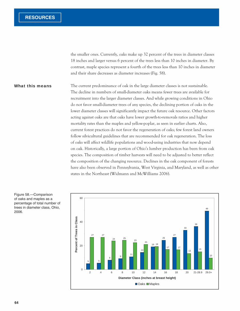
64

RESOURCES

What this means

Figure 58.—Comparison of oaks and maples as a percentage of total number of trees in diameter class, Ohio, 2006.

the smaller ones. Currently, oaks make up 32 percent of the trees in diameter classes

18 inches and larger versus 6 percent of the trees less than 10 inches in diameter. By

contrast, maple species represent a fourth of the trees less than 10 inches in diameter

and their share decreases as diameter increases (Fig. 58).

The current predominance of oak in the large diameter classes is not sustainable.

The decline in numbers of small-diameter oaks means fewer trees are available for

recruitment into the larger diameter classes. And while growing conditions in Ohio

do not favor small-diameter trees of any species, the declining portion of oaks in the

lower diameter classes will significantly impact the future oak resource. Other factors

acting against oaks are that oaks have lower growth-to-removals ratios and higher

mortality rates than the maples and yellow-poplar, as seen in earlier charts. Also,

current forest practices do not favor the regeneration of oaks; few forest land owners

follow silvicultural guidelines that are recommended for oak regeneration. The loss

of oaks will affect wildlife populations and wood-using industries that now depend

on oak. Historically, a large portion of Ohio’s lumber production has been from oak

species. The composition of timber harvests will need to be adjusted to better reflect

the composition of the changing resource. Declines in the oak component of forests

have also been observed in Pennsylvania, West Virginia, and Maryland, as well as other

states in the Northeast (Widmann and McWilliams 2006).

5 58 9

11

14

19

2527

33

36

49

27 27

24 2523

2119

17 1713

15

10

0

20

40

60

2 4 6 8 10 12 14 16 18 20 21-28.9 29.0+

Diameter Class (inches at breast height)

Perc

ent o

f Tre

es in

Cla

ss

Oaks Maples

65

RESOURCES

Background Wildlife populations depend on the quality of their habitat. Habitat characteristics that

change as stands mature include stand size, numbers of standing dead and cull trees,

and size of mast-producing trees. These factors contribute to changes in wildlife habitat

and influence the suite of wildlife species that inhabit a forest.

The seedling-sapling stage follows major disturbances such as clearcutting, strip mine

reclamation, and reversion of farm land to forest. In this stage many wildlife species

use low-growing herbaceous and shrub vegetation. Typically found in such stands are

early successional, pioneer tree species, such as aspen, black cherry, and white ash, and

a variety of herb and shrub plants that thrive in full sunlight. These stands provide

unique nesting and feeding habitat for wildlife. As stands grow into the poletimber-

and sawtmber-size classes, much of the low-growing vegetation is shaded out and

species that depend on early successional vegetation decline in number as species that

use the boles of trees increase. Bole characteristics that develop as a stand matures

include bark flaps and cavities.

Standing dead trees are important feeding and nesting sites for wildlife. These trees

have a higher probability of use by primary cavity nesters such as woodpeckers than

other trees because their wood is excavated more easily. These cavities and natural

ones caused by disease or injury are used as resting or nesting sites by various bird

species and small mammals. Cull trees, also important to wildlife, exceed maximum

allowances for defects for use as timber products. Some of the same characteristics that

make these trees undesirable

for timber products benefit

wildlife. Examples include

cavities, broken tops, pockets

of rot, and boles with

numerous forks and limbs.

As stands mature, overstory

trees produce hard mast such

as nuts and hard seeds that are

an important forage resource

for wildlife. Nut production

increases as tree diameters

increase and crowns become

larger. Species that feed on

acorns and other hard mast include wild turkey, red-headed woodpecker, blue jay,

squirrel and chipmunk, gray fox, striped skunk, and white-tailed deer.

Important Habitat Features

Acorns are an important forage resource for wildlife; photo by Richard Widmann, U.S. Forest Service

66

RESOURCES

Figure 59.—Percentage of timberland by stand-size class, Ohio, 1968, 1979, 1991, and 2006.

Across the State, forests have continued to mature as large amounts of timberland have

grown to sawtimber size. Simultaneously, the area in sapling/seeding and nonstocked

stands has decreased substantially (Fig. 59). Since 1968, sawtimber-size stands have

more then doubled in area and now represent 63 percent of the timberland—4.8

million acres—and sapling/seedling and nonstocked stands have decreased from

representing more than half the timber land to 13 percent—1.0 million acres. Ohio has

a higher percentage of timberland in the sapling/seedling class than the surrounding

states: Pennsylvania (12 percent), West Virginia (7), Kentucky (11), and Indiana (8).

Important hard mast-producing species in Ohio include the oaks, hickory, and beech.

Since 1991, the number of these trees that are 11 inches and larger in diameter has

increased (Fig. 60). White oak, chestnut oak, black and scarlet oak, and hickory

increased by 4, 7, 18, and 19 percent, respectively. These gains more than offset a

6-percent decline in beech trees and a 1-percent decline in northern red oak.

In Ohio’s forest, 9 percent of all standing trees more than 5 inches in diameter are

dead (Fig. 61). Dead trees average 13 per acre and most are in the 5.0- to 10.9-inch

diameter class. On average, there were 0.6 dead trees 15 inches and larger in diameter

per acre. Since 1991, there has been a 15-percent increase in dead trees 11 inches and

31

11

56

3

43

22

32

3

42

24

34

0

63

24

12

10

20

40

60

80

Sawtimber Poletimber Sapling/Seedling Nonstocked

Stand-size Class

Perc

ent

1968 1979 1991 2006

What we found

67

RESOURCES

Figure 60.—Change in numbers of hard mast producing trees 11 inches and larger in diameter, 1991-2006.

Figure 61.—Average number of dead and cull trees per acre of timberland, Ohio, 2006.

0 5 10 15 20 25 30

Beech

Hickory

Northern red oak

Black and scarlet oaks

Chestnut oaks

White oak

Million Trees

19912006

+18%

+7%

-1%

+4%

+19%

-6%

10.9

1.50.6

24.3

3.01.4

0

5

10

15

20

25

30

5.0-10.9 11.0-14.9 15+

Diameter Class (inches at breast height)

Tree

s/A

cre

Dead Cull

68

RESOURCES

larger. Twenty percent of the dead trees are species of elm and 9 percent are species of

oak. Additionally, there are 29 cull trees per acre—1.4 of these are 15 inches or larger

in diameter (Fig. 61).

Ohio’s forests have a variety of stand-size classes that provide diverse habitats for

wildlife. The shift in stand size to more sawtimber-size trees is further evidence that

Ohio’s forests are maturing. Accompanying this shift, habitats have changed to

accommodate more woodland species over the last half century. Many woodland

bird species such as oven bird, red-eyed vireos, wild turkey, and pileated woodpecker

have prospered. Declines in sapling/

seedling area are likely to continue

as more stands mature into larger

size classes and decreasing amounts

of farm land are allowed to revert

to forest land. Continued losses

of sapling/seedling stands are

problematic for species such as ruffed

grouse that prefer dense patches of

young trees for at least part of their

life cycle. But, the maturing of Ohio’s

forest may also set the stage for the

return of other woodland species such

as black bear. Besides offering diverse

habitats and providing a steady flow of wood products, forests that contain all stand

sizes might be more resistant to devastating outbreaks of insects and diseases.

Because hard mast production increases as trees become larger, we can assume that

hard mast production has increased in Ohio because of increases in the number of

large-diameter oak and hickory trees. This benefits scores of wildlife species that use

the nuts. Before the 1920s, American chestnut provided large amounts of mast. With

the decline of American chestnut, wildlife became dependent on nuts produced by

oaks, hickory, and beech. A decline in the numbers of large beech trees indicates that

wildlife is depending ever more on oak and hickory mast.

The increase in numbers of large dead trees corresponds with the maturing of Ohio’s

forests and indicates improving habitats for species that use the boles of dead trees.

Controlled burn to improve wildlife habitat on the Wayne National Forest; photo by Cheryl Coon, U.S. Forest Service

What this means

FOREST HEALTH INDICATORS

Hocking Hills State Park; photo by Richard Widmann, U.S. Forest Service.Inset: Wild ginseng; photo by Deborah Veen, U.S. Forest Service.

70

HEALTH

Figure 62.—Means and associated standard errors of fuel loadings (tons/acre, time-lag fuel classes) on forest land in Ohio and neighboring states, 2001-2005 (error bars represent 67-percent confi dence intervals around the estimates).

Down woody materials,

in the form of fallen trees

and branches, fill a critical

ecological niche in Ohio’s

forests. Down woody

materials provide both

valuable wildlife habitat in

the form of coarse woody

debris and contribute

toward forest fire hazards

via surface woody fuels.

Woody fuels are classified

into time-lag classes that

predict the time it takes for

wet fuels of various sizes to dry.

The fuel loadings of down woody materials (time-lag fuel classes) are not exceedingly

high for most classes in Ohio (Fig. 62). When compared to those of the neighboring

states of Indiana and Pennsylvania, Ohio’s fuel loadings of smaller time-lag fuel classes

are not significantly different (for time-lag definitions, see Woodall and Williams

2005). One exception is the amount of 1,000+-hr fuels in Indiana, which is most likely

Down Woody Material

Background

What we found

0

5

10

15

20

25

1-hr 10-hr 100-hr 1000+-hr

Fuel-hour Classes

Coa

rse

Woo

dy D

ebris

(ton

s/ac

re)

Indiana

Ohio

Pennsylvania

Down woody debris; photo by Richard Widmann, U.S. Forest Service

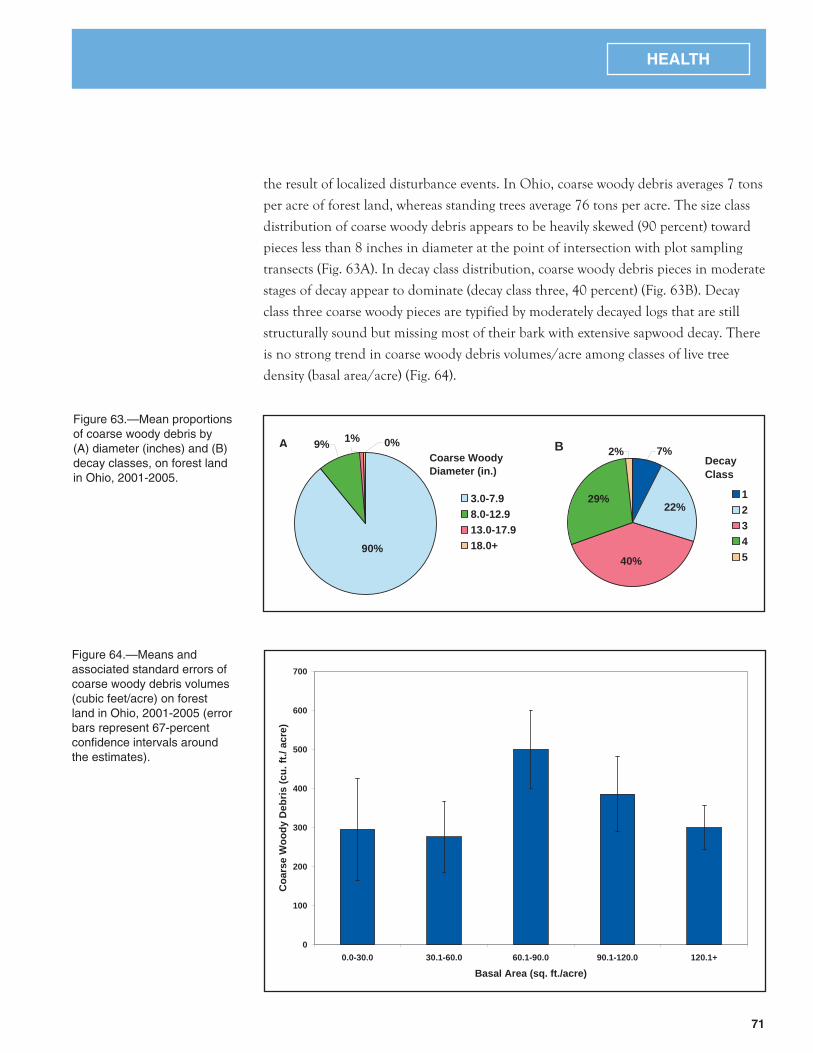
71

HEALTH

Figure 63.—Mean proportions of coarse woody debris by (A) diameter (inches) and (B) decay classes, on forest land in Ohio, 2001-2005.

Figure 64.—Means and associated standard errors of coarse woody debris volumes (cubic feet/acre) on forest land in Ohio, 2001-2005 (error bars represent 67-percent confi dence intervals around the estimates).

the result of localized disturbance events. In Ohio, coarse woody debris averages 7 tons

per acre of forest land, whereas standing trees average 76 tons per acre. The size class

distribution of coarse woody debris appears to be heavily skewed (90 percent) toward

pieces less than 8 inches in diameter at the point of intersection with plot sampling

transects (Fig. 63A). In decay class distribution, coarse woody debris pieces in moderate

stages of decay appear to dominate (decay class three, 40 percent) (Fig. 63B). Decay

class three coarse woody pieces are typified by moderately decayed logs that are still

structurally sound but missing most of their bark with extensive sapwood decay. There

is no strong trend in coarse woody debris volumes/acre among classes of live tree

density (basal area/acre) (Fig. 64).

All live trees =71.0 tons / acsaplings =4.8 /acsalv. Dead= 0.6/ac

1%9%

90%

0%

3.0-7.98.0-12.913.0-17.918.0+

ACoarse WoodyDiameter (in.)

2% 7%

29%22%

40%

12345

BDecayClass

0

100

200

300

400

500

600

700

0.0-30.0 30.1-60.0 60.1-90.0 90.1-120.0 120.1+

Basal Area (sq. ft./acre)

Coa

rse

Woo

dy D

ebris

(cu.

ft./

acre

)

72

HEALTH

The down woody fuel loadings in Ohio’s forests are neither exceedingly high nor

different from those found in neighboring states. Therefore, only in times of extreme

drought would these low amounts of fuels pose a hazard across the State. Of all down

woody components, 1,000+-hr fuels make up the largest amounts. However, coarse

woody debris volumes are still relatively low and were represented by small, moderately

decayed pieces. Overall, because fuel loadings are not exceedingly high across Ohio,

possible fire dangers are outweighed by the benefits of down woody material as wildlife

habitat and carbon sinks.

What this means

Northern hardwoods, snag and large downed woody debris; photo by Steven Katovich, U.S. Forest Service, www.forestryimages.org.

73

HEALTH

Background

What we found

Lichens are composite, symbiotic organisms made up from members of as many as

three kingdoms. The dominant partner is a fungus. Fungi are incapable of producing

their own food, instead providing for themselves as parasites or decomposers.

The lichen fungi (kingdom Fungi) cultivate partners that manufacture food by

photosynthesis. Sometimes the partners are algae (kingdom Protista), other times

cyanobacteria (kingdom Monera), formerly called blue-green algae. Some enterprising

fungi exploit both at once (Brodo et al. 2001).

Lichen community monitoring is included in Forest Health Monitoring to address

issues such as the impact of air pollution on forest resources, or spatial and temporal

trends in biodiversity. This long-term lichen monitoring program in the U.S. dates

back to 1994 and is currently ongoing in 32 states. The objectives of the lichen

indicator are to determine the presence and abundance of lichen species on woody

plants and to collect samples. Lichens occur on many different substrates (e.g., rocks),

but all sampling was restricted to standing trees or branches/twigs that have recently

fallen to the ground. The samples were sent to lichen experts for species identification.

A close relationship exists between lichen communities and air pollution, especially

acidifying or fertilizing nitrogen- and sulfur-based pollutants. A major reason lichens

are so sensitive to air quality is their total reliance on atmospheric sources of nutrition.

In contrast, it is difficult to separate tree-growth responses specific to air pollution

(McCune 2000).

A total of 81 lichen species (gamma diversity) in 29 genera were sampled on the 66

lichen plots (Table 1). The most common lichen genera, Phaeophyscia and Physcia, were

present on 16 and 15 percent of the plots, respectively (Table 2). The genus with the

most species sampled was Cladonia (10 species).

The easiest way to measure species diversity is to count the number of species at a site;

this measure is termed species richness. However, species richness does not provide a

complete picture of diversity in an ecosystem because abundance is excluded. Species

diversity is a concept used to describe the number of different species present in an

area and the distribution of individuals among species. Richness values fell into the

low and medium categories across the State (Table 1). The mean species richness of

the lichen plots was similar across forest-type groups (Table 3). Lichen species richness

was lowest on seedling-sapling plots, which reflect the lag time for lichen recolonization

after harvest or disturbance (Table 4). The spatial distribution of lichen species richness

scores is shown in Figure 65. In general, species richness scores were higher in southern

Ohio. The lichen species richness and diversity scores reported here will serve as

baseline estimates for future monitoring at the State and regional levels.

Lichens

74

HEALTH

Table 1.—Lichen communities summary table for Ohio, 2001-2005

Parameter Ohio, 2001-2005

Number of plots surveyed 66

Number of plots by species richness category0-6 species (low) 177-15 species (medium) 4616-25 species (high) 3

Median species richness score 8.5range of species richness score per plot (low-high) 1-17Average species richness score per plot (alpha diversity) 8.7Standard deviation of species richness score per plot 3.4Species turnover rate (beta diversity)1 9.3Total number of species per area (gamma diversity) 81

1Beta diversity is calculated as gamma diversity divided by alpha diversity

Lichen SpeciesRichness Score

4 - 7

7 - 9

9 - 11

11 - 16

Water

Nonforest

Figure 65.—Estimated lichen species richness, Ohio, 2000-2003.

75

HEALTH

Table 2.—Percentage of specimens and number of

species for lichen genera sampled, Ohio, 2001-2005

Genus All specimens All species

Phaeophyscia 16.0 6Physcia 15.4 5Punctelia 15.0 7Flavoparmelia 9.1 3Myelochroa 8.2 3Parmotrema 7.1 8Parmelia 5.3 3Cladonia 4.7 10Canoparmelia 4.2 3Pyxine 4.1 2Candelaria 3.9 1Heterodermia 1.4 2Parmelinopsis 1.0 2Hypotrachyna 0.9 5Imshaugia 0.5 2Physciella 0.5 1Usnea 0.5 3Cetraria 0.4 1Physconia 0.4 3Flavopunctelia 0.2 2Melanelia 0.2 1Anaptychia 0.1 1Bryoria 0.1 1Leptogium 0.1 1Parmeliopsis 0.1 1Ramalina 0.1 1Rimelia 0.1 1Xanthoria 0.1 1unknown 0.1 1Total 100.0 81

76

HEALTH

Table 4.—Number of FIA Phase 3 plots and richness, diversity, and summation of lichen species by stand-size

categories, with associated sampling errors at the 67-percent confi dence level, Ohio, 2001-2005

Stand size N Species richness SE Diversity SE Summation SE

Seedling/sapling 6 7.7 1.7 1.79 0.37 21.7 5.0Poletimber 25 9.1 0.8 2.04 0.12 24.4 2.4Sawtimber 35 8.5 0.4 2.06 0.05 22.5 1.1All 66 8.7 0.4 2.00 0.06 23.2 1.2

Due to the sensitivity of many lichen species to airborne pollution, it is useful to

look at acid deposition levels. Showman and Long (1992) reported that mean lichen

species richness was significantly lower in areas of high sulfate deposition than in low

deposition areas in north-central Ohio. Sulfate deposition levels have been relatively

high in Ohio and surrounding states in recent years (Fig. 66). A general pattern of

lower lichen species richness scores in high deposition areas and vice versa is evident

(Fig. 67), but many other factors affect the distribution of lichen species including

intrinsic forest characteristics and long-term changes in climate.

What this means

Table 3.—Number of FIA Phase 3 plots and richness, diversity, and summation of lichen species by

forest-type groups, with associated sampling errors at the 67-percent confi dence level, Ohio, 2001-2005

Forest-type group N Species richness SE Diversity SE Summation SE

Maple/beech/birch 12 8.8 0.9 2.06 0.15 23.3 2.8Oak/hickory 50 8.7 0.5 2.03 0.07 23.2 1.4Other 4 8.3 1.8 1.97 0.30 22.0 4.9All 66 8.7 0.4 2.00 0.06 23.2 1.2

77

HEALTH

Figure 67.—Estimated lichen species richness, Northeastern U.S., 2000-2003.

Figure 66—Mean sulfate ion wet deposition, 1994-2002. Data source: National Atmospheric Deposition Program.

8 - 13

13 - 17

17 - 22

22 - 26

26 - 30

Water

Nonforest

Sulfate as SO4-2

(mg/ha)

Low

Medium-low

Medium-high

High

Water

Nonforest

Lichen SpeciesRichness

78

HEALTH

Background Rich soils are the foundation of productive forest land, and they are also one of

the major carbon banks. Soils develop in response to several factors (climate, local

vegetation, topography, parent material, and time), and these factors can be used to

identify soil regions related to particular native forests. Today, the forest soil inventory

illustrates the unique niches that different forests now occupy to maximize their

competitive advantage. By identifying the soil properties associated with various forest

types, the data collected by FIA provide critical baseline information to document

changes in forest health resulting from natural or human influences.

The study of soil carbon is in its infancy. We need more measurements quantifying

the soil carbon pool across different land types, and we need more information on

soil carbon flux over time. Annual inventories of FIA soil plots will provide this

type of information. The results presented here are based upon observations at 84

plots throughout Ohio and 96 plots in the similar forests of Pennsylvania and West

Virginia.

Substantial variability exists within the soil regions of Ohio, Pennsylvania, and West

Virginia as forest trees compete for and create specialized niches. Oak/hickory and

the northern hardwood (maple/beech/birch) stands, for example, accumulated more

forest floor material than elm/ash/red maple stands, but these forests in Ohio tended

to accumulate less forest floor material than forests in the two neighboring states (Fig.

68). As a result, the carbon content of the forest floor in Ohio is less than that of

Pennsylvania in similar forest types (Fig. 69). The differences were less consistent in

the mineral soil carbon stocks (Fig. 70). The oak/hickory forest in Ohio stored less

carbon than similar forests in West Virginia, but the northern hardwood forest was

similar to that in neighboring states. In Ohio, forest floor carbon averages 2 tons per

acre, carbon in the top 20 cm (7.9 inches) of mineral soil averages 22 tons per acre,

and carbon in trees averages 39 tons per acre.

The Soil Quality Index (SQI) is designed to combine the distinct physical and

chemical properties of the soil into a single, integrative assessment (Amacher et

al. 2007). Overall soil quality in Ohio is superior to that observed in Pennsylvania

and West Virginia (Fig. 71). This finding can be broken down into two important

components. The northern hardwood forests of Ohio occurred in landscapes with

greater effective cation exchange capacities (more mineral nutrients) (Fig. 72). Even

more importantly, the calcium:aluminum ratio of mineral soils underlying Ohio’s

forests was generally greater than 0.5; that ratio in Pennsylvania, by contrast, was

largely less than 0.5 (Fig. 73).

What we found

Forest Soils

79

HEALTH

Figure 68.—Mean forest fl oor thickness by forest-type group (error bars represent 67-percent confi dence intervals around estimates).

Figure 69.—Mean forest fl oor carbon by forest-type group (error bars represent 67-percent confi dence intervals around estimates).

0 1 2 3 4 5 6

Elm/ash/cottonwood

Maple / beech / birchgroup

Oak / hickory group

Fore

st-ty

pe G

roup .

Forest Floor Thickness (cm)

OhioPennsylvaniaWest Virginia

0 2 4 6 8 10 12 14

Maple/beech/birch

Oak/hickory

Fore

st-ty

pe G

roup

Forest Floor Carbon (megagrams/hectare)

OhioPennsylvaniaWest Virginia

80

HEALTH

Figure 70.—Mean carbon content of forest soils by forest-type group (error bars represent 67-percent confi dence intervals around estimates).

Figure 71.—Soil Quality Index by forest type (error bars represent 67-percent confi dence intervals around estimates).

0 10 20 30 40 50 60 70 80 90

Maple/beech/birch

Oak/hickoryFo

rest

-type

Gro

up

Mineral Soil Carbon, 0-20 cm (megagrams/hectare)

OhioPennsylvaniaWest Virginia

0 10 20 30 40 50 60 70 80 90 100

Maple/beech/birch

Oak/hickory

Fore

st-ty

pe G

roup

Soil Quality Index, 0-10 cm

OhioPennsylvaniaWest Virginia

81

HEALTH

Figure 72.—Mean effective cation exchange by forest type (error bars represent 67-percent confi dence intervals around estimates).

0 2 4 6 8 10 12 14

Maple/beech/birch

Oak/hickoryFo

rest

-type

gro

up

Effective Cation Exchange Capacity (cmolc/kg)

OhioPennsylvaniaWest Virginia

Figure 73.—Mean ratio of calcium to aluminum by state.

0

10

20

30

40

50

60

70

0 - 0.2 0.2 - 0.5 0.5 - 1.0 1.0 - 1.5 More than 1.5

Ca:Al Molar Ratio, 0-10 cm mineral soil

Rel

ativ

e Fr

eque

ncy

(per

cent

)

OhioPennsylvaniaWest Virginia

82

HEALTH

The forest floor develops from the slow accumulation of organic matter. Carbon is

the primary component of soil organic matter, which has a number of important

functions. These include increasing water holding capacity, retaining some nutrients

by cation exchange (e.g., Ca2+, Mg2+, K+), releasing other nutrients as it decays

(e.g., nitrogen, phosphorus, and sulfur), and capturing potential toxic agents (e.g.,

mercury) (McBride 1994). Carbon is also inventoried to track the sequestration of

certain greenhouse gases. It traps nutrients and improves water holding capacity.

Thicker forest floors contribute toward greater carbon storage. Direct measurements

of carbon and the functions it provides are essential in improving our understanding

of the carbon cycle. Given the similarities between carbon stocks in Ohio’s two major

forest types, there is no incentive to convert forests as a means of increasing carbon

sequestration.

Atmospheric deposition of nitrogen and sulfur alters the soil by leaching essential

minerals from it (Driscoll et al. 2001). Historically, the problem of acid deposition

was particularly severe in the upper Ohio River basin (see National Atmospheric

Deposition Program, http://nadp.sws.uiuc.edu/amaps2/), but while the emissions

that lead to acid deposition have declined, the effects persist (Driscoll et al. 2001).

Effective cation exchange capacity (ECEC) is calculated as the sum of five key mineral

elements: sodium, potassium, calcium, magnesium, and aluminum. High ECEC values

are associated with higher fertility. The molar ratio of Ca to Al is a useful indicator

of stress in forest ecosystems, particularly that caused by acid deposition (Cronan and

Grigal 1995), and low Ca:Al ratios (less than 0.5) indicate an increased likelihood of

negative impacts on tree growth. Additionally, deposition of nitrogen increases litter

decay rates (Kuperman 1999) with the potential to negatively affect the forest through

nitrogen saturation (Aber 1992).

What this means

83

HEALTH

Understory vegetation is an important component of most forested ecosystems. The

total number of species and their relative proportions are the results of past stand

history, including natural disturbances and human influences. By looking at diversity

and abundance of vascular plant species, we may see indications of stresses such as

pollution or forest site degradation. Another indicator of disturbance is an increase

in the number of exotic plants, many of which are early colonizers. FIA assessed

understory vegetation by examining all vascular plants on the forested portion Phase

3 plots during the growing seasons in 2001-2005, about one-sixteenth of the total

forested plots in the State.

On a total of 75 Phase 3 plots in Ohio in this inventory, FIA found 609 different

species and undifferentiated genera of vascular plants. Of this total, 228 were forbs or

herbs, based on their categorization by the PLANTS database of the USDA Natural

Resources Conservation Service (Table 5). Seventy-two were grass or grass-like plants

(graminoids), including grasses, sedges, rushes, arrow-grasses, and quillworts, while 95

Vascular Plants in Ohio’s Forest

Background

What we found

Table 5.—Number of species in Ohio, 2005, by growth habit (per

PLANTS database, USDA Natural Resources Conservation Service)

Growth habitNumber of species or undifferentiated genuses

Forb/herb 228Graminoid 72Shrub 25Shrub, Subshrub, Vine 2Subshrub, Forb/herb 3Subshrub, Shrub 10Subshrub, Shrub, Forb/herb 11Tree 57Tree, Shrub 37Tree, Shrub, Subshrub 1Vine 7Vine, Forb/herb 13Vine, Forb/herb, Subshrub 1Vine, Shrub 2Vine, Subshrub 3Vine, Subshrub, Forb/herb 2Vine, Subshrub, Shrub 2Unclassifi ed 133Total 609

84

HEALTH

were trees. Of the plant species,

380, or 62 percent, were native

to this country while 88, 14

percent, were exotic plants

(Table 6). Poison ivy was the

most common plant species,

found on 71 of the 75 Phase 3

plots in the State (Table 7). The

second most common species

was a non-native invasive,

multiflora rose. Of the top 30 species found on our plots, 12 were tree species.

In 2005, invasive species were prominent in Ohio’s forests. Besides the

abovementioned multiflora rose (Fig. 74), garlic mustard (Fig. 75) and Japanese

honeysuckle (Fig. 76) were also found in a substantial portion of our plots. Despite the

concerns of many that non-native bush honeysuckles were devastating to the region’s

biodiversity (Luken and Goessling 1995, Luken 1988), we found Amur honeysuckle

Table 6.—Number of species in Ohio, 2005, by domestic

or foreign origin (per PLANTS database, USDA Natural

Resources Conservation Service).

Origin Number of species

Cultivated, or not in the U.S. 3Introduced to U.S. 88Native and Introduced to U.S. 7Native to U.S. 380Probably Introduced to U.S. 1Unclassifi ed 130

Figure 74.—Location of multifl ora rose on Phase 3 vegetation plots in Ohio, 2005.

85

HEALTH

Figure 75.—Location of garlic mustard on Phase 3 vegetation plots in Ohio, 2005.

Multifl ora rose; photo by James H. Miller, U.S. Forest Service, www.forestryimages.org

86

HEALTH

on only a portion of our plots (Fig. 77). The apparent effect of these species on tree

regeneration varied. The number of saplings (overstory tree species 1 to 5 inches in

diameter) averaged 517 trees per acre across the 75 Phase 3 plots. Many of the plots

with invasive species present had more saplings per acre than this, but a few invasive

species—European privet, Amur honeysuckle, and Japanese honeysuckle—coincided

with substantially fewer saplings per acre (Table 8).

Table 7.—The top 30 plant species or undifferentiated

genera or categories found in Ohio; the number of plots

where found (in parentheses) and the mean number of

tree saplings per acre on those plots, Ohio, 2005

Species name Tree saplings per acre

Bitternut hickory (43) 479.94Sedge (47) 555.54White avens (48) 535.55American elm (54) 500.41Graminoid (grass or sedge) (52) 566.57Sugar maple (51) 448.17Grape (63) 535.08Northern red oak (46) 515.23Multifl ora rose (69) 528.95Plant (60) 552.33Virginia creeper (69) 495.41Eastern poison ivy (71) 513.24Mayapple (34) 492.59Black cherry (68) 501.61Violet (57) 518.2Black raspberry (50) 569.82Aster (43) 493.25Goldenrod (54) 522.37Red maple (53) 499.94White ash (53) 527.61Sassafras (40) 454.7Flowering dogwood (44) 549.34Christmas fern (43) 489.34Roundleaf greenbrier (35) 479.51Northern spicebush (39) 483.32White snakeroot (34) 493.05American beech (39) 510.76White oak (41) 519.09Hawthorn (34) 579.95Black oak (36) 506.5

Tree of heaven; photo used with permission by Chris Evans, River to River CWMA, www.forestryimages.org

87

HEALTH

Table 8.—The top 18 non-native plant species found in

Ohio, the number of plots where found (in parentheses),

and the mean number of tree saplings per acre on

those plots, Ohio 2005.

Species name Tree saplings per acre

Garlic mustard (21) 600Timothy (12) 962Multifl ora rose (69) 529Creeping jenny (8) 985Common St. Johnswort (7) 677Tree of heaven (7) 325Queen Anne’s lace (15) 663Asian bittersweet (9) 665Sulphur cinquefoil (16) 591Ground ivy (17) 747Japanese honeysuckle (30) 420Russian olive (5) 1,153Amur honeysuckle (9) 498Japanese barberry (13) 604Oxeye daisy (12) 870White clover (8) 738Orchardgrass (8) 888European privet (11) 333

Amur honeysuckle; photo used with permission by Troy Evans, Eastern Kentucky University, www.forestryimages.org

88

HEALTH

Figure 77—Location of Amur honeysuckle on Phase 3 vegetation plots in Ohio, 2005.

Figure 76—Location of Japanese honeysuckle on Phase 3 vegetation plots in Ohio, 2005.

89

HEALTH

What this means Ohio’s forests are the home of hundreds of vascular plant species. The 609 species

found on FIA forested plots represent a diverse and, in some cases, challenging

resource. The challenging segment of Ohio’s plant diversity is that portion made up

of non-native invasive plants (NNIP). Given the history of natural and human-caused

disturbance and forest types, such as oak-hickory, whose shade intolerance results in

understory growing space that is not completely occupied, we expected to find multiple

relationships between NNIP and forest and site characteristics.

In a study of disturbance factors and NNIP presence in the Midwest (Moser et al.

2009), the authors observed that some species, such as multiflora rose and Japanese

honeysuckle, significantly benefited from lower overstory basal areas, but this

relationship did not apply to other species. Another measure of disturbance, distance

to nearest road, appeared to have a significant negative relationship with non-native

bush honeysuckles such as Amur honeysuckle. This observation implied that either the

disturbed growing space near the road or the road as a surrogate for human presence

had a positive influence that diminished with increasing distance from the road.

In evaluating the presence and influence of non-native invasive plants, the challenge

is in separating the human influence from the ecological. One could easily argue that

these results reflect the heavily disturbed nature of Ohio’s second- and third-generation

forests, which either re-established following abandonment of farm land or pasture

or were influenced by heavily disturbed adjacent land. Invasive species are known to

thrive on sites with more available resources (Richardson and Pyšek 2006).

The characteristics of the landscape that influenced invasive species presence may

also have a significant relationship with homestead choice by settlers. Natural and

human-caused disturbances, coupled with anthropogenic establishment of individual

species, have a lingering influence on Ohio’s forest ecosystem long after they occur.

As with most situations where ecological restoration is the goal, elimination of NNIP

on Ohio’s landscape will require both aggressive treatment to halt the spread of the

species and a considerable investment in ecosystem restoration.

90

HEALTH

The health and condition of forests are influenced by various biotic and abiotic

stressors. Abiotic stressors include drought, flooding, cold temperatures or freeze

injury, nutrient deficiencies, soil physical properties affecting soil moisture and

aeration, and toxic pollutants. Biotic stressors include native or introduced damaging

insects, diseases, invasive plant species, and animals.

Drought is an important stress that frequently precedes or contributes to the onset of

major outbreaks of damaging insects. Seasonal or prolonged droughts have long been

a significant stressor in Ohio. Below normal precipitation occurred in Ohio during

1991 and 1994; alternatively, 1996 and the years 2003-2006 were very wet. On poorly

drained soils, too much moisture stresses trees, particularly species not adapted to these

conditions. These extremes in precipitation can be more devastating when followed by

insect outbreaks; they can also produce conditions that facilitate disease outbreaks.

Invasions by exotic diseases and insects are one of the most important threats to the

productivity and stability of forest ecosystems around the world (Liebhold et al. 1995,

Pimentel et al. 2000, Vitousak et al. 1996). Over the last century, Ohio forests have

been affected by well-known exotic and invasive agents such as Dutch elm disease,

chestnut blight, and gypsy moth (Mattson 1997). Invasions by alien species are known

to result in many community-level direct and indirect effects, including changes in

plant species diversity and richness, community structure, vegetation dynamics, and

plant-animal interactions (Mack et al 2000,. Mooney and Cleland 2001, Parker et al.

1999).

Insect and disease pests, both native and exotic, continue to damage and kill trees in

the State’s forests. Looking at changes in standing dead basal area since 1991, we see

that most major species have remained stable or decreased, although white oak and elm

have increased (Fig. 78). The most common types of damage recorded on trees in Ohio

were decay and vines, 52 and 22 percent of trees, respectively. Grapevines damage trees

by breaking tops and limbs and breaking and twisting boles, thereby reducing tree

growth and quality. However, vines also provide food and cover for many species of

wildlife. Across the State tree crowns are generally healthy for most species (Fig. 79);

only white ash, black cherry, and elm species. have more than 5 percent of their basal

area in the ≥20-percent crown dieback categories. Although the amount of standing

dead appears to be decreasing and crowns are generally healthy, some tree species

in Ohio are facing additional risks from newly introduced insects and diseases that

threaten their long-term health and sustainability. The following comments on forest

tree species highlight the major stresses that pose current and potential problems.

Threats to the Health of Important Tree Species in Ohio

91

HEALTH

Figure 79.—Percent of basal area by crown dieback categories (percent) for selected tree species, Ohio, 2005.

Figure 78.—Percent of standing basal area that is dead for selected tree species and percent change, Ohio, 1991 and 2005.

0 5 10 15 20 25

Elm spp.

White oak

White ash

Black cherry

Hickory

American beech

Sugar maple

Yellow-poplar

Red maple

Northern red oak

Dead Basal Area (percent)

1991

2005

-78%

-37%

-48%

-18%

-41%

-58%

+30%

+3%

+81%

+153%

0.0 10.0 20.0 30.0 40.0 50.0 60.0 70.0 80.0 90.0 100.0

Red maple

Sugar maple

Hickory spp.

White ash

Black cherry

White oak

Yellow-poplar

Northern red oak

American beech

Elm spp.

All species

Trees by Dieback Class (percent)0 1-5 6-20 >20

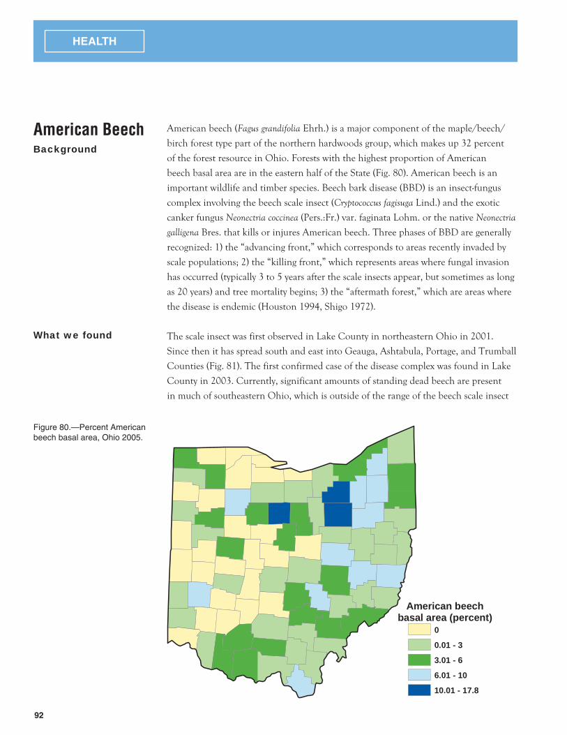
92

HEALTH

American beech (Fagus grandifolia Ehrh.) is a major component of the maple/beech/

birch forest type part of the northern hardwoods group, which makes up 32 percent

of the forest resource in Ohio. Forests with the highest proportion of American

beech basal area are in the eastern half of the State (Fig. 80). American beech is an

important wildlife and timber species. Beech bark disease (BBD) is an insect-fungus

complex involving the beech scale insect (Cryptococcus fagisuga Lind.) and the exotic

canker fungus Neonectria coccinea (Pers.:Fr.) var. faginata Lohm. or the native Neonectria

galligena Bres. that kills or injures American beech. Three phases of BBD are generally

recognized: 1) the “advancing front,” which corresponds to areas recently invaded by

scale populations; 2) the “killing front,” which represents areas where fungal invasion

has occurred (typically 3 to 5 years after the scale insects appear, but sometimes as long

as 20 years) and tree mortality begins; 3) the “aftermath forest,” which are areas where

the disease is endemic (Houston 1994, Shigo 1972).

The scale insect was first observed in Lake County in northeastern Ohio in 2001.

Since then it has spread south and east into Geauga, Ashtabula, Portage, and Trumball

Counties (Fig. 81). The first confirmed case of the disease complex was found in Lake

County in 2003. Currently, significant amounts of standing dead beech are present

in much of southeastern Ohio, which is outside of the range of the beech scale insect

What we found

American BeechBackground

Figure 80.—Percent American beech basal area, Ohio 2005.

American beechbasal area (percent)

0

0.01 - 3

3.01 - 6

6.01 - 10

10.01 - 17.8

93

HEALTH

(Fig. 82). In fact, the amount of

standing dead American beech basal

area has decreased by 2 percent since

the 1991 inventory (Fig. 78). Decay

and vines were noted on 74 and 10

percent of American beech trees,

respectively.

Morin et al. (2007) estimated that

the beech scale is spreading at a

rate of approximately 9.1 miles/

year. The scale insect is expected

to continue spreading into the rest

of Ohio over the next two decades

(Fig. 83). As this spread occurs, it will

be important to continue monitoring for

fungal invasion and subsequent tree mortality. American beech mortality is expected to

increase significantly as the “killing front” of the disease complex advances behind the

“advancing front” of the scale insect.

Figure 81.—Range of the beech scale insect in Ohio, 2006.

Year of BeechScale Invasion

2001

2002

Water

Nonforest

Forest

Beech bark diseaese; photo used with permission Fengyou Jia, Division of Forest Pest Management, DCNR, PA, www.forestryimages.org

What this means

94

HEALTH

Figure 82.—Percent standing dead beech basal area, Ohio 2005.

Figure 83.—Predicted spread of beech scale insect (from Morin et al. 2007).

Dead American beechbasal area (percent)

0

0.01 - 7

7.01 - 15

15.01 - 18

18.01 - 27

95

HEALTH

In Ohio the oak/hickory and oak/pine forest-type groups represent about 56 percent

of forested land area. Forests with the highest proportion of oak (Quercus spp.) basal

area are in the southern and western edges of the

State (Fig. 84). Since 1990, defoliation, primarily

of oaks, by gypsy moth has been a minor pest

problem that may have impacted oak forests by

altering productivity, species composition, and

stand structure in localized areas.

A potential threat to the oak resources in Ohio

is a tree disease called Sudden Oak Death (SOD)

caused by the pathogen Phytophthora ramorum.

Over the past 10 years, large numbers of tanoaks

(Lithocarpus densiflorus), coast live oaks (Quercus agrifolia), and black oaks (Quercus

kelloggii) have been dying in California and Oregon’s coastal counties as a result of

infection. The disease pathogen has also caused leaf blight and shoot dieback on many

other woody and non-woody plant species in these states. P. ramorum has since been

OakBackground

Figure 84.—Percent oak basal area, Ohio 2005.

Oak basalarea (percent)

0 - 5

5.01 - 10

10.01 - 20

20.01 - 35

35.01 - 63

Gypsy moth; photo used with permission by USDA, APHIS PPQ, www.bugwood.org

96

HEALTH

Figure 85.—Numbers of years of gypsy moth defoliation (1990-2002).

inadvertently transported to several eastern states via infected ornamental nursery stock

such as Rhododendron. To date, no nurseries in Ohio have received infected plants, and

forest surveys in nursery perimeters have not detected the pathogen on oaks or any of

the many alternate host species. If the pathogen and disease do arrive, the oak resource

in association with understory hosts such as Rhododendron, Vaccinium, and Kalmia

would be most at risk.

Gypsy moth has defoliated thousands of acres of Ohio’s forests in the past 15 years

(Fig. 85). Mapped estimates of percent standing dead oak basal area are shown in

Figure 86. Decay was the most common form of damage recorded on white, chestnut,

and red oaks (46, 66, and 41 percent, respectively). Vines were most common in red

oak trees (31 percent) but less common in white and chestnut oak (12 and 10 percent,

respectively). Open wounds were recorded on 15 percent of white oak trees. One

possible explanation of this finding is logging damage.

Years of Defoliation1

2

3

Water

Nonforest

Forest

What we found

97

HEALTH

Figure 86.—Percent standing dead oak basal area, Ohio 2005.

What this means Outbreaks of gypsy moth in the 1990s killed trees in localized areas, but this trend was

not picked up with FIA plot data. Although the proportion of white oak basal area

that is dead has increased, this proportion has decreased substantially for northern red

oak (Fig. 78), which may indicate that dead red oak trees have been harvested or fallen

down. Additionally, the crowns of the oak species across the State appear to be healthy

(Fig. 79).

Future defoliation events and the potential arrival of SOD in the eastern United

States are of particular concern to the oak resources in Ohio. Due to the extensive

distribution of overstory hosts of SOD (Fig. 84), this disease could be devastating to

Ohio’s forests. Also of concern is the lack of oak in the smaller diameter classes that

are needed to sustain the oak forest types in the State.

Dead oak basalarea (percent)

0 - 2

2.01 - 7

7.01 - 15

15.01 - 28

28.01 - 52

98

HEALTH

Ash species (Fraxinus spp.) are widely distributed throughout Ohio’s forests but are

rarely a major overstory component (Fig. 87). The elm/ash/maple forest-type group

represents about 7 percent of forested land area in Ohio. Ash is a valuable timber

species, and its seeds are important for many bird species. The two most significant

diseases of ash are ash yellows and ash decline. However, the most significant future

threat to all ash species is the emerald ash borer (EAB) (Agrilus planipennis). EAB is an

exotic insect pest that was first detected in Michigan in 2002 and has since been found

on white and green ash in Indiana, Ohio, and several other places.

Ash yellows and ash decline are likely to be the cause of much of the standing dead ash

in the State (Fig. 88). EAB was first detected in the northwestern corner of Ohio along

the Michigan border. Since it was first discovered in Ohio in 2003, EAB has been

identified in 35 counties (Fig. 89). Presently, the spread of emerald ash borer is being

monitored by the Ohio Department of Agriculture. For the latest quarantine map, go

to the following Web site: http://www.agri.ohio.gov/divs/plant/eab/eabquarantine.

aspx. Decay and vines were noted on 45 and 25 percent of ash trees, respectively.

AshBackground

Figure 87.—Percent ash basal area, Ohio 2005.

Ash basal area(percent)

0 - 4

4.01 - 8

8.01 - 15

15.01 - 22

22.01 - 44

What we found

99

HEALTH

Figure 88.—Percent standing dead ash basal area, Ohio 2005.

Dead ash basalarea (percent)

0 - 1

1.01 - 5

5.01 - 10

10.01 - 20

20.01 - 30

EAB is considered a serious threat because the insect can be inadvertently transported

across state lines in firewood and nursery stock. Counties with EAB have been

quarantined to stop the movement of firewood and ash logs, which are the largest

contributors to the spread of EAB. Emerald ash borer is a lethal pest and will result

in increased ash mortality in both urban and forested landscapes. It will likely cause

significant financial costs to municipalities, property owners, and the forest products

industries in the State. It is hoped that

one or more of the EAB natural enemies

recently found in China will be useful

biocontrol agents. Parasitic wasps that kill

EAB eggs and larvae have been released

at EAB-infested field sites as part of an

ongoing search for tools to manage EAB

populations.

What this means

Emerald ash borer; photo used with permission by David Cappaert, Michigan State University, www.bugwood.org

100

HEALTH

Figure 89.—Known distribution of emerald ash borer.

101

HEALTH

ElmBackground

Figure 90.—Percent elm basal area, Ohio 2005.

Before Dutch elm disease (DED), elms (Ulmus spp.) were a prominent species in Ohio’s

forests, especially in riparian and moist soils, and they were widely planted to provide

a high green canopy over streets in cities and towns. Today, elm species are still widely

distributed throughout Ohio’s forests but are rarely a major overstory component (Fig.

90). The elm/ash/maple forest-type group represents about 7 percent of forested land

area in Ohio. The exotic wilt, Ceratocystis ulmi or Ophiostoma ulmi, commonly known as

Dutch elm disease, was first discovered in North America in Cleveland, Ohio, in 1930.

DED has had a tragic effect on American elms throughout the range of the species.

American elms are now a much less important overstory species than they once were.

DED is likely to be the cause of much of the standing dead elm in Ohio (Fig. 91). Of

the major tree species in the State, elm had the largest amount of basal area in trees

with poor crowns in the latest inventory (Fig. 79). Elm was also the most vine-infested

major species in Ohio (49 percent of trees). Decay was noted on 21 percent of elm

trees.

Elm basal area(percent)

0 - 3

3.01 - 6

6.01 - 9

9.01 - 15

15.01 - 32

What we found

102

HEALTH

What this means

Figure 91.—Percent standing dead elm basal area, Ohio 2005.

Elm is likely to remain a minor overstory component in Ohio’s forests due to the

pervasive effects of DED. The recent increase in elm mortality is likely due to a

new cohort of American elms reaching susceptible age. In Ohio, elms continue to

reproduce and occupy growing space in stands, yet many are killed before they reach

sawtimber size, providing little economic

return. American elm is a prolific seed

producer, and trees as young as 15 years

produce seed (Bey 1990). Because small

elms continue to grow into the resource

base, elm mortality is an ongoing problem.

Elms in natural stands can serve as

reservoirs of elm bark beetles and DED

fungus to infect high value landscape trees

(Haugen 1998). The best management

option for elms may be to eliminate them and manage for alternative species; however,

it may be desirable to retain some elms for biodiversity and aesthetic reasons.

Dead elm basalarea (percent)

0 - 5

5.01 - 15

15.01 - 30

30.01 - 50

50.01 - 89

Dutch elm disease; photo by Joseph O'Brien, U.S. Forest Service, www.bugwood.org

Log pile; photo by Richard Widmann, U.S. Forest Service.Inset: Skidder; photo by Richard Widmann, U.S. Forest Service.

TIMBER PRODUCTS

104

TIMBER PRODUCTS

Background

What we found

FIA, in conjunction with other research units, canvassed primary wood processors

to enumerate the amount of roundwood harvested for products in Ohio, the

types of products produced, and the species used. The harvesting of roundwood

provides income for landowners and the raw material for Ohio’s forest products

industry. Income from the sale of roundwood is often used to subsidize other forest

management activities such as improving access for recreation and enhancing wildlife

habitat, and it helps offset the costs of land ownership. To better manage the State’s

forests, it is important to know the quantity, species, and disposition by product of

wood harvested in Ohio.

A total of 92 million cubic feet of wood was harvested from Ohio’s forests in 2006

and used for products (Fig. 92) (Wiedenbeck 2008). This amount is nearly the same

as the 1989 harvest; however, there was a shift in production from pulpwood to saw

logs. Most wood harvested (66 percent) was used as saw logs and veneer logs in the

production of lumber and veneer. The 60 million cubic feet of saw logs produced

in 2006 (excluding log exports) are equivalent to 411 million board feet, which is

7 percent more than the 382 million board feet produced in 1989. Wood used for

pulpwood and engineered products accounted for 23.5 million cubic feet—26 percent

of the 2006 harvest. This is equivalent to 277,000 cords and is 23 percent less than

the 361,000 cords produced for pulp in 1989. In addition to pulpwood produced

from the harvest of trees for pulp, Ohio typically produces the equivalent of 250,000

cords of sawmill residues that are used as pulp.

Ohio mills import more wood from surrounding

states than is exported. In 2006, 30.0 million

cubic feet of roundwood were received by Ohio

mills from neighboring states, while 12.8 million

cubic feet were shipped to neighboring states.

Most shipments into the State were saw logs and

veneer logs while exports to other states were

predominantly pulpwood.

Nearly all of the saw log harvest is hardwood

species and is predominantly made up of red

oaks, white oaks, yellow-poplar, sugar maple,

black cherry, and red maple: 21, 20, 13, 8, 7, and

6 percent of the total saw log harvest, respectively (Fig. 93). Since 1987, the portion of

the saw log harvest made up of oak species has fallen from 45 to 41 percent while the

portion made up of maples has increased from 8 to 15 percent.

Sawmill; photo by Richard Widmann, U.S. Forest Service

105

TIMBER PRODUCTS

Figure 92.—Roundwood harvest by product, Ohio, 2006.

Figure 93.—Saw log harvest and percentage of total by major species group, Ohio 2006.

56.1

1.3 1.0

30.7

60.3

0.5 1.7

23.5

2.45.2

0

10

20

30

40

50

60

70

Saw logs Veneer logs Misc. products Pulpwood &engineered

products

Exports

Product

Mill

ion

Cub

ic F

eet

1989 2006

0 10 20 30 40 50 60 70 80 90 100

All other species

Beech

Hickory

Ash

Red maples

Black cherry

Sugar maple

Yellow-poplar

White oaks

Red oaks

Million Board Feet

21%

20%

13%

8%

7%

6%

4%

21%

2%

11%

106

TIMBER PRODUCTS

What this means

The number of sawmills processing logs in Ohio declined from 219 mills in 1989 to

197 mills in 2006 (Fig. 94). Most mills that are no longer operating processed less than

a million board feet of log per year although losses occurred across all size classes of

mills. In 2006 more than half the saw logs processed in the State were received at mills

with a capacity of more than 5 million board feet per year, and nearly 30 percent were

received at the eight mills that took in more than 10 million board feet.

Markets for saw logs in Ohio have been strong, as indicated by a stable harvest from

Ohio’s forests since 1989 and log imports into the State continuing to surpassing

exports. However, this may change. In 2005 stumpage prices in Ohio and many other

hardwood producing states fell to 5- year lows (Akers 2006), suggesting changes in the

industrial demand for hardwood saw logs.

The shift in the species composition of the saw log harvest to more maple and less oak

reflects changes in the forest resource. To remain sustainable, the composition of the

harvest will need to continue to shift with changes in the resource.

Having markets for wood is essential to forest management. Despite the loss of some

sawmills and a pulpmill, Ohio’s mills continue to provide landowners a completive

market for their timber. The income landowners receive from selling timber is

an incentive to keep land in forest. It can help pay property taxes and fund forest

management activities such as wildlife habitat improvements and control of invasive

species.

Figure 94.—Number of operating sawmills, 2006 by annual production and percentage of saw logs processed in 2006, Ohio.

98

70

21

83

39

28 29

0

20

40

60

80

100

120

<1 1-4.9 5-9.9=10 Sawmill Size Class (million board feet received)

Number of mills, 2006

Percent of total saw logsprocessed in Ohio, 2006

Sawtimber stand; photo by Richard Widmann, U.S. Forest Service.

Data Sources and Techniques

108

Phase 1

Phase 2

Historically, FIA inventoried each state on a cycle that averaged about 12 years.

However, because of the need for timely and consistent data across large geographical

regions along with national legislative mandates, FIA has changed to an annual

inventory. This system was initiated in Ohio in 2001. Other changes made during the

2001-2006 inventory were the use of new algorithms to assign forest type and stand-

size class to each condition observed on a plot. To make valid comparisons to the

1991 inventory, the 1991 data were used to recalculate previously published estimates

using the new algorithms. In this report, comparisons to the 1991 inventory use these

recalculated estimates.

Phase 1 procedures reduce variance associated with estimates of forest land area. A

statistical estimation technique is used to classify digital satellite imagery and stratify

the land base as forest or nonforest to assign a representative acreage to each sample

plot. Source data are from Landsat Thematic Mapper (30-m resolution) imagery that

ranged from 1999 to 2001. An image filtering technique is used to classify individual

pixels using the 5- by 5-pixel region that surrounds each sample plot. The resulting 26

classes are collapsed for each estimation unit (county or combination of counties with

small areas of forest land). Stratified estimation is applied by assigning each plot to one

of these collapsed strata and by calculating the area of each collapsed stratum in each

estimation unit. Stratified estimation produces more precise estimates than simple

random sampling.

Field measurements are conducted at sample locations situated within individual cells

of a national hexagonal grid laid across Ohio. These sample locations are distributed

about every 3 miles across the landscape. Each Phase 2 sample represents about

6,000 acres depending on the Phase 1 stratification of forest land. The new national

design also incorporates a change to a four-subplot cluster (Fig. 95) (USDA 2002).

At each location, a suite of variables is measured that characterizes the land and trees

associated with the sample. Annually, a set of sample plot locations, referred to as

an “inventory panel,” are measured. Each panel provides an unbiased representation

of conditions across the State. As panels are completed, they can be combined with

existing panels to produce the most precise estimates possible. The Ohio inventory

was initially set up to be on a 7-year (7-panel) cycle. But, after completing 4 panels,

FIA decided to accelerate the inventory to a 5-year cycle. The remaining 3 panels were

completed in the following 2 years. This report is based on the initial measurement

of all panels and plots that make up a complete inventory. Ohio is now on a 5-year

cycle with 20 percent of the plots measured each year. Going forward, new inventory

estimates will be available each year using the most recent complete set of plots.

Forest inventory

109

Phase 3

Figure 95.—FIA Phase 2 and Phase 3 plot design.

More extensive forest health measurements are collected during a 10-week period in

summer on a subset of Phase 2 sample plots. The measurements are grouped into five

general categories of indicators: crown condition, understory vegetation, down woody

material, soil condition, and lichen communities. The intensity of the Phase 3 plots is

one plot per 96,000 acres of land. The relatively small number of Phase 3 samples does

not allow for detailed analyses in some cases. For example, breaking down tree damage

for a particular species by region reduces the number of samples and yields a high

sampling error (SE).

Statistical signifi canceThis report contains a wealth of statistical estimates that are compared over time and

among numerous variables. Changes in estimates are discussed in terms of direction

and magnitude. All mention of “significant” changes are based on comparing

67-percent confidence intervals for the various estimates. If confidence intervals

overlap, there has been no real change in a statistical sense. When confidence intervals

do not overlap, significant change has occurred.

Subplot 1

Subplot 2

Subplot 3Subplot 4

120.0 ft Subplot:24.0 ft radius

Seedling/sapling plot:6.8 ft radius

The 4 subplots are dispersed over an acre

and total 1/6 of an acre in size.

110

The National Woodland Owner survey (www.fia.fs.fed.us/nwos) is conducted annually

by the Forest Service to increase out understanding of private woodland owners—the

critical link between society and forests. Each year, questionnaires are mailed to

individuals and private groups who own the woodlands where FIA has established

inventory plots (Butler et al. 2005). About 6,000 owners are contacted each year.

Results in Ohio are based on 225 responses received during 2002-2006.

The timber products inventory study was a cooperative effort between the Ohio

Department of Natural Resources-Division of Forestry and the Northern Research

Station. The study canvassed all primary wood-using mills within the State using mail

questionnaires designed to determine the size and composition of Ohio’s primary

wood-using industry, its use of roundwood, and its generation and disposition of

wood residues. Division of Forestry personnel contacted nonresponding mills through

additional mailings, telephone calls, and personal contacts. Estimates were made for a

small number of mills that refused all our attempts to obtain their responses. Data on

Ohio’s industrial roundwood receipts have been added to a regional timber removals

database and supplemented with data on out-of-state uses of State roundwood to

provide a complete assessment of Ohio’s timber product output.

National Woodland Owner Survey

Timber Products Inventory

111

Average annual mortality of growing stock: The average

cubic foot volume of sound wood in growing-stock trees

that died in one year.

Average annual net growth of growing stock: The annual

change in cubic foot volume of sound wood in live

sawtimber and poletimber trees, and the total volume of

trees entering these classes through ingrowth, less volume

losses resulting from natural causes.

Average annual removals from growing stock: The

average net growing-stock volume in growing-stock

trees removed annually for roundwood forest products,

in addition to the volume of logging residues and the

volume of other removals due to land use change.

Basal area: Tree area in square feet of the cross section

at breast height of a single tree. When the basal areas

of all trees in a stand are summed, the result is usually

expressed as square feet of basal area per acre.

Bulk density: The mass of soil per unit volume. A

measure of the ratio of pore space to solid materials

in a given soil. Expressed in units of grams per cubic

centimeter of oven dry soil.

Commercial species: Tree species suitable for industrial

wood products.

Compacted live crown ratio: The percent of the total

length of the tree that supports a full, live crown. For

trees that have uneven length crowns, lower branches

should be transferred ocularly to fill holes in the upper

portions of the crown, until a full, even crown is created.

Crown dieback: Recent mortality of branches with fine

twigs, which begins at the terminal portion of a branch

and proceeds toward the trunk. Dieback is considered

only when it occurs in the upper and outer portions of

Glossary

the tree. When whole branches are dead in the upper

crown, without obvious signs of damage such as breaks

or animal injury, the branches are assumed to have died

from the terminal portion of the branch. Dead branches

in the lower portion of the live crown are assumed to

have died from competition and shading. Dead branches

in the lower live crown are not considered part of crown

dieback, unless there is continuous dieback from the

upper and outer crown down to those branches.

Cull tree: Live trees that are unsuitable for the production

of some roundwood products, now or prospectively. Cull

trees can include those with decay (rotten cull) or poor

form, many limbs, or splits (rough cull). Rough cull is

suitable for pulpwood and other fiber products.

Decay class: Qualitative assessment of stage of decay (5

classes) of coarse woody debris based on visual assessments

of color of wood, presence/absence of twigs and branches,

texture of rotten portions, and structural integrity.

Diameter class: A classification of trees based on diameter

outside bark, measured at breast height (d.b.h.) 4.5 feet

(1.37 m) above the ground. Note: Diameter classes are

commonly in 2-inch (5 cm) increments, beginning with

2 inches (5 cm). Each class provides a range of values

with the class name being the approximate mid-point.

For example, the 6-inch class (15-cm class) includes trees

5.0 through 6.9 inches (12.7 through 17.5 cm) d.b.h.,

inclusive.

Down woody material (DWM): DWM, previously named

down woody debris (DWD), is dead material on the

ground in various stages of decay. It includes coarse and

fine wood material. Also measured as part of the DWM

indicator for FIA are the depth of duff layer, litter layer,

and overall fuelbed; fuel loading on the microplot; and

residue piles.

112

Duff: A soil layer dominated by organic material derived

from the decomposition of plant and animal litter and

deposited on either an organic or a mineral surface.

This layer is distinguished from the litter layer in that

the original organic material has undergone sufficient

decomposition that the source of this material (e.g.,

individual plant parts) can no longer be identified.

Effective Cation Exchange Capacity (ECEC): The sum of

cations that a soil can adsorb in its natural pH. Expressed

in units of centimoles of positive charge per kilogram of

soil.

Federal land: An ownership class of public lands owned

by the U.S. Government.

Fiber products: Products derived from wood and bark

residues, such as pulp, composition board products, and

wood chips for export.

Fine woody debris (FWD): Downed, dead branches,

twigs, and small tree or shrub boles <3 inches (7.4 cm) in

diameter not attached to a living or standing dead source.

Forest industry land: An ownership class of private lands

held by a company or individual(s) operating a primary

wood-processing plant.

Forest land: Land at least 10 percent stocked by forest

trees of any size, or land formerly having such tree cover,

and not currently developed for a nonforest use. The

minimum area for classification as forest land is one acre.

Roadside, streamside, and shelterbelt strips of timber

must be at least 120 feet wide to qualify as forest land.

Unimproved roads and trails, streams and other bodies of

water, or natural clearings in forested areas are classified

as forest, if less than 120 feet in width or one acre in

size. Grazed woodlands, reverting fields, and pastures

that are not actively maintained are included if the above

qualifications are satisfied. Forest land includes three

subcategories: timberland, reserved forest land, and other

forest land.

Forest type: A classification of forest land based upon

and named for the tree species that forms the plurality of

live-tree stocking.

Forest-type group: A combination of forest types that

share closely associated species or site requirements.

Major eastern forest-type groups:White-red-jack pine: Forests in which eastern white pine, red pine, or jack pine, singly or in combination, comprise a plurality of the stocking. Common associates include hemlock, aspen, birch, and maple.

Oak-pine: Forests in which hardwoods (usually upland oaks) comprise a plurality of the stocking, but in which pine or eastern redcedar comprises 25-50 percent of the stocking. Common associates include gum, hickory, and yellow-poplar.

Oak-hickory: Forests in which upland oaks or hickory, singly or in combination, comprise a plurality of the stocking except where pines comprise 25-50 percent, in which case the stand is classified as oak-pine. Common associates include yellow-poplar, elm, maple, and black walnut.

Oak-gum-cypress: Bottomland forests in which tupelo, blackgum, sweetgum, oaks, or southern cypress, singly or in combination, comprise a plurality of the stocking except where pines comprise 25-50 percent, in which case the stand is classified as oak-pine. Common associates include cottonwood, willow, ash, elm, hackberry, and maple.

Elm-ash-cottonwood: Forests in which elm, ash, or cottonwood, singly or in combination,

113

comprise a plurality of the stocking. Common associates include willow, sycamore, beech, and maple.

Northern hardwoods (also called maple-beech-birch): Forests in which maple, beech, or yellow birch, singly or in combination, comprise a plurality of the stocking. Common associates include hemlock, elm, basswood, and white pine.

Aspen-birch: Forests in which aspen, balsam poplar, paper birch, or gray birch, singly or in combination, comprise a plurality of the stocking. Common associates include maple and balsam fir.

Growing-stock tree: All live trees 5.0 inches (12.7) cm) in

d.b.h. or larger that meet (now or prospectively) regional

merchantability requirements in terms of saw log length,

grade, and cull deductions. Excludes rough and rotten

cull trees.

Hardwood: Tree species belonging to the botanical

subdivision Angiospermae, class Dicotyledonous, usually

broad-leaved and deciduous.

Industrial wood: All roundwood products, except

firewood.

Land: The area of dry land and land temporarily or partly

covered by water, such as marshes, swamps, and river

flood plains.

Litter: Undecomposed or only partially decomposed

organic material that can be readily identified (e.g., plant

leaves, twigs).

Live cull: A classification that includes live cull trees.

When associated with volume, it is the net volume in live

cull trees that are 5.0 inches in d.b.h. and larger.

Logging residues: The unused portions of trees cut or

destroyed during harvest and left in the woods.

National forest: An ownership class of Federal lands,

designated by Executive order or statute as national

forests or purchase units, and other lands under

the administration of the Forest Service including

experimental areas.

Net volume in cubic feet: The gross volume in cubic

feet less deductions for rot, roughness, and poor form.

Volume is computed for the central stem from a 1-foot

stump to a minimum 4.0-inch top diameter outside bark,

or to the point where the central stem breaks into limbs.

Noncommercial species: Tree species of typically small

size, poor form, or inferior quality, which normally do not

develop into trees suitable for industrial wood products.

Nonforest land: Land that does not support, or has never

supported, forests and lands formerly forested where

use of timber management is precluded by development

for other uses. Includes areas used for crops, improved

pasture, residential areas, city parks, improved roads of

any width and adjoining rights-of-way, powerline clearings

of any width, and noncensus water. If intermingled in

forest areas, unimproved roads and nonforest strips must

be more than 120 feet (36.6 m) wide, and clearings, etc.,

must be more than one acre (0.4 ha) in size to qualify as

nonforest land.

Nonstocked areas: Timberland less than 10 percent

stocked with all live trees.

Other red oaks: A group of species in the genus Quercus

that includes scarlet oak, northern pin oak, southern red

oak, shingle oak, laurel oak, blackjack oak, water oak, pin

oak, willow oak, and black oak.

Ownership: A legal entity having an ownership interest

in land regardless of the number of people involved.

An ownership may be an individual; a combination of

persons; a legal entity such as a corporation, partnership,

114

club, or trust; or a public agency. An ownership has

control of a parcel or group of parcels of land.

Poletimber trees: Live trees at least 5.0 inches in d.b.h.,

but smaller than sawtimber trees.

Primary wood-using mill: A mill that converts

roundwood products into other wood products.

Common examples are sawmills that convert saw logs

into lumber and pulpmills that convert pulpwood into

wood pulp.

Productivity class: A classification of forest land in terms

of potential annual cubic-foot volume growth per acre at

culmination of mean annual increment in fully stocked

natural stands.

Pulpwood: Roundwood, whole-tree chips, or wood

residues used for the production of wood pulp.

Reserved forest land: Land permanently reserved

from wood products utilization through statute or

administrative designation. Examples include national

forest wilderness areas and national parks and

monuments.

Residues: Bark and woody materials that are generated in

primary wood-using mills when roundwood products are

converted to other products. Examples are slabs, edgings,

trimmings, miscuts, sawdust, shavings, veneer cores and

clippings, and pulp screenings. Includes bark residues

and wood residues (both coarse and fine materials) but

excludes logging residues.

Rotten tree: A live tree of commercial species that does

not contain a saw log now or prospectively primarily

because of rot (that is, when rot accounts for more than

50 percent of the total cull volume).

Rough tree: (a) A live tree of commercial species that

does not contain a saw log now or prospectively primarily

because of roughness (that is, when sound cull due to

such factors as poor form, splits, or cracks accounts for

more than 50 percent of the total cull volume) or (b) a

live tree of noncommercial species.

Roundwood products: Logs, bolts, or other round

timber generated from harvesting trees for industrial or

consumer uses. Includes saw logs; veneer and cooperage

logs and bolts; pulpwood; fuelwood; pilings; poles; posts;

hewn ties; mine timbers; and various other round, split,

or hewn products.

Salvable dead tree: A downed or standing dead tree

considered currently or potentially merchantable by

regional standards.

Saplings: Live trees 1.0 to 4.9 inches (2.5 to 12.5 cm) in

diameter (d.b.h/d.r.c.).

Saw log: A log meeting minimum standards of diameter,

length, and defect, including logs at least 8 feet long,

sound and straight, and with a minimum diameter

inside bark of 6 inches for softwoods and 8 inches for

hardwoods, or meeting other combinations of size and

defect specified by regional standards.

Sawtimber tree: A live tree of commercial species

containing at least a 12-foot saw log or two noncontiguous

saw logs 8 feet or longer and meeting regional

specifications for freedom from defect. Softwoods must

be at least 9.0 inches in d.b.h. Hardwoods must be at least

11.0 inches in diameter outside bark (d.o.b.).

Sawtimber volume: Net volume of the saw log portion of

live sawtimber in board feet, International 1/4-inch rule

(unless specified otherwise), from stump to a minimum

7.0-inch top d.o.b. for softwoods and a minimum 9.0-inch

top d.o.b. for hardwoods.

Seedlings: Live trees smaller than 1.0 inch (2.5 cm) in

d.b.h./d.r.c. that are at least 6 inches (15.2 cm) in height

115

for softwoods and 12 inches (30.5 cm) in height for

hardwoods.

Site index: The average total height that dominant and

codominant trees in fully stocked, even-aged stands will

obtain at key ages (usually 25 or 50 years).

Softwood: A coniferous tree, usually evergreen, having

needles or scale-like leaves.

Stand: A group of trees on a minimum of one acre of

forest land that is stocked by forest trees of any size.

Stand-size class: A classification of forest land based

on the size class of all live trees in the area. The classes

include:

Nonstocked: Forest land stocked with less than 10 percent of full stocking with all live trees. Examples are recently cutover areas or recently reverted agricultural fields.

Seedling-sapling: Forest land stocked with at least 10 percent of full stocking with all live trees; half or more of such stocking is in seedlings or saplings or both.

Poletimber: Forest land stocked with at least 10 percent of full stocking with all live trees; half or more of such stocking is in poletimber or sawtimber trees or both, and the stocking of poletimber exceeds that of sawtimber.

Sawtimber: Forest land stocked with at least 10 percent of full stocking with all live trees; half or more of such stocking is in poletimber or sawtimber trees or both, and the stocking of sawtimber is at least equal to that of poletimber.

State land: An ownership class of public lands owned by

states or lands leased by states for more than 50 years.

Stocking: At the tree level, stocking is the density value

assigned to a sampled tree (usually in terms of basal area

per acre), expressed as a percent of the total tree density

required to fully utilize the growth potential of the land.

At the stand level, stocking refers to the sum of the

stocking values of all trees sampled.

Timberland: Forest land that is producing or is capable

of producing crops of industrial wood and not withdrawn

from timber utilization by statute or administrative

regulation. (Note: Areas qualifying as timberland are

capable of producing in excess of 20 cubic feet per acre

per year of industrial wood in natural stands. Currently

inaccessible and inoperable areas are included.)

Timber products output: All timber products cut from

roundwood and byproducts of wood manufacturing

plants. Roundwood products include logs, bolts, or

other round sections cut from growing-stock trees,

cull trees, salvable dead trees, trees on nonforest land,

noncommercial species, sapling-size trees, and limbwood.

Byproducts from primary manufacturing plants include

slabs, edging, trimmings, miscuts, sawdust, shavings,

veneer cores and clippings, and screenings of pulpmills

that are used as pulpwood chips or other products.

Tree size class: A classification of trees based on diameter

at breast height, including sawtimber trees, poletimber

trees, saplings, and seedlings.

Veneer log: A roundwood product from which veneer is

sliced or sawn and that usually meets certain standards of

minimum diameter and length and maximum defect.

116

Aber, J.D. 1992. Nitrogen cycling and nitrogen

saturation in temperate forest ecosystems. Trends in

Ecology and Evolution. 7: 220-223.

Akers, Melody. 2006. Bulletin of hardwood market

statistics: first half 2005. Res. Note NE-386. Newtown

Square, PA: U.S. Department of Agriculture, Forest

Service, Northeastern Research Station. 22 p.

Amacher, M.C.; O’Neil, K.P.; Perry, C.H. 2007. Soil vital

signs: a new Soil Quality Index (SQI) for assessing

forest soil health. Res. Pap. RMRS-RP-65WWW. Fort

Collins, CO: U.S. Department of Agriculture, Forest

Service, Rocky Mountain Research Station. 12 p.

Bey, Calvin F. 1990. Ulmus Americana L., American

Elm. In: Silvics of North America: 2. Hardwoods.

Agric. Hand. 654. Washington, DC: U.S. Department

of Agriculture: 801-807.

Birch, Thomas W. 1996. Private forest-land owners

of the Northern United States, 1994. Resour. Bull.

NE-136. Radnor, PA: U.S. Department of Agriculture,

Forest Service, Northeastern Forest Experiment

Station. 293 p.

Brodo, I.M.; Sharnoff, S.D.; Sharnoff, S. 2001. Lichens

of North America. New Haven, CT: Yale University

Press. 795 p.

Butler, B.J.; Leatherberry, E.C.; Williams, M.S. 2005.

Design, implementation, and analysis methods for

the National Woodland Owner Survey. Gen. Tech.

Rep. NE-336. Newtown Square, PA: U.S. Department

of Agriculture, Forest Service, Northeastern Research

Station. 43 p.

Cronan, C.S.; Grigal, D.F. 1995. Use of calcium/

aluminum ratios as indicators of stress in forest

ecosystems. Journal of Environmental Quality. 24:

209-226.

Dennis, Donald F.; Birch, Thomas W. 1981. Forest

statistics for Ohio-1979. Resour. Bull. NE-68.

Broomall, PA: US. Department of Agriculture, Forest

Service, Northeastern Forest Experiment Station 79. p.

Driscoll, C.T.; Lawrence, G.B.; Bulger, et al. 2001. Acid

rain revisited: advances in scientific understanding

since the passage of the 1970 and 1990 Clean Air Act

Amendments. Hubbard Brook Research Foundation

Science Links Publication, Vol. 1, No. 1. Hanover,

NH: Hubbard Brook Research Foundation. 23 p.

Fralish, James S. 2004. The keystone role of oak and

hickory in the central hardwood forest. In: Spetich,

Martin A., ed. Upland oak ecology symposium: history,

current conditions, and sustainability. Gen. Tech.

Rep. SRS-73. Asheville, NC: U.S. Department of

Agriculture, Forest Service, Southern Research Station:

78-87.

Godman, Richard M. et al. 1990. Acer saccharum

M., Sugar Maple. In: Silvics of North America: 2.

Hardwoods. Agric. Hand. 654. Washington, DC: U.S.

Department of Agriculture: 78-91.

Griffith, Douglas M.; DiGiovanni, Dawn; Witzel,

Teresa; Wharton, Eric H. 1993. Forest statistics

for Ohio, 1991. Resour. Bull. NE 128. Radnor,

PA: US. Department of Agriculture, Forest Service,

Northeastern Forest Experiment Station. 169 p.

Haugen, L. 1998. HOW to identify and manage

Dutch elm disease. NA-PR-07-98. Radnor, PA:

U.S. Department of Agriculture, Forest Service,

Northeastern Area, State and Private Forestry. 26 p.

Literature Cited

117

Houston, D.R. 1994. Major new tree disease epidemics:

beech bark disease. Annual Review of Phytopathology.

32: 75-87.

Hutchison, K.O.; Morgan, J.T. 1956. Ohio’s forests

and wood using industries. Forest Survey Release

19. Columbus, OH: U.S. Department of Agriculture,

Forest Service, Central States Forest Experiment

Station. 40 p.

Kingsley, Neal P.; Mayer, Carl E. 1970. The timber

resources of Ohio. Resour. Bull. NE-19. Upper Darby,

PA: U.S.. Department of Agriculture, Forest Service,

Northeastern Forest Experiment Station. 137 p.

Kuperman, R.G. 1999. Litter decomposition and

nutrient dynamics in oak-hickory forests along a

historic gradient of nitrogen and sulfur deposition.

Soil Biology and Biochemistry. 31: 237-244.

Liebhold, A.M.; Mcdonald, W.M.; Bergdahl, D.; Mastro,

V.C. 1995. Invasion by exotic forest pests: a threat to

forest ecosystems. Forest Science Monograph. 30: 49 p.

Luken, J.O. 1988. Population structure and biomass

allocation of the naturalized shrub Lonicera maackii (Rupr.) Maxim. in forest and open habitats. American

Midland Naturalist. 119(2): 258-267.

Luken J.O.; Goessling, N.1995. Seedling distribution

and potential persistence of the exotic shrub Lonicera maackii in fragmented forests. American Midland

Naturalist. 133(1): 124-130.

Mack, R.N; Simberloff, D.; Lonsdale, W.M.; et al.

2000. Biotic invasions: causes, epidemiology, global

consequences, and control. Ecological Applications.

10: 689-710.

Mattson, W.J. 1997. Exotic insects in North American

forests—ecological systems forever altered. In:

Britton, Kerry O., ed. Proceedings of exotic pests

of eastern forests; 8-10 April 1997; Nashville, TN.

U.S. Department of Agriculture, Forest Service, and

Tennessee Exotic Pest Plant Council, Nashville, TN:

187-193.

McBride, M.B. 1994. Environmental chemistry of soils.

New York: Oxford University Press. 416 p.

McCune, B. 2000. Lichen communities as indicators of

forest health. The Bryologist. 103(2): 353-356.

Mooney, H.A.; Cleland, E.E. 2001. The evolutionary

impact of invasive species. PNAS. 98: 5446-5451.

Morin, Randal S.; Liebhold, A.M.; Tobin, P.C.;

Gottschalk, K.W.; Luzader, E. 2007. Spread of beech

bark disease in the eastern United States and its

relationship to regional forest composition. Canadian

Journal of Forest Research. 37: 726-736.

Moser, W.K.; Hansen M.H.; Nelson, M.D.; Olson C.L.;

McWilliams W.H. 2009. Non-native invasive plant

species in the forests of the Upper Midwest of the

United States. In: Kohli, R.K.; Jose, S.; Batish D.R.;

Singh H.P., eds. Invasive Plants and Forest Ecosystems.

Boca Raton, FL: CRC Press. 29-58.

National Agricultural Statistics Service. on website http://

www.nass.usda.gov/index.asp. (Accessed June 2008).

Nowak, David J.; Walton, Jeffrey T. 2005 Projected

urban growth (2000-2050) and its estimated impact

on the U.S. forest resource. Journal of Forestry. 103

(8): 383-398.

Nowak, David J.; Walton, Jeffrey T.; Dwyer, John

F.; Kaya, Latif G.; Myeong, Soojeong. 2005. The

increasing influence of urban environments on US

forest management. Journal of Forestry. 103(8): 377-

382

118

Parker, I.M.; Simberloff, D.; Lonsdale, W.M.; et al. 1999.

Impact: toward a framework for understanding the

ecological effects of invaders. Biological Invasions. 1:

3-19.

Pimentel, D.; Lach, L.; Zuniga, R.; Morrison, D. 2000.

Environmental and economic costs of nonindigenous

species in the United States. BioScience. 50(1): 53-65.

Richardson, D.M.; Pyšek, P. 2006. Plant invasions:

merging the concepts of species invasiveness

and community invasibility. Progress in Physical

Geography. 30(3): 409-431.

Shigo, A.L. 1972. The beech bark disease today in the

northeastern U.S. Journal of Forestry. 54: 286-289.

Showman, R.E.; Long, R.P. 1992. Lichen studies along a

wet sulfate deposition gradient in Pennsylvania. The

Bryologist. 95(2): 166-170.

U.S. Bureau of Census 2002. http://www.census.gov/

(Accessed June 2008).

U.S. Department of Agriculture, Forest Service. 2002.

Forest inventory and analysis national core field

guide: field data collection procedures for Phase 2

plots, version 3.0. [Online publication]. Washington,

DC: U.S. Department of Agriculture, Forest Service.

http://fia.fs.fed.us/library/field-guides-methods-proc/

(Accessed June 2008).

Vitousek, P.M.; D’Antonio, C.M.; Loope, L.L.;

Westbrooks, R. 1996. Biological invasions as global

environmental change. American Scientist. 84: 468-

478.

Woodall, C.W.; Williams, M.S. 2005. Sampling protocol,

estimation, and analysis procedures for down woody

materials indicator of the FIA program. Gen. Tech.

Rep. NC-256. St. Paul, MN: U.S. Department of

Agriculture, Forest Service, North Central Research

Station. 47 p.

Widmann, R.H.; McWilliams, W.H. 2006. Changes

in the oak resource in the mid-Atlantic states-using

forest inventory and analysis data. In: Proceedings

of the 2006 Society of American Foresters national

convention, our woods: wild and working, 2006. Oct.

25-29, Pittsburgh, PA.

Wiedenbeck, Jan; Sabula, Andy. 2008. Ohio roundwood

utilization by the timber industry in 2006. Resour.

Bull. NRS-32. Newtown Square, PA: U.S. Department

of Agriculture, Forest Service, Northern Research

Station.

119

Oak leaves; photo by Richard Widmann, U.S. Forest Service

About the Authors

RICHARD H. WIDMANN is a Forester with Forest Inventory and Analysis, Northern Research Station, Newtown Square, PA.

DAN BALSER is a Forest Health Specialist with the Ohio Department of Natural Resources—Division of Forestry, Columbus, OH.

CHARLES BARNETT is a Forester with Forest Inventory and Analysis, Northern Research Station, Newtown Square, PA.

BRETT J. BUTLER is a Forester with Forest Inventory and Analysis, Northern Research Station, Amherst, MA.

DOUGLAS M. GRIFFITH is a Forester with Forest Inventory and Analysis, Northern Research Station, Newtown Square, PA.

TONYA W. LISTER is a Research Forester with Forest Inventory and Analysis, Northern Research Station, Newtown Square, PA.

W. KEITH MOSER is a Research Forester with Forest Inventory and Analysis, Northern Research Station, St. Paul, MN.

CHARLES H. PERRY is a Research Soil Scientist with Forest Inventory and Analysis, Northern Research Station, St. Paul, MN.

RACHEL RIEMANN is a Research Forester with Forest Inventory and Analysis, Northern Research Station, Newtown Square, PA.

CHRISTOPHER W. WOODALL is a Research Forester with Forest Inventory and Analysis, Northern Research Station, St. Paul, MN.

The U.S. Department of Agriculture (USDA) prohibits discrimination in all its programs and activities on the basis of race, color, national origin, sex, religion, age, disability, political beliefs, sexual orientation, and marital or family status. (Not all prohibited bases apply to all programs.) Persons with disabilities who require alternative means for communication of program information (Braille, large print, audiotape, etc.) should contact USDA’s TARGET Center at 202-720-2600 (voice and TDD). To fi le a complaint of discrimination, write USDA, Director, Office of Civil Rights, Room 326-W, Whitten Building, 1400 Independence Avenue SW, Washington, DC 20250-9410 or call 202-720-5964 (voice and TDD). USDA is an equal opportunity provider and employer.

Printed on recycled paper

Widmann, Richard H.; Balser, Dan; Barnett, Charles; Butler, Brett J.; Griffith, Douglas M.; Lister, Tonya W.; Moser, W. Keith; Perry, Charles H.; Riemann, Rachel; Woodall, Christopher W. 2009. Ohio forests: 2006. Resour. Bull. NRS-36. Newtown Square, PA: U.S. Department of Agriculture, Forest Service, Northern Research Station. 119 p.

This report summarizes annual forest inventories conducted in Ohio from 2001 to 2006 by the Northern Research Station’s Forest Inventory and Analysis unit. Ohio’s forest land covers 7.9 million acres or 30 percent of the State’s land area, changing little in forest land area since 1991. Of this land, 5.8 million acres (73 percent) are held by family forest owners. The current growing-stock inventory is 12.3 billion cubic feet—2 percent more than in 1991—and averages 1,603 cubic feet per acre. Yellow-poplar continues to lead in volume followed by red and sugar maples. Since 1991, the saw log portion of growing-stock volume has increased by 35 percent to 41 billion board feet. In the latest inventory, net growth exceeded removals for all major species except elm.

KEY WORDS: forest area, forest composition, timber volume, timber growth, timber removals, mortality, forest health, biomass, completed annual inventory