DREXEL UNIVERSITY

CAD EXPERIMENT IV: PHASE SHIFTER Objective: To compare performance of Dispersive and Non-Dispersive Phase Shifters

Olaniyi Q. Jinadu 3/8/2015

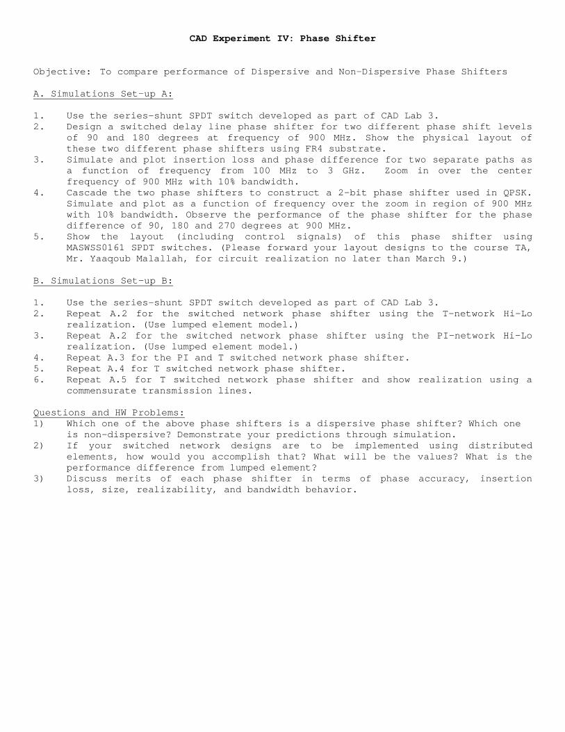
CAD Experiment IV: Phase Shifter Objective: To compare performance of Dispersive and Non-Dispersive Phase Shifters A. Simulations Set-up A: 1. Use the series-shunt SPDT switch developed as part of CAD Lab 3. 2. Design a switched delay line phase shifter for two different phase shift levels

of 90 and 180 degrees at frequency of 900 MHz. Show the physical layout of these two different phase shifters using FR4 substrate.

3. Simulate and plot insertion loss and phase difference for two separate paths as a function of frequency from 100 MHz to 3 GHz. Zoom in over the center frequency of 900 MHz with 10% bandwidth.

4. Cascade the two phase shifters to construct a 2-bit phase shifter used in QPSK. Simulate and plot as a function of frequency over the zoom in region of 900 MHz with 10% bandwidth. Observe the performance of the phase shifter for the phase difference of 90, 180 and 270 degrees at 900 MHz.

5. Show the layout (including control signals) of this phase shifter using MASWSS0161 SPDT switches. (Please forward your layout designs to the course TA, Mr. Yaaqoub Malallah, for circuit realization no later than March 9.)

B. Simulations Set-up B: 1. Use the series-shunt SPDT switch developed as part of CAD Lab 3. 2. Repeat A.2 for the switched network phase shifter using the T-network Hi-Lo

realization. (Use lumped element model.) 3. Repeat A.2 for the switched network phase shifter using the PI-network Hi-Lo

realization. (Use lumped element model.) 4. Repeat A.3 for the PI and T switched network phase shifter. 5. Repeat A.4 for T switched network phase shifter. 6. Repeat A.5 for T switched network phase shifter and show realization using a

commensurate transmission lines. Questions and HW Problems: 1) Which one of the above phase shifters is a dispersive phase shifter? Which one

is non-dispersive? Demonstrate your predictions through simulation. 2) If your switched network designs are to be implemented using distributed

elements, how would you accomplish that? What will be the values? What is the performance difference from lumped element?

3) Discuss merits of each phase shifter in terms of phase accuracy, insertion loss, size, realizability, and bandwidth behavior.

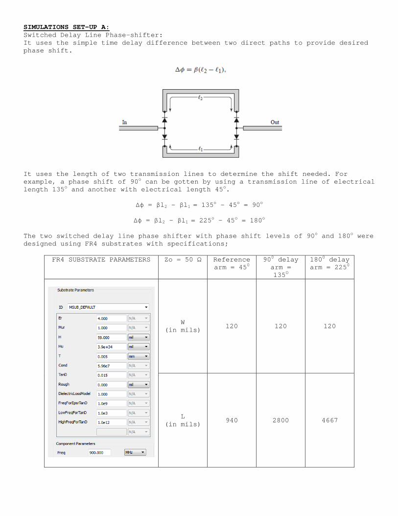
SIMULATIONS SET-UP A: Switched Delay Line Phase-shifter: It uses the simple time delay difference between two direct paths to provide desired phase shift.

It uses the length of two transmission lines to determine the shift needed. For example, a phase shift of 90o can be gotten by using a transmission line of electrical length 135o and another with electrical length 45o.

Δϕ = βl2 – βl1 = 135o – 45o = 90o

Δϕ = βl2 – βl1 = 225o – 45o = 180o

The two switched delay line phase shifter with phase shift levels of 90o and 180o were designed using FR4 substrates with specifications;

FR4 SUBSTRATE PARAMETERS Zo = 50 Ω Reference arm = 450

900 delay arm = 135O

1800 delay arm = 2250

W (in mils) 120 120 120

L (in mils) 940 2800 4667

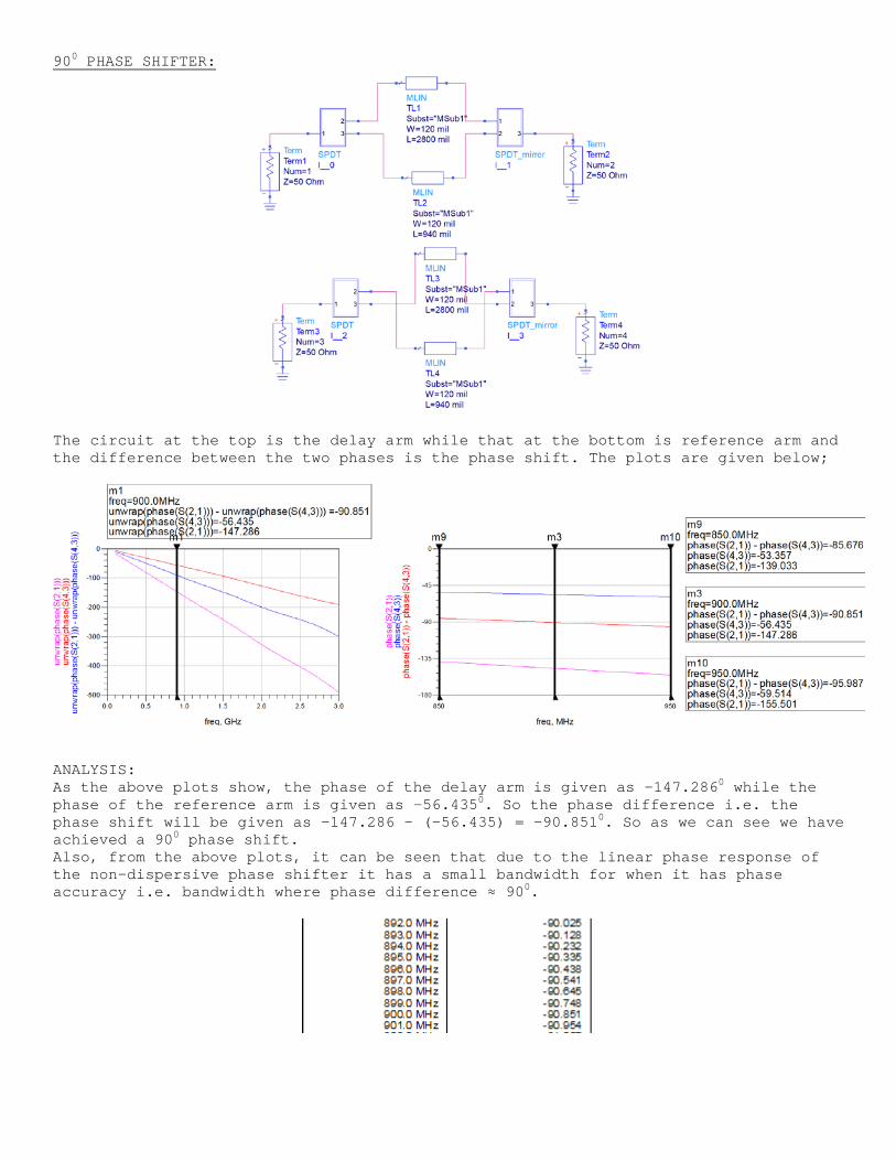
900 PHASE SHIFTER:

The circuit at the top is the delay arm while that at the bottom is reference arm and the difference between the two phases is the phase shift. The plots are given below;

ANALYSIS: As the above plots show, the phase of the delay arm is given as -147.2860 while the phase of the reference arm is given as -56.4350. So the phase difference i.e. the phase shift will be given as -147.286 – (-56.435) = -90.8510. So as we can see we have achieved a 900 phase shift. Also, from the above plots, it can be seen that due to the linear phase response of the non-dispersive phase shifter it has a small bandwidth for when it has phase accuracy i.e. bandwidth where phase difference ≈ 900.

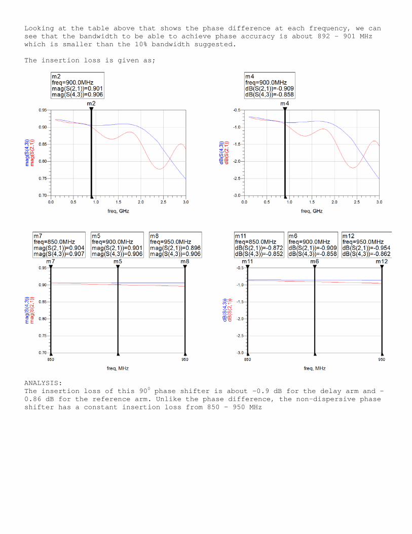
Looking at the table above that shows the phase difference at each frequency, we can see that the bandwidth to be able to achieve phase accuracy is about 892 – 901 MHz which is smaller than the 10% bandwidth suggested. The insertion loss is given as;

ANALYSIS: The insertion loss of this 900 phase shifter is about -0.9 dB for the delay arm and -0.86 dB for the reference arm. Unlike the phase difference, the non-dispersive phase shifter has a constant insertion loss from 850 – 950 MHz

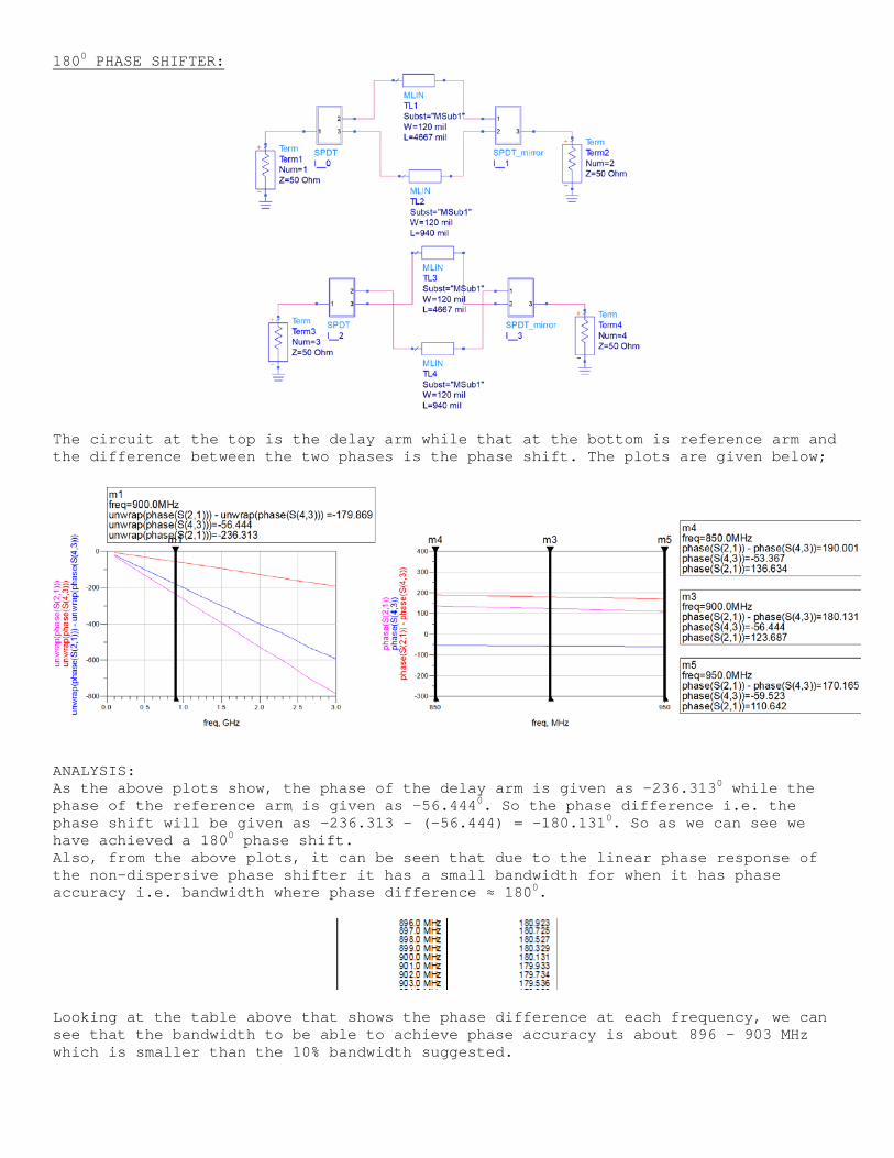
1800 PHASE SHIFTER:

The circuit at the top is the delay arm while that at the bottom is reference arm and the difference between the two phases is the phase shift. The plots are given below;

ANALYSIS: As the above plots show, the phase of the delay arm is given as -236.3130 while the phase of the reference arm is given as -56.4440. So the phase difference i.e. the phase shift will be given as -236.313 – (-56.444) = -180.1310. So as we can see we have achieved a 1800 phase shift. Also, from the above plots, it can be seen that due to the linear phase response of the non-dispersive phase shifter it has a small bandwidth for when it has phase accuracy i.e. bandwidth where phase difference ≈ 1800.

Looking at the table above that shows the phase difference at each frequency, we can see that the bandwidth to be able to achieve phase accuracy is about 896 – 903 MHz which is smaller than the 10% bandwidth suggested.

The insertion loss is given as;

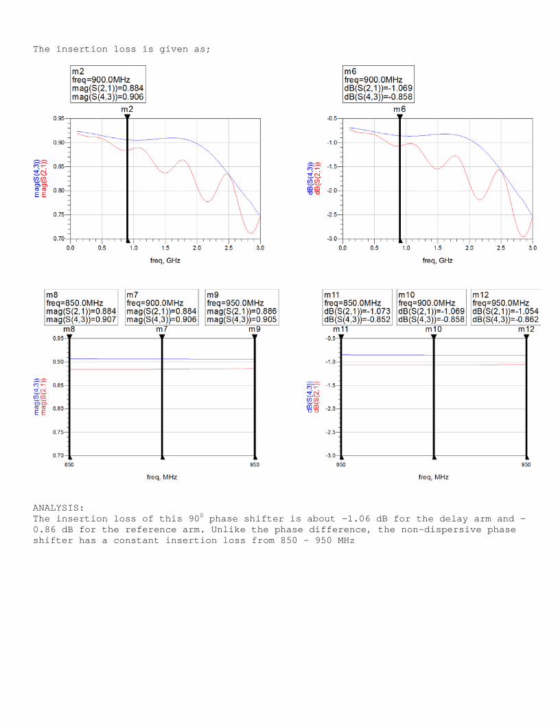
ANALYSIS: The insertion loss of this 900 phase shifter is about -1.06 dB for the delay arm and -0.86 dB for the reference arm. Unlike the phase difference, the non-dispersive phase shifter has a constant insertion loss from 850 – 950 MHz

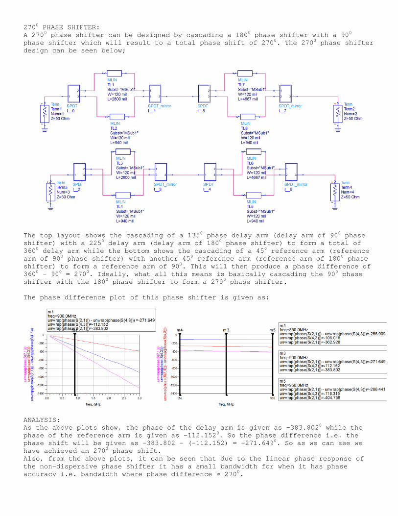
2700 PHASE SHIFTER: A 2700 phase shifter can be designed by cascading a 1800 phase shifter with a 900 phase shifter which will result to a total phase shift of 2700. The 2700 phase shifter design can be seen below;

The top layout shows the cascading of a 1350 phase delay arm (delay arm of 900 phase shifter) with a 2250 delay arm (delay arm of 1800 phase shifter) to form a total of 3600 delay arm while the bottom shows the cascading of a 450 reference arm (reference arm of 900 phase shifter) with another 450 reference arm (reference arm of 1800 phase shifter) to form a reference arm of 900. This will then produce a phase difference of 3600 – 900 = 2700. Ideally, what all this means is basically cascading the 900 phase shifter with the 1800 phase shifter to form a 2700 phase shifter. The phase difference plot of this phase shifter is given as;

ANALYSIS: As the above plots show, the phase of the delay arm is given as -383.8020 while the phase of the reference arm is given as -112.1520. So the phase difference i.e. the phase shift will be given as -383.802 – (-112.152) = -271.6490. So as we can see we have achieved an 2700 phase shift. Also, from the above plots, it can be seen that due to the linear phase response of the non-dispersive phase shifter it has a small bandwidth for when it has phase accuracy i.e. bandwidth where phase difference ≈ 2700.

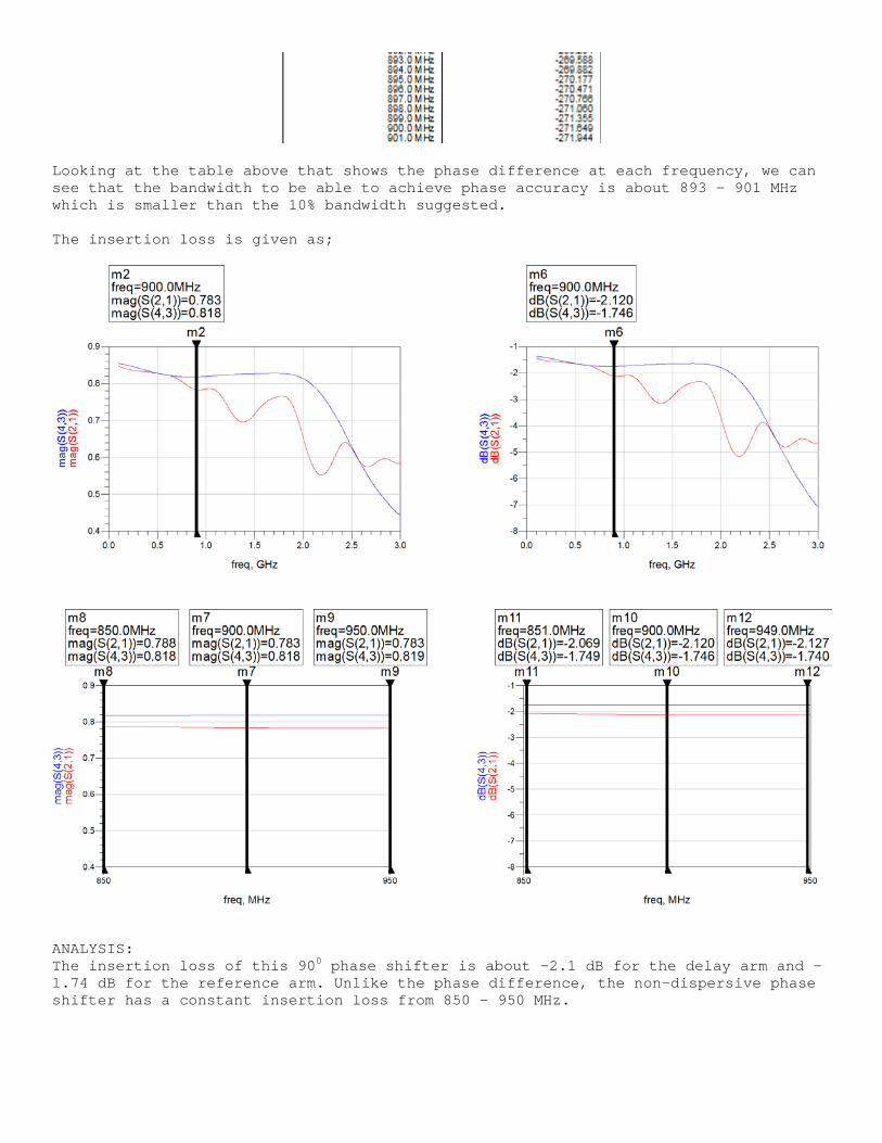
Looking at the table above that shows the phase difference at each frequency, we can see that the bandwidth to be able to achieve phase accuracy is about 893 – 901 MHz which is smaller than the 10% bandwidth suggested. The insertion loss is given as;

ANALYSIS: The insertion loss of this 900 phase shifter is about -2.1 dB for the delay arm and -1.74 dB for the reference arm. Unlike the phase difference, the non-dispersive phase shifter has a constant insertion loss from 850 – 950 MHz.

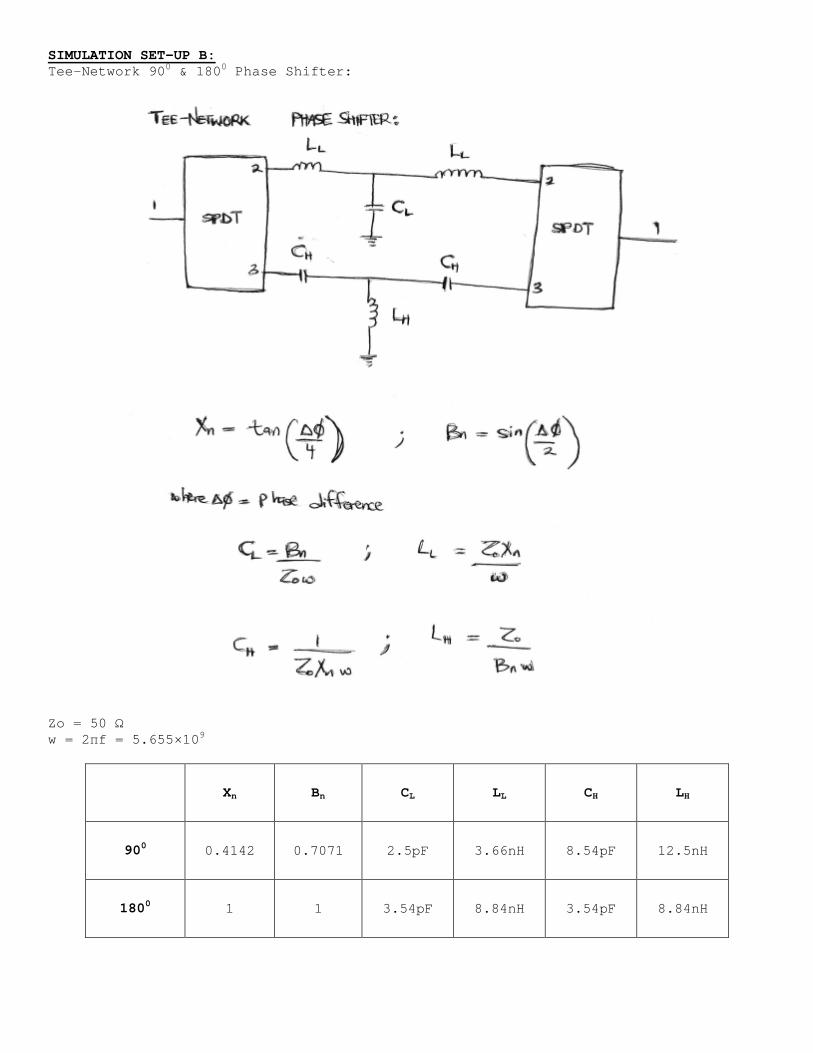
SIMULATION SET-UP B: Tee-Network 900 & 1800 Phase Shifter:

Zo = 50 Ω w = 2πf = 5.655×109

Xn Bn CL LL CH LH

900 0.4142 0.7071 2.5pF 3.66nH 8.54pF 12.5nH

1800 1 1 3.54pF 8.84nH 3.54pF 8.84nH

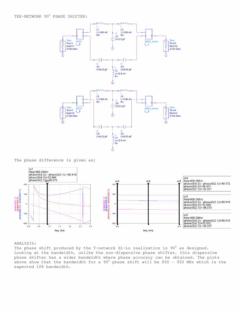
TEE-NETWORK 900 PHASE SHIFTER:

The phase difference is given as;

ANALYSIS: The phase shift produced by the T-network Hi-Lo realization is 900 as designed. Looking at the bandwidth, unlike the non-dispersive phase shifter, this dispersive phase shifter has a wider bandwidth where phase accuracy can be obtained. The plots above show that the bandwidth for a 900 phase shift will be 850 – 950 MHz which is the expected 10% bandwidth.

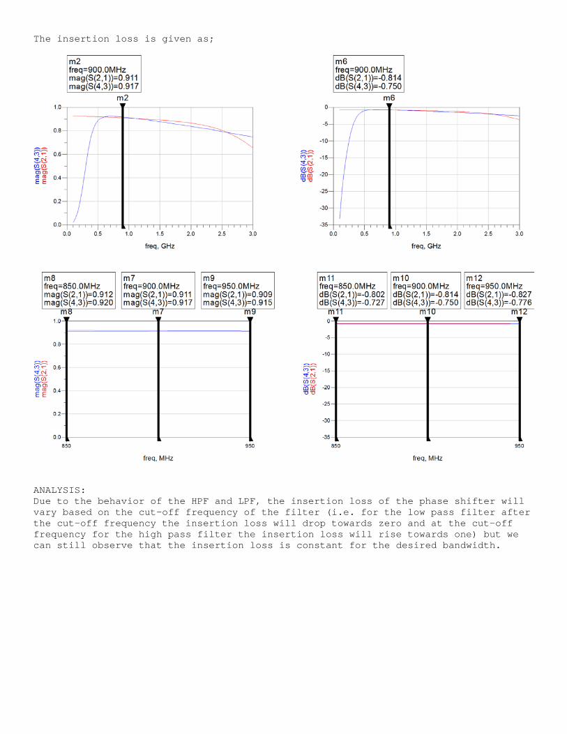
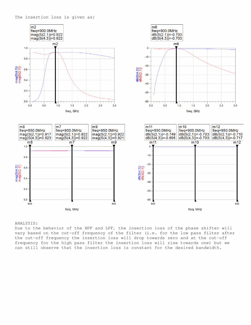
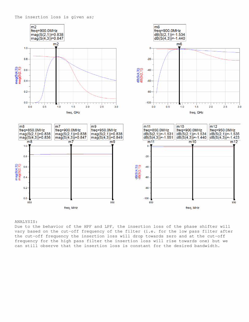
The insertion loss is given as;

ANALYSIS: Due to the behavior of the HPF and LPF, the insertion loss of the phase shifter will vary based on the cut-off frequency of the filter (i.e. for the low pass filter after the cut-off frequency the insertion loss will drop towards zero and at the cut-off frequency for the high pass filter the insertion loss will rise towards one) but we can still observe that the insertion loss is constant for the desired bandwidth.

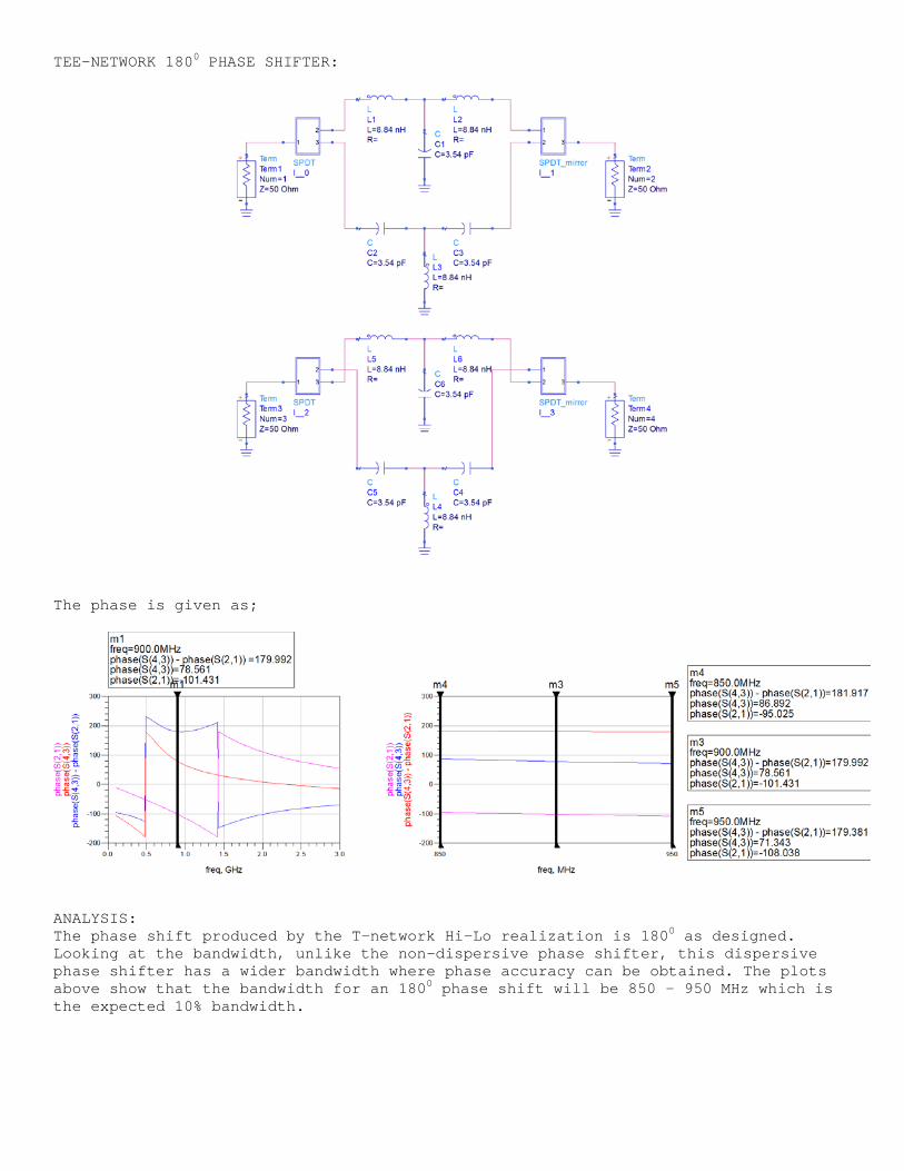
TEE-NETWORK 1800 PHASE SHIFTER:

The phase is given as;

ANALYSIS: The phase shift produced by the T-network Hi-Lo realization is 1800 as designed. Looking at the bandwidth, unlike the non-dispersive phase shifter, this dispersive phase shifter has a wider bandwidth where phase accuracy can be obtained. The plots above show that the bandwidth for an 1800 phase shift will be 850 – 950 MHz which is the expected 10% bandwidth.

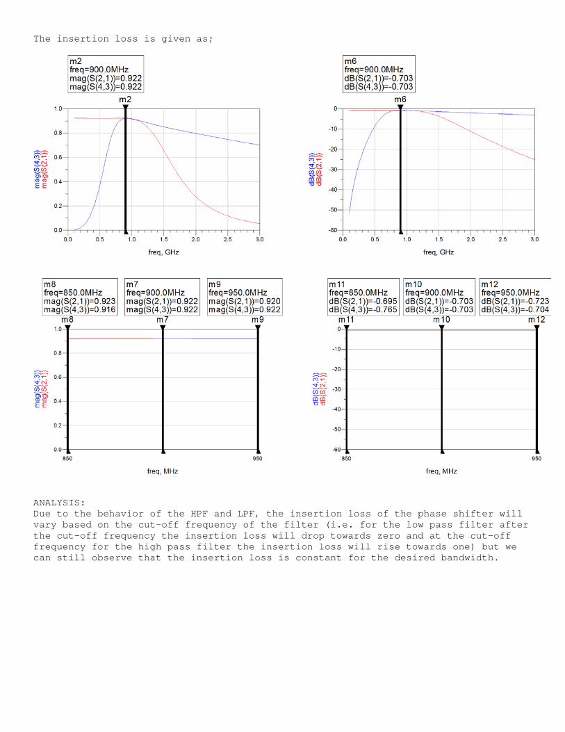
The insertion loss is given as;

ANALYSIS: Due to the behavior of the HPF and LPF, the insertion loss of the phase shifter will vary based on the cut-off frequency of the filter (i.e. for the low pass filter after the cut-off frequency the insertion loss will drop towards zero and at the cut-off frequency for the high pass filter the insertion loss will rise towards one) but we can still observe that the insertion loss is constant for the desired bandwidth.

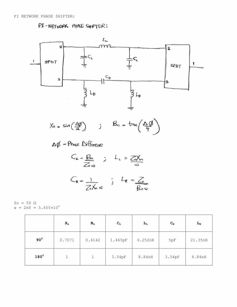
PI NETWORK PHASE SHIFTER:

Zo = 50 Ω w = 2πf = 5.655×109

Xn Bn CL LL CH LH

900 0.7071 0.4142 1.465pF 6.252nH 5pF 21.35nH

1800 1 1 3.54pF 8.84nH 3.54pF 8.84nH

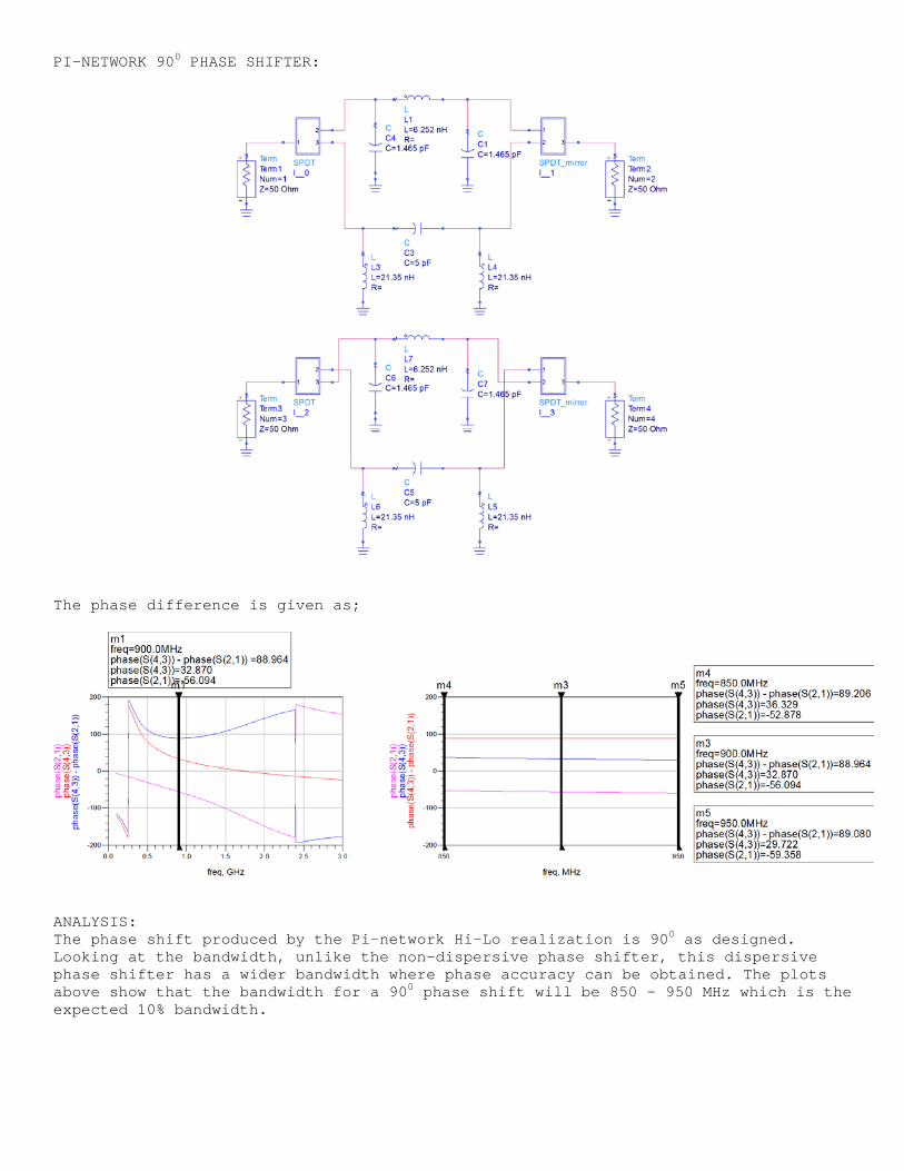
PI-NETWORK 900 PHASE SHIFTER:

The phase difference is given as;

ANALYSIS: The phase shift produced by the Pi-network Hi-Lo realization is 900 as designed. Looking at the bandwidth, unlike the non-dispersive phase shifter, this dispersive phase shifter has a wider bandwidth where phase accuracy can be obtained. The plots above show that the bandwidth for a 900 phase shift will be 850 – 950 MHz which is the expected 10% bandwidth.

The insertion loss is given as;

ANALYSIS: Due to the behavior of the HPF and LPF, the insertion loss of the phase shifter will vary based on the cut-off frequency of the filter (i.e. for the low pass filter after the cut-off frequency the insertion loss will drop towards zero and at the cut-off frequency for the high pass filter the insertion loss will rise towards one) but we can still observe that the insertion loss is constant for the desired bandwidth.

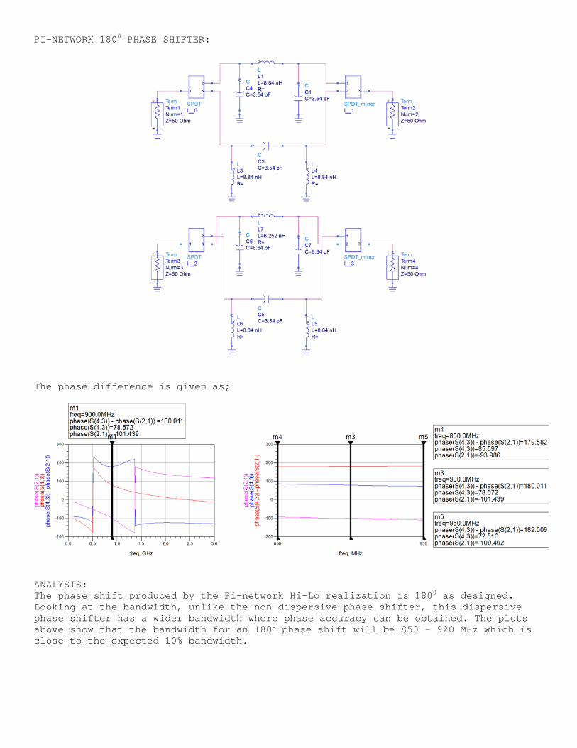
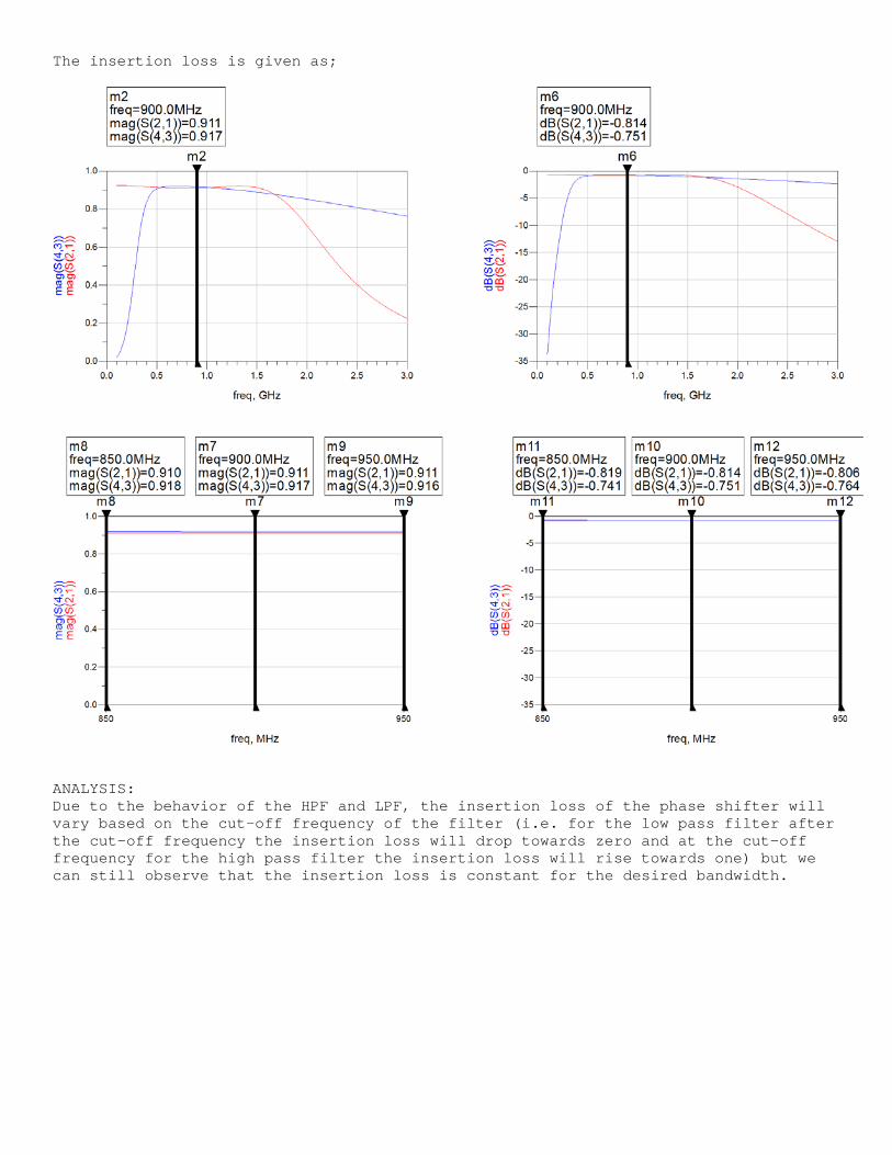
PI-NETWORK 1800 PHASE SHIFTER:

The phase difference is given as;

ANALYSIS: The phase shift produced by the Pi-network Hi-Lo realization is 1800 as designed. Looking at the bandwidth, unlike the non-dispersive phase shifter, this dispersive phase shifter has a wider bandwidth where phase accuracy can be obtained. The plots above show that the bandwidth for an 1800 phase shift will be 850 – 920 MHz which is close to the expected 10% bandwidth.

The insertion loss is given as;

ANALYSIS: Due to the behavior of the HPF and LPF, the insertion loss of the phase shifter will vary based on the cut-off frequency of the filter (i.e. for the low pass filter after the cut-off frequency the insertion loss will drop towards zero and at the cut-off frequency for the high pass filter the insertion loss will rise towards one) but we can still observe that the insertion loss is constant for the desired bandwidth.

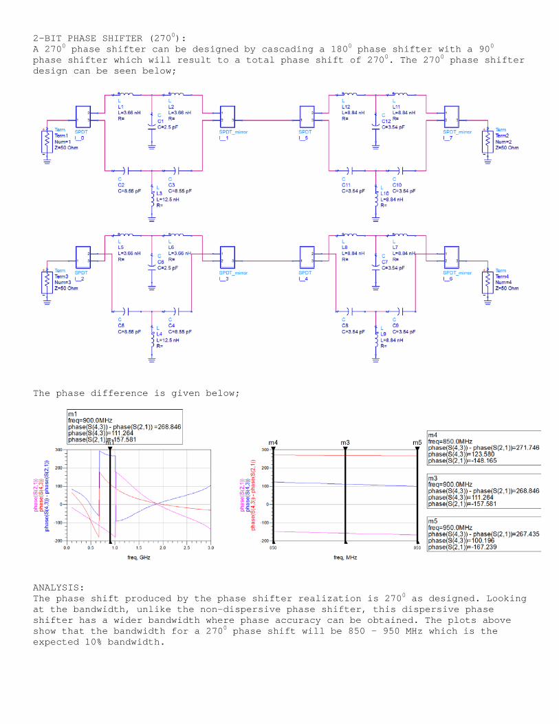
2-BIT PHASE SHIFTER (2700): A 2700 phase shifter can be designed by cascading a 1800 phase shifter with a 900 phase shifter which will result to a total phase shift of 2700. The 2700 phase shifter design can be seen below;

The phase difference is given below;

ANALYSIS: The phase shift produced by the phase shifter realization is 2700 as designed. Looking at the bandwidth, unlike the non-dispersive phase shifter, this dispersive phase shifter has a wider bandwidth where phase accuracy can be obtained. The plots above show that the bandwidth for a 2700 phase shift will be 850 – 950 MHz which is the expected 10% bandwidth.

The insertion loss is given as;

ANALYSIS: Due to the behavior of the HPF and LPF, the insertion loss of the phase shifter will vary based on the cut-off frequency of the filter (i.e. for the low pass filter after the cut-off frequency the insertion loss will drop towards zero and at the cut-off frequency for the high pass filter the insertion loss will rise towards one) but we can still observe that the insertion loss is constant for the desired bandwidth.

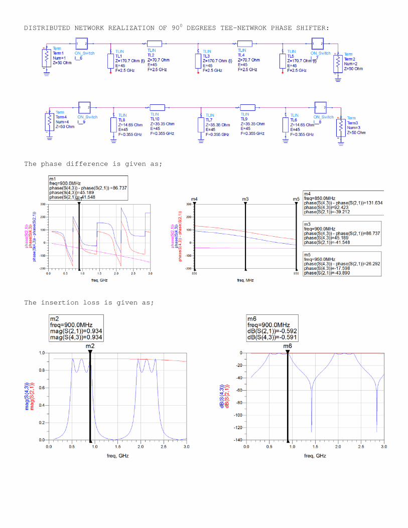
DISTRIBUTED NETWORK REALIZATION OF 900 DEGREES TEE-NETWROK PHASE SHIFTER:

The phase difference is given as;

The insertion loss is given as;

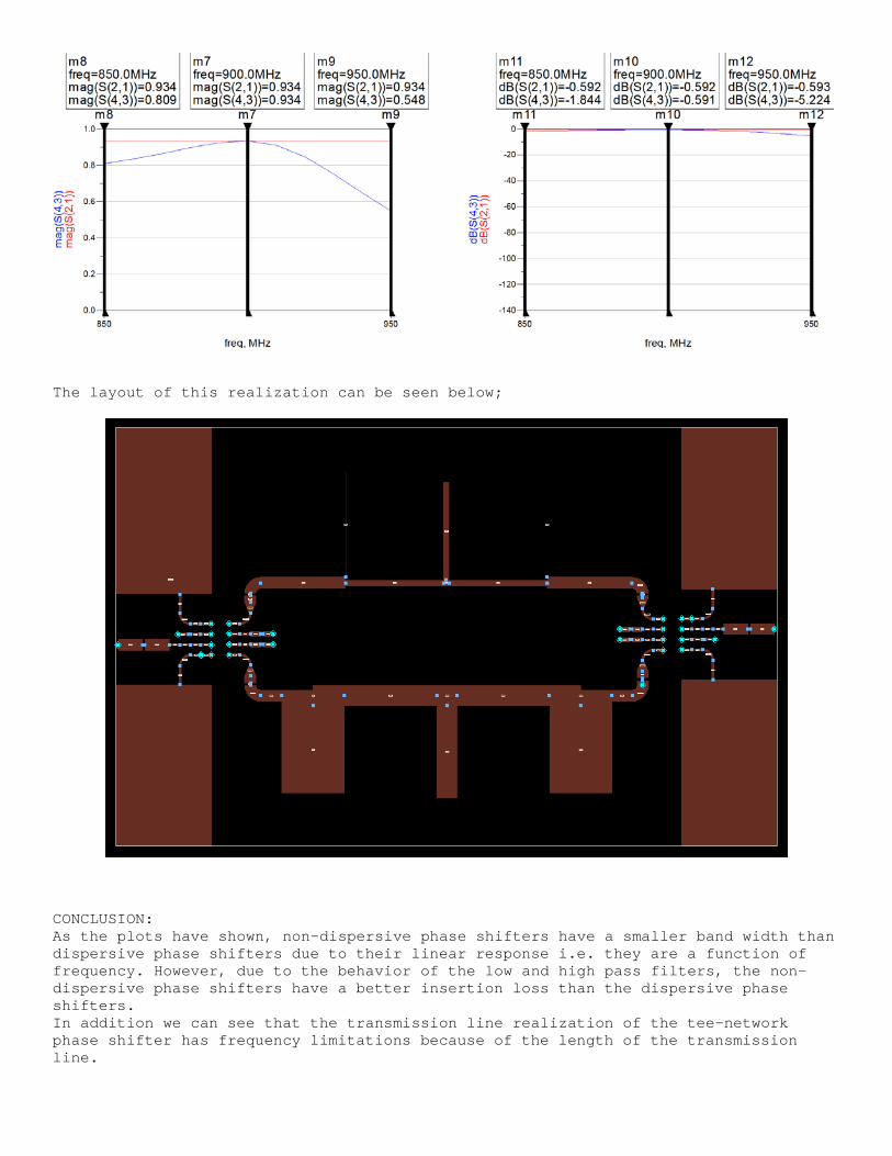
The layout of this realization can be seen below;

CONCLUSION: As the plots have shown, non-dispersive phase shifters have a smaller band width than dispersive phase shifters due to their linear response i.e. they are a function of frequency. However, due to the behavior of the low and high pass filters, the non-dispersive phase shifters have a better insertion loss than the dispersive phase shifters. In addition we can see that the transmission line realization of the tee-network phase shifter has frequency limitations because of the length of the transmission line.

HOMEWORK & QUESTIONS:

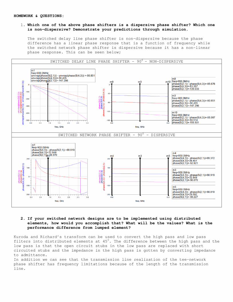
1. Which one of the above phase shifters is a dispersive phase shifter? Which one is non-dispersive? Demonstrate your predictions through simulation.

The switched delay line phase shifter is non-dispersive because the phase difference has a linear phase response that is a function of frequency while the switched network phase shifter is dispersive because it has a non-linear phase response. This can be seen below;

SWITCHED DELAY LINE PHASE SHIFTER - 900 – NON-DISPERSIVE

SWITCHED NETWORK PHASE SHIFTER - 900 - DISPERSIVE

2. If your switched network designs are to be implemented using distributed elements, how would you accomplish that? What will be the values? What is the performance difference from lumped element?

Kuroda and Richard’s transform can be used to convert the high pass and low pass filters into distributed elements at 450. The difference between the high pass and the low pass is that the open circuit stubs in the low pass are replaced with short circuited stubs and the impedance in the high pass is gotten by converting impedance to admittance. In addition we can see that the transmission line realization of the tee-network phase shifter has frequency limitations because of the length of the transmission line.

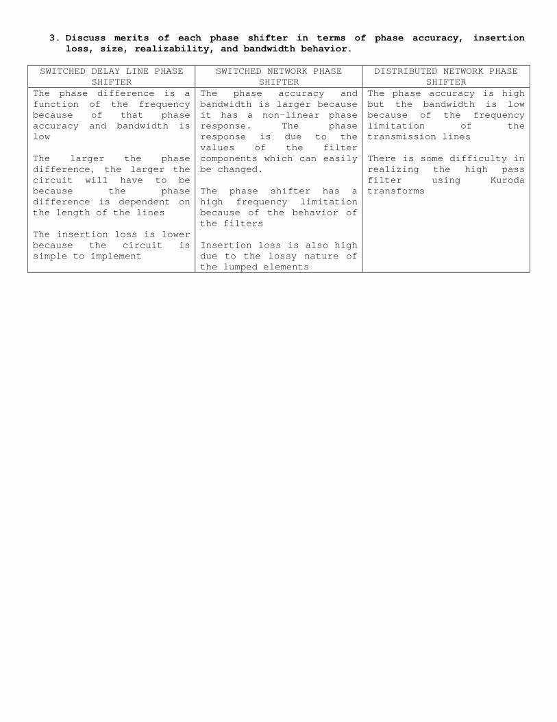
3. Discuss merits of each phase shifter in terms of phase accuracy, insertion loss, size, realizability, and bandwidth behavior.

SWITCHED DELAY LINE PHASE SHIFTER

SWITCHED NETWORK PHASE SHIFTER

DISTRIBUTED NETWORK PHASE SHIFTER

The phase difference is a function of the frequency because of that phase accuracy and bandwidth is low The larger the phase difference, the larger the circuit will have to be because the phase difference is dependent on the length of the lines The insertion loss is lower because the circuit is simple to implement

The phase accuracy and bandwidth is larger because it has a non-linear phase response. The phase response is due to the values of the filter components which can easily be changed. The phase shifter has a high frequency limitation because of the behavior of the filters Insertion loss is also high due to the lossy nature of the lumped elements

The phase accuracy is high but the bandwidth is low because of the frequency limitation of the transmission lines There is some difficulty in realizing the high pass filter using Kuroda transforms