ON A DOMINANCE TEST FOR THE SINGLE MACHINE …archive/pdf/e_mag/Vol.47_02_096.pdf · ON A DOMINANCE TEST FOR THE SINGLE MACHINE SCHEDULING ... Branch-and-bound algorithm is a fundamental

Journal of the Operations ResearchSociety of Japan

2004, Vol. 47, No. 2, 96-111

ON A DOMINANCE TEST FOR THE SINGLE MACHINE SCHEDULING

PROBLEM WITH RELEASE DATES TO MINIMIZE TOTAL FLOW TIME

Shuzo Yanai Tetsuya FujieKobe University of Commerce

(Received August 13, 2003)

Abstract The dominance test is a bounding operation in branch-and-bound algorithms, where each sub-problem is examined whether it can be terminated or not by comparing, implicitly or explicitly, with anothersubproblem. For a single machine scheduling problem with release dates to minimize total flow time, Chu [5]proposed a branch-and-bound algorithm with a dominance test based on already known and new dominanceproperties and reported that the dominance test works successfully to solve problem instances exactly withup to 100 jobs. On the other hand, a naive combination of these dominance properties may delete all ofthe optimal solutions. The purpose of this paper is to point out such a pitfall and then propose a way toavoid it. Furthermore, new dominance properties based on the property developed by Chu [5] are proposed.Computational experiments are performed to see how often the branch-and-bound algorithm with a naivedominance test fails and to show an effectiveness of our branch-and-bound algorithm.

Keywords: Scheduling, dominance test, branch-and-bound algorithm

1. Introduction

Branch-and-bound algorithm is a fundamental exact solution approach to combinatorialoptimization problems including scheduling problems. It is an enumerative algorithm inwhich a given problem is repeatedly decomposed into several subproblems. Each subproblemis tested by computing a lower bound to the optimal solution value of the subproblem (ifthe given problem is a minimization one). If the lower bound is greater than or equal tothe best solution value obtained until the test, which will be called an incumbent value,then the subproblem can be concluded not to provide a better solution and it is terminated.The dominance test is known as another test for subproblems. While the bounding testcompares a lower bound of a subproblem with an incumbent value, the dominance testcompares a subproblem with an another subproblem. More precisely, when we know thatan optimal solution value of a subproblem is not better than that of an another subproblem,the subproblem can be terminated. Besides these tests, several techniques for reducing thesearch space have been proposed. See, e.g., [3] for the techniques developed for schedulingproblems.

In this paper, we consider dominance tests for a single machine scheduling problemwith release dates to minimize total flow time. Dominance properties for this problemwere proposed in [4,5,6] and were used in branch-and-bound algorithms. In particular,Chu [5] combined some already known and new dominance properties and reported thatthe dominance test works successfully to solve problem instances with up to 100 jobs. Thispaper concerns with a combination of dominance properties.

We first point out that, by a naive combination of dominance properties, we may fail toobtain an optimal solution even if each of them alone is correct. Next, we show that slight

96

© 2004 The Operations Research Society of Japan

Dominance Test for Scheduling Problem 97

modification of the dominance properties is enough for branch-and-bound algorithms to workcorrectly. We further propose some new dominance properties. Computational experimentsare performed to see (i) how often the naive dominance test fails, (ii) which combinationof the dominance properties works effectively, and (iii) how large problem instances ourbranch-and-bound algorithm can solve. The remainder of the paper is organized as follows.In Section 2, we describe the scheduling problem and give some notations which are usedthroughout the paper. Dominance properties are discussed in Section 3. Section 4 devotesto our computational experiments. Finally, concluding remarks are described in Section 5.

2. Single Machine Scheduling Problem with Release Dates

2.1. Problem definition

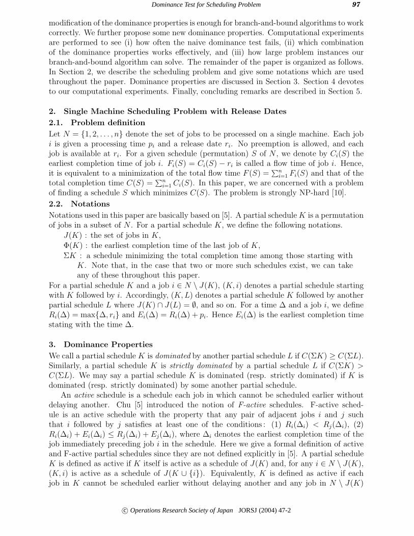
Let N = {1, 2, . . . , n} denote the set of jobs to be processed on a single machine. Each jobi is given a processing time pi and a release date ri. No preemption is allowed, and eachjob is available at ri. For a given schedule (permutation) S of N , we denote by Ci(S) theearliest completion time of job i. Fi(S) = Ci(S) − ri is called a flow time of job i. Hence,it is equivalent to a minimization of the total flow time F (S) =

∑ni=1 Fi(S) and that of the

total completion time C(S) =∑n

i=1 Ci(S). In this paper, we are concerned with a problemof finding a schedule S which minimizes C(S). The problem is strongly NP-hard [10].

2.2. Notations

Notations used in this paper are basically based on [5]. A partial schedule K is a permutationof jobs in a subset of N . For a partial schedule K, we define the following notations.

J(K) : the set of jobs in K,

Φ(K) : the earliest completion time of the last job of K,

ΣK : a schedule minimizing the total completion time among those starting withK. Note that, in the case that two or more such schedules exist, we can takeany of these throughout this paper.

For a partial schedule K and a job i ∈ N \ J(K), (K, i) denotes a partial schedule startingwith K followed by i. Accordingly, (K, L) denotes a partial schedule K followed by anotherpartial schedule L where J(K) ∩ J(L) = ∅, and so on. For a time ∆ and a job i, we defineRi(∆) = max{∆, ri} and Ei(∆) = Ri(∆) + pi. Hence Ei(∆) is the earliest completion timestating with the time ∆.

3. Dominance Properties

We call a partial schedule K is dominated by another partial schedule L if C(ΣK) ≥ C(ΣL).Similarly, a partial schedule K is strictly dominated by a partial schedule L if C(ΣK) >C(ΣL). We may say a partial schedule K is dominated (resp. strictly dominated) if K isdominated (resp. strictly dominated) by some another partial schedule.

An active schedule is a schedule each job in which cannot be scheduled earlier withoutdelaying another. Chu [5] introduced the notion of F-active schedules. F-active sched-ule is an active schedule with the property that any pair of adjacent jobs i and j suchthat i followed by j satisfies at least one of the conditions : (1) Ri(∆i) < Rj(∆i), (2)Ri(∆i) + Ei(∆i) ≤ Rj(∆i) + Ej(∆i), where ∆i denotes the earliest completion time of thejob immediately preceding job i in the schedule. Here we give a formal definition of activeand F-active partial schedules since they are not defined explicitly in [5]. A partial scheduleK is defined as active if K itself is active as a schedule of J(K) and, for any i ∈ N \ J(K),(K, i) is active as a schedule of J(K ∪ {i}). Equivalently, K is defined as active if eachjob in K cannot be scheduled earlier without delaying another and any job in N \ J(K)

c© Operations Research Society of Japan JORSJ (2004) 47-2

98 S. Yanai & T. Fujie

cannot be placed between the jobs in K without delaying them. F-active partial schedulesare defined similarly. It is clear that inactive partial schedules are strictly dominated. Also,partial schedules which are not F-active are strictly dominated (see [5]).

Theorems 3.1-3.5 below are sufficient conditions that the partial schedule (K, i) is dom-inated.

Theorem 3.1 ([4]) Given a partial schedule K and i, j /∈ J(K), i �= j, if Ei(Φ(K)) ≥Ej(Φ(K)) and Ei(Φ(K))−Ej(Φ(K)) ≥ (pi − pj)(|N \ J(K)| − 1), then (K, i) is dominatedby (K, j).

Theorem 3.2 ([4]) Given a partial schedule K and i, j /∈ J(K), i �= j, if Ei(Φ(K)) ≤Ej(Φ(K)) and pi − pj ≤ [Ei(Φ(K)) − Ej(Φ(K))] |N \ J(K)|, then (K, i) is dominated by(K, j).

Theorem 3.3 ([5]) Given a partial schedule K of the form K = (K1, j, K2) and i /∈ J(K),if Ei(Φ(K1)) ≤ Ej(Φ(K1)) and Ei(Φ(K1))−Ej(Φ(K1)) ≤ (pi−pj)|N \J(K)|, then (K, i) =(K1, j, K2, i) is dominated by (K1, i, K2, j).

Theorem 3.4 ([5]) Given a partial schedule K of the form K = (K1, j, K2) and i /∈ J(K),if pi ≥ pj and pi − pj ≥ [Ei(Φ(K1)) − Ej(Φ(K1))] (|J(K2)| + 2), then (K, i) = (K1, j, K2, i)is dominated by (K1, i, K2, j).

Theorem 3.5 ([5]) Given two partial schedules K and K ′, if J(K ′) = J(K), C(K ′) ≤C(K) and |N \ J(K ′)|Rj(Φ(K ′)) + C(K ′) ≤ |N \ J(K)|Rj(Φ(K)) + C(K), where j =arg min{rk : k ∈ N \ J(K ′)} then K is dominated by K ′.

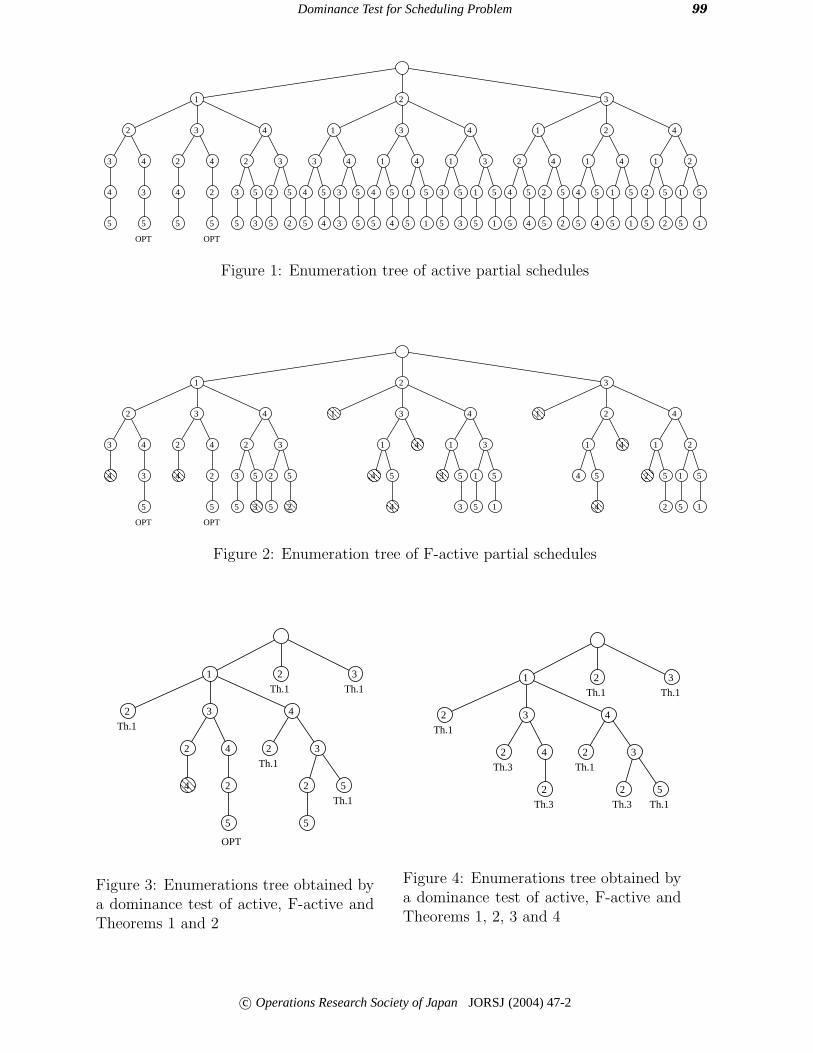
Chu [5] proposed a branch-and-bound algorithm in which the dominance properties ofactive partial schedules, F-active partial schedules and Theorems 3.1-3.5 are used. Each ofthese dominance properties is correct. However, by a naive combination of these properties,we may fail to obtain an optimal solution. For example, consider the problem instance ofn = 5 where ri and pi (i = 1, 2, . . . , 5) are given as follows.

i 1 2 3 4 5ri 0 5 8 12 26pi 9 8 8 1 5

There are two optimal schedules S1 = (1, 2, 4, 3, 5) and S2 = (1, 3, 4, 2, 5) with theminimum total completion time C(S1) = C(S2) = 101. An enumeration tree of activepartial schedules is displayed in Figure 1. In the figure, each node represents a job in aposition which is equal to the depth of the tree, defining the depth of the root node is zero.Hence, each node also represents a partial schedule. All the partial schedules appearing inthe tree are active, and vice versa. OPT denotes that the corresponding schedule is optimal.Figure 2 shows an enumeration tree of F-active partial schedules. Shaded nodes correspondto active but not F-active partial schedules. For instance, a partial schedule (2, 1) is notF-active since (2, 1, 3) is not F-active as a schedule of {1, 2, 3}. In this tree, the two optimalschedules are not deleted (Recall that the active and the F-active partial schedules are strictdominance properties).

Now, let us use Theorems 3.1-3.4 to test whether partial schedules of the form (K, i)are dominated. We suppose the test is performed when (K, i) is generated from K andis proved to be active and F-active. We first apply Theorems 3.1 and 3.2 to the tree inFigure 2. Then we have a tree in Figure 3. For each node dominated by some theorem,the name of the theorem is denoted below the node. We note that the set N \ J(K) isordered to avoid deleting both of the partial schedules (K, i) and (K, j) where (K, i) isdominated by (K, j) and vice versa. In this tree, one of the optimal schedules, S1, is deleted



3

1

1 1

1 1

2 4

2

2

2 1

5 5

5 5

4

4 5

15

5

5 4

2 4

2 5

5 2

4 5

5 4

21

1 3 4

1 3

1 5

5 1

3 5

35

1 4

1 5

5 1

4 5

5 4

3 4

3 5

53

4 5

5 4

2 3 4

2 3

2 5

5 2

3 5

5 3

2 4

2

5

4

5

3 4

3

5

4

5

OPTOPT

Figure 1: Enumeration tree of active partial schedules

3

1

1 1

1

2 4

2

2

2 1

5 5

5

4

4 5

4

21

1 3 4

1 3

1 5

5 1

3 5

3

1 4

4 5

4

2 3 4

2 3

2 5

5 2

3 5

5 3

2 4

2

5

4

3 4

3

5

4

OPTOPT

Figure 2: Enumeration tree of F-active partial schedules

321

2 3 4

2 3

2 5

2 4

2

5

4

Th.1 Th.1

Th.1

Th.1

Th.1

OPT

5

Figure 3: Enumerations tree obtained bya dominance test of active, F-active andTheorems 1 and 2

321

2 3 4

2 3

2 5

2 4

2

Th.1 Th.1

Th.1

Th.1

Th.1Th.3

Th.3

Th.3

Figure 4: Enumerations tree obtained bya dominance test of active, F-active andTheorems 1, 2, 3 and 4



321

2 3 4

2 3

2 5

2 4

2

5

4

Th.1Th.1

Th.1

Th.1

Th.1

OPT

5

Figure 5: Enumeration tree of Figure 3with dominators indicated

321

2 3 4

2 3

2 5

2 4

2

Th.1Th.1

Th.3

Th.1

Th.1

4 3

3 3Th.3

Th.3

Th.3

Figure 6: Enumeration tree of Figure 4with dominators indicated

but the other optimal schedule S2 is not. We then apply Theorems 3.1 and 3.2 followed byTheorems 3.3 and 3.4 to the tree in Figure 2. Then we have a tree in Figure 4 and all of theoptimal schedules are deleted. In this example, even a feasible schedule cannot be obtained.To see why such an incorrect result is produced, one should know dominators by whichpartial schedules are dominated. Figures 5 and 6 displays Figures 3 and 4, respectively,with dominators. In these figures, each broken arrow indicates that the dominance propertyof the theorem shown below the arrow is applied. As Figure 6 shows, (1, 3, 2) and (1, 3, 4, 2)are dominated by (1, 2, 3) and (1, 2, 4, 3), respectively, by Theorem 3.3, both of which aredescendants of the already dominated partial schedule (1, 2). This is the reason why thedominance test fails. Namely, all of the partial schedules which contain optimal schedulesmay be dominated (by Theorem 3.3 or 3.4) by partial schedules whose ancestors are alreadydominated (by Theorem 3.1 or 3.2).

Such an illegal domination might occur since the dominance test of (K, i), which iscompared implicitly with (K, j), can be done without knowing if (K, j) is a descendantof an already dominated partial schedule. Therefore, care has to be taken in using domi-nance properties not only for the problem considered in this paper. For instance, in [8, 9],some conditions that the dominance test has to satisfy are assumed in the study of generalbranch-and-bound algorithms. Of course, the dominance properties considered here doesnot satisfy the conditions. The another way to avoid an illegal domination of (K, i) is toapply the dominance properties with an explicit comparison. This is realized by restrictinga comparison with (K, i) to the one contained in a subproblem pool (a list of unprocessedsubproblems). On the other hand, there is an apparent drawback that scanning subproblemsin the pool is quite time-consuming in general. In this paper, we modify Theorems 3.3–3.5 into Theorems 3.6–3.8 below, where sufficient conditions that a partial schedule (K, i)is strictly dominated are given. Strict dominance properties ensure that partial scheduleswhich contain an optimal solution cannot be deleted by applying them. Hence, by applyingTheorems 3.1 and 3.2 carefully, an optimal solution is always obtained.

Theorem 3.6 (Refinement of Theorem 3.3) Given a partial schedule K of the formK = (K1, j, K2) and i /∈ J(K), if Ei(Φ(K1)) ≤ Ej(Φ(K1)) and Ei(Φ(K1)) − Ej(Φ(K1)) <(pi − pj)|N \ J(K)|, then (K, i) = (K1, j, K2, i) is strictly dominated by (K1, i, K2, j).

Proof : Let Σ(K1, j, K2, i) = (K1, j, K2, i, K3). Then, to prove the theorem, it isenough to show that C(K1, i, K2, j, K3) < C(K1, j, K2, i, K3). For convenience of nota-



tion, let Ck and C ′k denote the completion times of job k in schedules (K1, j, K2, i, K3) and

(K1, i, K2, j, K3), respectively.First suppose pi > pj. Since Ei(Φ(K1)) ≤ Ej(Φ(K1)), we have C ′

k ≤ Ck for k ∈ J(K2).It is clear that ri, rj ≤ Φ(K1, i, K2) ≤ Φ(K1, j, K2). Hence pi > pj implies Φ(K1, i, K2, j) <Φ(K1, j, K2, i) (or, equivalently, C ′

j < Ci). Since then C ′k ≤ Ck for any k ∈ J(K3), we have

C(K1, i, K2, j, K3) < C(K1, j, K2, i, K3).Next suppose pi ≤ pj. Since Ei(Φ(K1)) ≤ Ej(Φ(K1)), we have C ′

k ≤ Ck for k ∈ J(K2),and thus C ′

j − Ci ≤ pj − pi and C ′k − Ck ≤ pj − pi for k ∈ J(K3). Hence, we have

C(K1, i, K2, j, K3) − C(K1, j, K2, i, K3)

= Ei(Φ(K1)) − Ej(Φ(K1)) +∑

k∈J(K2)

(C ′k − Ck) + (C ′

j − Ci) +∑

k∈J(K3)

(C ′k − Ck)

≤ Ei(Φ(K1)) − Ej(Φ(K1)) + (pj − pi) + (pj − pi)|J(K3)|= Ei(Φ(K1)) − Ej(Φ(K1)) − (pi − pj)|N \ J(K)| < 0.

Therefore, (K1, j, K2, i) is strictly dominated by (K1, i, K2, j).

Theorem 3.7 (Refinement of Theorem 3.4) Given a partial schedule K of the formK = (K1, j, K2) and i /∈ J(K), if pi ≥ pj and pi−pj > [Ei(Φ(K1)) − Ej(Φ(K1))] (|J(K2)| + 2),then (K, i) = (K1, j, K2, i) is strictly dominated by (K1, i, K2, j).

Proof : Let Σ(K1, j, K2, i) = (K1, j, K2, i, K3). Then, the proof of Theorem 10 in [5]shows that

C(K1, i, K2, j, K3)−C(K1, j, K2, i, K3) ≤ [Ei(Φ(K1)) − Ej(Φ(K1))] (|J(K2)| + 2)−(pi−pj).

Hence, we have C(K1, i, K2, j, K3) − C(K1, j, K2, i, K3) < 0 and (K1, j, K2, i) is strictlydominated by (K1, i, K2, j).

Theorem 3.8 (Refinement of Theorem 3.5) Given two partial schedules K and K ′, ifJ(K ′) = J(K), C(K ′) ≤ C(K) and |N \J(K ′)|Rj(Φ(K ′))+C(K ′) < |N \J(K)|Rj(Φ(K))+C(K) where j = arg min{rk | k ∈ N \ J(K)}, then K is strictly dominated by K ′.

Proof : If Rj(Φ(K ′)) < Rj(Φ(K)) then it is clear that K is strictly dominated by K ′.Suppose Rj(Φ(K ′)) ≥ Rj(Φ(K)). Let

∑K = (K, L) and C� and C ′

� denote the comple-tion times of job � in (K, L) and (K ′, L), respectively. Then

C(K ′, L) − C(K, L) = C(K ′) − C(K) +∑

�∈N\J(K)

(C ′� − C�)

≤ C(K ′) − C(K) + |N \ J(K)|(Rj(Φ(K ′)) − Rj(Φ(K))) < 0.

Therefore, K is strictly dominated by K ′.

Finally, we propose new dominance properties Theorems 3.9 and 3.10 below, each ofwhich compares two partial schedules (K1, j, K2, i) and (K1, i, K2, j).

Theorem 3.9 Given a partial schedule K of the form K = (K1, j, K2) and i /∈ J(K), ifEi(Φ(K1)) ≤ Ej(Φ(K1)) and Ei(Φ(K1)) − Ej(Φ(K1)) +

∑k∈J(K2)(C

′k − Ck) < (pi − pj)|N \

J(K)|, then (K, i) = (K1, j, K2, i) is strictly dominated by (K1, i, K2, j).

Proof : The proof proceeds in the same way as that of Theorem 3.6.



Theorem 3.10 Given a partial schedule K of the form K = (K1, j, K2) and i /∈ J(K),if Ei(Φ(K1)) ≥ Ej(Φ(K1)) and pj − pi < [Ej(Φ(K1)) − Ei(Φ(K1))](|J(K2)| + 2), then(K, i) = (K1, j, K2, i) is strictly dominated by (K1, i, K2, j).

Proof : Let Σ(K1, j, K2, i) = (K1, j, K2, i, K3) and Ck and C ′k denote the completion

times of job k in schedules (K1, j, K2, i, K3) and (K1, i, K2, j, K3), respectively. By definition,C ′

i = Ei(Φ(K1)) and Cj = Ej(Φ(K1)), and thus C ′i ≥ Cj by the condition. Then we can

show that C ′j − Ci ≤ (C ′

i + pj) − (Cj + pi) holds. Hence it follows that

C ′j − Ci ≤ (pj − pi) + (C ′

i − Cj)

< (pj − pi) + (C ′i − Cj)(|J(K2)| + 2)

< 0,

and thus C ′k ≤ Ck for k ∈ J(K3). Therefore

C(K1, i, K2, j, K3) − C(K1, j, K2, i, K3)

= (C ′i − Cj) +

∑

k∈J(K2)

(C ′k − Ck) + (C ′

j − Ci) +∑

k∈J(K3)

(C ′k − Ck)

≤ (|J(K2)| + 1)(C ′i − Cj) + ((C ′

i + pj) − (Cj + pi))

= (|J(K2)| + 2)(C ′i − Cj) + (pj − pi) < 0,

and (K1, j, K2, i) is strictly dominated by (K1, i, K2, j).

We note that, in Theorems 3.9 and 3.10, (K1, j, K2, i) is dominated by (K1, i, K2, j) if‘<’ is replaced by ‘≤’.

4. Computational Experiments

In this section, we report our computational experiments of the dominance properties dis-cussed in the previous section. In Section 4.1, we describe a branch-and-bound algorithmdeveloped for our experiments. Computational results are reported in Section 4.2, whereit is shown how often Theorems 3 and 4 lead to delete optimal solutions and that whichcombination of the dominance properties is effective in our implementation.

4.1. Branch-and-bound algorithm

A branch-and-bound algorithm used in this section is based on the algorithm, named BB C,developed by Chu [5]. In BB C, a lower bound is an optimal solution value of a relaxationproblem which is obtained by allowing preemption. The relaxation problem is solved by theSRPT (Smallest Remaining Processing Time) rule [2]. In this rule, at any time, a job isselected among those available with the smallest remaining processing time. In [1], Ahmadiand Bagchi compared six lower bounds in the literature and proved that the lower boundbased on the SRPT rule is the dominant both in quality and in time complexity. Heuristicalgorithms used in BB C are those named PRTF and APRTF. In PRTF jobs are orderedaccording to a function PRTF(i, ∆) = Ri(∆) + Ei(∆), while APRTF orders jobs accordingto functions PRTF(i, ∆) and Ri(∆). For a detailed description of these algorithms, see [5].Now, we are ready to state the branch-and-bound algorithm. In the following, L is thesubproblem pool.



Branch-and-Bound Algorithm

Step 0. Let S∗ be a schedule obtained by APRTF and PRTF. Let L := {∅}.Step 1. If L = ∅ then output S∗ and stop. Otherwise, select K ∈ L in a depth-first fashion

and delete it from L.Step 2. If |J(K)| < n − 1 then let A := N \ J(K) and go to Step 3. Otherwise (i.e.,|J(K)| = n − 1), we have a unique schedule (K, i). If C((K, i)) < C(S∗) then letS∗ := (K, i) and update L (that is, delete subproblems, whose lower bound is greaterthan or equal to C(S∗), from L). Go to Step 1.

Step 3. If A = ∅ then go to Step 1. Otherwise, select i ∈ A and delete it from A.Step 4. Compute a lower bound z based on the SRPT rule for (K, i). If z ≥ C(S∗) then

go to Step 3. If z < C(S∗) and non-preemptive schedule T is obtained by the rule thenlet S∗ := T , update L and go to Step 3.

Step 5. Dominance test is applied to (K, i) in some order of the dominance propertiesdiscussed in Section 3. If (K, i) is dominated by the test then go to Step 3.

Step 6. Let L := L ∪ {(K, i)} and go to Step 3.

We note that our branch-and-bound algorithm adopts a depth-first search and the heuris-tic algorithm is applied only to the root problem (root heuristics strategy), while BB Cadopts a best-bound search and the heuristic algorithm is applied to every partial sched-ule (node heuristics strategy). The depth-first search is used since, in our preliminaryexperiments, many problem instances cannot be solved by the best-bound search becauseof a huge number of partial schedules in L. Comparison between the root and the nodeheuristics strategies will be discussed in the next subsection.

4.2. Computational results

The branch-and-bound algorithm is written in C and all problem instances were solved ona Pentium IV 1.6GHz and a 512Mbyte memory. The problem instances were generatedas described in [5] and [7]. Each processing time pi is an integer between 1 and 100,and each release date ri is an integer between 0 and 50.5 · n · λ, where λ is taken from{0.2, 0.4, 0.6, 0.8, 1.0, 1.25, 1.50, 1.75, 2.0, 3.0}. The dominance test is described by a sequenceof a subset of the dominance properties denoted by A (active partial schedules), F (F-active partial schedules) and 1–10 (Theorems 1–10). For example, (A,F,1,2) is a dominancetest which consists of active partial schedules, F-active partial schedules, Theorem 1 andTheorem 2 and uses them in this order. Hence, an enormous number of dominance tests canbe designed. In this paper, we consider dominance tests starting with active partial schedulesand F-active partial schedules since they are simple but strong enough to dominate manypartial schedules as shown in Figures 1 and 2. We also examine Theorems 1 and 2 beforeTheorems 3–10 since Theorems 1 and 2 are applied at the stage of branching of K and thenumber of children generated from K can be reduced by these simple dominance properties(See Figure 3). 100 problem instances were generated for each pair of n and λ, except forTables 6 and 5. In those tables, 50 problem instances were generated for each pair of n andλ.

We first show how often Theorems 3.3 and 3.4 cause to delete all of the optimal solutions.Table 1 compares with two dominance tests (A,F,1,2,6,7) and (A,F,1,2,3,4) used in thebranch-and-bound algorithm. Recall that Theorems 6 and 7 are refinement of Theorems 3and 4, respectively. In the table, “time” denotes the average computing time in seconds,“terminated by LB” the average number of partial schedules which are terminated by thelower bounding computation based on the SRPT rule in Step 4, “generated subproblems”



the average number of generated subproblems (i.e., the number of subproblems that arenot dominated by the test), “updates” the average number that an incumbent solution isupdated, and “failed instances” the number of the problem instances (out of 100) whichare failed to be solved to optimality. Also, each column of the dominance test denotes theaverage number of partial schedules which are terminated by the corresponding dominanceproperty. From the table, we know that many problem instances are failed, especially forthose whose λ value is around 0.8. The number of failed problem instances grows as nincreases, see Table 2. Table 2 shows the result when the heuristic algorithm in Step 0is omitted as well as the result with the heuristic algorithm. These tables indicate thatTheorems 3 and 4 are strong dominance properties so that many partial schedules aredominated illegally. On the other hand, the refinement dominance properties Theorems 6and 7 turn weak (See Table 1). It should be noted, however, that there is no apparentdifference in statistics between (A,F,1,2,6,7) and (A,F,1,2,3,4). In particular, (A,F,1,2,3,4)does not always outperform (A,F,1,2,6,7) in terms of the number of generated subproblemsand the computing time.

Next, we discuss a design of the dominance test as a combination of the dominanceproperties A, F and Theorems 1, 2, 6–10. Theorem 5 is dropped since it is not a strictdominance properties. Table 3 compares the tests (A), (A,F), (A,F,1,2) and (A,F,1,2,6,7).We first know that many subproblems are dominated by the test of active partial schedules,and the test by active and F-active partial schedules reduces the computational time con-siderably. Comparing (A) and (A,F) in terms of the computational time and the numberof terminated subproblems, we may observe that small partial schedules are dominated bythe test of F-active partial schedules. Theorems 1 and 2 help to reduce the computationaltime further. Hence, as described already, we shall consider dominance tests starting with(A,F,1,2). If we start with (A,F,1,2) then few subproblems are dominated by Theorems 6and 7 as shown by Tables 3 and 4 (See also Table 1). As a result, the computational timeincreases by adding these theorems to (A,F,1,2). The same can be observed for Theorems9 and 10 from Table 4. Hence, Theorems 6, 7, 9 and 10 are useless when the dominancetest starts with (A,F,1,2). However, we observed Theorem 8 successfully reduces the com-putational time. Recall that Theorem 8 compares two partial schedules K and K ′ suchthat J(K) = J(K ′). In our computational experiments, given a partial schedule K, we firstgenerated K ′ by the heuristic algorithm PRTF for J(K) and compare K and K ′. If K isnot dominated by K ′, then we next generated K ′ by the heuristic algorithm APRTF forJ(K). Though this test based on Theorem 8 can be done efficiently, it is not necessarilythe best way to apply it to every partial schedule. To see this, we introduce the DepthParameter d (0.0 ≤ d ≤ 1.0) so that the test based on Theorem 8 is applied to partialschedules K with |J(K)| ≤ d · n. Hence, d = 0.0 means that the test is not applied, whileevery partial schedule is tested if d = 1.0. Figure 7 displays the normalized computationaltime for (A,F,1,2,8) as functions of the Depth Parameter d. For each λ, the test is executedfor d = 0.0, 0.05, 0.1, . . . , 1.0 in Figure 7(i) and d = 0.3, 0.35, 0.4, . . . , 0.7 in Figure 7(ii) andeach computational time (average computational time taken from 100 problem instances) isnormalized by dividing it by the smallest computational time. From the figure, d = 0.5 isacceptable though it is not always the best. Table 5 shows a comparison between (A,F,1,2)and (A,F,1,2,8) with d = 0.5. We know that, by adding the test based on Theorem 8, thenumber of generated subproblems as well as the number of dominated subproblems reducesconsiderably. Hence, we concluded that the test (A,F,1,2,8) with d = 0.5 is a candidate ofthe effective dominance test.

Before solving large scale problem instances, the root heuristics (i.e. the heuristic algo-


Dom

inanceTestfor

SchedulingP

roblem105

Table 1: Result of the branch-and-bound algorithmdominance test (A,F,1,2,6,7) terminated generated up-

n λ time total A F 1 2 6 7 by LB subproblems dates50 0.20 0.07 5409.8 4586.8 126.4 696.5 0.0 0.0 0.0 3381.1 260.0 3.4

0.40 0.38 43242.7 38905.4 1178.0 3153.4 5.9 0.0 0.0 21711.5 2142.5 4.20.60 1.78 351218.9 321734.6 12465.0 16941.5 76.0 0.0 1.8 111873.3 19767.0 4.70.80 4.05 1006319.3 909536.7 38331.4 57996.3 427.1 0.0 27.8 274769.3 67878.4 5.31.00 1.44 636510.1 603464.2 15230.5 17498.5 280.4 0.0 36.5 75613.0 33921.3 3.81.25 0.13 86197.2 83661.5 1303.3 1192.0 30.4 0.0 9.9 5201.6 4102.5 2.61.50 0.04 23536.6 22698.0 463.6 366.4 5.7 0.0 3.0 1289.0 1224.5 1.61.75 0.01 9338.4 9149.8 98.1 85.6 3.5 0.0 1.4 306.0 429.7 1.22.00 0.01 5748.3 5656.6 43.9 45.3 1.5 0.0 0.9 137.6 262.0 0.73.00 0.00 2374.0 2356.8 6.1 10.2 0.7 0.0 0.2 23.6 92.0 0.2

dominance test (A,F,1,2,3,4) terminated generated up- failedn λ time total A F 1 2 3 4 by LB subproblems dates instances50 0.20 0.08 6796.7 5759.2 218.8 768.6 0.0 50.0 0.1 3954.7 314.0 3.1 27

0.40 0.47 59492.6 53070.9 2079.2 3635.8 8.4 697.2 1.0 27111.8 2850.9 3.7 410.60 1.94 441202.6 397449.0 17562.2 20246.0 74.8 5858.3 12.3 116570.4 23602.0 3.6 420.80 4.30 1092181.5 968247.0 43802.7 67517.8 441.1 12092.2 80.7 284959.6 73560.2 4.3 501.00 1.27 557583.4 520872.8 14275.0 16170.2 279.4 5935.0 51.0 65053.1 29354.9 3.0 401.25 0.15 90891.5 87375.1 1501.3 1717.9 32.3 251.7 13.3 6013.5 4509.4 2.2 231.50 0.03 23893.3 22928.8 481.5 401.1 5.4 72.3 4.2 1230.9 1231.8 1.4 121.75 0.01 9252.2 9056.1 98.3 86.9 3.5 5.0 2.4 297.8 421.6 1.1 42.00 0.01 5619.4 5527.0 43.7 44.5 1.5 1.8 1.0 133.1 255.7 0.7 23.00 0.00 2316.4 2299.7 5.9 10.0 0.7 0.0 0.2 22.9 89.3 0.2 0

c©O

perationsR

esearchSociety

ofJapanJO

RSJ

(2004)47-2


Table 2: The number of failed problem instances (out of 100)

(with heuristics)n

λ 30 40 500.20 3 13 270.40 15 21 410.60 9 19 420.80 17 24 501.00 14 26 401.25 12 16 231.50 2 10 121.75 2 7 42.00 0 2 23.00 0 0 0

(without heuristics)n

λ 30 40 500.20 8 18 360.40 20 26 490.60 19 27 500.80 25 26 511.00 19 32 40�

1.25 14 18 241.50 5 13 151.75 3 10 62.00 1 5 43.00 0 0 0

�Two problem instances cannot be solved within 1800 seconds.

Table 3: Comparison between dominance testsdominance dominance properties

n λ test time total A F 1 2 6 740 0.60 (A) 3.51 496820.8 496820.8 — — — — —

(A,F) 0.17 28780.8 27527.1 1253.7 — — — —(A,F,1,2) 0.13 25493.4 22661.7 1031.8 1789.1 10.7 — —

(A,F,1,2,6,7) 0.15 25448.0 22617.3 1031.3 1788.2 10.7 0.0 0.40.80 (A) 7.38 2104437.3 2104437.3 — — — — —

(A,F) 0.34 98243.0 94437.2 3805.8 — — — —(A,F,1,2) 0.26 82153.4 75401.5 3013.0 3711.8 27.1 — —

(A,F,1,2,6,7) 0.30 81881.2 75139.4 3006.6 3705.9 27.0 0.1 2.11.00 (A) 6.64 2153865.1 2153865.1 — — — — —

(A,F) 0.38 154749.5 147654.1 7095.5 — — — —(A,F,1,2) 0.17 68916.6 63061.5 3235.0 2556.8 63.3 — —

(A,F,1,2,6,7) 0.20 68624.9 62778.2 3229.9 2552.0 63.2 0.1 1.51.25 (A) 1.13 607596.8 607596.8 — — — — —

(A,F) 0.05 33098.4 32398.0 700.4 — — — —(A,F,1,2) 0.03 21653.7 20656.4 527.2 461.0 9.0 — —

(A,F,1,2,6,7) 0.04 20569.8 19641.2 478.4 439.8 8.9 0.0 1.450 0.60 (A,F) 2.93 580819.8 557773.0 23046.9 — — — —

(A,F,1,2) 1.58 351386.2 321900.2 12466.5 16943.5 76.1 — —(A,F,1,2,6,7) 1.78 351218.9 321734.6 12465.0 16941.5 76.0 0.0 1.8

0.80 (A,F) 6.43 1552145.7 1486403.3 65742.4 — — — —(A,F,1,2) 3.46 1011501.3 914067.6 38421.8 58584.6 427.3 — —

(A,F,1,2,6,7) 4.05 1006319.3 909536.7 38331.4 57996.3 427.1 0.0 27.81.00 (A,F) 2.29 1137987.6 1110325.3 27662.2 — — — —

(A,F,1,2) 1.26 641770.8 608619.7 15303.5 17563.6 283.9 — —(A,F,1,2,6,7) 1.44 636510.1 603464.2 15230.5 17498.5 280.4 0.0 36.5

1.25 (A,F) 0.16 116708.3 114928.1 1780.2 — — — —(A,F,1,2) 0.12 89539.3 86939.8 1347.2 1220.6 31.6 — —

(A,F,1,2,6,7) 0.13 86197.2 83661.5 1303.3 1192.0 30.4 0.0 9.9



Table 4: Comparison between dominance tests (contd.)

dominance dominance propertiesn λ test time total A F 1 2 6 7 9 1050 0.60 (A,F,1,2) 1.58 351386.2 321900.2 12466.5 16943.5 76.1 — — — —

(A,F,1,2,9) 2.20 351249.3 321759.6 12463.8 16937.0 76.1 — — 12.9 —(A,F,1,2,10) 1.64 351218.9 321734.6 12465.0 16941.5 76.0 — — — 1.8

(A,F,1,2,6,7,9) 2.42 351082.0 321594.0 12462.2 16935.0 76.0 0.0 175.0 12.9 —(A,F,1,2,6,7,10) 1.84 351218.9 321734.6 12465.0 16941.5 76.0 0.0 175.0 — 0.0

0.80 (A,F,1,2) 3.46 1011501.3 914067.6 38421.8 58584.6 427.3 — — — —(A,F,1,2,9) 5.70 1011260.7 913430.9 38394.0 58533.4 425.9 — — 476.4 —

(A,F,1,2,10) 3.67 1006319.3 909536.7 38331.4 57996.3 427.1 — — — 27.8(A,F,1,2,6,7,9) 6.37 1006078.7 908900.0 38303.7 57945.1 425.8 0.0 2776.0 476.4 —

(A,F,1,2,6,7,10) 4.27 1006319.3 909536.7 38331.4 57996.3 427.1 0.0 2776.0 — 0.01.00 (A,F,1,2) 1.26 641770.8 608619.7 15303.5 17563.6 283.9 — — — —

(A,F,1,2,9) 1.91 641642.3 608145.9 15266.9 17538.7 283.8 — — 406.9 —(A,F,1,2,10) 1.31 636510.1 603464.2 15230.5 17498.5 280.4 — — — 36.5

(A,F,1,2,6,7,9) 2.10 636381.5 602990.4 15193.9 17473.5 280.3 0.0 3646.0 406.8 —(A,F,1,2,6,7,10) 1.50 636510.1 603464.2 15230.5 17498.5 280.4 0.0 3646.0 — 0.0

1.25 (A,F,1,2) 0.12 89539.3 86939.8 1347.2 1220.6 31.6 — — — —(A,F,1,2,9) 0.18 89531.6 86931.0 1347.1 1220.5 31.6 — — 1.4 —

(A,F,1,2,10) 0.12 86197.2 83661.5 1303.3 1192.0 30.4 — — — 9.9(A,F,1,2,6,7,9) 0.19 86189.4 83652.7 1303.2 1192.0 30.4 0.0 987.0 1.4 —

(A,F,1,2,6,7,10) 0.14 86197.2 83661.5 1303.3 1192.0 30.4 0.0 987.0 — 0.0

1.0

2.0

3.0

4.0

5.0

0 0.1 0.2 0.3 0.4 0.5 0.6 0.7 0.8 0.9 1

Nor

mal

ized

Tim

e

Depth Parameter

λ=0.6λ=0.8λ=1.0

λ=1.25

(i) n = 50

1.0

2.0

3.0

4.0

5.0

0.3 0.4 0.5 0.6 0.7

Nor

mal

ized

Tim

e

Depth Parameter

λ=0.6λ=0.8λ=1.0

λ=1.25

(ii) n = 60

Figure 7: Computational time of (A,F,1,2,8) with varying Depth Parameter d

0.8

1.0

1.2

1.4

1.6

1.8

2.0

0 0.1 0.2 0.3 0.4 0.5 0.6 0.7 0.8 0.9 1

Nor

mal

ized

Tim

e

Depth Parameter

λ=0.6λ=0.8λ=1.0

λ=1.25

(i) n = 50

0.8

1.0

1.2

1.4

1.6

1.8

2.0

0 0.1 0.2 0.3 0.4 0.5 0.6 0.7 0.8 0.9 1

Nor

mal

ized

Tim

e

Depth Parameter

λ=0.6λ=0.8λ=1.0

λ=1.25

(ii) n = 60

Figure 8: Comparison between the root and the node heuristics



Table 5: Comparison between (A,F,1,2) and (A,F,1,2,8) with d = 0.5total dominance test (A,F,1,2) terminated generated up-

n λ time total A F 1 2 8 by LB subproblems dates50 0.20 0.06 5409.7 4586.8 126.4 696.5 0.0 — 3381.1 260.0 3.4

0.40 0.35 43242.7 38905.4 1178.0 3153.4 5.9 — 21711.5 2142.5 4.20.60 1.60 351386.2 321900.2 12466.5 16943.5 76.1 — 111887.0 19772.2 4.70.80 3.53 1011501.3 914067.6 38421.8 58584.6 427.3 — 275891.0 68170.2 5.31.00 1.28 641770.8 608619.7 15303.5 17563.6 283.9 — 75950.9 34171.1 3.81.25 0.13 89539.3 86939.8 1347.2 1220.6 31.6 — 5354.2 4266.2 2.61.50 0.03 24366.8 23506.0 472.1 382.7 6.1 — 1335.3 1265.2 1.61.75 0.01 9855.1 9662.3 99.9 89.4 3.5 — 319.4 451.4 1.22.00 0.01 5956.2 5863.2 44.6 46.9 1.6 — 143.0 271.1 0.73.00 0.00 2393.5 2376.3 6.1 10.4 0.7 — 24.1 93.3 0.2

total dominance test (A,F,1,2,8) with Depth Parameter = 0.5 terminated generated up-n λ time total A F 1 2 8 by LB subproblems dates50 0.20 0.05 3594.7 2975.4 84.0 388.4 0.0 146.9 1771.6 162.0 3.4

0.40 0.17 14030.2 11840.6 449.7 1265.3 1.4 473.2 6108.3 682.9 4.20.60 0.56 76786.6 69025.4 2799.3 3475.2 10.8 1475.8 25708.0 4300.1 4.70.80 0.98 225151.6 194420.8 14504.1 14480.9 201.9 1544.0 81775.7 20637.8 5.01.00 0.25 93794.8 86516.4 3113.1 3115.8 56.7 992.8 13074.9 5845.3 3.81.25 0.03 13698.5 13044.4 293.4 203.0 6.4 151.4 705.7 664.9 2.51.50 0.01 6458.8 6176.1 145.3 93.9 2.1 41.5 318.2 333.6 1.51.75 0.01 3496.0 3406.1 42.0 34.5 1.9 11.5 95.0 162.0 1.12.00 0.00 2261.5 2219.9 17.9 15.9 0.8 7.0 38.5 94.0 0.73.00 0.00 1526.2 1513.3 4.4 6.3 0.5 1.7 13.5 57.5 0.2

rithm is performed only for the root problem) and the node heuristics (i.e. the heuristicalgorithm is performed for subproblems as well as the root problem) are compared here. Tothis end, we again introduce the Depth Parameter for the node heuristics. For each λ, thetest is executed for d = 0.0, 0.05, 0.1, . . . , 1.0 in Figures 8(i) and 8(ii). d = 0.0 is equivalentto the root heuristics. It is clear from the figures that the root heuristics should be selected.

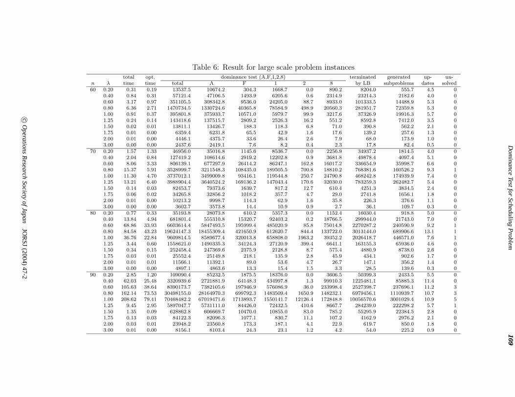
Finally, large scale problem instances are solved by the branch-and-bound algorithm withthe dominance test (A,F,1,2,8) with the Depth Parameter d = 0.5 and the root heuristics.For each pair of n and λ, 50 problem instances were generated. The result is shown in Tables6 and 5, where “opt. time” is the average time in seconds that an optimal schedule is foundand “unsolved” the average number of problem instances (out of 50) that cannot be solvedwithin 1800 seconds. Averages in these tables are taken from the solved problem instances.Since the average computational time of the solved problem instances is far less than 1800seconds, the problem instances may be classified into easy and quite hard. We have quitehard problem instances even with n = 70 and 80. A difference between “total time” and“opt. time” is the time spent to prove the optimality. Since much time is spent to provethe optimality, lower bounding computations and dominance tests should be improved todeal with large scale problem instances.

5. Concluding Remarks

In this paper, we considered the dominance test for a single machine scheduling problemwith release dates to minimize total flow time, based on the work of Chu [5]. We pointed outthat a naive combination of some dominance properties may lead to delete all of the optimalsolutions, and showed the way to avoid the pitfall by revising some dominance propertiesinto strict ones. Furthermore, new dominance properties were proposed though they wereineffective in our computational experiments. Chu [5] reported that the proposed branch-and-bound algorithm named BB C successfully solved problem instances with up to 100jobs. Though the computational environment has been improved since then, our proposed


Dom

inanceTestfor

SchedulingP

roblem109

Table 6: Result for large scale problem instancestotal opt. dominance test (A,F,1,2,8) terminated generated up- un-

n λ time time total A F 1 2 8 by LB subproblems dates solved60 0.20 0.31 0.19 13537.5 10674.2 304.3 1668.7 0.0 890.2 8204.0 555.7 4.5 0

0.40 0.84 0.31 57121.4 47106.5 1493.9 6205.6 0.6 2314.9 23214.3 2182.6 4.0 00.60 3.17 0.97 351105.5 308342.8 9536.0 24205.0 88.7 8933.0 101333.5 14488.9 5.3 00.80 6.36 2.71 1470734.5 1330724.6 40365.8 78584.9 498.9 20560.3 281951.7 72359.8 5.3 01.00 0.91 0.37 395801.8 375933.7 10571.0 5979.7 99.9 3217.6 37326.9 19916.3 5.7 01.25 0.24 0.14 143418.6 137515.7 2809.2 2526.3 16.2 551.2 8592.8 7412.0 3.5 01.50 0.02 0.01 13811.1 13426.7 188.3 118.3 6.8 71.0 390.8 562.2 2.1 01.75 0.01 0.00 6359.4 6231.8 65.5 42.9 1.6 17.6 139.2 257.6 1.3 02.00 0.01 0.00 4446.1 4375.7 33.6 26.4 2.6 7.9 68.0 173.9 1.0 03.00 0.00 0.00 2437.6 2419.1 7.6 8.2 0.4 2.3 17.8 82.4 0.5 0

70 0.20 1.57 1.33 46956.0 35016.8 1145.6 8536.7 0.0 2256.9 34937.2 1814.5 4.0 00.40 2.04 0.84 127419.2 108614.6 2919.2 12202.8 0.9 3681.8 49878.4 4097.4 5.1 00.60 8.06 3.33 806139.1 677297.9 26414.2 86247.1 162.8 16017.2 336654.9 35998.7 6.6 00.80 15.37 5.91 3528999.7 3211548.3 108435.0 189505.5 700.8 18810.2 768381.6 160526.2 9.3 11.00 11.30 4.70 3737012.1 3499009.8 93416.1 119544.8 250.7 24790.8 468242.8 174939.9 7.4 01.25 13.21 6.40 3988904.4 3640524.2 169136.2 147043.4 170.6 32030.0 783259.3 262482.7 5.4 01.50 0.14 0.03 82453.7 79373.6 1639.7 817.2 12.7 610.4 4251.3 3834.5 2.4 01.75 0.06 0.02 34265.8 32856.2 1018.2 357.7 4.7 29.0 2741.8 1656.1 1.8 02.00 0.01 0.00 10213.2 9998.7 114.3 62.9 1.6 35.8 226.3 376.6 1.1 03.00 0.00 0.00 3602.7 3573.8 14.4 10.9 0.9 2.7 36.1 109.7 0.3 0

80 0.20 0.77 0.33 35193.8 28073.8 610.2 5357.3 0.0 1152.4 16030.4 918.8 5.0 00.40 13.84 4.94 681801.4 555310.8 15320.7 92403.2 0.2 18766.5 299944.0 21743.0 7.0 00.60 68.86 33.93 6603614.4 5847493.5 195999.4 485020.9 85.8 75014.8 2270287.2 240590.9 9.2 10.80 84.58 43.23 19624147.3 18455309.4 421650.9 612620.7 844.4 133722.0 3013144.0 689906.6 13.1 11.00 36.76 22.84 9609814.5 8589677.4 320013.8 658808.0 1963.2 39352.2 2026418.7 446571.0 7.6 11.25 3.44 0.60 1558621.0 1490335.3 34124.3 27120.9 399.4 6641.1 163155.3 65936.0 4.6 01.50 0.34 0.15 252458.4 247369.6 2375.9 2128.8 8.7 575.4 4880.9 8738.0 2.6 01.75 0.03 0.01 25552.4 25149.8 218.1 135.9 2.8 45.9 434.1 902.6 1.7 02.00 0.01 0.01 11566.1 11392.1 89.0 53.6 4.7 26.7 147.1 356.2 1.4 03.00 0.00 0.00 4897.1 4863.6 13.3 15.4 1.5 3.3 28.5 139.6 0.3 0

90 0.20 2.85 1.20 109090.4 85232.5 1875.5 18376.0 0.0 3606.5 50399.3 2433.5 5.5 00.40 62.03 25.48 3320939.6 2721881.9 64148.3 434997.8 1.3 99910.3 1225481.1 85885.3 11.4 00.60 105.63 38.64 8390173.7 7382105.6 197946.9 576086.9 36.0 233998.4 2527398.7 237696.1 11.2 30.80 162.14 73.53 30498155.0 28164970.3 699792.3 1483509.4 1650.9 148232.1 6979456.1 1110939.7 10.7 31.00 208.62 79.41 70468482.2 67019471.6 1713893.7 1550141.7 12126.4 172848.8 10056570.6 3001029.4 10.9 51.25 9.45 2.95 5897047.7 5731111.0 84426.0 72432.5 410.6 8667.7 284239.0 222298.2 5.7 11.50 1.35 0.09 628862.8 606669.7 10470.0 10855.0 83.0 785.2 55295.9 22384.5 2.8 01.75 0.13 0.03 84122.3 82096.3 1077.1 830.7 11.1 107.2 4162.9 2976.2 2.1 02.00 0.03 0.01 23948.2 23560.8 173.3 187.1 4.1 22.9 619.7 850.0 1.8 03.00 0.01 0.00 8156.1 8103.4 24.3 23.1 1.2 4.2 54.0 225.2 0.9 0

c©O

perationsR

esearchSociety

ofJapanJO

RSJ

(2004)47-2

110S.Yanai&

T.Fujie

Table 7: Result for large scale problem instances (contd.)total opt. dominance test (A,F,1,2,8) terminated generated up- un-

n λ time time total A F 1 2 8 by LB subproblems dates solved100 0.20 3.48 1.53 136974.0 105464.9 1887.7 24980.3 0.0 4641.1 58765.7 2733.9 6.6 0

0.40 126.92 64.71 5365681.7 4280785.2 90150.7 861897.0 0.1 132848.8 2269907.1 130393.5 8.5 00.60 191.14 90.90 15475998.5 13064419.3 280093.5 1852240.9 1644.7 277600.1 4944087.3 409606.3 11.1 100.80 283.54 128.44 53271605.0 49222717.7 957637.1 2790066.8 3346.1 297837.3 9086021.3 1490558.5 11.2 81.00 147.81 42.38 47775044.7 45455974.5 1166193.6 877498.5 1711.9 273666.1 5418414.1 1594694.9 10.8 151.25 36.87 11.99 19612105.0 18905816.1 264517.1 361596.0 2572.0 77603.8 1202758.2 700344.0 6.5 21.50 1.45 0.61 775656.6 739728.6 18234.7 16442.9 564.0 686.3 71355.5 38798.7 3.5 01.75 0.18 0.05 160191.6 158195.0 1045.3 843.8 5.6 101.9 3361.9 5453.4 2.1 02.00 0.03 0.01 24820.9 24465.6 170.0 143.2 5.3 36.7 359.0 786.5 1.7 03.00 0.01 0.00 10112.9 10052.3 27.9 23.9 2.1 6.7 56.8 259.7 0.8 0

110 0.20 10.82 5.33 376458.7 292139.7 5587.6 64737.9 0.0 13993.4 160219.0 6657.2 7.5 00.40 205.30 101.39 8906038.2 7220911.3 144175.6 1316164.6 0.0 224786.6 3007994.7 174352.5 10.1 30.60 361.73 180.52 25408378.5 22359694.0 401989.0 2383674.5 210.0 262811.0 7379873.4 581622.1 14.3 170.80 412.12 185.47 73500592.7 66756257.0 1374318.0 4979849.2 1241.0 388927.4 15132465.0 2195539.2 11.9 201.00 305.76 83.60 112649972.5 107644263.8 1967400.5 2716676.8 13868.1 307763.2 11639149.4 3748471.5 10.1 191.25 33.00 16.68 19599772.4 18985041.4 218692.0 384639.7 2815.2 8584.0 1001533.3 646428.3 7.2 31.50 1.90 0.32 1313372.5 1278840.0 13080.7 20511.4 421.3 519.1 64801.5 51567.1 4.1 01.75 0.13 0.02 114753.1 112935.5 791.3 886.5 19.3 120.5 2299.8 3774.1 2.6 02.00 0.06 0.02 59073.3 58230.2 377.3 424.6 6.3 34.8 1088.1 2093.3 2.1 03.00 0.01 0.00 12216.8 12136.8 31.7 42.2 0.6 5.5 70.1 313.3 0.8 0

120 0.20 40.35 17.73 1247747.6 923130.0 15019.3 250208.8 0.0 59389.4 527621.5 20498.0 8.1 00.40 274.65 138.91 9594414.6 7820240.2 113102.8 1488076.9 0.0 172994.7 3773522.3 185977.3 13.4 150.60 435.18 90.33 32058010.5 27990498.1 478598.5 2961442.4 324.6 627146.8 7163372.8 609708.9 15.1 330.80 423.70 193.83 68613594.5 63414285.7 985198.4 3898956.1 1478.7 313675.5 14717966.8 1757496.8 11.2 391.00 368.47 123.41 156302410.0 150093230.5 2549304.1 3273660.4 24445.7 361769.3 13292652.9 4430534.5 13.0 341.25 95.00 41.23 68806510.0 67566700.6 640364.6 457149.3 2590.6 139704.9 1777436.0 1908890.2 6.4 81.50 25.62 0.64 23155942.5 22844369.7 172352.5 132202.4 253.5 6764.5 519166.6 604830.6 3.2 01.75 1.07 0.25 987962.2 975914.3 6218.2 5295.3 22.9 511.7 15937.6 26707.5 2.6 02.00 0.10 0.02 92021.9 90950.8 608.9 373.1 7.4 81.6 1210.5 2492.2 1.7 03.00 0.02 0.01 17720.5 17627.0 42.0 42.3 2.0 7.3 91.2 398.1 0.9 0

c©O

perationsR

esearchSociety

ofJapanJO

RSJ

(2004)47-2


branch-and-bound algorithm with the dominance test (A,F,1,2,8) with the Depth Parameterd = 0.5 cannot outperform BB C. Moreover, as was pointed out in Section 4.2, the branch-and-bound algorithm with incorrect dominance test may run slower than the algorithm withthe corresponding correct dominance test. Since detailed description of BB C (especially adesign of the dominance test used in BB C) is not provided in [5], our result may be a truelimit of branch-and-bound algorithms using the lower bounding computation based on theSRPT rule and the dominance properties introduced in Section 3.

Acknowledgements

The authors would like to thank Professors Kensaku Kikuta, Toshio Hamada and TeruhikoYoshida for their helpful comments and suggestions. Thanks are also due to the anonymousreferees for many valuable comments.

References

[1] R. H. Ahmadi and U. Bagchi: Lower bounds for single-machine scheduling problems.Naval Research Logistics, 37 (1990), 967–979.

[2] K. R. Baker: Introduction to Sequencing and Scheduling (Wiley, New York, 1974).

[3] P. Baptiste, C. Le Pape and W. Nuijten: Constraint-Based Scheduling – Applying Con-straint Programming to Scheduling Problems (Kluwer Academic Publishers, Boston,2001).

[4] L. Bianco and S. Ricciardelli: Scheduling of a single machine to minimize total weightedcompletion time subject to release dates. Naval Research Logistics Quarterly, 29 (1982),151–167.

[5] C. Chu: A branch-and-bound algorithm to minimize total flow time with unequal releasedates. Naval Research Logistics, 39 (1992), 859–875.

[6] M. I. Dessouly and J. S. Deogun: Sequencing jobs with unequal ready times to minimizemean flow time. SIAM Journal on Computing, 10 (1982), 192–202.

[7] A. M. A. Hariri and C. N. Potts: An algorithm for single machine sequencing withrelease dates to minimize total weighted completion time. Discrete Applied Mathematics,5 (1983), 99–109.

[8] T. Ibaraki: The power of dominance relations in branch-and-bound algorithms. Journalof the Association of Computing Machinery, 24 (1977), 264–279.

[9] W. H. Kohler and K. Steiglitz: Characterization and theoretical comparison of branch-and-bound algorithms for permutation problems. Journal of the Association of Comput-ing Machinery, 21 (1974), 140–156.

[10] J. K. Lenstra, A. H. R. Rinnooy Kan and P. Brucker: Complexity of machine schedulingproblems. Annals of Discrete Mathematics, 1 (1982), 343–362.

Shuzo YanaiGraduate School of Business AdministrationKobe University of Commerce8-2-1 Gakuen-nishimachi, Nishiku,Kobe 651-2197, JAPANE-mail: [email protected]


Documents

ON A DOMINANCE TEST FOR THE SINGLE MACHINE …archive/pdf/e_mag/Vol.47_02_096.pdf · ON A DOMINANCE TEST FOR THE SINGLE MACHINE SCHEDULING ... Branch-and-bound algorithm is a fundamental