"SINGLE MACHINE SCHEDULING TOMINIMIZE TOTAL WEIGHTED

LATE WORK"

by

A.M.A. HARIRI,*C.N. POTTS**

andLuk VAN WASSENHOVE***

N° 92/29/TM

* Department of Statistics, King Abdul-Aziz University, Jeddah,Saudi Arabia.

* * Faculty of Mathematical Studies, University of Southampton, Southampton, England.

*** Professor of Operations Management and Operations Research, INSEAD, Boulevard de Constance,Fontainebleau 77305 Cedex, France.

Printed at INSEAD,Fontainebleau, France

SINGLE MACHINE SCHEDULING TO

MINIMIZE TOTAL WEIGHTED

LATE WORK

A.M.A. Hariri

Department of Statistics, King Abdul-Aziz University, Jeddah, Saudi Arabia

C.N. Potts

Faculty of Mathematical Studies, University of Southampton, U.K.

L.N. Van Wassenhove

INSEAD, Fontainebleau, France

In the problem of scheduling a single machine to minimize total weighted latework, there are n jobs to be processed for which each has an integer processing

time, a weight and a due date. The objective is to minimize the total weightedlate work, where the late work for a job is the amount of processing of this job

which is performed after its due date. An 0(n log n) algorithm is derived for the

preemptive total weighted late work problem. For non-preemptive scheduling, ef-

ficient algorithms are derived for the special cases in which all processing times

are equal and in which all due dates are equal. A pseudopolynomial algorithm ispresented for the general non-preemptive total weighted late work problem. Also, a

branch and bound algorithm in which lower bounds are obtained using the dynamic

programming state-space relaxation method is proposed for this general problem.

Computational results with the branch and bound algorithm for problems with upto 700 jobs are given.

Subject classification: Scheduling: single machine, weighted late work, branch and

bound algorithm.

The problem of scheduling a single machine to minimize total weighted latework may be stated as follows. Each of n jobs (numbered 1, , n) is to be processedon a single machine which can handle only one job at a time. Job i (i = 1, , n)becomes available for processing at time zero, requires a positive integer processingtime pi , has a positive weight tvi and has a positive integer due date d,. In thepreemptive version of this problem, processing may be interrupted and resumed ata later time, but in the non-preemptive problem no interruption in the processingof a job is allowed. We assume that jobs are numbered in non-decreasing order oftheir due dates (EDD order) so that d1 < < da, and to; > tvi4. 1 if di = d,+1(i = 1, , n – 1). Given a schedule a that defines the completion time Ci (a) ofjob i (i = 1, , n), the late work Vi(o) for job i, which is the amount of processingperformed on i after its due date, is easily computed. When no ambiguity results,we abbreviate Ci(a) and Vi(a) to Ci and V; respectively. If V, = 0, then job i isearly; if 0 < V, < pi , then job i is partially early; alternatively, if V. = p i , then job iis late. We refer to pi – Vi as the early work for job 1. The objective is to schedulethe jobs so that the total weighted late work E7 w,V, is minimized.

Problems which involve the scheduling of jobs with due dates on a single ma-chine to minimize total cost have been widely studied in the literature. Two of theseare related to the non-preemptive total weighted late work problem. Firstly, in thetotal weighted tardiness problem, which is (unary) NP-hard (Lawler [7], Lenstra etal. [9]), the cost of scheduling job i (i = 1, , n) to be completed at time Ci is givenby its weighted tardiness w; T; = w, max{Ci – d„ 0}. Clearly, w i lt, = wi min{ T„p,}for non-preemptive scheduling. An effective branch and bound algorithm whichsolves total weighted tardiness problems with up to 40 jobs is given by Potts andVan Wassenhove [10]. Secondly, in the weighted number of late jobs problem, thecost associated wish job i is wi ll„ where U, = 1 if C, > di and U, = 0 otherwise.A pseudopolynomial dynamic programming algorithm for this (binary) NP-hardproblem (Karp [5]) is given by Lawler and Moore [8]. Potts and Van Wassenhove[11] present dynamic programming and branch and bound algorithms which solveweighted number of late jobs problems with up to 1000 jobs.

The total weighted late work problem is first studied by Blazewicz [2]. Heshows that the problem of preemptively scheduling jobs with release dates on iden-tical parallel machines can be solved using linear programming and is hence poly-nomially solvable. Potts and Van Wassenhove [12] derive an 0(n log n) algorithmfor the preemptive single machine problem with unit weights. They also show thatthe corresponding non-preemptive problem is (binary) NP-hard and they derive apseudopolynomial dynamic programming algorithm which enables problems withup to 10 000 jobs to be solved.

The total weighted late work problem has applications in information pro-cessing. In this context, a job is a message carrying an amount of informationproportional to its length. All information received after a given due date is uselessand is referred to as information loss. Total weighted information loss is minimizedby solving a total weighted late work problem. More generally, applications occurin any situation that involves a perishable commodity which deteriorates after agiven due date.

1

This paper derives algorithms for the preemptive and non-preemptive totalweighted late work problems. The remaining sections are organized as follows. Sec-tion 1 derives an O(n log n) algorithm for the preemptive problem, while subsequentsections deal with non-preemptive scheduling. Some special cases for which poly-nomial time algorithms are available are analyzed in Section 2. In Section 3, afterderiving a key result on the structure of an optimal sequence, a pseudopolynomialdynamic programming algorithm is given. Subsequent sections of the paper are de-voted to the derivation and computational testing of a branch and bound algorithm.Section 4 uses the recursion of Section 3 to derive, through the application of thedynamic programming state-space relaxation technique, a lower bounding scheme.Also included is the description of a heuristic which uses dynamic programming togenerate an upper bound. Reduction tests, whereby jobs are discarded from theproblem because they are either necessarily early or necessarily late, are given inSection 5. Section 6 analyzes various structural properties of the problem whichenable the lower bounding scheme to be implemented more efficiently. Full detailsof our branch and bound algorithm are given in Section 7. Section 8 reports on com-putational experience with the algorithm and some concluding remarks are givenin Section 9.

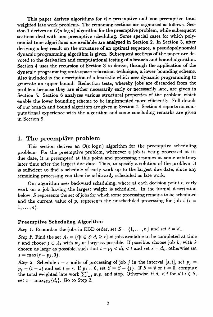
1. The preemptive problemThis section derives an O(n log n) algorithm for the preemptive scheduling

problem. For the preemptive problem, whenever a job is being processed at itsdue date, it is preempted at this point and processing resumes at some arbitrarylater time after the largest due date. Thus, to specify a solution of the problem, itis sufficient to find a. schedule of early work up to the largest due date, since anyremaining processing can then be arbitrarily scheduled as late work.

Our algorithm uses backward scheduling, where at each decision point t, earlywork on a job having the largest weight is scheduled. In the formal descriptionbelow, S represents the set of jobs for which some processing remains to be scheduledand the current value of p, represents the unscheduled processing for job i (i =1, , n).

Preemptive Scheduling Algorithm

Step I. Renumber the jobs in EDD order, set S = {1, , n} and set t =

Step 2. Find the set A t = {ili E S; d, > t} of jobs available to be completed at timet and choose j E A i with w3 as large as possible. If possible, choose job k, with kchosen as large as possible, such that t — pi < dk < t and set s = dk ; otherwise sets = max{t —p„0}.

Step 3. Schedule t - s units of processing of job j in the interval [s, t], set pi =pi — (t - s) and set t = s. If pi = 0, set S = S - {j}. If S = 0 or t = 0, computethe total weighted late work E: 1 1 to,p, and stop. Otherwise, if d, < t for all i E S,set t = max, E dd,}. Go to Step 2.

2

We claim that the Preemptive Scheduling Algorithm generates at most n pre-emptions. To justify our claim, we note that a preemption occurs when less thanp3 units of processing of job j are scheduled in Step 3. This occurs either whent –pi <dk <t for some k (k = 1, ,n –1) or when t –pi < 0 < t; thus, our claimis established. If desired, the number of preemptions may be reduced to at mostn – 1 by rescheduling all early work in EDD order and eliminating any preemptionat time 4 by appropriate scheduling of late work to start at time 4.

Since at most n preemptions are generated by the Preemptive Scheduling Algo-rithm, Steps 2 and 3 of the algorithm are executed at most 2n times. It is apparent,therefore, that the algorithm requires 0(n log n) time. Note also that the Preemp-tive Scheduling Algorithm remains valid if processing times and due dates becomearbitrary positive real numbers.

Lastly in this section, we prove that the algorithm generates an optimal solu-tion.

Theorem 1. The schedule generated by the Preemptive Scheduling Algorithmminimizes the total weighted late work.

Proof. Consider an optimal schedule r* and compare it with a schedule 70 gener-ated by the Preemptive Scheduling Algorithm. We assume that in 71-", any process-ing scheduled before time 4 is early work; otherwise it can be rescheduled aftertime 4 without affecting the total late work. It is also assumed that r* has afinite number of preemptions: we observe that an optimal schedule obtained fromthe linear programming algorithm of Blazewicz has this property. We show that afinite sequence of transformations of ir", each of which does not increase the totalweighted late work, yields the schedule 7rA.

Suppose that r* and Ir A are not identical in the time interval [0,4]. Let tbe chosen as small as possible so that these schedules are identical in the interval[t, dn ]. In 7r A , suppose that processing on job j is scheduled in the interval [s, t]and not processed immediately before time s. (The machine cannot be idle justbefore time t in the schedule ir A because if it were, the mechanics of the PreemptiveScheduling Algorithm ensure that no early work is available, so the machine wouldalso be idle in ir` immediately before time t, thereby contradicting the definitionof t.) Consider first the case that in 7r*, the machine is idle in the interval [r, t],but is not idle immediately before time r. Let q = max{r,s}. We transform e bymoving t – q units of processing of job j into the interval [q, t], where this processingis originally scheduled before time q or after time 4. Since the processing movedinto [q, t] is completed by time di (the Preemptive Scheduling Algorithm would notschedule job j in the interval (s, t] otherwise), this transformation does not increasethe total weighted late work. We now consider the alternative case that in 7r*, job i(i j) is processed in the interval {r, t) and not processed immediately before timer. We transform by interchanging the t – q units of processing of job i scheduledin [q, t] with t – q units of processing of job j which are originally scheduled beforetime q or after time 4. Since, in the Preemptive Scheduling Algorithm, jobs i and

3

j are candidates for scheduling immediately before time t, job j is selected because> w,. Any interchange of processing of job i with early work for job j (scheduled

before time q) leaves the total weighted late work unaltered. Furthermore, anyinterchange of processing of job i with processing which corresponds to late workfor job j decreases the total weighted late work by w i - wi per unit of interchange.Thus, this transformation does not increase the total weighted late work either. Inboth cases, the transformed schedule, which is also optimal, is identical with j.A

in the interval [q, d,,]. Since rr" and r A each have a finite number of preemptions,repetition of this argument shows that an optimal schedule rt it is obtained after afinite number of transformations of r*. q

2. Special casesHenceforth, we consider non-preemptive scheduling. In this section, we present

an 0(n) algorithm for the case of identical due dates and an 0(n 3 ) algorithm forthe case of identical processing times.

We consider first the case of identical due dates for which d, = d for i = 1, , n,where d is a positive integer. We assume that d < p,; otherwise, any sequenceis optimal. Recall that jobs with equal due dates are numbered in non-increasingorder of weights. Thus, w i > > w,,. The following result provides a class ofoptimal sequences.

Theorem 2. For the case of identical due dates, if j is chosen so that Eji: p, <d < El., p i , then any sequence in which jobs 1,..., j - 1 are scheduled before jobj and jobs j + 1, , n are scheduled after job j is optimal.

Proof. Suppose that the Preemptive Scheduling Algorithm is applied. It schedulesall the processing of jobs 1,... ,j - 1 and d - E;7: p, units of processing of jobj as early work. By scheduling jobs 1, , j - 1 (in any order) in the interval[0, E .:: 11 and then the early work for job j in the interval we stillhave an optimal preemptive schedule. A non-preemptive schedule is obtained byappending any late work for job j, followed by jobs j +1, , n (in any order). Sincethis non-preemptive schedule has the same total weighted late work as the optimalpreemptive schedule, it is an optimal non-preemptive schedule. q

To complete our analysis of the case of identical due dates, we show thatjob j of Theorem 2 can be found (without renumbering the jobs) in 0(n) time.We assume that all weights are distinct: this can be achieved, if necessary, byperturbing the weights. Let w, be the median weight which is found in 0(n) time(Blum et al. [3], Schonhage et al. [13]). Also, let A- = {hlw h < wi }, A = {i} andA+ = {hlw h > w,}. Either EhEA+ p h > d in which case the search for job j isrestricted to A+ while the jobs of A- and A are late; or EhEA - Ph > EA-1 ph - din which case the search for job j is restricted to A- while the jobs of A and A + areearly; or EhEA + Ph < d < Eh=1 Ph - EhEA - ph in which case the search ends with

4

j i while the jobs of A + are early and the jobs of A" are late. To continue thesearch in the former cases, late jobs are discarded immediately, whereas early jobsare discarded after their processing times are subtracted from d. Furthermore, thesearch for job j is restricted to a subset containing at most n/2 jobs. Reapplying theprocedure requires one half of the time required by the first application and restrictsthe search to a subset containing at most n/4 jobs. After O(log n) applications ofthe procedure which are carried out over subsets which contain at most n, n/2, n/4,... jobs, job j is found in 0(n) time. It is now clear from Theorem 2 that the caseof identical due dates is solvable in 0(n) time.

We consider now the case of identical processing times for which pi p fori = 1, , n, where p is a positive integer. If job i (i = 1, , n) is sequenced inposition j (j = 1, ... , n), then it has completion time jp from which its weightedlate work is given by

c,) = wi min { max {jp — d,, 0} , p, .

It is now apparent that, using the algorithm of Lawler 161, an optimal sequence maybe found in 0(n 3 ) time from the solution of a linear assignment problem with costsc11 . Thus, the case of equal processing times is solvable in 0(n3 ) time.

3. A dynamic programming algorithmHenceforth, the general problem of non-preemptively scheduling jobs on a single

machine to minimize the total weighted late work is considered. In this section,we derive a pseudopolynomial dynamic programming algorithm for this problem.The algorithm relies on the closeness of an optimal schedule of early and partiallyearly jobs to an EDD sequence; this issue is discussed first. Consider the followinginstance. There are two jobs for which m = 3, w1 = 1, d1 = 5, m = 4, w 2 = 3 andd2 = 6. The total weighted late work for the sequence (2,1) is 2, which is less thanthe value of 3 that is given by EDD sequence (1, 2). Thus, in contrast to the totallate work problem where w i = 1 (i = 1, ,n), we cannot assume that early andpartially early jobs are sequenced in EDD order.

Clearly, an optimal schedule is specified by a sequence of early and partiallyearly jobs which we call a non-late sequence; any late jobs can be appended to thissequence in an arbitrary order. Job i is deferred (from its EDD position) in a non-late sequence a if it is sequenced after a job having a due date larger than d,. If jobi is sequenced immediately after job j in a, where d, > di , then ji forms a reversedpair in a.

The following result establishes the ordering of jobs with the same due date inan optimal non-late sequence a. It also shows we may assume that jobs of a arealmost in EDD order in the sense that for each job j of a, at most one job with asmaller due date is sequenced after it.

Theorem 3. There exists an optimal non-late sequence a such that jobs of a withthe same due date are sequenced in non-increasing order of their weights and, for

5

each job j of a, at most one job having a due date smaller than d1 appears after jin a.

Proof. Let a be any optimal non-late sequence. We show that a finite sequence oftransformations of a, each of which does not increase the total weighted late work,yields an optimal non-late sequence which satisfies the conditions of the theorem.Suppose that a does not satisfy the conditions of the theorem. We consider firstthe case that some job j is sequenced before job i in a, where d, = di and w, > w1.It is apparent that job j is early in a since if it were partially early, then job iwould be late. Firstly, suppose that Vi(a) > p,. Consider the effect of removingjob j from a so that it is deemed to be late. The weighted late work for job idecreases by w ipi to give a decrease in the total weighted late work of at leastpi (wi – wi ) > 0. However, this contradicts the choice of a as an optimal non-latesequence. Therefore, 0 < Vs (a) < p„. Consider now the non-late sequence a' whichis obtained from a by removing job j from its original position and inserting itimmediately after job i. Clearly, V1 (a') = 0 and V„(a') = Vi (a). Furthermore, onlyjob j has a later completion time in a' than in a. Thus, we deduce that

w,V,(a) w,V,(a)– w,V,(a') – w„V„(a 1 ). (wi – w„)V,(cr) 0

which shows that a' is an alternative optimal non-late sequence. By repeating thisargument, an optimal non-late sequence results in which jobs having the same duedate are sequenced in non-increasing order of their weights.

Alternatively, suppose that a is an optimal non-late sequence in which jobshaving the same due date are sequenced in non-increasing order of their weights,but does not satisfy the conditions of the theorem. Choose the last job j of a whichis sequenced before jobs i and i', where d, < d, and di, < di . We assume withoutloss of generality that job i is sequenced before job i' in a. From the inequalityCi(a) < de, which is valid since otherwise job i' would be late in a, we deducethat C1 (a) < d„. Consider now the non-late sequence a' which is obtained froma by removing job j from its original position and inserting it immediately afterjob i. We observe that C,(a') = C,(a) < d„. Since no job is completed later ina' than in a except job j which has zero late work in a and a', it is clear that a'is also an optimal non-late sequence. Furthermore, a' also has the property thatjobs with the same due date are sequenced in non-increasing order of their weights.By repeating this argument, an optimal sequence satisfying the conditions of thetheorem is obtained after a finite sequence of transformations of a.

We now proceed with the derivation of our pseudopolynomial dynamic pro-gramming algorithm. It generalizes the algorithms of Lawler and Moore for theproblem of minimizing the weighted number of late jobs and of Potts and VanWassenhove [121 for the total late work problem.

We first show how Theorem 3 allows us to perform a structured search foran optimal non-late sequence. We restrict our search to EDD-maximal non-latesequences for which the interchange of jobs j and i in any reversed pair ji results in

6

an increase in the total weighted late work. Note that if ji is a reversed pair in anEDD-maximal non-late sequence o, then job j is early and job i is partially early.To justify this assertion, we observe that if job j is completed after time di , thendi > di shows job i to be late and hence not in a; thus, job j is early. Furthermore, ifjob i is early, then jobs j and i remain early if they are interchanged which impliesthat a is not EDD-maximal; thus, job i is partially early. Thus, if job i of thereversed pair ji is completed at time t, then i E where

Air = {iId;< di;d,<t<d; + p;;i= 1,...,j- 1}.

In our structured search, jobs are considered in natural (EDD) order 1, , n.Job i can either be declared late, be declared early or partially early and not de-ferred, or be deferred. Suppose that job i is deferred to be sequenced immediatelyafter job j, where di > di and consequently j > i. Theorem 3 ensures that all non-late jobs amongst i + 1,...,j are sequenced in their natural order. Thus, at anystage of the procedure, there is at most one job which is deferred, but not currentlysequenced.

Our dynamic programming algorithm utilizes this search procedure. In addi-tion to the variable j which indicates that jobs 1,...,j only are considered, thealgorithm uses a state-space that consists of (t, i). The last element specifies whichjob, if any, is deferred: if i = 0, there is no deferred job; however i E {1, , j}indicates that job i is deferred and will be sequenced immediately after one ofthe jobs j + 1, ,n. Also, t represents the time at which non-late jobs amongst{1, , j} - {i} are completed. The dynamic programming recursion is definedon values fi (t, i) which represent the minimum total weighted late work for jobs1,.. . , j when non-late jobs amongst {1, j - {i} are completed at time t, whereany deferred job i contributes wip, in the computation of fi (t, i). (An equivalent al-gorithm can be derived in which a deferred job i has a zero contribution in fi (t, i).)Thus, for each j (j = 1, , n), fi (t,i) is defined for t = 0, ... ,Ti and i = 0, , j,where Ti = ph.

Our recursion equations are:

min{ fi_ i (t, 0) + tv;p;, fi- i (t - pi , 0)+wimax{t - di , 0},mini E Ap{fi- 1 (t -pi - pi , i)

fi (t, 0) = +tvi(t - - pi )} } for t < di +Pi,

min { fi _ i (t, 0) + {fi-i (t - p; - pi , i)- di - pi ))) for t > di + pi;

{ min{ fi_ i (t, + wipi , fi_ (t - pi , 0} for t < di,fi(t, = (i = 1,...,j -1)

co for t > di;

fi_ i (t, 0) + wipi for t <

oo for t > di;

where /0 (0, 0) = 0 and all other initial values are set to infinity.

7

Some explanation of these recursion equations is appropriate. In the compu-tation of fi (t, 0) for t < di + pi , the three terms in the minimization correspondto the decisions that job j i s late, job j is scheduled in the interval [t – t] to benon-late, and job j and the deferred job i are sequenced successively in the interval[t –pi – pi , t]. In the latter case, the definition of Ali ensures that job j is early andjob i is partially early, while the weighted late work tv i(t – di ) of job i is added andthe contribution w,p, assumed in (t – p, i) is subtracted from the functionvalue. When t > di + pi , the computation is similar except that the second term,which assumes that job j is non-late when completed at time t, is deleted. Forf,(t, i), which is defined for t < ds since otherwise job i must be late, the casesthat job j is late or is early are considered (job j cannot be partially early whencompleted at time t since t < < di ). Finally, the computation of Mt, j), whichis defined for t < di since otherwise job j must be late, sets job j to be deferred.

The recursion equations for fi (t,i) are solved for j = 1, , n, t = 0, , 7", andi = 0, ,j after which min=.-.0,...,T„ {f.(t,0)} provides the minimum total weightedlate work. Since lAid < n, our dynamic programming algorithm requires 0(712 T„ )time. This establishes that the total weighted late work problem is pseudopolyno-mially solvable because T. = Eh. 1 ph.

In Sections 5 and 6, various devices are presented which help to reduce the timeand storage requirements of the dynamic programming algorithm. Even with thesedevices, however, the algorithm is awkward to implement and storage requirementsare substantial. As an alternative, we propose a branch and bound algorithm inwhich the lower bounds are derived, using the dynamic programming state-spacerelaxation method, from the recursion given above. The remainder of the paper isdevoted to a description and an evaluation of our branch and bound algorithm.

4. Lower and upper boundsIn this section, dynamic programming is used to establish lower and upper

bounds on the minimum total weighted late work; these bounds are used in ourbranch and bound algorithm. Firstly, we derive a lower bounding scheme by ap-plying the dynamic programming state-space relaxation method to the recursionof the previous section. Dynamic programming state-space relaxation is a tech-nique proposed by Christofides et al. [4] for routing problems and is developed byAbdul-Razaq and Potts [1] for single machine scheduling. The method maps thestate-space of a dynamic programming recursion onto a smaller state-space andcomputes a lower bound by performing the recursion on the smaller state-space.

In addition to the state variable j, the recursion of the previous section usesa state-space consisting of (t, i), where the value of i defines any deferred job. Werelax this state-space by mapping (t, i) onto t, i.e., the mapping discards the statevariable defining any deferred job.

Our relaxed dynamic programming recursion is defined on values f;(t). To en-sure that a valid lower bound is obtained, we require that f;(t) < {f7(t, i)}.

8

By defining

min{ f.;_ i (t) + wiPi, 4- 1 ( t - Pi) + wj max{t - di , 0},mini€A;,{4- 1 ( t -Pj — PO+ wi(t - di - PO)} for t < di + Pi,

f(t)=min {4_ 1 (t) + wjpi , miniEAp tri—i(t — Pi — Pi)

1-tvi(t - di - p i )} for t > di + pi,

where MO) = 0 and all other initial values are set to infinity, a straightforwardinductive argument shows that this requirement is satisfied. We note that in thecomputation of 4(0, decisions may be taken to schedule a job twice, the first timein its EDD position and the second time as a deferred job.

The recursion equations for f (t) are solved for j = 1, ...,n and t = 0, ...after which the lower bound is computed using LB = {f,;(t)}. Thecomputation of the lower bound requires 0(n2T„) time. A backtracking procedureyields the corresponding non-late 'sequence'. If this 'sequence' contains no repeatedjob, then it is optimal. Otherwise, the branch and bound algorithm described inSection 7 is applied.

Included in Section 6 is the derivation of a procedure that allows jobs to beeliminated from Aii . Results of initial experiments show I to be very small forall j and t, after this procedure is applied. Therefore, for practical purposes, ourrecursion for computing lower bounds resembles an 0( nT„) procedure, and is moreefficient than the 0(12 2 2,,) dynamic programming algorithm of Section 3.

The following dynamic programming heuristic is applied at the root node ofthe search tree in our branch and bound algorithm. Our heuristic computes anoptimal solution to the problem in which deferred jobs are not allowed, i.e., earlyand partially early jobs are constrained to be sequenced in EDD order. Let gj(i)denote the minimum total weighted late work incurred when scheduling jobs 1, . . . , jso that early and partially early jobs are sequenced in EDD order and the last ofthese non-late jobs is completed at time t. From the equations of Section 3 for

(t , 0), we obtain the following recursion:

minfg) _ 1 (t) wipi ,Y j-i(t - Pi)g i(t) = max{t - dj , On for t < di + pj

gj_ i (t)+ wipifor t>di+ Pi

where go(0) = 0 and all other initial values are set to infinity. After computinggj (t) for j = 1, , n and t = 0, , Ti , we obtain UB = {gn(t)} as theweighted late work for our approximate solution. Clearly, this heuristic requires0(nT,,) time. The substantial computational requirements are partly justified bythe results of initial experiments which show that the the heuristic generates anoptimal solution in many cases.

The two following sections present various devices which help to improve theeffectiveness of our branch and bound algorithm. Section 5 describes reductiontests whereby jobs can be discarded from the problem. Also, we give a redundant

9

state elimination procedure which allows the recursions of this section to be solvedmore efficiently. In Section 6, we derive a reversed pair elimination procedure whichrestricts the cardinality of the sets Alt : in addition to reducing the computationtime for LB, there is a decreased likelihood that the 'sequence' corresponding to LBcontains repeated jobs and consequently the lower bound becomes tighter.

5. Reduction tests

.5.1 Earliness testFor our earliness test, we establish conditions whereby jobs can be removed

from the problem because they are necessarily early when sequenced after all otherearly and partially early jobs. Specifically, we aim to show, for some index j, thatjobs j + 1, , n are early in at least one optimal schedule; we choose j as smallas possible, subject to the conditions of the test. For the problem involving jobs1, ,i only (i = 1, , n), we define recursively the latest completion time 7;1' ofthe last early or partially early job using

= min{ T81' + p i , max {d h + ph — 1} } , (1)

where To = 0. (A justification for the use of this recursion is given below in theproof of Theorem 4.) If jobs j + 1, , n are necessarily early when sequenced inEDD order after the last early or partially early job amongst 1,... , j, then clearlyj + 1, ...,n are early in at least one optimal schedule. The earliness test selects jas small as possible, subject to

TL + E ph < dh for k j 1, . . . , n, (2)h=i+i

and discards jobs j + 1, , n from the problem. We show next that an optimalsolution is obtained by appending jobs j + 1, , n to an optimal non-late sequencefor the reduced problem.

Theorem 4. An optimal solution is obtained by applying the earliness test, solvingthe reduced problem, and then inserting jobs j + 1, , n immediately after the lastearly or partially early job of the optimal sequence for the reduced problem.

Proof. If the last early or partially early job of the reduced problem is completedby time Tj1', then clearly (2) allows jobs j +1, ,n to be inserted without increasingthe total weighted late work. Thus, it is sufficient to show that the last early orpartially early job amongst 1, ,j is completed not later than time TL.

We consider three cases. Firstly, if TL = ELI p„ then it is clear that jobs1, . . . , j are completed by time TL . Secondly, if 71 = {d, + p, — 1}, then

10

any of the jobs 1,... , j is late if it is completed after time Tfr. Finally, suppose thatTL = 11111.Xy=1,...,i{dh + Ph + Ei=i+i ph for some job i (i = 1, , j — 1). Thelast early or partially early job amongst 1, ,i is completed not later than timemaxh=1,...,i + ph —1). Furthermore, after this last job is completed, a maximumof Els.i+1 ph additional units of processing are required to complete any furtherearly or partially early jobs amongst 1, . , j. Thus, the desired result holds for allthree cases. q

5.2 Latene.s3 teatOur lateness test gives conditions under which jobs can be removed from the

problem because they are necessarily late in any optimal schedule. Let LB ) bea lower bound on the total weighted late work when job j is constrained to beearly or partially early. (The computation of LB ) using the Preemptive SchedulingAlgorithm is explained below.) If LB j > UB, where UB is obtained by applying ourdynamic programming heuristic of Section 4 (although any other upper bound onthe total weighted late work can be used), then in any optimal schedule job j mustbe late. Thus, after the evaluation of its contribution wjp, to the total weightedlate work, job j is discarded to give a reduced problem. The test is applied for eachjob j except those which, in the solution generated by the Preemptive SchedulingAlgorithm applied to the original problem, are early.

The computation of the lower bound LB j using the Preemptive SchedulingAlgorithm is described now. Since job j is constrained to be early or partially early,it must be completed no later than time di + pi — 1. To enforce this constraint,we assign a large weight to job j and reset its due date to d1 + pi — 1. The valueLBj is the minimum total weighted late work for the preemptive problem havingprocessing times pi, = pi (i = 1, ... ,n), weights w: = w i (i = 1, , n; i j) and

= oo, and due dates d: = d, (i = 1, , n; i j) and di = + — 1.The following results justifies the use of our lateness test.

Theorem 5. An optimal solution is obtained by applying the lateness test toeliminate some set L of jobs, solving the reduced problem, and then appending thejobs of L to the optimal sequence for the reduced problem.

Proof. For a fixed job j, it is sufficient to establish that LB, is a valid lower boundon the total weighted late work for the (non-preemptive) constrained problem. Let7r denote an optimal sequence for this problem which defines 1/,(7r) as the latework for job i (i 1, , n). Suppose that 7t is evaluated with respect to thedata for the preemptive problem to give Vi1 (7r) as the late work for each job i.Clearly, Vii (7r) = V,(77) for i = 1, , n and i j. Since by the constraint on jobj we have Ci(7r) < di + pi — 1, it follows that 171(7r) = 0 < 17) (4 Therefore,

tv 1 V;(7r) > wiVis(7r) > LBj , where the final inequality holds becauseLBj is the minimum total weighted late work for the preemptive problem. It is nowapparent that LBj is a valid lower bound for use in our lateness test. q

11

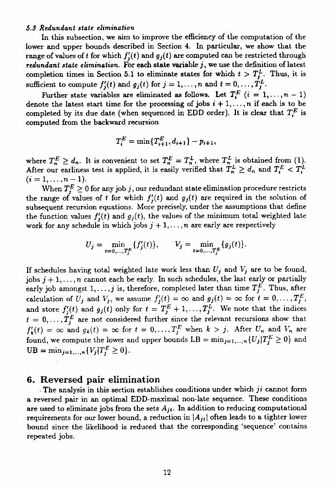
5.5 Redundant state eliminationIn this subsection, we aim to improve the efficiency of the computation of the

lower and upper bounds described in Section 4. In particular, we show that therange of values of t for which f;(t) and 9) (0 are computed can be restricted throughredundant state elimination. For each state variable j, we use the definition of latestcompletion times in Section 5.1 to eliminate states for which t > 71'. Thus, it issufficient to compute ry (t) and g,(t) for j = 1, , n and t = 0, ...

Further state variables are eliminated as follows. Let TT (i = 1, , n — 1)denote the latest start time for the processing of jobs i + 1, ,n if each is to becompleted by its due date (when sequenced in EDD order). It is clear that TiE iscomputed from the backward recursion

T,E = min{T,E+ 1 ,d1+1} — P.+1,

where Tn > dn . It is convenient to set Tif = Trf', where 7',.f is obtained from (1).After our earliness test is applied, it is easily verified that Trf > do and T,E < T,L(i = 1,...,n — 1).

When > 0 for any job j, our redundant state elimination procedure restricts)the range of values of t for which f",(t) and g,(t) are required in the solution ofsubsequent recursion equations. More precisely, under the assumptions that definethe function values j",(t) and g,(t), the values of the minimum total weighted latework for any schedule in which jobs j n are early are respectively

U, = min ff:(t)), V, = min {MO).t= 0

If schedules having total weighted late work less than U, and V1 are to be found,jobs j 1, ,n cannot each be early. In such schedules, the last early or partiallyearly job amongst 1,...,j is, therefore, completed later than time Tr. Thus, aftercalculation of U, and V3 , we assume fl (t) = a) and g,(t) = oo for t 0, ,and store f_7 (t) and gl (t) only for t = TE + 1, We note that the indicest = 0, , TjE are not considered further since the relevant recursions show that

fl( t ) = co and g k (t) oo for t = 0, , Tr when k > j. After Un and 17„ arefound, we compute the lower and upper bounds LB = min3. 1 ..... .{U3 IT3E > 0) andUB = > 0}.

6. Reversed pair elimination- The analysis in this section establishes conditions under which ji cannot form

a reversed pair in an optimal EDD-maximal non-late sequence. These conditionsare used to eliminate jobs from the sets Ait . In addition to reducing computationalrequirements for our lower bound, a reduction in lAit I often leads to a tighter lowerbound since the likelihood is reduced that the corresponding 'sequence' containsrepeated jobs.

12

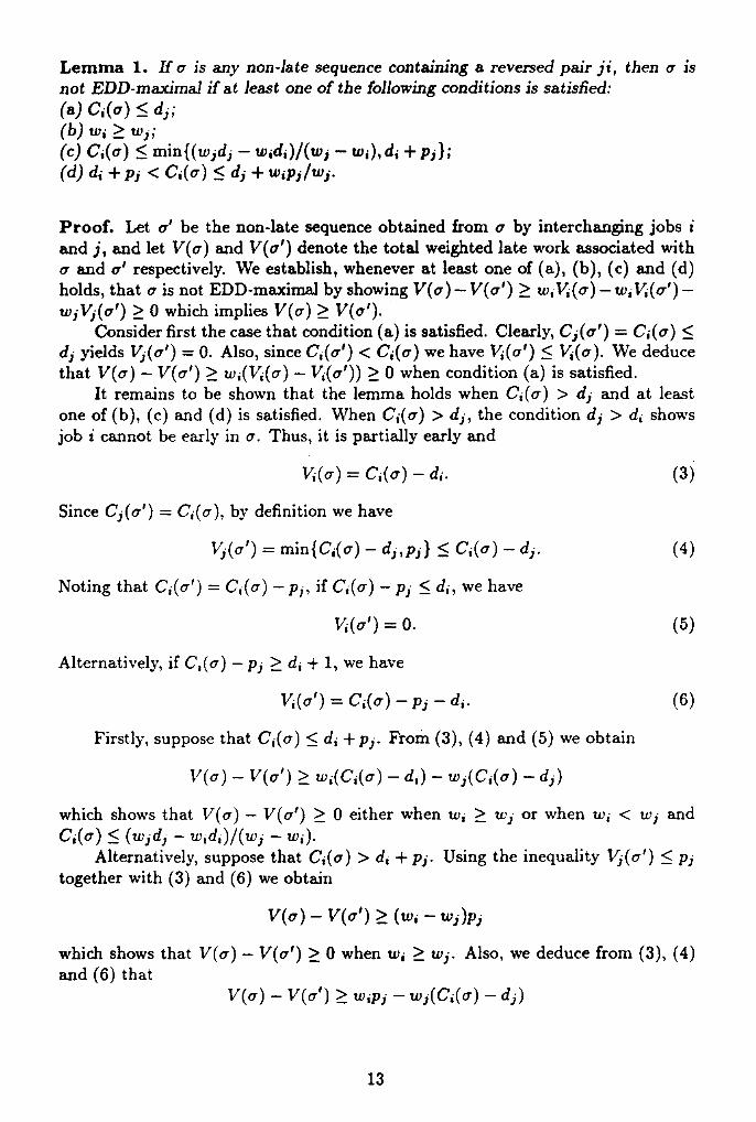
Lemma 1. If a is any non-late sequence containing a reversed pair ji, then a isnot EDD-maximal if at least one of the following conditions is satisfied:(a) Ci (a) 5 di;(b) wi > wi;(c) Ci(a) 5 min { (widi – widi )/(wi – wi ), di + pi} ;(d) di + pi < Ci (a) 5 di +wipi/wi.

Proof. Let a' be the non-late sequence obtained from a by interchanging jobs iand j, and let V(a) and V(a') denote the total weighted late work associated witha and a' respectively. We establish, whenever at least one of (a), (b), (c) and (d)holds, that a is not EDD-maximal by showing V(a)–V(a') w,V,(a)–w,V,(a')–wiVi (a s ) > 0 which implies V(a) > V(a').

Consider first the case that condition (a) is satisfied. Clearly, Ci(a') = Ci (a) <di yields Vi (cr') = 0. Also, since C,(a') < C,(a) we have V,(a') V,(a). We deducethat V(a) – V(a') > w,(V,(a)– Vs(a s ))> 0 when condition (a) is satisfied.

It remains to be shown that the lemma holds when Cs (a) > di and at leastone of (b), (c) and (d) is satisfied. When C,(a) > di , the condition di > d, showsjob i cannot be early in a. Thus, it is partially early and

Vi (a)= Ci (a) – di . (3)

Since Ci (a') = C,(a), by definition we have

Vi (a 1 ) = min{Ci(a) – cli ,pi } Ci(a)– di . (4)

Noting that Ci (a') = C (a) – p,, if C,(a) – pi 5 di , we have

Vi (a s ) = O. (5)

Alternatively, if C,(a) – p i > di + 1, we have

Vi (a 1 ) = Ci(a) – pi – d,. (6)

Firstly, suppose that Ci(a) < di + pi . From (3), (4) and (5) we obtain

V(a) – V(a l ) wi(C,(a) – d,) – wi (Ci(a) – di)

which shows that V(a) – V(a') > 0 either when w i > w; or when w i < wi andCi(a) (widi – w,d,)/(wi – wi)•

Alternatively, suppose that Ci (a) > di + pi . Using the inequality Vi (a') 5 p;together with (3) and (6) we obtain

V(a) – V(a s) (wi – wi)pi

which shows that V(a) – V(a') > 0 when w i > wi . Also, we deduce from (3), (4)and (6) that

V(a) – V(a') w ipi – wi(Ci(a ) – di)

13

which shows that V(a) – V(a') > 0 when Ci(a) < di + wspi /wi . Therefore,V(a)–V(a')> 0 either when w, > wi or when w, < wi and C,(a) < di +w,pi/wi.

It is now clear from the analysis of the cases C,(a) < pi and Ci(a) > d,+pithat if (b) holds, then V(a) > V(cr'). When w, < wi so that (b) is not satisfied,it is apparent from the analysis of the case Ci(a) < di + pi that if (c) holds, thenV(a) > V(cr i), and from the analysis of the case Ci(a) > + pi that if (d) holds,then V(a) V(a'). q

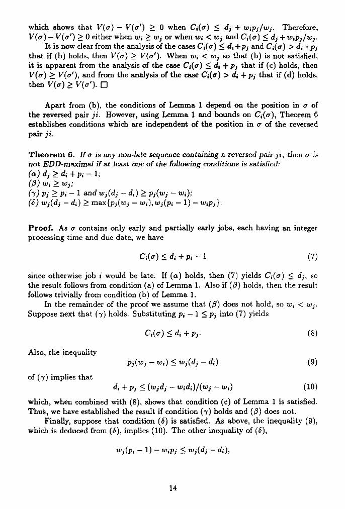
Apart from (b), the conditions of Lemma 1 depend on the position in a ofthe reversed pair However, using Lemma 1 and bounds on C,(a), Theorem 6establishes conditions which are independent of the position in a of the reversedpair ji.

Theorem 6. If a is any non-late sequence containing a reversed pair ji, then a isnot EDD-maximal if at least one of the following conditions is satisfied:(a) di > + pi – 1;(13) iv; wi;(7) pi- 1 and wi (di – cli )> pi (wi – wi);(5) wi (di – di) max{Ri (w; – wi ),wi (pi – 1) – wipi)•

Proof. As a contains only early and partially early jobs, each having an integerprocessing time and due date, we have

Ci(a) < di + pi - 1

(7)

since otherwise job i would be late. If (a) holds, then (7) yields C,(a) < di , sothe result follows from condition (a) of Lemma 1. Also if (0) holds, then the resultfollows trivially from condition (b) of Lemma 1.

In the remainder of the proof we assume that (fl) does not hold, so w, < wi.Suppose next that (-y) holds. Substituting p, - 1 < p i into (7) yields

Ci(cr) di + pi. (8)

Also, the inequalitypi (wi – w i ) wi(di - di)

(9)

of (7 ) implies thatd, + pi < – w,d,)/(wi – w,) (10)

which, when combined with (8), shows that condition (c) of Lemma 1 is satisfied.Thus, we have established the result if condition (7) holds and (0) does not.

Finally, suppose that condition (5) is satisfied. As above, the inequality (9).which is deduced from (b), implies (10). The other inequality of (5),

wi (pi – 1) – wipi 5_ wi (di – di),

14

which, when combined with (7), shows that

C,(cr) < + p, - 1 < di + wipi /wi . (11)

Now if Ci(a) < d, + pi , then (10) shows that condition (c) of Lemma 1 holds.Alternatively, if C,(cr) > + pi , then (11) shows that condition (d) of Lemma 1 issatisfied. Thus, in both cases at least one condition of Lemma 1 holds to give therequired result. 0

Next, we establish a lower bound on the completion time of job i of a reversedpair ji in an EDD-maximal sequence.

Theorem 7. If a is an EDD-maximal non-late sequence containing a reversed pairji, then

C,(a) _� min{1 + L(wj di – w,di )/(wi – wi th 1 + 141 + w ipi /wijI. (12)

Furthermore, if pi > p, – 1, then

Ci(a) 1 + I(tvi – widi )/(wi – (13)

Proof. Since a is an EDD-maximal sequence, none of the conditions of Lemma 1are satisfied. If C,(a) < d, + pi , then because (c) does not hold, we have

C1( a ) > (widi – widi )/(wi – wi)• (14)

Similarly, if Ci (a) > di + pi , the violation of (d) yields

Ci (o) > di +

(15)

Since C,(a) < d, + pi or C,(a) > d, + pi , either (14) or (15) holds. Using theintegrality of C,(a) and the lower bound given by the smaller of the right handsides of (14) and (15), we deduce inequality (12).

We now establish inequality (13) when pi > p, – 1. Combining C,(a) < d, +pi –1, which holds because job i is non-late, with p, –1 < pi yields C, (a) < di + pi.Thus, (14) holds in this case, from which we use the integrality of C,(cr) to obtain(13). 0

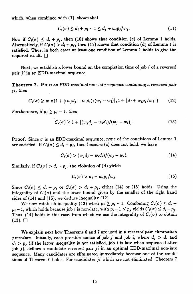
We explain next how Theorems 6 and 7 are used in a reversed pair eliminationprocedure. Initially, each possible choice of job j and job i, where di > di anddi > pi (if the latter inequality is not satisfied, job i is late when sequenced afterjob j), defines a candidate reversed pair ji in an optimal EDD-maximal non-latesequence. Many candidates are eliminated immediately because one of the condi-tions of Theorem 6 holds. For candidates ji which are not eliminated, Theorem 7

15

defines a lower bound of the form C, > czji on the completion time of job i if ji is a.reversed pair of an EDD-maximal non-late sequence. Let LB,. be a lower bound onthe total weighted late work for the constrained problem in which ji is forced to bea reversed pair, i.e., job i is constrained to be sequenced immediately after job j andhave a completion time which satisfies a ii < < +pi -1. If ji forms a reversedpair in an optimal sequence, then LB,; < UB, where UB is obtained by applyingour dynamic programming heuristic of Section 4 (although any other upper boundon the total weighted late work can be used). Thus, if LB .ii > UB, the reversedpair ji cannot exist in an optimal non-late sequence and, hence, is eliminated as acandidate.

It remains to define the lower bound LBii on the total weighted late work forthe constrained problem which is used in the reversed pair elimination procedure.We adopt a similar approach to that for obtaining lower bounds for use in thelateness test. Since job j is constrained to be early and job i is constrained to becompleted not after time di + p, – 1 (and not before time a, i ), we enforce theseconstraints by assigning large weights to jobs j and i and resetting the due date ofjob i to di + p, – 1. Thus, to obtain LB,„ we solve the preemptive total weightedlate work problem having processing times A, = ph (h = 1, ... ,n), weights wh' = wh(h = 1, ,n; h i; h j) and w: = w; = co and due dates dri, = dh (h = 1, , n;h i) and di, = d,+p,-1. If LB ?) , is the total weighted late work for this preemptiveproblem, obtained by applying the Preemptive Scheduling Algorithm of Section 1,our lower bound is defined by LB .? , = LW), + – di ): since the late work forjob i is zero in the preemptive problem, but is at least a) , – di in the constrainedproblem, the final term in LB;, accounts for this difference. We now give a formaljustification the use of LB) , as a lower bound on the total weighted late work forthe. (non-preemptive) constrained problem.

Theorem 8. No optimal EDD-maximal solution contains a reversed pair which iseliminated by the reversed pair elimination procedure.

Proof. It is sufficient to establish that LB) , is a lower bound on the total weightedlate work for the constrained problem. Let a denote an optimal non-late sequencefor the constrained problem which defines Vh (a) as the late work for job h (h =1, , n), where Vh (a) = ph if h does not appear in a. The constraint aj , < <di + p, – 1 and the observation that aj , > d, implies job i is partially early in a.Since job j is early in a, we obtain

w,V,(a)+ wj y,(a) = w,V,(a) = w,(C,(cr)– d i ) w,(aj , – d,). (16)

Suppose that a is evaluated with respect to the data for the preemptive problem togive .VI:(a) as the late work for job h (h = 1, ,n). We have VAcr) = VI(a) = 0since jobs i and j are early with respect to the due dates and d'j , whereas Vi:(a) =Vh (a) for h = n, h i and h j. Therefore, we deduce from (16) that

E whVh(a) � E whil(a)+ w,(aj , - di ) + tv.(a cit) = LB I,h=1 h=1

16

where the final inequality holds because LBO, is the minimum total weighted latework for the preemptive problem. It is now apparent that 1,13 i, is a valid lowerbound for use in our reversed pair elimination procedure. q

In view of the above analysis, we modify each set Ait so that it contains onlythose jobs i such that ji remains a candidate after the reversed pair eliminationprocedure is applied and such that aji < t < d1 +p, —1. The modified fij , is used inthe computation of our lower bounds and increases their effectiveness. Also, thesemodified sets can be used in the dynamic programming algorithm of Section 3.

7. The branch and bound algorithmIn this section, we give full details of our branch and bound algorithm. Prior

to applying branch and bound, the earliness test of Section 5.1 is first applied.Then, we use the dynamic programming heuristic of Section 4 (incorporating theredundant state elimination procedure of Section 5.3) to generate an upper bound.To economize on storage space, the recursion is used to obtain the value UB only,with no attempt made to find a corresponding sequence of jobs. (The branchand bound algorithm finds a sequence with total weighted late work of UB or less.)Having obtained UB, the lateness test of Section 5.2 is applied to reduce further thenumber of jobs. The final preprocessing step applies the reversed pair eliminationprocedure of Section 6.

The branch and bound algorithm first computes the lower bound of Section 4(using redundant state elimination and the modified sets Aft ), and the correspond-ing non-late 'sequence' of jobs is obtained. If there are no repeated jobs in thisnon-late 'sequence', then it provides an optimal solution at the root node of thesearch tree. Otherwise, a repeated job i is found in the non-late 'sequence'. Abinary branching rule constrains job i so that either it is sequenced in EDD orderor it is not in EDD order. When job i is sequenced in EDD order, i is removedfrom each set Ajt and the recursion equations for Mt) are modified from thosegiven in Section 4 by deleting the expression f:_ 1 (t) + w,p, which corresponds tocases that job i is late or is deferred. Alternatively, when job i is not sequencedin EDD order (it is either late or deferred), the values of Mt) are computed usingf•(t) = f:_/(t)+wip,. In either case, job i cannot again appear twice in a 'sequence'obtained from the lower bounding procedure.

For any node of the search tree in which the lower bound is not greater thanthe current upper bound and the corresponding non-late 'sequence' is feasible, theupper bound is updated and the node is discarded. A node is also discarded if itslower bound exceeds the current upper bound. A newest active node search selectsa node from which to branch.

8. Computational experienceThe algorithm was tested on problems with numbers of jobs ranging from

17

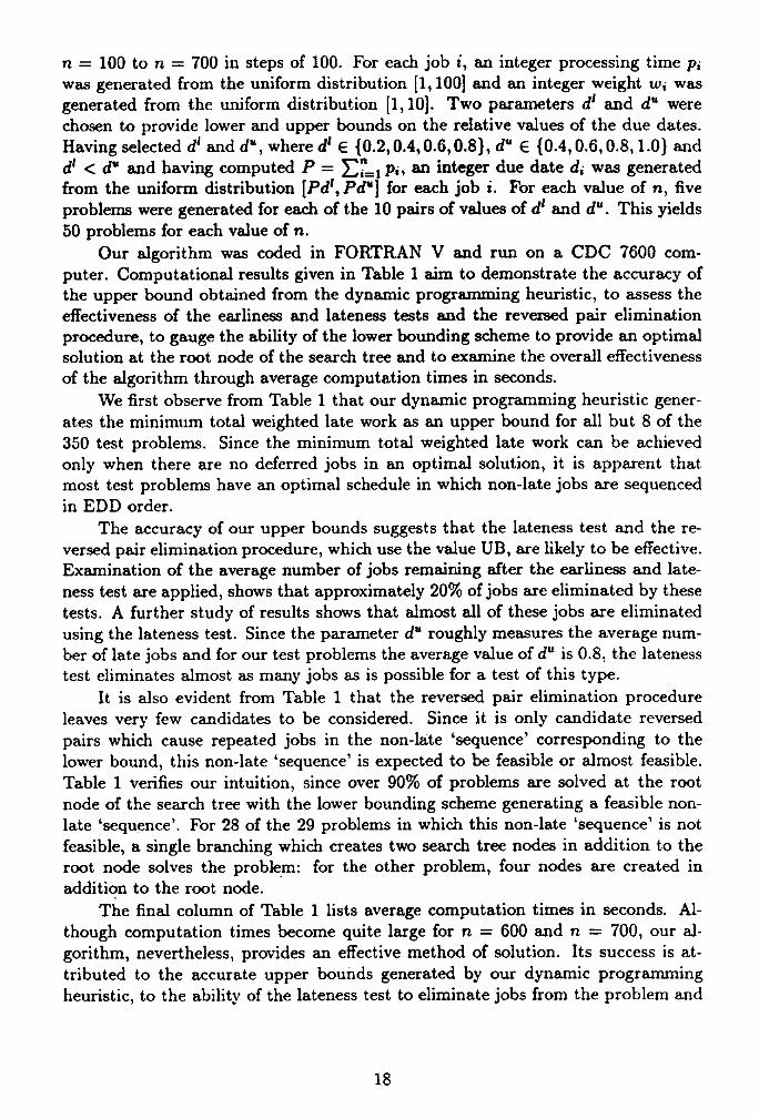
n = 100 to n = 700 in steps of 100. For each job i, an integer processing time p,was generated from the uniform distribution [1,100] and an integer weight w, wasgenerated from the uniform distribution [1,14 Two parameters d' and d" werechosen to provide lower and upper bounds on the relative values of the due dates.Having selected d' and d", where di E {0.2, 0.4, 0.6, 0.8}, d u E {0.4, 0.6, 0.8, 1.0} and

< du and having computed P = pi, an integer due date di was generatedfrom the uniform distribution [Pd', Pd"] for each job i. For each value of n, fiveproblems were generated for each of the 10 pairs of values of d' and d". This yields50 problems for each value of n.

Our algorithm was coded in FORTRAN V and run on a CDC 7600 com-puter. Computational results given in Table 1 aim to demonstrate the accuracy ofthe upper bound obtained from the dynamic programming heuristic, to assess theeffectiveness of the earliness and lateness tests and the reversed pair eliminationprocedure, to gauge the ability of the lower bounding scheme to provide an optimalsolution at the root node of the search tree and to examine the overall effectivenessof the algorithm through average computation times in seconds.

We first observe from Table 1 that our dynamic programming heuristic gener-ates the minimum total weighted late work as an upper bound for all but 8 of the350 test problems. Since the minimum total weighted late work can be achievedonly when there are no deferred jobs in an optimal solution, it is apparent thatmost test problems have an optimal schedule in which non-late jobs are sequencedin EDD order.

The accuracy of our upper bounds suggests that the lateness test and the re-versed pair elimination procedure, which use the value UB, are likely to be effective.Examination of the average number of jobs remaining after the earliness and late-ness test are applied, shows that approximately 20% of jobs are eliminated by thesetests. A further study of results shows that almost all of these jobs are eliminatedusing the lateness test. Since the parameter du roughly measures the average num-ber of late jobs and for our test problems the average value of d" is 0.8, the latenesstest eliminates almost as many jobs as is possible for a test of this type.

It is also evident from Table 1 that the reversed pair elimination procedureleaves very few candidates to be considered. Since it is only candidate reversedpairs which cause repeated jobs in the non-late 'sequence' corresponding to thelower bound, this non-late 'sequence' is expected to be feasible or almost feasible.Table 1 verifies our intuition, since over 90% of problems are solved at the rootnode of the search tree with the lower bounding scheme generating a feasible non-late 'sequence'. For 28 of the 29 problems in which this non-late 'sequence' is notfeasible, a single branching which creates two search tree nodes in addition to theroot node solves the problem: for the other problem, four nodes are created inaddition to the root node.

The final column of Table 1 lists average computation times in seconds. Al-though computation times become quite large for n = 600 and n = 700, our al-gorithm, nevertheless, provides an effective method of solution. Its success is at-tributed to the accurate upper bounds generated by our dynamic programmingheuristic, to the ability of the lateness test to eliminate jobs from the problem and

18

Table 1

Computational results

n NHO ANJR ANRP NSRN ACT

100 46 73 2.5 47 0.91

200 49 160 2.7 45 3.44

300 50 246 2.2 45 7.84

400 49 325 2.2 46 12.98

500 49 387 1.9 44 20.71

600 49 487 1.8 49 30.27

700 50 555 4.4 45 43.16

NHO: number of problems (out of 50) for which the dynamic programming

heuristic is optimal.

ANJR: average number of jobs remaining after the reduction tests are ap-

plied.

ANRP: average number of candidate reversed pairs remaining after the re-

versed pair elimination procedure is applied.

NSRN: number of problems (out of 50) solved at the root node of the search

tree.

ACT: average computation time in seconds.

19

to the lower bounding procedure which, through the aid of the reversed pair elimi-nation procedure, enables an optimal solution to be generated at the root node ofthe search tree in many cases.

9. Concluding remarksWe have established the computational complexity of preemptive and non-

preemptive scheduling on a single machine to minimize total weighted late work.The preemptive problem is solvable in 0(n log n) time using our algorithm of Sec-tion 1. Also, through the use of Theorem 3 which shows that early and partiallyearly jobs are sequenced almost in EDD order, we have derived a dynamic program-ming algorithm for the non-preemptive problem which requires pseudopolynomialtime. Since the non-preemptive total late work problem is already known to beNP-hard, there is little hope of finding a polynomial algorithm.

This paper also gives a practical branch and bound algorithm for the non-preemptive total weighted late work problem. The lateness test of Section 5 andthe reversed pair elimination procedure of Section 6 have a major influence on thesuccess of the algorithm. Armed with these devices to restrict the search, our lowerbounding scheme, derived using the dynamic programming state-space relaxationmethod, produces an optimal sequence in many cases. Even if it does not solve theproblem at the root node, the branch and bound search tree is likely to be smallsince all our test problems are solved after at most two branchings.

AcknowledgementThe research by the first author was supported by a grant from King Abdul-

Aziz University, Jeddah, Saudi Arabia. The authors are grateful to an anonymousreferee for suggestions on improving the structure of the paper.

References[1] T.S. Abdul-Razaq and C.N. Potts, 1988. Dynamic Programming State-Space

Relaxation for Single Machine Scheduling. Journal of the Operational Re-search Society 39, 141-152.

[2] J. Blazewicz, 1984. Scheduling Preemptible Tasks on Parallel Processors withInformation Loss, Technique et Science Informatique 3, 415-420.

[3] M. Blum, R.W. Floyd, V. Pratt, R.L. Rivest and R.E. Tarjan, 1973. TimeBounds for Selection, Journal of Computer and System Sciences 7, 448-461.

[4] N. Christofides, A. Mingozzi and P. Toth, 1981. State-Space Relaxation Pro-cedures for the Computation of Bounds to Routing Problems, Networks 11,145-164.

[5] R.M. Karp, 1972. Reducibility among Combinatorial Problems, in Complexityof Computer Computations, J.W. Thatcher and J.W. Miller (eds.), PlenumPress, New York, pp. 85-103.

20

[6] E.L. Lawler, 1976. Combinatorial Optimization: Networks and Matroids, Holt,Rinehart and Winston, New York.

[7] E.L. Lawler, 1977. A Pseudopolynomiar Algorithm for Sequencing Jobs toMinimize Total Tardiness, Annals of Discrete Mathematics 1, 331-342.

[8] E.L. Lawler, and J.M. Moore, 1969. A Functional Equation and its Applicationto Resource Allocation and Sequencing Problems, Management Science 16,77-84.

[9] J.K. Lenstra, A.H.G. Rinnooy Kan and P. Brucker, 1977. Complexity of Ma-chine Scheduling Problems, Annals of Discrete Mathematics 1, 343-362.

[10] C.N. Potts and L.N. Van Wassenhove, 1985. A Branch and Bound Algorithmfor the Total Weighted Tardiness Problem, Operations Research 33, 363-377.

[11] C.N. Potts and L.N. Van Wassenhove, 1988. Algorithms for Scheduling a Sin-gle Machine to Minimize the Weighted Number of Late Jobs, ManagementScience 34, 843-858.

[12] C.N. Potts and L.N. Van Wassenhove, 1992. Single Machine Scheduling toMinimize Total Late Work, Operations Research 40, to appear.

[13] A. Schonhage, M. Paterson and M. Pippenger, 1976. Finding the Median,Journal of Computer and System Sciences 13, 189-199.

21