Embed Size (px)
Citation preview

Università degli Studi di Trento
Facoltà di Scienze Matematiche Fisiche e NaturaliDipartimento di Matematica
Dottorato in MatematicaCiclo XXI
On algebraic and statistical properties ofAES-like ciphers
Anna Rimoldi
Supervisor: Prof. M. Sala
Head of PhD School: Prof. A. Valli


Università degli Studi di Trento
Facoltà di Scienze Matematiche Fisiche e Naturali
Dipartimento di Matematica
Dottorato in MatematicaCiclo XXI
On algebraic and statistical properties ofAES-like ciphers
Ph.D.Thesis of:Anna Rimoldi
Supervisors:Prof. M. Sala
Head of PhD School:Prof. A. Valli


Contents
I Preliminaries 1
1 Preliminaries and notation 31.1 Algebraic background . . . . . . . . . . . . . . . . . . . . . . . . . . . 3
1.1.1 Finite Fields . . . . . . . . . . . . . . . . . . . . . . . . . . . . 41.1.2 Permutation polynomials . . . . . . . . . . . . . . . . . . . . . 4
1.2 Block ciphers . . . . . . . . . . . . . . . . . . . . . . . . . . . . . . . 51.2.1 Perfect secrecy . . . . . . . . . . . . . . . . . . . . . . . . . . 101.2.2 What do we mean by a “good” Block Cipher? . . . . . . . . . 111.2.3 Cryptanalytic scenarios . . . . . . . . . . . . . . . . . . . . . . 13
1.3 Cryptographic hash functions . . . . . . . . . . . . . . . . . . . . . . 161.4 Statistical tests . . . . . . . . . . . . . . . . . . . . . . . . . . . . . . 18
2 A description of AES, SERPENT and PRESENT 232.1 The AES cryptosystem . . . . . . . . . . . . . . . . . . . . . . . . . . 25
2.1.1 SubBytes . . . . . . . . . . . . . . . . . . . . . . . . . . . . . 262.1.2 Mixing Layer . . . . . . . . . . . . . . . . . . . . . . . . . . . 272.1.3 Key schedule . . . . . . . . . . . . . . . . . . . . . . . . . . . 282.1.4 Small scale variants of the AES . . . . . . . . . . . . . . . . . 29
2.2 The SERPENT cryptosystem . . . . . . . . . . . . . . . . . . . . . . 302.2.1 A SERPENT round . . . . . . . . . . . . . . . . . . . . . . . 302.2.2 The Linear transformation . . . . . . . . . . . . . . . . . . . . 312.2.3 The SERPENT’s key schedule . . . . . . . . . . . . . . . . . . 32
2.3 PRESENT: an ultra-lightweight block cipher . . . . . . . . . . . . . . 332.3.1 sBoxLayer . . . . . . . . . . . . . . . . . . . . . . . . . . . . . 332.3.2 pLayer . . . . . . . . . . . . . . . . . . . . . . . . . . . . . . . 33
3 On the AES cryptanalysis 353.1 Statistical attacks . . . . . . . . . . . . . . . . . . . . . . . . . . . . . 35
3.1.1 Distinguishing Attacks . . . . . . . . . . . . . . . . . . . . . . 363.2 Structural attacks . . . . . . . . . . . . . . . . . . . . . . . . . . . . . 37
3.2.1 Square attack . . . . . . . . . . . . . . . . . . . . . . . . . . . 38
i

3.2.2 Partial Sum . . . . . . . . . . . . . . . . . . . . . . . . . . . . 403.2.3 Impossible Differentials . . . . . . . . . . . . . . . . . . . . . . 423.2.4 Collision Attacks . . . . . . . . . . . . . . . . . . . . . . . . . 423.2.5 Boomerang attack . . . . . . . . . . . . . . . . . . . . . . . . 42
3.3 First algebraic attacks . . . . . . . . . . . . . . . . . . . . . . . . . . 463.3.1 Continued fractions . . . . . . . . . . . . . . . . . . . . . . . . 473.3.2 Polynomial system approach . . . . . . . . . . . . . . . . . . . 48
3.4 Alternative representations . . . . . . . . . . . . . . . . . . . . . . . . 503.4.1 BES . . . . . . . . . . . . . . . . . . . . . . . . . . . . . . . . 503.4.2 Polynomial system . . . . . . . . . . . . . . . . . . . . . . . . 543.4.3 Toli-Zanoni’s remark . . . . . . . . . . . . . . . . . . . . . . . 56
3.5 Dual ciphers . . . . . . . . . . . . . . . . . . . . . . . . . . . . . . . . 573.5.1 Square dual ciphers . . . . . . . . . . . . . . . . . . . . . . . . 583.5.2 Dual ciphers modifying the irreducible polynomial . . . . . . . 603.5.3 Logarithmic dual ciphers . . . . . . . . . . . . . . . . . . . . . 603.5.4 Self-dual ciphers . . . . . . . . . . . . . . . . . . . . . . . . . 61
3.6 S-boxes equivalence . . . . . . . . . . . . . . . . . . . . . . . . . . . . 623.6.1 Linear equivalence . . . . . . . . . . . . . . . . . . . . . . . . 643.6.2 Affine equivalence . . . . . . . . . . . . . . . . . . . . . . . . . 643.6.3 Extension . . . . . . . . . . . . . . . . . . . . . . . . . . . . . 653.6.4 Equivalences in the AES cryptosystem . . . . . . . . . . . . . 66
II Our Results 67
4 A new representation 694.1 Some preliminary results . . . . . . . . . . . . . . . . . . . . . . . . . 704.2 A first representation . . . . . . . . . . . . . . . . . . . . . . . . . . . 73
4.2.1 Application to AES . . . . . . . . . . . . . . . . . . . . . . . . 774.2.2 Application to PRESENT . . . . . . . . . . . . . . . . . . . . 794.2.3 Application to SERPENT . . . . . . . . . . . . . . . . . . . . 80
4.3 An “orbit” representation . . . . . . . . . . . . . . . . . . . . . . . . . 814.3.1 Application to AES . . . . . . . . . . . . . . . . . . . . . . . . 854.3.2 Application to PRESENT . . . . . . . . . . . . . . . . . . . . 864.3.3 Application to SERPENT . . . . . . . . . . . . . . . . . . . . 86
4.4 Other representations of this kind . . . . . . . . . . . . . . . . . . . . 874.5 Further remarks . . . . . . . . . . . . . . . . . . . . . . . . . . . . . . 87
4.5.1 First approach . . . . . . . . . . . . . . . . . . . . . . . . . . 894.5.2 Using the order of the elements . . . . . . . . . . . . . . . . . 90
ii

4.6 Some results on a weaker notion of linearity . . . . . . . . . . . . . . 92
5 A related-key attack 975.1 Related-key distinguishing attacks . . . . . . . . . . . . . . . . . . . . 975.2 Our setting . . . . . . . . . . . . . . . . . . . . . . . . . . . . . . . . 975.3 The AES case . . . . . . . . . . . . . . . . . . . . . . . . . . . . . . . 995.4 Numerical results . . . . . . . . . . . . . . . . . . . . . . . . . . . . . 1005.5 Comments . . . . . . . . . . . . . . . . . . . . . . . . . . . . . . . . . 105
6 Appendix 109
Bibliography 116
iii


Acknowledgment
First of all, I would like to express sincere gratitude to my supervisor Prof. Mas-similiano Sala for his encouragement, his advice and research support throughout myMaster’s and PhD studies.
I am grateful to my thesis defense Committee, Prof. Carlo Traverso, Prof. TeoMora and Dr. Ludovic Perret, for their helpful suggestions.
I would like to thank the whole Department of Mathematics of University ofTrento for its support, especially Prof. Andrea Caranti, Prof. Marco Sabatini andProf. Alberto Valli.
Furthermore, thanks to Dr. Giacomo Aletti, Dr. Guido Bertoni, Prof. FrancescaDalla Volta, Dr. Lilli Fragneto, Dr. Ilia Toli for their helpful comments.
Sincere thanks to Dr. Fabrizio Caruso for helping me in the more computationalpart of this work and for many interesting discussions.
I want to thank all my fellow PhD students and in particular Federica, Elisa,Stefano e Philipp; I want also thank Lara Maines for her scientific contributions andall the fantastic guys in our group.
My last but important acknowledgment is for my family and for my friends Clau-dia, Marco, Paolo and Roberto and Yudis.
v


Some Notation
N = 0, 1, 2, . . .Fq finite field with q elementsV = (Fq)r vector space over Fq of dimension rSym(V ) symmetric group on VAlt(V ) alternating group on VGL(V ) group of all linear permutations of VC⊥ the orthogonal space of any vector space C < V w.r.t. the standard
scalar product in VIm(f) image of any function f : S → T , with S, T any sets.w(v) Hamming weight of the vector v ∈ (Fq)r
m Rijndael polynomial, m = x8 + x4 + x3 + x+ 1 ∈ F2[x]
d`e is minn ∈ Z|n ≥ ` (ceiling)o(σ) the order of permutation σi.e. id este.g. exempli gratiaw.l.o.g. without loss of generalityw.r.t. with respect tos.t. such thatNIST National Institute for Standards and Technology (US)
vii

Introduction
The Advanced Encryption Standard (AES) is nowadays the most widespread blockcipher in commercial applications. It represents the state-of-art in block cipher de-sign and provides an unparalleled level of assurance against all known cryptanalytictechniques, except for its reduced versions. Moreover, there is no known efficient wayto distinguish it from a set of random permutations.
The AES (and other modern block ciphers) presents a highly algebraic structure,which led researchers to exploit it for novel algebraic attacks. These tries have beenunsuccessful, except for academic reduced versions.
Starting from an intuition by I. Toli, we have developed a mixed algebraic-statisticalattack. Using the internal algebraic structure of any AES-like cipher, we build an alge-braic setting where a related-key (statistical) distinguishing attack can be mounted.Our data reveals a significant deviation of the full AES-128 from a set of randompermutations. Although there are recent successful related-key attacks on the fullAES-192 and the full AES-256 (with non-practical complexity), our attack would bethe first-ever practical distinguishing attack on the full AES-128 (to the best of ourknowledge).
In Part I we provide some preliminaries and sketch a survey of known attacks onthe AES versions, in particular on AES-128.
In Chapter 1 we give some basic algebraic background and we summarize thenotion of a block cipher, with its link to hash functions. In particular, we introduce theclass of translation based cryptosystems, which are ciphers enjoying some interestingalgebraic properties.
In Chapter 2 we describe the three main translation-based cryptosystems: AES,SERPENT and PRESENT.
In Chapter 3 we briefly report on known attacks on AES, including structural,statistical and algebraic attacks. This chapter can be skipped in a first reading ofthis thesis.
ix

In Part II we present our attack and its algebraic setting.In Chapter 4 we give some algebraic embeddings of a translation based cipher into
a much larger cipher. These embeddings are designed to lower the non-linearity ofthe encryption functions. Two of them are practical and can be applied in principleto AES, PRESENT and SERPENT. In particular, the orbit representation works wellwith AES-128 and PRESENT. However, with group theory proofs we also show thatno representation/embedding can completely linearize the full AES-128.
In Chapter 5 we use the orbit representation for AES-128 and we are able tofind sets of related matrices with related keys such that the encryption action can beshown to differ significantly from the behavior of a set of random permutations. Ourattack may be seen as an extremely refined version of a Marsaglia Diehard test.
x

Part I
Preliminaries
1


Preliminaries and notation
In this chapter we recall well-known results in group theory and finite field theory[LN97] in order to fix the notation we will use in the sequel.We also outline some basic ideas about block ciphers, their security level and theircryptanalysis. Definitions and results are mainly from [Sti95], [CW09] and [DR02].In the last section we will give an overview of the statistical tests adopted by NIST[NIS00] to evaluate the random behavior of the AES candidates.
1.1 Algebraic background
Let n ≥ 2 be an integer. Let V = (F2)n be the vector space over the finite field F2
of dimension n. We denote by Sym(V ) and Alt(V ), respectively, the symmetric andalternating group on V . We denote by GL(V ) the group of all linear permutations ofV . We recall the well-known formulas:
|Sym(V )| = 2n!, |Alt(V )| = 2n!
2|GL(V )| =
n−1∏h=0
(2n − 2h) < 2n2
.
Given a finite groupG, we say thatG can be linearized if there is an injective morphismρ : G→ GL(V ) (this is called a “faithful representation” in representation theory).
Definition 1.1.1. A (linear) representation of a group G over a vector space V is agroup homomorphism ρ : G→ GL(V ). If ρ is injective, it is called faithful.
If G can be linearized, then, for any element g ∈ G, we can compute a matrixMg corresponding to the action of g over V (via ρ). The matrix computation is easy,since it is enough to evaluate g on a basis of V .If ρ : G → GL(V ) is a representation of G on V , then we often write gv insteadof ρ(g)v, if no confusion arises. Also, G is said to act linearly on V , and V iscalled a G-module. The degree of the representation is by definition the dimensionof V . By taking V = 2|G| we can always linearize G over V via the so-called regularrepresentation, but of course this is huge and usually impractical.
Definition 1.1.2. Let G = g1, . . . , gn be a finite group. Let V be a vector spacewith basis eg1 , . . . , egn. The regular representation ρ : G → GL(V ) is defined byρ(gi)(egj) = egigj (where gigj is the group product).
3

Chapter 1. Preliminaries and notation
Definition 1.1.3 (Equivalence of Representations). Two representations ρ1 and ρ2
over a vector space V are said to be equivalent if they are related by conjugation, i.e.there is h ∈ GL(V ) such that ρ2(g) = h(ρ1(g))h−1, ∀g ∈ G.
1.1.1 Finite Fields
For any prime p and any positive m ∈ N, Fpm is the field with pm elements(unique up to field isomorphism). It contains an isomorphic copy of Fp and can thusbe thought as an extension of Fp. On the other hand, we can construct any Fqs fromFq with q = pm elements, as follows.Let f ∈ Fq[x] be an irreducible polynomial of degree m. We can consider the quotientR = Fq[x]/(f), where (f) is the ideal generated by f in Fq[x]. By considering thenatural projection π : Fq[x]→ R, we call α = π(x) and clearly any element of R canbe uniquely expressed as a polynomial in α of degree less than m:
R =
m−1∑i=0
aiαi | ai ∈ Fq
with the condition f(α) = 0.
Theorem 1.1.4. R = Fq[x]/(f) is a field and R ∼= Fqm.
We denote by F∗q the multiplicative group of non-zero elements of Fq.
Theorem 1.1.5. For any finite field Fq, the multiplicative group F∗q is cyclic.
A generator of the cyclic group F∗q is called a primitive element of Fq.
Definition 1.1.6. An irreducible polynomial f ∈ Fq[x] is primitive if its roots areprimitive elements.
We conclude this subsection by observing that for any q and m there are indeedirreducible polynomials of degree m over Fq and some of them are primitive.
1.1.2 Permutation polynomials
Definition 1.1.7. A polynomial f ∈ Fq[x] is a permutation polynomial of Fq if theassociated polynomial function f : c 7→ f(c) from Fq into Fq is a permutation of Fq.
If f is an affine map f : x 7→ ax+ b (a 6= 0), we say that f is a linear polynomial.
4
1.2. Block ciphers
We note the following easy results:
1. Every linear polynomial over Fq is a permutation polynomial of Fq.
2. The monomial xn is a permutation polynomial of Fq if and only if
gcd(n, q − 1) = 1.
Permutation polynomials of Fq of degree less then q can be combined by the operationof composition and subsequent reduction modulo xq − x. The set of permutationpolynomials of Fq of degree less then q forms a group, which is isomorphic to Sym(Fq).Then, the symmetric group Sym(Fq) and its subgroups can be represented as groupsof permutation polynomials.
Theorem 1.1.8. For q > 2, the symmetric group Sym(Fq) is generated by xq−2 andall linear polynomials over Fq.
1.2 Block ciphers
Block ciphers form an important class of cryptosystems in symmetric key cryp-tography. Stream ciphers [Rue92] form another class. We are interested only incryptosystems of type block ciphers. These are algorithms that encrypt and decryptblocks of data (with fixed length1) according to a shared secret key. They are com-monly used to provide confidentiality during information transmission and storage.We can formally describe such a cryptosystem using the following definition:
Definition 1.2.1. A cryptosystem is a pair (M,K), where:
• M is a finite set of possible messages (plaintexts, ciphertexts);
• K, the key-space, is a finite set of possible keys;
• we have encryption and decryption functions for any key k ∈ K:
φk :M→M, ψk :M→M, φk, ψk ∈ Sym(M)
such thatψk = (φk)
−1.
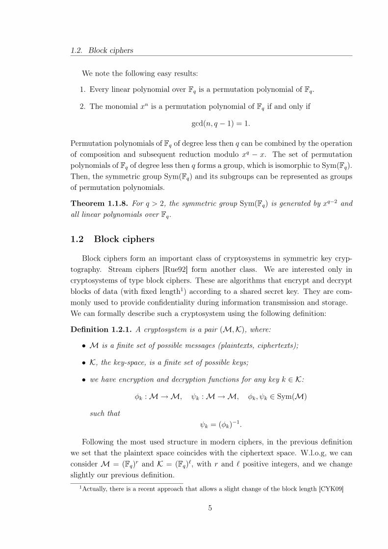
Following the most used structure in modern ciphers, in the previous definitionwe set that the plaintext space coincides with the ciphertext space. W.l.o.g, we canconsider M = (Fq)r and K = (Fq)`, with r and ` positive integers, and we changeslightly our previous definition.
1Actually, there is a recent approach that allows a slight change of the block length [CYK09]
5
Chapter 1. Preliminaries and notation
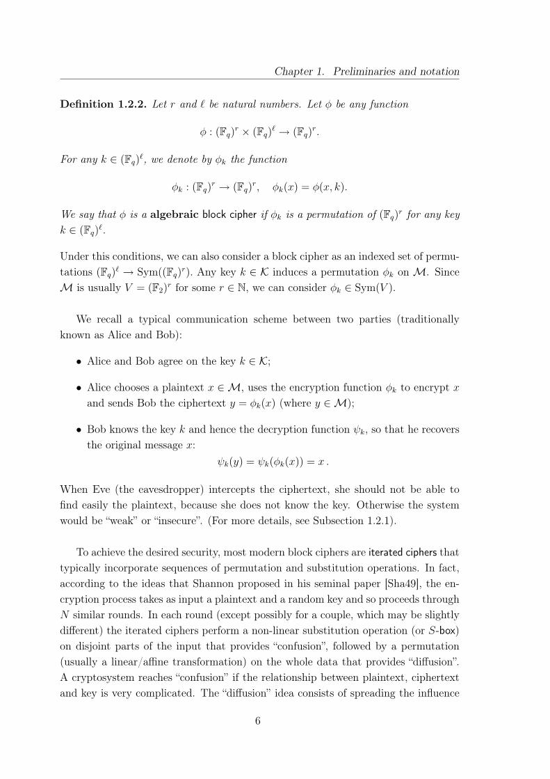
Definition 1.2.2. Let r and ` be natural numbers. Let φ be any function
φ : (Fq)r × (Fq)` → (Fq)r.
For any k ∈ (Fq)`, we denote by φk the function
φk : (Fq)r → (Fq)r, φk(x) = φ(x, k).
We say that φ is a algebraic block cipher if φk is a permutation of (Fq)r for any keyk ∈ (Fq)`.
Under this conditions, we can also consider a block cipher as an indexed set of permu-tations (Fq)` → Sym((Fq)r). Any key k ∈ K induces a permutation φk onM. SinceM is usually V = (F2)r for some r ∈ N, we can consider φk ∈ Sym(V ).
We recall a typical communication scheme between two parties (traditionallyknown as Alice and Bob):
• Alice and Bob agree on the key k ∈ K;
• Alice chooses a plaintext x ∈ M, uses the encryption function φk to encrypt xand sends Bob the ciphertext y = φk(x) (where y ∈M);
• Bob knows the key k and hence the decryption function ψk, so that he recoversthe original message x:
ψk(y) = ψk(φk(x)) = x .
When Eve (the eavesdropper) intercepts the ciphertext, she should not be able tofind easily the plaintext, because she does not know the key. Otherwise the systemwould be “weak” or “insecure”. (For more details, see Subsection 1.2.1).
To achieve the desired security, most modern block ciphers are iterated ciphers thattypically incorporate sequences of permutation and substitution operations. In fact,according to the ideas that Shannon proposed in his seminal paper [Sha49], the en-cryption process takes as input a plaintext and a random key and so proceeds throughN similar rounds. In each round (except possibly for a couple, which may be slightlydifferent) the iterated ciphers perform a non-linear substitution operation (or S-box)on disjoint parts of the input that provides “confusion”, followed by a permutation(usually a linear/affine transformation) on the whole data that provides “diffusion”.A cryptosystem reaches “confusion” if the relationship between plaintext, ciphertextand key is very complicated. The “diffusion” idea consists of spreading the influence
6
1.2. Block ciphers
of all parts of the input (plaintext and key) to all parts of the ciphertext. The op-erations performed in a round form the round function. The round function at theρ-th round (1 ≤ ρ ≤ N) takes as inputs both the output of the (ρ− 1)-th round andthe subkey k(ρ) (also called round-key). Any round key k(ρ) is constructed startingfrom a master key2 k of some specified length, e.g. k ∈ K = (F2)` (nowadays we have264 ≤ |K| ≤ 2256). The key schedule is a public algorithm (strictly dependent on thecipher) which constructs N + 1 subkeys (k(0), . . . , k(N)).
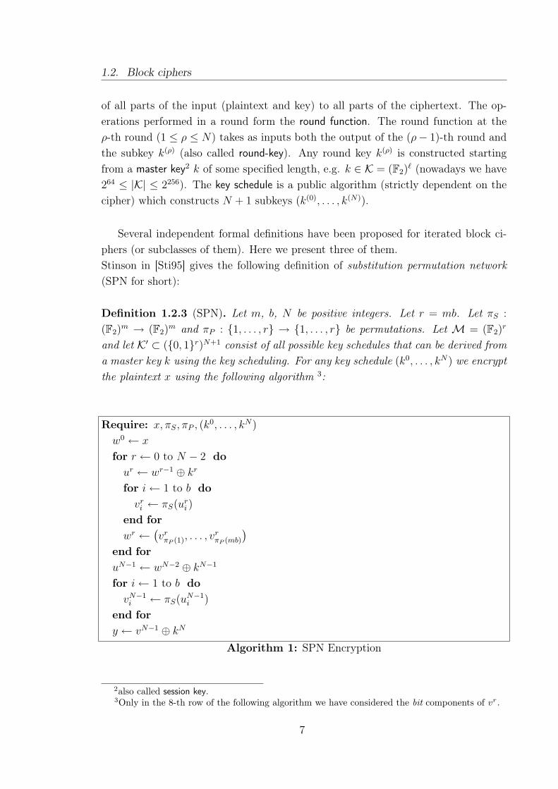
Several independent formal definitions have been proposed for iterated block ci-phers (or subclasses of them). Here we present three of them.Stinson in [Sti95] gives the following definition of substitution permutation network(SPN for short):
Definition 1.2.3 (SPN). Let m, b, N be positive integers. Let r = mb. Let πS :
(F2)m → (F2)m and πP : 1, . . . , r → 1, . . . , r be permutations. Let M = (F2)r
and let K′ ⊂ (0, 1r)N+1 consist of all possible key schedules that can be derived froma master key k using the key scheduling. For any key schedule (k0, . . . , kN) we encryptthe plaintext x using the following algorithm 3:
Require: x, πS, πP , (k0, . . . , kN)
w0 ← x
for r ← 0 to N − 2 dour ← wr−1 ⊕ kr
for i← 1 to b dovri ← πS(uri )
end forwr ←
(vrπP (1), . . . , v
rπP (mb)
)end foruN−1 ← wN−2 ⊕ kN−1
for i← 1 to b dovN−1i ← πS(uN−1
i )
end fory ← vN−1 ⊕ kN
Algorithm 1: SPN Encryption
2also called session key.3Only in the 8-th row of the following algorithm we have considered the bit components of vr.
7

Chapter 1. Preliminaries and notation
The author notes that this definition is too restricted and suggests some variations,as for example:
- to use more than one S-box (as for DES [Nat77], in which 8 different S-boxesare employed in each round);
- to include an invertible linear transformation in each round, either as a replace-ment for, or in addition to, a permutation operation (as for instance for AES(see Section 2.1)).
In [DR02] we can find another class of iterated block cipher, called the key-alternating block ciphers. This kind of ciphers are characterized by the followingproperties:
• Alternation: the cipher is defined as the alternated application of key inde-pendent round transformations and key additions; the first round key is addedbefore the first round and the last round key is added after the last round.
• Simple key addition: the round keys are added to the state (the intermediatevalue) by means of a simple XOR. We have
B[k] = σ[k(r)] ρ(r) σ[k(r−1)] · · ·σ[k(1)] ρ(1) σ[k(0)]
where σ[k(i)] is the key addition using the i-th round key k(i), ρ(i) is the i-thround transformation.
A special class of key-alternating block ciphers are the key-iterated block ciphers, inwhich all rounds (except possibly for a couple of those) use the same round trans-formation. An advantage of this class of ciphers is the fact that allows efficientimplementations. We note that this kind of characterization is very general. It istherefore quite difficult to obtain general theoretical results.
Finally, we consider a more recent definition [CDVSar] that defines a class (seeDefinition 1.2.5), large enough to include some common ciphers, yet restricted enoughto have simple criteria guaranteeing an interesting property of the cipher (for detailssee Section 4.5).
Let V = (F2)r with r = mb, b ≥ 2. The vector space V is a direct sum
V = V1 ⊕ · · · ⊕ Vb,
where each Vi has the same dimension m (over F2). For any v ∈ V , we will writev = v1 ⊕ · · · ⊕ vb, where vi ∈ Vi. Also, we consider the projections πi : V → Vi
mapping v 7→ vi.
8

1.2. Block ciphers
Any γ ∈ Sym(V ) that acts as vγ = v1γ1 ⊕ · · · ⊕ vbγb, for some γi ∈ Sym(Vi), isa bricklayer transformation (a “parallel map”) and any γi is a brick. The maps γi’s aretraditionally called S-boxes and map γ is called a “parallel S-box”. A linear (or affine)map λ : V → V is traditionally called a “Mixing Layer” when used in compositionwith parallel maps. We denote by σv a translation over V .
Definition 1.2.4. A linear map λ ∈ GL(V ) is a proper mixing layer if no sum ofsome of the Vi (except 0 and V ) is invariant under λ.
We can characterize the “translation based” class by the following
Definition 1.2.5. We say that C is translation based (tb) if:
• it is the composition of a finite number of rounds, such that any round τk canbe written4 as γλσk, where
– γ is a round-dependent bricklayer transformation (but it does not dependon k),
– λ is a round-dependent linear map (but it does not depend on k),
– k is in V and depends on both k and the round (k is called a “round key”);
• for at least one round we have (at the same time) that λ is proper and that themap K → V , k 7→ k, is surjective (a “proper” round).
In [CDVSar] the authors gave several non-trivial remarks that can be useful. Letus recall the principal ones.
Remark 1.2.6. A generalization is obtained by allowing a key-independent permuta-tion at the beginning and/or another at the end. This is the case for example for theSERPENT cipher. Since these permutations have no influence on the cryptanalysisof a cipher, they can be ignored.
Remark 1.2.7. A round consisting of only a translation is still acceptable, by assumingγ = λ = 1V (the identity map on V ), although obviously it is not proper. Indeed, wecan always assume that the first round is of this kind, otherwise we can remove its γand λ (Remark 1.2.6). Then, we can also assume that 0γ = 0, since we can add 0γ
to the round key of the previous round (if the previous round is proper, it remainsproper since σ0γ is a permutation over V ).
Remark 1.2.8. To allow affine mixing layers, rather than linear mixing layers, seems ageneralization. However, this case is indeed already present in Definition 1.2.5, sinceit is enough to change σv to incorporate the “translation part” of the mixing layer.
4we drop round indexes.
9

Chapter 1. Preliminaries and notation
Remark 1.2.9. A generalization can be obtained by only requiring at least one ofthe rounds to be of the prescribed form (with a proper mixing layer). Although theauthors’ results still hold in this more general case, we do not know any interestingcipher of this kind.
Note that some famous ciphers, such as the DES, KASUMI and IDEA ciphers,cannot be seen easily as tb ciphers. Some of them (e.g. DES and KASUMI) are ofFeistel type. They modify only one half of the cipher state in each round. It has beensuggested that the Feistel ciphers suffer from a slow speed of diffusion compared toSPN (or key-iterated) ciphers.
1.2.1 Perfect secrecy
The concept of perfect secrecy (or unconditional security) has been formalizedseveral decades ago by Shannon in [Sha49]. The perfect ciphers (for instance, theOne Time Pad) are ciphers with a very strong model because one assumes that Eve’scomputational power is infinite. They are impractical for a real use, as they requireat least as many key bits as the message length.We are going to give a mathematical definition of perfect ciphers.Let P be the plaintext space, C be the ciphertext space5 and we assume that aparticular key k ∈ K is used for only one encryption φk. Suppose that there exists aprobability distribution on P . Let X be the random variable defined by the plaintextsand we denote by Pr[X = x] the probability that the plaintext x occurs. Let Y bethe random variable defined by the ciphertexts and we denote by Pr[Y = y] theprobability that the ciphertext y occurs. We assume that Alice and Bob have chosenthe key k using some fixed probability distribution and we denote by Pr[K = k] theprobability that the key k is chosen. We observe that the key k ∈ K is often chosen atrandom. This guarantees that all the keys are equiprobable, which is what we reallyneed, but the random choice per se is irrelevant in the model we are describing. SinceAlice and Bob agree on the keys before Alice knows her plaintext, we can assume thatkey and plaintext are independent random variables. Moreover, the two probabilitydistributions on P and K induce a probability distribution on C, and we considerPr[Y = y] where y = φk(x).
Definition 1.2.10. A cryptosystem is said to have the property of perfect secrecy if,for all x ∈ P and y ∈ C, the two probability distributions satisfy
Pr[X = x|Y = y] = Pr[X = x].
5We note that, only in this subsection, the plaintext space and the ciphertest space are notnecessarily the same space.
10
1.2. Block ciphers
Perfect secrecy means that the a posteriori distribution of the plaintext x afterviewing the ciphertext y is identical to the a priori distribution of the plaintext. Inother words, it means that Eve learns nothing more about the plaintext after havingviewed the ciphertext than she knew before.
Let us consider a perfect cipher. Let x be a fixed plaintext in P . For each y ∈ C,the probability Pr[x|y] = Pr[y] is positive and so there must be at least one key ksuch that φk(x) = y. Hence |K| ≥ |C|. Since the encoding function is injective, wehave |C| ≥ |P| and so |K| ≥ |P|. In other words, in a perfect cipher the key must beat least as large as the plaintext. Shannon gave a characterization of perfect secrecy,in case |K| = |C| = |P|, as follows
Theorem 1.2.11. Suppose that |P| = |C| = |K|. A cryptosystem provides perfectsecrecy if and only if every key is used with equal probability 1/|K| and, for everyx ∈ P and y ∈ C, there is a unique key k such that φk = y.
Remark 1.2.12. We have restricted our attention to the particular case in which a keyk is used for only one encryption. In order to tell something about “perfect secrecy”when more and more plaintexts are encrypted using the same key k, Shannon usedthe concept of entropy. The reader can see this kind of description in [Sha49].
Remark 1.2.13. Theorem 1.2.11 can be rephrased in group theory notations asTheorem: Suppose that |P| = |C| = |K|. A cryptosystem provides perfect secrecy ifand only if every key is used with equal probability 1/|K| and the action of φkk∈Kon P = C is a regular action.
1.2.2 What do we mean by a “good” Block Cipher?
Up to now, there is no received definition of “good block cipher”, but there areseveral criteria that contribute to the evaluation of a cipher. We list some of them.SecurityThe most important criterion in the evaluation of a block cipher consists of estimatingits security level. Obviously, the security of a block cipher is highly dependent on theproperties of the different components:
- substitution layer consisting of a number of highly non-linear S-boxes (whichare Boolean functions, see [Carar]),
- affine or linear invertible transformations.
11
Chapter 1. Preliminaries and notation
However, there is no mathematical method to prove the security of a given blockcipher, although it is sometimes possible to prove the insecurity of such a cipher. Whatusually happens is that a relative measure of the security of a block cipher (for instancethe K-security in [DR02]) is given. Some necessary requests on the ciphers are madeand it is a very hard problem to determine the sufficient conditions that guarantee thesecurity. To evaluate the security, an additional concept is often considered: practicalsecurity. According to this concept, a block cipher is considered secure if the best-known attack requires too many resources by a suitable and acceptable margin. Onecan test the block cipher with different known attacks and assign a certain securitylevel to it. Obviously, it is impossible to predict the security of the underlying blockcipher with respect to yet unknown attacks.
Remark 1.2.14. Some authors believe that also the concept of historical securityshould be taken into consideration when assessing a cipher security. This is derivedaccording to the amount of cryptanalytic work on the ciphers performed over theyears. An old block cipher which has resisted to all cryptanalytical attacks for a longtime will inevitably inspire a larger security feeling than a new block cipher whichhas not been extensively cryptanalyzed.
EfficiencyIt refers to the amount of resources required to perform φ or ψ. In fact, in software im-plementations the speed of φ/ψ and the required amount of working memory/memorystorage are relevant.When quoting the speed of a cipher, one often makes the silent assumption that alarge amount of data is encrypted with the same key. In that case, the key schedulecan be neglected. However, if a cipher key is used to secure only a few messages, theamount of cycles taken by the computation of the key-schedule becomes important.The ability to efficiently change keys is called key agility.Block ciphers are often used to encrypt large amounts of data; this makes datathroughput an important evaluation criterion as well. One often differentiates hard-ware and software cases, the speed of the algorithm setup, the key setup, a key changeand the encryption and decryption operations.FlexibilityAn expected important property of a block cipher is that it offers a large flexibility.For instance, a flexible algorithm may offer several possible block and key sizes, allow-ing to tailor an instance of the block cipher to precise external requirements. Anotherflexibility form concerns implementation issues. Finally, a block cipher can be usedas a building block in various cryptographic constructions (like a hash function, anauthentication code, or a stream cipher); if it offers an acceptable security level in allof these situations, then one can consider that it is a flexible block cipher.
12

1.2. Block ciphers
Some authors (for instance see [DR02]) claim that other design criteria should beconsidered, such as the simplicity. A powerful tool for introducing simplicity is thesymmetry.
Security and efficiency are applied by all ciphers designers. There are cases inwhich efficiency is neglected to obtain a higher security margin. The challenge is tocome up with a cipher design that offers a reasonable security margin while optimizingefficiency. Flexibility is not felt as necessary as the others, since in some cases thecipher is meant for a particular application and will be implemented on a specificplatform.
1.2.3 Cryptanalytic scenarios
Traditionally, the goal of Eve consists of recovering the plaintext or even the key.According to the possibilities and the capabilities of Eve, we can classify the differentmodes of attack (from the most practical to the most hypothetical, or equivalently,from the least powerful to the most powerful) as follows:
• Ciphertext-only: Eve tries to deduce some information about the key (or aboutthe plaintext) starting from the sole knowledge of several ciphertexts and, usu-ally, assuming some properties about the distribution of the plaintexts. This isa very unlikely scenario for modern block ciphers.
• Known-plaintext: in this kind of attack, we assume that Eve knows a certainamount of (plaintext,ciphertext) pairs in order to recover the key. This is arealistic scenario, where Eve can observe encrypted version of well-known dataand, for instance, exploit the fact that messages often have a lot of redundancy.Linear cryptanalysis [Mat93] is a typical example of such an attack.
• Chosen-plaintext or ciphertext: when performing this kind of attack, Eve is ableto choose plaintexts and obtain the corresponding ciphertexts. Subsequently,Eve uses any information deduced in order to recover either the key, or plaintextscorresponding to previously unseen ciphertexts. A typical example is differentialcryptanalysis [AC08].
• Adaptive chosen-plaintext or ciphertext: such an attack consists of a chosen-plaintext (or chosen-ciphertext) attack wherein the choice of the plaintext (orciphertext) depends on the information learned during the attack.
• Combined chosen-plaintext and chosen-ciphertext: this is a powerful type ofadaptive attack which assumes that Eve can encrypt and decrypt arbitrary mes-sages as she desires. A typical example of such an attack is Wagner’s boomerangattack (see [Wag99], or Section 3.2.5).
13

Chapter 1. Preliminaries and notation
• Related-key: in this model, Eve knows (or can choose) additionally some math-ematical relations between the keys used for encryption, but not their values.This is usually employed in conjunction with some of the scenarios above. Evenif in itself this attack may not be considered to be a practical threat against ablock cipher (because it lives in a too strong threat model), it may be practicalwhen a block cipher is used as a primitive for a hash function.
By considering one of the attacks described above and according to the type of infor-mation recovered during it, the possible outcomes of an attack could be classified asfollows. We describe only the main outcomes from the least favorable for Eve to themost favorable. (For more details, see e.g. Knudsen [Knu99]).
• Distinguishing attack: Eve is able to tell whether the attacked block cipheris a permutation (chosen uniformly at random from the set of all permuta-tions) or one of the permutations φkk∈K. Infact, most modern block ciphersare designed to model a random permutation. Even if distinguishing attacksare considered as the least serious threat in practice, they often indicate somestructural weaknesses of the cipher and they might be transformed into a Keyrecovery (or a Global deduction).
• Local deduction: Eve finds the plaintext (or ciphertext) of an intercepted ci-phertext (or plaintext) which she did not obtain from the legitimate sender. Ifthe number of likely plaintexts (or ciphertexts) is small, such an attack may befatal for the cryptosystem.
• Partial Key Recovery: Eve is able to get some information on the key k (e.g.some relations, some bits, . . .). An efficient partial key recovery is very unde-sirable because it could be used to determine the remaining bits of the key.
• Global deduction: Eve finds an algorithm functionally equivalent to φ or ψ,without knowing the actual value of the key k. For instance, a possibility ofglobal deduction is that an attack is able to recover the round subkeys but notthe key.
• Key recovery (Total break): Eve is able to recover (or reconstruct) the secretkey k ∈ K, thus reaching the highest goal of the attacker.
A modern cipher is considered totally secure if it can withstand all chosen plaintextattacks, including distinguishing attack. It is only considered secure if it can with-stand all chosen plaintext attacks, except possibly distinguishing attacks. However,distinguishing attacks might be transformed into a key-recovery attack.
14
1.2. Block ciphers
The security of a cipher against the types of attack described above is in practicemeasured by several additional parameters that are necessary:
• time complexity: it measures the computational processing required to performan attack, i.e. it is closely related to the input. Usually, the choice of thecomputational unit is done to compare the attack with an exhaustive key search.
• data complexity: it is the number of data (like ciphertexts, (known/chosen)-plaintext, . . .) required to perform an attack, according to a specific model.
• success probability: it measures the frequency at which the attack is successfulwhen repeated a certain number of times in a statistically independent way.
• memory complexity: it measures the amount of memory units necessary to storepre-computed/obtained data necessary to perform the attack.
Usually, an attack is considered to be successful (and the attacked block cipher isconsidered to be broken) if the time complexity is significantly smaller than 2` eval-uations of the block ciphers, with K = (F2)`. A block cipher is considered to bepartially broken if some of the plaintext bits can be discovered in time faster than anexhaustive search. Moreover, a block cipher can be completely characterized if, usinga fixed key k, the encryption via φk of all 2r plaintexts is available. This puts an upperbound on the data complexity. Quoting NESSIE’s final security report [CGC03],“A block cipher is considered secure if no attack requires both time and data com-plexity significantly less than 2` and 2r, respectively.”
Exhaustive key search
One of the simplest way to attack a block cipher consists in trying one key afterthe other until the right one is found. Typically, for a block cipher with key-size` and a block-size r, and provided that a very small number of known plaintext-ciphertext pairs (slightly more than
⌈`r
⌉) are encrypted using the same key k, it is
possible to recover the key k by exhaustive search. In the worst case, this operationhas time complexity equal to 2` evaluations and an average time complexity of 2`−1.Moreover, if the plaintext space is known to contain some redundancy, then onecan even consider a ciphertext-only exhaustive search. The success probability of anexhaustive key search is equal to the fraction of the key space searched; for instance,if one searches one tenth of the key space, then one has roughly a 10% probability tosucceed. Therefore, a fixed key of size ` defines an upper bound on the security of ablock cipher. Thus, for any secure block cipher, ` should be large enough to preventexhaustive key search attacks.
15

Chapter 1. Preliminaries and notation
As it is often difficult (or it may even be impossible) to exhibit an attack againstthe full version of an iterative block cipher, another common mean to assess itssecurity consists in taking into account the maximal number of rounds for which anattack is known. This can give some feeling about the security margin of such a blockcipher. For instance, we summarize in Section 3.2 the currently best known attackson various reduced-round versions of AES.
Remark 1.2.15. There exist attacks against block ciphers that can be applied withoutattacking the internal structure of the cipher: the Black-box attacks. These are attackswhich treat the block cipher as a black box taking plaintexts and keys in input andoutputting ciphertexts; their complexity depends only on parameters like the keylength ` and the block length r of the block ciphers under consideration. Note thatthese attacks include, for instance, the exhaustive key search.
1.3 Cryptographic hash functions
Cryptographic hash functions are a useful building block for several cryptographicapplications. The most important are the protection of information authenticationand digital signatures. Such functions are also used to construct pseudo-randomnumber generators. Hash functions appeared in cryptographic literature when it wasrealized that the encryption of information is not sufficient to protect its authenticity.They are functions that map (compress) an input of arbitrary length to a resultstring with fixed length, the hashcode. If these mappings satisfy some additionalcryptographic conditions, they are a very powerful tool in the design of techniques toprotect the integrity of information.The most commonly used hash functions are MD5 [Riv92], designed by Ronald Rivest,and SHA-1 , designed by the National Security Agency (NSA). In practice, a hashfunction is a fixed function that maps arbitrary strings into binary strings of fixedlength. In theory, we usually consider (keyed) hash functions, as in the followingdefinition:
Definition 1.3.1. A hash family is the tuple (M,Y ,K,H), where the following con-ditions hold:
1. M is the set of possible messages;
2. Y is the set of possible hash values or authentication tags;
3. K is the key space (the finite set of all possible keys);
4. for any k ∈ K, there is a hash function hk ∈ H, were hk :M→ Y.
16

1.3. Cryptographic hash functions
In the previous definition, the set M could be finite or infinite but Y is alwaysa finite set. If M is a finite set, a hash function is sometimes called a compressionfunction and we will always assume that |M| ≥ |Y|. A pair (x, y) ∈ M× Y is saidto be a valid pair, under the key k, if hk(x) = y.In some cryptographic application, it is desirable that the hash function is a one-wayfunction:
Definition 1.3.2. A Hash function h is one-way if, for random key k and an n-bitstring y, it is hard for the attacker presented with k,y to find x so that hk(x) = y.
Remark 1.3.3. The rigor of this definition is questioned and no one way functions hasbeen found.
If a hash function is to be considered secure, it should be the case that the fol-lowing three problems are difficult to solve.Preimage: given y ∈ Y , to find an x ∈M such that h(x) = y.Second Preimage: given x ∈M, to find an x′ ∈M such that x′ 6= x and h(x′) = h(x).Collision: to find x, x′ ∈M such that x′ 6= x and h(x′) = h(x).
It is easy to see that Collision resistance implies Second Preimage resistance.The Second Preimage resistance and one-wayness are incomparable (the propertiesdo not follow from one another), although construction which are one-way but notSecond Preimage resistant are quite contrived. In practice, Collision resistance is thestrongest property of all three, hardest to satisfy and easiest to breach, and breakingit is the goal of most attacks on hash functions.
Hash function based on a block cipher
Two arguments can be indicated for designers of cryptographically secure hashfunctions to base their schemes on existing encryption algorithms. The first argu-ment is the minimization of the design and implementation effort: hash functionsand block ciphers that are both efficient and secure are hard to design. Moreover,existing software and hardware implementations can be reused, which will decreasethe cost. The main advantage is that the trust in existing encryption algorithms canbe transferred to a hash function. Moreover, a limited number of design principlesfor encryption algorithms are also valid for hash functions. The main disadvantage ofthis approach is that dedicated hash functions are likely to be more efficient. Finallywe note that block ciphers may exhibit some weaknesses that can be exploited onlyif used in a hashing mode.
17

Chapter 1. Preliminaries and notation
1.4 Statistical tests
When a statistical test on data from a cryptographic algorithm is performed, wewish to test whether the data “seem” random or not. It seems impossible to designa test that gives decisive answer. However, there are many different properties ofrandomness and non-randomness, and it is possible to design tests for these specificproperties, as we are going to explain in this section.
There are two basic types of generators used to produce random sequences: ran-dom number generators and pseudo-random number generators. For cryptographicapplications, both types produce a stream of zeros and ones that may be dividedinto sub-streams or blocks of random numbers. If a pseudo-random sequence is prop-erly constructed, each value in the sequence is produced from the previous value viatransformations which appear to introduce additional randomness. A series of suchtransformations can eliminate statistical autocorrelations between input and output.
Typically the random properties of binary sequences to be tested are the following:
• Uniformity: at any point in the generation of a sequence of bits, the occurrenceof a zero or one is equally likely, i.e., the probability of each is exactly 1/2. Theexpected number of zeros (or ones) is n/2, where n is the sequence length.
• Scalability: Any test applicable to a sequence can also be applied to subse-quences extracted at random. If a sequence is random, then any such extractedsubsequence should also be random. Hence, any extracted subsequence shouldpass any test for randomness.
• Consistency: The behavior of a generator must be consistent across startingvalues (seeds). It is inadequate to test a pseudo-random number generatorbased on the output from a single seed, or a random number generators on thebasis of an output produced from a single physical output.
Although there are many tests for disproving the randomness of a sequence, nospecific finite set of tests is deemed “complete.” We focus on the statistical testingthat the NIST has conducted on the AES candidate algorithms to evaluate theirsuitability as random number generators. The NIST Test Suite [NIS00] is a statis-tical package consisting of 16 tests that were developed to test the randomness of(arbitrarily long) binary sequences produced by either hardware or software basedcryptographic random or pseudorandom number generators. These tests focus on avariety of different types of non-randomness that could exist in a sequence. We givea sketch (see also [Sot98]) of the objective of sixteen such tests.
18

1.4. Statistical tests
1. The Frequency (Monobit) Test: it determines whether the number of ones andzeros in a sequence are “approximately” the same as it would be expected for atruly random sequence. All subsequent tests are conditioned on having passedthis first basic test.
2. Frequency Test within a Block: it determines whether the frequency of m-bitblocks in a sequence appears as often as would be expected for a truly randomsequence; the frequency of ones in anm-bit block should be approximatelym/2.
3. The Runs Test: a run of length k consists of exactly k identical bits and isbounded before and after with a bit of the opposite value. The purpose ofthe runs test is to determine whether the number of runs of ones and zeros ofvarious lengths is as expected for a random sequence. In particular, this testdetermines whether the oscillation between such zeros and ones is too fast ortoo slow.
4. Test for the Longest-Run-of-Ones in a Block: it determines whether the distri-bution of long runs of ones agrees with the theoretical probabilities. Note thatan irregularity in the expected length of the longest run of ones implies thatthere is also an irregularity in the expected length of the longest run of zeros.Therefore, only a test for ones is necessary.
5. The Binary Matrix Rank Test6: it determines whether the distribution of therank of (32× 32) bit matrices, constructed with bits coming from the sequence,agrees with the theoretical probabilities.
6. The Discrete Fourier Transform (Spectral) Test: it determines whether thespectral frequency of the binary sequence agrees with what would be expectedfor a truly random sequence.
7. The Non-overlapping Template Matching Test: it determines whether the num-ber of occurrences for a specified non-periodic template agrees with the numberexpected for a truly random sequence.
8. The Overlapping Template Matching Test: it determines whether the numberof occurrences for a template of all ones agrees with what is expected for a trulyrandom sequence.
9. Maurer’s “Universal Statistical” Test: it determines whether a binary sequencedoes not compress beyond what is expected of a truly random sequence.
6We will use a variation of this test in Chapter 5.
19

Chapter 1. Preliminaries and notation
10. The Lempel-Ziv Compression Test: the focus of this test is the number of cu-mulatively distinct patterns (words) in the sequence. It determines how farthe tested sequence can be compressed with the Lempel-Ziv algorithm. Thesequence is considered to be non-random if it can be significantly compressed.A random sequence will have a characteristic number of distinct patterns.
11. The Linear Complexity Test: it determines whether or not the sequence is com-plex enough to be considered random.
12. The Serial Test: it determines whether the number of occurrences of the 2m
m-bit overlapping patterns is approximately the same as would be expected fora random sequence. Random sequences have uniformity; that is, every m-bitpattern has the same chance of appearing as every other m-bit pattern.
13. The Approximate Entropy Test: it compares the frequency of overlapping blocksof two consecutive/adjacent lengths (m and m+ 1) against the expected resultfor a normally distributed sequence. It determines whether a sequence appearsmore regular than is expected from a truly random sequence.
14. The Cumulative Sums Test: it determines whether the maximum of the cumu-lative sums in a sequence is too large or too small; indicative of too many onesor zeros in the early (late) stages.
15. The Random Excursions Test: it examines the number of cycles within a se-quence and determine whether the number of visits to a given state, [−4,−1]
and [1, 4], exceeds the expected for a truly random sequence.
16. The Random Excursions Variant Test: it determines if the total number of visitsto states between [−9,−1] and [1, 9] exceeds the expected for a truly randomsequence.
These tests may be useful as a first step in determining whether or not a generator issuitable for a particular cryptographic application. However, no set of statistical testscan absolutely certify a generator as appropriate for usage in a particular application,i.e., statistical testing cannot serve as a substitute for cryptanalysis. In terms oftesting encryption algorithms, these two errors can be described as follows:
• Type I Error: The statistical test classifies a “good” encryption algorithm as“bad”.
• Type II Error: The statistical test classifies a “bad” encryption algorithm as“good”.
20

1.4. Statistical tests
Using the previous tests, the NIST analyzed nine different Categories of Data:
1. 128-Bit Key Avalanche;
2. Plaintext Avalanche;
3. Plaintext/Ciphertext Correlation;
4. Cipher Block Chaining Mode;
5. Random Plaintext/Random 128-Bit Keys;
6. Low Density Plaintext;
7. Low Density 128-Bit Keys;
8. High Density Plaintext;
9. High Density 128-Bit Keys;
Based on the version of the NIST statistical tests we are considering, each ofthe AES candidates algorithms was evaluated [Sot98]. Those algorithms that didnot demonstrate deviation from randomness include CAST-256, DFC, E2, LOKI-97,MAGENTA, MARS, Rijndael, SAFER+, and SERPENT. The remaining algorithms(CRYPTON, DEAL, FROG, HPC, RC6 and TWOFISH) appeared to have displayeddeviation from randomness.
The results suggest that data flagged as non-random for the TWOFISH and RC6algorithms should be treated as statistical anomalies. Similarly, due to the naturalfiltering process for the random excursion test, small sample sizes may incorrectlylead one to commit a type I error.
21


A description of AES, SERPENT and PRESENT
In this chapter we describe three well-known iterated (algebraic) block ciphers:Rijndael, SERPENT and PRESENT. They belong to all the three classes of iteratedciphers described in the previous chapter. In fact they satisfy both the SPN structure(with a slight change in the last round), the “key-iterated block cipher” structure andthe “translation based” approach. SERPENT and PRESENT are so similar to AESthat people talk loosely of “AES-like ciphers”. In the following section we propose,respectively, the encryption of Rijndael, SERPENT and PRESENT according to thedefinition of “translation based” (Section 1.2.5).
Rijndael and SERPENT were designed as candidates for the Advanced EncryptionStandard (AES) competition. They were two of the five finalists (joint with MARS[BCD+98], RC6 [RRY00], and Twofish [Sch98]) and were all felt to be secure. All theAES candidates were evaluated for their suitability according to criteria as security,cost, properties of the algorithm and the corresponding implementation. Security ofthe proposed algorithms was claimed essential; in fact any algorithm found insecurewould not be considered any further. Cost refers to the computational efficiency (inparticular, speed and memory requirements) of various types of implementations, in-cluding software, hardware and smart cards. Among other factors, algorithm andimplementation characteristics include flexibility and algorithm simplicity. We referthe reader to Section 1.2.2 for a description of all these criteria.
Rijndael [DR98], designed by Daemen and Rijmen, was chosen to be the Ad-vanced Encryption Standard (AES) because its combination of security, performance,efficiency, implementability and flexibility was judged to be superior to the other fi-nalists. The AES (Rijndael) is secure against all previously-known attacks. Variousaspects of its design incorporate specific features that help provide security againstspecific attacks. For example, the use of the finite field inversion operation in the con-struction of the S-box yields linear approximation and difference distribution tablesin which the entries are close to uniform. This provides security against differentialand linear attacks. The linear transformation, makes it impossible to find differentialand linear attacks that involve few active S-boxes.
23

Chapter 2. A description of AES, SERPENT and PRESENT
There are three variants of the AES: AES-128, AES-192, AES-256. They are similar,but different in some details:
• AES-128 has a 128-bit key and uses 10 rounds,
• AES-192 has a 192-bit key and uses 12 rounds,
• AES-256 has a 256-bit key and uses 14 rounds.
There are (non-practical) attacks on the full AES-192 and the full AES-256, butthere are apparently no known attacks on (the full) AES-128 (faster than exhaustivesearch). We will mainly consider only the AES-128 and so, from now, we will writeAES instead of Rijndael cryptosystem with a 128-bit key. The best attacks on theAES are applied to small scale variants of the cipher in which the number of rounds(or the cipher size) is reduced (see Section 2.1.4 and Section 3.2).
SERPENT [BAK98] was designed by Ross Anderson, Eli Biham and Lars Knud-sen. It was widely viewed as taking a more conservative approach to security than theother AES finalists, opting for a larger security margin. For example, the designersdeemed 16 rounds to be sufficient against known attacks, but they specified 32 roundsas insurance against possible future discoveries in cryptanalysis. Initially Anderson,Biham and Knudsen decided to use S-boxes from DES in a new structure optimizedfor efficient implementation on modern processor, designing an algorithm (known asSerpent 0) that was as fast as DES and apparently more secure than three key DES(triple DES). Then they selected new (presumably stronger S-boxes) and changed thekey schedule slightly, obtaining what now is called SERPENT.
PRESENT [ABKL+07] was proposed by Bogdanov et al. at CHES 2007 conferenceas an ultra-lightweight block cipher, suitable for RFIDs and similar devices. Theauthors claim that, besides security and efficient implementation, the main goal whendesigned PRESENT was simplicity (see Section 1.2.2). Moreover, another goal thatthey had in mind was to design an ultra-lightweight block cipher that offers a levelof security commensurate with a 64-bit block size and an 80-bit key.
24

2.1. The AES cryptosystem
2.1 The AES cryptosystem
Let M = K = V = (F2)r with r = 128 and let x ∈ M be our plaintext, k ∈ Kour random key and y = φk(x) the corresponding ciphertext. Before describing theindividual components γ, λ and σk of the round function, we recall (see Section1.1) that it is possible to identify (F2)8 with the field F28 , via the quotient mapF28 ↔ F2[x]/〈m〉, where m ∈ F2[x] is an irreducible polynomial such that deg(m) = 8.The irreducible (but not primitive) AES polynomial is m = x8 + x4 + x3 + x+ 1.
It is also useful to recall a particular concept that is inherent in the structure ofthe AES: the State. Internally, the AES algorithm’s operations are performed on atwo-dimensional array of bytes, called the State. It consists of 4 rows and 4 columnsand each element of this matrix is one byte (i.e. an element of F28 = F256).At the start of the encryption process, the input x (the plaintext) is a vector in V
and it is first changed into a 16-byte vector:
ν : (F2)128 → (F256)16, x 7→ y.
Then its 16 bytes are “rolled down” to the State.
Figure 2.1: Wrapping and unwrapping the State
Each round performs its operations on the State and after the last round the Stateis “unwrapped” and “fills up” the output vector.
A preliminary translation σk(0) , where k(0) ∈ (F2)r is the first round key, is appliedto the plaintext to form the input to the (Round 1). It means that we can considera preliminary round (Round 0) such that γ = 1V and λ = 1V (see Remark 1.2.7).In order to obtain the ciphertext, other N = 10 rounds follow.
25

Chapter 2. A description of AES, SERPENT and PRESENT
Let 1 ≤ ρ ≤ N − 1. A typical round (Round ρ) can be written as the composition1
γλσk(ρ) , where
• the parallel map γ is called SubBytes and it works in parallel to each of the 16
bytes of the data;
• the affine map λ is the composition of two operations known as ShiftRows andMixColumns;
• σk(ρ) is the translation with the session key k(ρ) (this operation is calledAddRoundKey).
The last round (Round N) is atypical and is characterized by γλσk(N) where theaffine map λ is only made by the ShiftRows operation. So we obtain our ciphertexty = φk(x).In the following, we analyze the structure of each component of the round function.
2.1.1 SubBytes
The vector space V is the direct sum V = V1 ⊕ · · · ⊕ V16 where each Vi = (F2)8
(1 ≤ i ≤ 16). Any parallel map γ ∈ Sym(V ) acts on an element v ∈ V asvγ = v1γ1⊕ . . .⊕v16γ16, where vi ∈ Vi and γi ∈ Sym(Vi). The SubBytes operation γ iscomposed by two transformations: the inversion in F28 and an affine transformation.The inversion operation is the patched inversion2 in F28 (i.e. ϕ(x) = x254).The affine transformation over F2 consists of a linear mapping ξ : (F2)8 → (F2)8,specified by an 8× 8 circulant matrix over F2, plus a translation. The result of inver-sion is regarded as a vector in (F2)8 and the output is given by y = ξ(x), where
y7
y6
y5
y4
y3
y2
y1
y0
=
1 0 0 0 1 1 1 1
1 1 0 0 0 1 1 1
1 1 1 0 0 0 1 1
1 1 1 1 0 0 0 1
1 1 1 1 1 0 0 0
0 1 1 1 1 1 0 0
0 0 1 1 1 1 1 0
0 0 0 1 1 1 1 1
x7
x6
x5
x4
x3
x2
x1
x0
+
0
1
1
0
0
0
1
1
1Note that the order of the operation is exactly: γ, λ, and then σk.2Since the AES consists of 10 rounds and each round requires 16 S-box computations, the prob-
ability of there being no 0-inversions during an encryption is (255/256)160 ≈ 0.53.
26

2.1. The AES cryptosystem
Remark 2.1.1. The inversion resists standard cryptanalysis, while the other compo-nents in the S-box are meant to disguise its algebraic simplicity and to provide acomplicated algebraic expression if combined with the inverse mapping. This shouldprovide resistance to interpolation and similar attacks. Furthermore, the S-box con-stants was chosen is such a way that the S-box has no fixed points and no oppositefixed points. (See Section 3.5)
2.1.2 Mixing Layer
The map λ : V → V is a composition of two linear operations: ShiftRows andMixColumns. The ShiftRows operation is performed as follows. Any byte (an elementof F28) in row i of the State, where 0 ≤ i ≤ 3, is cyclically shifted (towards left) by ipositions, as follows:
s0 s4 s8 s12
s1 s5 s9 s13
s2 s6 s10 s14
s3 s7 s11 s15
→ ShiftRows →
s0 s4 s8 s12
s5 s9 s13 s1
s10 s14 s2 s6
s15 s3 s7 s11
In other words, we can describe the ShiftRows operation by the map
sh : (F28)16 → (F28)16
(s0, s1, · · · , s15) 7→ (s0, s5, s10, s15, s4, s9, s14, s3, s8, s13, s2, s7, s12, s1, s6, s11).
We can also represent the ShiftRows operation with the following 16 × 16 blockdiagonal matrix
S =
I 0 0 0
0 R 0 0
0 0 R2 0
0 0 0 R3
R =
0 1 0 0
0 0 1 0
0 0 0 1
1 0 0 0
where the matrix R is a permutation matrix over F28 that represents the shift of onerow by one position.
In order to describe the MixColumns operation, each column of the State can betreated as a four-term polynomial in F256[z]. Let c(z) be one such polynomial. Theneach column is replaced by the result of the multiplication in F256[z]/(z4 + 1) by a(z),c 7→ c · a mod (z4 + 1),
(c1, c2, c3, c4) −→ (c1 · a, c2 · a, c3 · a, c3 · a) .
27
Chapter 2. A description of AES, SERPENT and PRESENT
Note that a(z) is invertible in F256[z]/(z4 + 1). On the other hand, we can see theMixColumns operation as 4-block diagonal matrix, each blocks the same MDS matrix(i.e. all minors are non-zero):
z z + 1 1 1
1 z z + 1 1
1 1 z z + 1
z + 1 1 1 z
Remark 2.1.2. This MDS property is used to ensure that the number of active S-boxes involved in a differential or linear attack increases rapidly, and the security ofthe AES against these particular attacks can be established.
Obviously, we can also see the whole Mixing Layer (λ linear operation) as a matrixM. We observe that the order of this matrix is quite small, i.e. M8 = 1. (Also, boththe order of ShiftRows and MixColumns are equal to 4.)
2.1.3 Key schedule
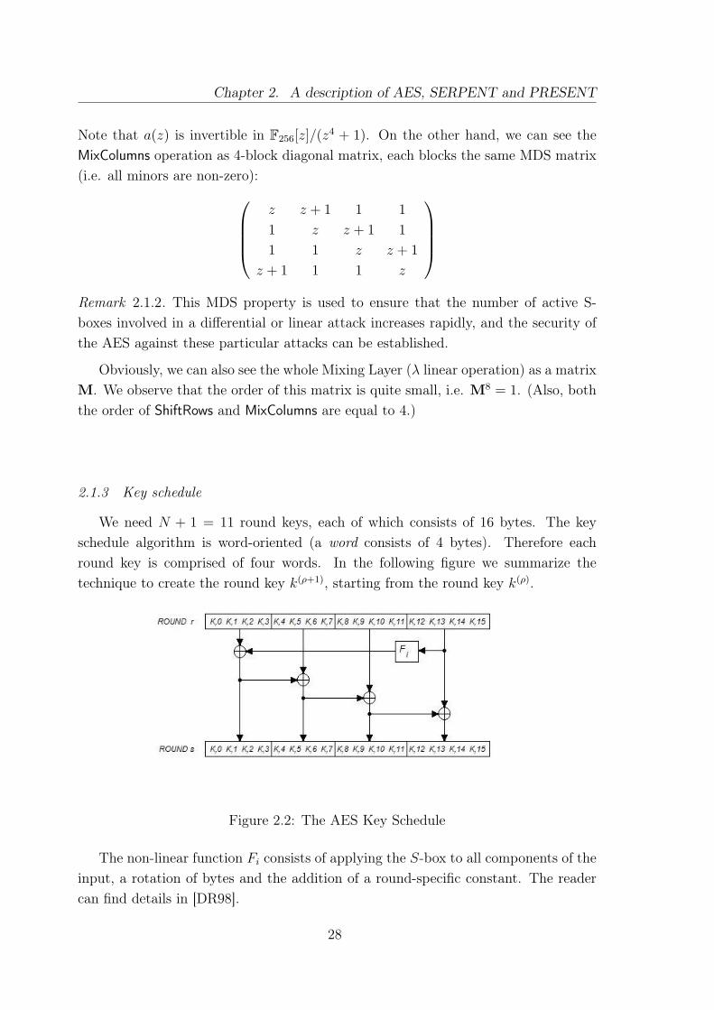
We need N + 1 = 11 round keys, each of which consists of 16 bytes. The keyschedule algorithm is word-oriented (a word consists of 4 bytes). Therefore eachround key is comprised of four words. In the following figure we summarize thetechnique to create the round key k(ρ+1), starting from the round key k(ρ).
Figure 2.2: The AES Key Schedule
The non-linear function Fi consists of applying the S-box to all components of theinput, a rotation of bytes and the addition of a round-specific constant. The readercan find details in [DR98].
28
2.1. The AES cryptosystem
2.1.4 Small scale variants of the AES
For most methods of cryptanalysis it is quite straightforward to perform experi-ments on reduced versions of the cipher to understand how the attack might perform.For new algebraic methods (see Chapter 3.3) it is difficult to design small scale ver-sions that can replicate the main cryptographic and algebraic properties of the cipher.Still, experiments on small versions can give an idea about the behavior of algebraiccryptanalysis on block ciphers.
A family of small scale variants of the AES was proposed by Cid, Murphy andRobshaw in [CMR05]. They define two sets of small scale variants of the AES; theydiffer in the form of the final round. These two sets of variants will be denotedby SR(N, r, c, e) and SR′(N, r, c, e). Both SR(N, r, c, e) and SR′(N, r, c, e) have thefollowing parameters:
• N is the number of (encryption) rounds, 1 ≤ N ≤ 10;
• r is the number of rows in the rectangular arrangement of the input, r = 1, 2, 4;
• c is the number of columns in the rectangular arrangement of the input,c = 1, 2, 4;
• e is the size (in bits) of a word, e = 4, 8.
Both SR(N, r, c, e) and SR′(N, r, c, e) have N rounds and a block size of rce bits,where a data block is viewed as an array of (r × c) words of e bits. The full AES isequivalent to SR′(10, 4, 4, 8).
A round of the small scale variants of the AES consists of small scale variants ofthese operations. For the last round of the AES, the operation MixColumns is omit-ted. Similarly, for SR′(N, r, c, e) the final round does not use MixColumns, whereasMixColumns is retained for the final round of SR(N, r, c, e). The AES is thus identicalto SR′(10, 4, 4, 8).Note that the two ciphertexts produced by SR(N, r, c, e) and SR′(N, r, c, e) when en-crypting the same plaintext under the same key are related by an affine mapping. Asolution of the system of equations for one cipher would immediately give a solutionfor the other and so, without loss of generality, we can only consider SR(N, r, c, e).
29
Chapter 2. A description of AES, SERPENT and PRESENT
2.2 The SERPENT cryptosystem
SERPENT is a translation-based cryptosystem, like AES.Let M = V = (F2)r, with r = 128. We consider K = (F2)`, with the fixed length` = 128, although the key is designed with variable length.The encryption φ proceeds by N = 32 similar rounds and it works as follows:
• a preliminary permutation is applied π : V → V (this is not used for security,rather to ease the implementation);
• there is a preliminary translation with the first round key;
• N − 1 rounds with the same structure are applied, but using a different permu-tation, each composed of a key translation σk, a parallel S-box γ and a linearmixing-layer λ (we denote the round ρ by Round ρ, with ρ = 1, ..., 31);
• the last round (Round 32) follows and it consists of the composition γλσk whereλ = 1V ;
• a final permutation π−1 : V → V is performed.
The decryption process is easily obtained by inverting every step of the encryp-tion, using the inverse of the S-boxes, the inverse of the mixing-layer and the reverseorder of the round keys.
2.2.1 A SERPENT round
Let ρ be a natural number such that 1 ≤ ρ ≤ 31. In order to describe a typicalround (Round ρ) we have to specify how the components γ, λ and σk are applied. Wenote that, after the permutation π : V → V , we perform a preliminary translationσk(0) , where k(0) ∈ (F2)r is the first round key.Let V = V1⊕· · ·⊕V32, where , for any 1 ≤ j ≤ 32, each Vj = (F2)4. Any γ ∈ Sym(V )
acts as vγ = v1γ1 ⊕ . . . ⊕ v32γ32, where vj ∈ Vj and γj ∈ Sym(Vj). We have tocharacterize each γj (i.e. we have to construct each S-box).
The S-boxes of SERPENT were built “ad hoc” starting from the 8 fixed S-boxesof DES (see Appendix) as follows. They were generated using a matrix with 32 arrayseach with 16 entries. The matrix was initialized with the 32 rows of the DES S-boxesand transformed by swapping the entries in the r-th array depending both on thevalue of the entries in the (r+ 1)-st array and on an initial string representing a key.If the resulting array had some desired (differential and linear) properties, the arraywas saved as a SERPENT S-box. The procedure was repeated until the eight S-boxesS1, . . . , S8 have been generated.
30

2.2. The SERPENT cryptosystem
To each vj we apply the same Si mod 8 S-box, so that Si mod 8(vj) lies in (F2)4.That is, γ1 = γ2 = · · · = γ32 = Si mod 8.
Then the linear transformation λ (described in the Subsection 2.2.2) and a finaltranslation σk(ρ) are applied.
The last round (Round 32) is only slightly different. The only difference with atypical round is the replacing of a linear transformation λ by 1V .
π(plaintext)
. . .
π−1(ciphertext)
k(0)
k(1)
k(31)
k(32)
add Round Key
parallel S-box
MixingLayer
add Round key
parallel S-box
MixingLayer
add Round key
parallel S-box
add Round key
2.2.2 The Linear transformation
The linear transformation occurs in each typical round (1 ≤ i ≤ 31) and works onv ∈ V , where V is a direct sum V = V1 ⊕ · · · ⊕ V4 with Vj = (F2)32 (1 ≤ j ≤ 4), insuch a way that the input vector at the i-th round is v = v1 ⊕ v2 ⊕ v3 ⊕ v4.Starting by the initial State (v1, v2, v3, v4), λ the linear transformation is character-ized by the following operations3:
• we sum to v2 the rotat13(v1) and rotat3(v3), obtaining State 1:
(v11, v
12, v
13, v
14) = (rotat13(v1), v2 + rotat13(v1) + rotat3(v3), rotat3(v3), v4);
• we sum to v14 the shift3(v1
1) and v13, obtaining State 2:
(v21, v
22, v
23, v
24) = (v1
1, v12, v
13, shift3(v1
1) + v13 + v1
4);
3rotat denotes a rotation of the bits and shift denotes a bit shift toward the right
31

Chapter 2. A description of AES, SERPENT and PRESENT
• we sum to v21 the rotat1(v2
2) and rotat7(v24), obtaining State 3:
(v31, v
32, v
33, v
34) = (v2
1 + rotat1(v22) + rotat7(v2
4), rotat1(v22), v2
3, rotat7(v24));
• we sum to v33 the shift7(v3
2) and v34, obtaining State 4:
(v41, v
42, v
43, v
44) = (v3
1, v22, shift7(v3
2) + v33 + v3
4, v34);
• we consider the rotat5(v1) and the rotat22(v3), obtaining State 5:
(v51, v
52, v
53, v
54) = (rotat5(v4
1), v42, rotat22(v4
3), v44).
Figure 2.3: Linear transformation of SERPENT
2.2.3 The SERPENT’s key schedule
The round keys of the SERPENT cipher are constructed starting from suitable“prekeys” (w1, . . . , w131) ( for details about the “prekeys” construction, see [BAK98]).Then the authors use the S-boxes to transform the prekeys wi into words ki of theround key by dividing the vector of prekeys into 4 section and transforming the i-thwords of each of the 4 sections using S(r+3−i) mod r. In case r = 32, we have
k0, k33, k66, k99 = S3(w0, w33, w66, w99)
k1, k34, k67, k100 = S2(w1, w34, w67, w100)...
k31, k64, k97, k130 = S4(w31, w64, w97, w130)
k32, k65, k98, k131 = S3(w32, w65, w98, w131).
Then, the 32-bit values kj are renumbered as 128-bit subkeys Ki, (0 ≤ i ≤ r), asfollows Ki = k4i, k4i+1, k4i+2, k4i+3.
32

2.3. PRESENT: an ultra-lightweight block cipher
2.3 PRESENT: an ultra-lightweight block cipher
PRESENT is an iterated block cipher that consists of N = 31 rounds.LetM = V = (F2)r with r = 64. Let K = (F2)`, where ` may be equal to 80 or 128.We consider only the PRESENT’s version such that K = (F2)80, since its authorsrecommend it in order to have a good performance.We are going to describe how the round function γλσk(ρ) (in the ρ-th typical round)is performed.As in the AES and SERPENT cryptosystems, the encryption process starts witha preliminary round (Round 0) that consists of a parallel map γ = 1V , a lineartransformation λ = 1V and the translation σk(0) , where k(0) ∈ (F2)r is the first roundkey. A typical round consists of the non-linear operation, called sBoxLayer, the lineartransformation, known as pLayer and the sum with the round key.
2.3.1 sBoxLayer
The parallel map γ ∈ Sym(V ) used in PRESENT acts as vγ = v1γ1⊕ . . .⊕v16γ16,where each vi ∈ (F2)4 and γi ∈ Sym((F2)4) (1 ≤ i ≤ 16). The action of any brickγi : (F2)4 → (F2)4 is given by the following table, using an hexadecimal notation:
x 0 1 2 3 4 5 6 7 8 9 A B C D E F
γ[x] C 5 6 B 9 0 A D 3 E F 8 4 7 1 2
2.3.2 pLayer
The affine map λ : V → V is a bit permutation as given by the following table,where the bit i of the intermediate state is moved to the bit position P (i).
i 0 1 2 3 4 5 6 7 8 9 10 11 12 13 14 15
P (i) 0 16 32 48 1 17 33 49 2 18 34 50 3 19 35 51
i 16 17 18 19 20 21 22 23 24 25 26 27 28 29 30 31
P (i) 4 20 36 52 5 21 37 53 6 22 38 54 7 23 39 55
i 32 33 34 35 36 37 38 39 40 41 42 43 44 45 46 47
P (i) 8 24 40 56 9 25 41 57 10 26 42 58 11 27 43 59
i 48 49 50 51 52 53 54 55 56 57 58 59 60 61 62 63
P (i) 12 28 44 60 13 29 45 61 14 30 46 62 15 31 47 63
33
Chapter 2. A description of AES, SERPENT and PRESENT
The key schedule
PRESENT supports keys of either 80 or 128 bits. However, we focus on theversion with 80-bit keys. A further useful key is stored in key register K and it isrepresented as K79K78 . . . K0. The ρ-th round key consists of the 64 leftmost bits ofthe current content of the key register K, i.e. k(ρ) = K63K62 . . . K0 = K79K78 . . . K16.After extracting the round key k(ρ), the key register K = K79K78 . . . k0 has to beupdate. The updating procedure occurs in this way:
1. [K79K78 . . . K1K0] = [K18K17 . . . K20K19]
2. [K79K78K77K76] = γi[K79K78K77K76]
3. [K19K18K17K16K15] = [K19K18K17K16K15]⊕ cr
where cr is a round-counter. Thus, the key register is rotated by 61 bit positionsto the left, the left-most four bits are passed through the present S-box, and theround-counter value ρ is exclusive xored with bits K19K18K17K16K15 of K with theleast significant bit of cr on the right.
34
On the AES cryptanalysis
In this chapter we give an overview of the known attacks, especially when appliedto the AES cryptosystem. In Section 3.1 we recall that AES is optimized to resistall known statistical attack. In Section 3.2 we describe some of the structural attacksthat are relevant in the cryptanalysis of reduced variants of AES-128. In Section3.3, Section 3.4, and Section 3.5, we see how the algebraic attacks could be usefulfor a cryptanalyst and we point out some of the alternative representations proposedfor the AES. In particular, we explain the BES representation and the Dual Cipher.Finally, in Section 3.6 we give a sketch of an approach based on changing the S-boxes.
3.1 Statistical attacks
Differential and Linear cryptanalysis are two conventional methods of attackagainst block ciphers. They attempt to construct statistical patterns via many en-cryptions, in order to distinguish the cipher from a random permutation and getthe key. In the Differential cryptanalysis, the statistical pattern depends on bitwisedifferences, instead in Linear cryptanalysis it depends on the correlation among bits.
Linear cryptanalysis, described by Matsui in [Mat93], is a known-plaintext attack.It requires to find a set of linear approximations of the S-boxes that can be used toderive a linear approximation of the whole cipher. The S-boxes used in the approx-imations are called active S-boxes. Suppose that it is possible to find a probabilisticlinear relationship between a subset of plaintext-bits and a subset of state-bits im-mediately preceding the substitutions performed in the last round. We assume thatEve has a large number of (plaintext, ciphertext) pairs encrypted using the same un-known key k. For each of the (plaintext, ciphertext) pairs, we will begin to decryptthe ciphertext, using all possible candidate keys for the last round of the cipher. Foreach candidate pair, we compute the values, of the relevant state-bits involved in thelinear relationship and determine if the above mentioned linear relationship holds.Whenever it does, we increment a counter corresponding to a particular “candidatekey”. At the end of this process, we hope that the candidate key with a frequencycount furthest from half times the number of pairs contains the correct values forthese key bits.
35
Chapter 3. On the AES cryptanalysis
Differential cryptanalysis is a chosen-plaintext attack and was described by Bihamand Shamir in [BS93]. The main difference from the linear cryptanalysis is that itinvolves comparing the XOR of two inputs to the XOR of the corresponding twooutputs. Eve encrypts pairs of plaintexts and studies the propagation of differencesbetween inputs of rounds of the cipher. We assume that Eve has a large numberof tuples (P, P ′, Q,Q′), where the value P ⊕ P ′ is fixed. The plaintext elements Pand P ′ are encrypted using the same unknown key yielding the cyphertexts Q andQ′ respectively. For each of these tuples, we will begin to decrypt the correspondingciphertexts using all possible candidate keys for the last round of the cipher. For eachcandidate keys, we compute the values of certain state bits and determine if theirXOR has a certain value. Whenever it does, we increment a counter corresponding tothe particular candidate key. At the end of this process, we hope that the candidatekey having the highest frequency count contains the correct values for these bits.The Differential cryptanalysis is thwarted by
• careful S-box construction: the probability p of a given bitwise non-zero differ-ence propagation across an S-box is < 2−6, for DES;
• carefully designed diffusion layer.
The total differential probability behaves as pn; attack requirements are proportionalto 1/pn.
The AES cryptosystem is very resistant to these statistical attacks. For differentialand linear cryptanalysis, attacks over 4 rounds of the AES require at least 25 activeS-boxes. More careful analysis takes account of additional complicated phenomena.Exploiting differential and linear techniques requires a massive number of (plaintext,ciphertext) pairs and the complexity usually grows exponentially with the numberof rounds, ensuring that such attacks rapidly become impractical, and so a differentcryptanalytic approach is required.
3.1.1 Distinguishing Attacks
Statistical tools have usually been used with cryptanalytic attacks against blockciphers. Statistical hypothesis testing is a formal way for distinguishing betweentwo probability distributions. Starting from some samples coming from these twodistributions, it is possible to compute the probability that the two distributionsdiffer. In particular, a distinguishing attack on a cipher C relates to the formal modelof security, where an adversary can distinguish between the output of C (with a fixedkey) and the output of a random process, with significant certainty.
Distinguishing attack against block ciphers aim at determining whether a permu-tation corresponds to a permutation chosen uniformly at random from the set of all
36
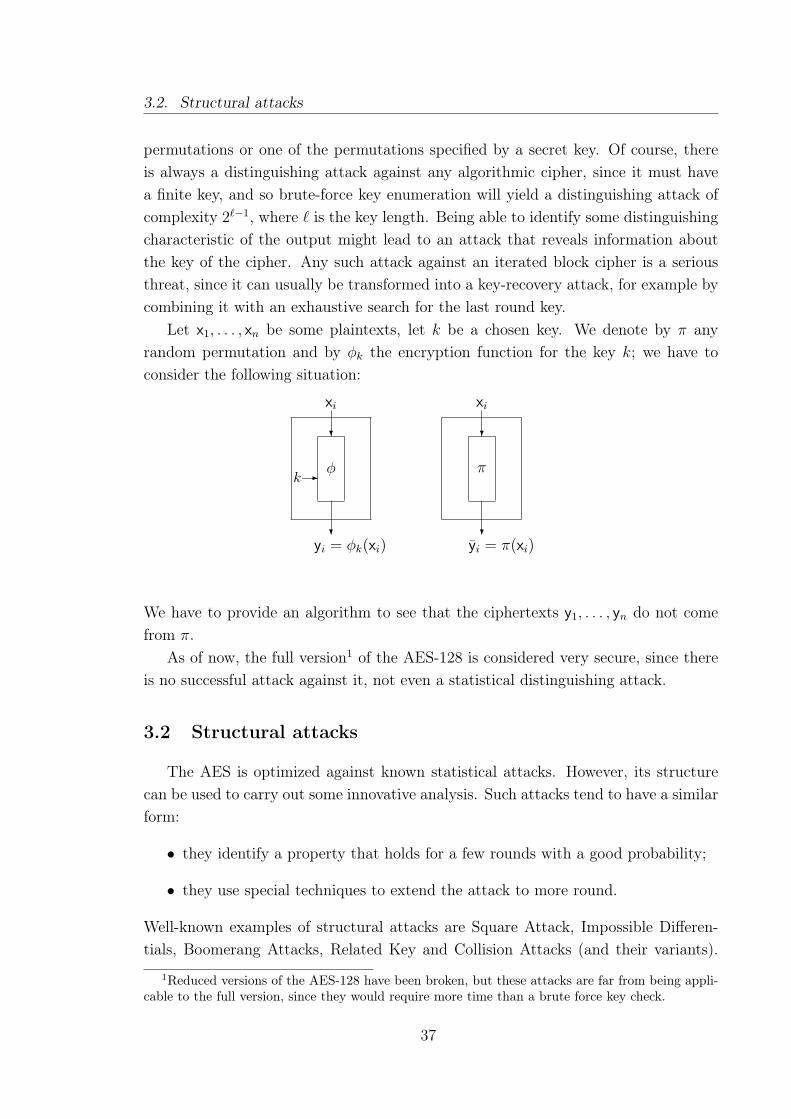
3.2. Structural attacks
permutations or one of the permutations specified by a secret key. Of course, thereis always a distinguishing attack against any algorithmic cipher, since it must havea finite key, and so brute-force key enumeration will yield a distinguishing attack ofcomplexity 2`−1, where ` is the key length. Being able to identify some distinguishingcharacteristic of the output might lead to an attack that reveals information aboutthe key of the cipher. Any such attack against an iterated block cipher is a seriousthreat, since it can usually be transformed into a key-recovery attack, for example bycombining it with an exhaustive search for the last round key.
Let x1, . . . , xn be some plaintexts, let k be a chosen key. We denote by π anyrandom permutation and by φk the encryption function for the key k; we have toconsider the following situation:
φ
?
xi
?yi = φk(xi)
k - π
?
xi
?yi = π(xi)
We have to provide an algorithm to see that the ciphertexts y1, . . . , yn do not comefrom π.
As of now, the full version1 of the AES-128 is considered very secure, since thereis no successful attack against it, not even a statistical distinguishing attack.
3.2 Structural attacks
The AES is optimized against known statistical attacks. However, its structurecan be used to carry out some innovative analysis. Such attacks tend to have a similarform:
• they identify a property that holds for a few rounds with a good probability;
• they use special techniques to extend the attack to more round.
Well-known examples of structural attacks are Square Attack, Impossible Differen-tials, Boomerang Attacks, Related Key and Collision Attacks (and their variants).
1Reduced versions of the AES-128 have been broken, but these attacks are far from being appli-cable to the full version, since they would require more time than a brute force key check.
37

Chapter 3. On the AES cryptanalysis
The following table summarizes the more successful attacks on reduced versions ofthe AES cryptosystem:
Key Rounds Texts Time Type Reference
128 5 211 240 Square attack [DR98]128 5 229.5 231 Impossible diff. [BK00]128 5 239 239 Boomerang attack [Wag99]128 6 232 272 Square attack [DR98]128 6 234.6 244 Partial Sum [FKL+00]128 6 291.5 2122 Impossible diff. [CKK+01]128 6 271 271 Boomerang attack [Wag99]128 7 2128 − 2119 2120 Partial Sum [FKL+00]128 7 232 2128 Collision [GM00]192 7 292 2186 Impossible diff. [Pha04]192 8 2127 2188 Partial Sum [FKL+00]192 10 2124 2183 (Related-key) Rectangle [BDK05]192 12 2123 2176 (Related-key) Ampl. Boomerang [BK09]256 7 292.5 2250.5 Impossible diff. [Pha04]256 8 232 2194 Partial Sum [FKL+00]256 9 285 2126 Partial Sum [FKL+00]256 10 2114 2173 (Related-key) Rectangle [BDK05]256 14 2119 2119 (Related-key) Boomerang [BK09]
3.2.1 Square attack
This is a chosen-plaintext attack that works on any cipher with a round structuresimilar to that of AES. It was first described in the paper presenting a predecessor ofAES, the block cipher Square [DKR97]. For this reason, it is usually called “Square”attack. Other names for this attack are Saturation attack and Integral attack orStructural attack. The original Square attack is able to break reduced variants ofAES up to 6 or 7 rounds faster than exhaustive key search. In 2000 Ferguson et al.[FKL+00] proposed some optimizations that reduce the work factor of the attack. Inthis way, this attack can break up to 9-round of the AES-256 keys with 277 plaintextsunder 256 related keys and 2224 encryptions.
In order to describe the 6-round Square Attack, we first explain the basic attackon 4 rounds and then we will show how Deamen and Rijmen extended it to the 5-thand the 6-th rounds in their original proposal [DR98]. This attack is independent ofthe specific choices of SubBytes, the multiplication polynomial of MixColumns and theKey Schedule and works against all block sizes and key sizes.
38

3.2. Structural attacks
Consider a set in which only one byte is active, that is, we change the value ofone bytes only. We can see the following situation
• MixColumns of the 1st round converts the active byte to a complete column ofactive bytes.
Figure 3.1: Square attack, first round
• The four active bytes of this column are spread over four distinct columns byShiftRows of the 2nd round.
• MixColumns of the 2nd round subsequently converts this to 4 columns of onlyactive bytes.
Figure 3.2: Square Attack, second round
• Although at the end of the second round all bytes potentially change, we arestill able to recover the first byte by solving a linear system. This is not possibleany more after the input of MixColumns of the 3rd round.
Figure 3.3: Square Attack, third round
39

Chapter 3. On the AES cryptanalysis
We use m(ρ), b(ρ), and t(ρ) to refer to intermediate text values used in round ρ
after the MixColumns, key addition, and ShiftRows operations, respectively. We writek(ρ) for the subkey in round ρ , and k(ρ)′ for an equivalent subkey value that may bexored into the state before (instead of after) the MixColumns operation in round ρ .The idea is to choose a set of plaintexts that results in a set at the output of the 1stround with a single active S-box. This requires the assumption of values of four bytesof the Round Key that is applied before the first round.If the intermediate state after MixColumns of the first round has only a single activebyte, this is also the case for the input of the second round. This imposes the followingconditions on a column of 4 input bytes of MixColumns of the second round: oneparticular linear combination of these bytes must range over all 256 possible values(active) while 3 other particular linear combinations must be constant for all 256
states. This imposes identical conditions on 4 bytes, in different positions at theinput of ShiftRows of the first round. If the corresponding bytes of the first round keyare known, these conditions can be converted to conditions on 4 plaintext bytes.Now we consider a set of 232 plaintexts, such that one column of bytes at the inputof MixColumns of the first round ranges over all possible values and all other bytesare constant. Now, an assumption is made for the value of the 4 bytes of the relevantbytes of the first Round Key. From the set of 232 available plaintexts, a set of 256
plaintexts can be selected that result in a set at the input of round 2. Now the 4-round attack can be performed.For the given key assumption, the attack can be repeated for several plaintext sets.If the byte values of the last Round Key are not consistent, the initial assumptionmust have been wrong. A correct assumption for the 32 bytes of the first Round Keywill result in the swift and consistent recuperation of the last Round Key.
3.2.2 Partial Sum
The attack of previous section on 4 rounds of AES can be improved. Instead ofguessing four bytes of k(0) we simply use all 232 plaintexts.For any value of the first round key, these encryptions consist of 224 groups of 28
encryptions that vary only in a single byte of the output of the MixColumns operationat first round. All we have to do is to guess the five key bytes at the end of thecipher, do a partial decrypt to a single byte of b(4), sum this value over all the 232
encryptions, and check for a zero result. Compared to the original version, we guessonly 40 bits of key instead of 72. On the other hand, we have to do 224 times as muchwork for each guess. All in all, this improvement reduces the workload by a factor of28, although it needs about 6 · 232 plaintexts to provide enough sets of 232 plaintextsto uniquely identify the proper value for the five key bytes.
40
3.2. Structural attacks
We will now look at this attack in more detail.We have 232 ciphertexts. We guess five key bytes, do a partial decryption from eachof the ciphertexts to a single byte in b(4), and sum this byte over all ciphertexts.Consider this partial decryption. From any ciphertext, we use four ciphertext bytes.Each of these is xored with a key byte. We then apply the inverse S-box to each byte,and multiply each with an appropriate factor from the inverse MDS matrix. The fourbytes are then xored together, a fifth key byte is xored into the result, the inverseS-box is applied, and the resulting value is summed over all ciphertexts.Let ci,j be the j-th byte of the i−th ciphertext. (We leave out the i subscript if weare not talking about any particular ciphertext.) For simplicity we will number thefour bytes of each ciphertext that we use from 0 to 3.Let k0, . . . , k4 denote the five key bytes that we are guessing. We want to computethe following∑
i
S−1[S0[ci,0 ⊕ k0]⊕ S1[ci,1 ⊕ k1]⊕ S2[ci,2 ⊕ k2]⊕ S3[ci,3 ⊕ k3]⊕ k4]
where S0, . . . , S3 are bijective S-boxes, each of which consists of an inverse AES S-box followed by a multiplication by a field element from the inverse MDS matrix.Given 232 ciphertexts and 240 possible key guesses, we have to sum 272 different values,which corresponds roughly in amount of work to doing about 264 trial encryptions.We can organize this more efficiently in the following manner. For each k, we associatea “partial sum” xk to each ciphertext c, defined as follows:
xk :=k∑j=0
Sj[cj ⊕ kj]
This gives us a map (c0, c1, c2, c3) 7→ (xk, ck+1, . . . , c3) that we can apply to each ci-phertext if we know k0, . . . , kk.We start out with a list of 232 ciphertexts. We guess k0 and k1 and compute how ofteneach triple (x1, c2, c3) occurs in the list. That is, for each i, we compute the three-bytevalue (S0[ci,0 ⊕ k0]⊕ S1[ci,1 ⊕ k1], ci,2, ci3) as a function of the i-th ciphertext and theguessed key material, and we count how many times each three-byte value appearsduring this computation. As there are only 224 possible values for three bytes, we donot have to list all (x1, c2, c3) values; rather, we count how often each triple occurs.We then guess k2 and compute how often each tuple (x2, c3) occurs; and guess k3
and compute how often each value of x3 occurs. Finally, we guess k4 and computethe desired sum. Because all sums are taken using the XOR operation (and becausez ⊕ z = 0 for all z), it suffices to only count modulo two. Thus, a single bit sufficesfor each count, and so the space requirement for the 224 counters is just 224 bits.
41

Chapter 3. On the AES cryptanalysis
How much work has this been? In the first phase we guessed 16 bits and processed232 ciphertexts, so this phase costs 248 overall. In the next phase, we guessed a totalof 24 bits but we only had to process 224 triples, so this costs 248 as well. This holdssimilarly for each of the phases. In total, the entire computation requires the equiv-alent of about 248 evaluations of equation 1, or about 250 S-box applications.This is the amount of work required for a single structure of 232 ciphertexts. The firststructure already weeds out the overwhelming majority of the wrong key guesses, butwe still have to do the first steps of our partial sum computation for each of the sixstructures that we use. The total number of S-box lookups is thus about 252.Using our earlier rough equivalence of 28 S-box applications to a trial encryption witha new key, the 252 S-box applications are comparable to 244 trial encryptions. This isa significant improvement over the earlier 272 work factor.
Remark 3.2.1. We can extend the previous approach to the 7-round version of thisattack. To express a single byte of b(4) in the key and the ciphertext, we get a formulasimilar to equation 1 but with three levels, 16 ciphertext bytes, and 21 key bytes. Thepartial sum technique is only helpful during the last part of the computation as itonly saves work if there are more ciphertexts than possible values for the intermediateresult. With 232 plaintext/ciphertext pairs in a structure, these techniques will nothelp until the very last part of the computation.
3.2.3 Impossible Differentials
There exists an impossible differential attack on 5 rounds [BK00], requiring 229.5
chosen plaintext, 231 encryptions, 242 bytes of memory and 226 time for pre-computation.This result was improved and lead to an attack on a 6 round version [CKK+01].
3.2.4 Collision Attacks
This attack has been introduced by Gilbert and Minier in [GM00] and is still thebest attack in the sense that it can break 7 rounds of AES-128, AES-192 and AES-256. For AES-128 the authors claim that the complexity of the attack is marginallylower than the complexity of an exhaustive key search.
3.2.5 Boomerang attack
The Boomerang attack is an “adaptive chosen-plaintext” and “adaptive chosen-ciphertext” attack (see Section 1.2.3) and was introduced by Wagner in [Wag99].This attack is based on two differentials. The main problem consists of finding “good”differentials. Suppose we have a block cipher φ : 0, 1r ×0, 1` → 0, 1r for which
42

3.2. Structural attacks
we know that an input difference α induces an output difference β with probabilityp. We use this property to retrieve the round key both in the cipher itself, or if weare dealing with part of the cipher, in the rounds before and after the part for whichwe have a differential. This kind of work is less effective against ciphers where theprobability of the next differential drops very fast with the number of rounds: AESand SERPENT are such two examples. In the AES cryptosystem there are 1-rounddifferentials with probability 2−7 and 2-round differentials with probability 2−35. Theprobability of the best differential drops faster than exponentially with the numberof rounds. In particular, it can be shown that the best 4-round differential for AEShas probability no more than 2−96.
Sketch of the attack
Let us assume that the encryption function φ is a composition of two parts: φ0
and φ1. Suppose to have a good differential in φ0 : α → β with probability p andanother good differential in φ1 : γ → δ with probability q.As mentioned before, it is easy to find such short differentials (for parts of the cipher),but we need to find long differentials with good probability. The question is thefollowing: how to combine these two differentials to mount an attack against the fullcipher φ?Let us examine the encryption of the plaintexts P1 and P2 = P1 + α through φ0.Starting from the differential we have that φ0(P1) + φ0(P2) = β with probability p.The corresponding ciphertexts are C1 = φ1(φ0(P1)) and C2 = φ1(φ0(P2)).Now we compute C1 +δ = C3 and C2 +δ = C4. When we partially decrypt the valuesof C1 and C3 though φ1, we know that
φ−11 (C1) + φ−1
1 (C3) = γ
with probability q. The same holds for C2 and C4:
φ−11 (C2) + φ−1
1 (C4) = γ.
Since φ0(P1) = φ−11 (C1) and φ0(P2) = φ−1
1 (C2), using the previous equalities, we have
φ0(P1) + φ−11 (C3) = φ0(P2) + φ−1
1 (C4)
φ0(P1) + φ0(P2) = φ−11 (C3) + φ−1
1 (C4)
β = φ−11 (C3) + φ−1
1 (C4)
Hence, if we continue the decryption process, we get P3 +P4 = α with probability q2.Under the above assumptions, we say that both (P1, P2) and (P3, P4) are right pairsfor the characteristic α → β and that (C1, C2) and (C3, C4) are right pairs for the
43
Chapter 3. On the AES cryptanalysis
characteristic γ → δ. Then, we can use these for retrieving the subkeys in φ0 and φ1
similarly to differential cryptanalysis. The probability for such a quartet to be rightis 2−n.
The Amplified Boomerang attack
Kohno, Kelsey and Scheneir [KKS00] introduced the Amplified Boomerang At-tack. This method converts the Adaptive Chosen Plaintext and Ciphertext into aChosen Plaintext attack. This is done by encrypting many plaintexts pairs with in-put difference α. If we start with N plaintext pairs (P, P + α), then about Np ofthose pairs will have a difference β after φ0.With probability 2−n the difference between the intermediate encryption value of P1
and P3 is γ. If this is the case, then the difference between the intermediate encryp-tion values of P2 and P4 is also γ. Then, with probability q for each of these pairs,we get that the corresponding ciphertexts pairs have difference δ.Hence, out of the N pairs we started with, we get 2−np2q2N2/2 quadruplets.
The Rectangle attack
The amplified boomerang attack has a major drawback: one needs to check all pos-sible quadruplets to find the right quadruplets. Unlike the boomerang attack, wherewe know exactly what plaintexts we need to compare, in the amplified boomerangattack, we have no idea about the quadruplets that we need to check.Another drawback is the very low probability of a quadruplet to be a right quadru-plet. For example, even if the probabilities of the differentials are 1 (i.e. p = q = 1),in order to obtain one right quadruplet, we still need 2n/2 pairs.Biham, Dunkelman and Keller [BK00] introduced the Rectangle Attack. The at-tack has much higher probability (i.e. the probability of a quadruplet to be a rightquadruplet is higher) and also better attack algorithm (based on more efficient datastructures and attack algorithm).By examining both the pair (C1, C3) and the pair (C2, C4) for a δ difference, the num-ber of right quadruplets is multiplied by 2, (as we check N2 different quadruplets).Moreover it is possible to apply the improvements of the boomerang attack which usemany differentials simultaneously.
Attacks on small scale variants of AES
We describe a generic method of breaking 5 round (using boomerang techniques)of one AES-like cipher. This structural attack does not use specific properties of theS-boxes or the Mixing Layer, but it uses only the fact that diffusion is incomplete.
44

3.2. Structural attacks
We also note that the exact constants in the MixColumns matrix will be irrelevant tothe attack.
• Let Pi, i = 0, . . . , 232 − 1 be a pool of plaintexts which have all possiblevalues in four bytes and arbitrary constants in the other bytes. Encrypt eachPi obtanining a pool of 232 ciphertexts Ci.
• Contruct a pool of modified ciphertexts: Di = Ci ⊕∇, where ∇ is a fixed non-zero difference with only one active S-box. Decrypt the pool Di to obtain apool Qi of 232 new plaintexts.
• Sort the pool Qi by the bytes corresponding to eight inactive S-boxes. Pickonly those pairs Qi, Qj which have zero difference in these 8 bytes. If none isfound we have to come back to the first step.
• For each of the right (according to the previous step) quartets Pi, Pj, Qi, Qj,guess the 32-bit key value that enters the 4 S-boxes corresponding to non-constants bytes. Using the guessed key value, partially encrypt one round andcheck the resulting difference in a single active S-box, which is a 22-bit filteringcondition for each pair (Pi, Pj) and (Qi, Qj). This gives a 44-bit condition intotal for both sides of the boomerang in the case of common 4-tuples to activeS-boxes. However, with half probability we will have no common 4-tuples, i.e.all the 12 active S-boxes (4 from the (Pi, Pj) pairs and 8 from the (Qi, Qj) pairs)do not overlap. We will pick key-candidates that are suggested at least twice.
Remark 3.2.2. The attack described above can be extended by one round to thebottom at the cost of guessing 32-bit of the key of the 6th round.
Figure 3.4: Schematic description for AES reduced to five rounds
45

Chapter 3. On the AES cryptanalysis
3.3 First algebraic attacks
In contrast to conventional block cipher cryptanalysis, algebraic cryptanalysisexploits the intrinsic algebraic structure of a cipher. In its most common form, acryptanalyst describes the encryption transformation as a set of multivariate poly-nomial equations, which once solved can be used to recover information about thesecret key. The algebraic attacks can be briefly sketched as follows:
• Collecting Step: Eve expresses the cipher as a set of “suitable” equations in oneor more variables. These variables may include bits (or bytes) from the plain-text, ciphertext and the key. Typically, the variables include also intermediatecomputation values and round keys.
• Solving Step: Eve uses some data input, such as the pairs (plaintext, ciphertext);she substitutes these input values in the corresponding variables (in the set ofequations collected in the previous step) and tries to solve the resulting set ofequations, thereby recovering the key.
Several attempts have been made to construct algebraic attacks for the AES. Theyhave resulted in small scale variants attacks as yet, and many of the related papersconclude that more research is required. The most important attempts in this senseare the following:
• Ferguson, Shroeppel and Whiting in [FSW01] derive a closed formula for AESthat can be seen as a generalization of continued fractions.
• Courtois and Pieprzyck [CP02] observe that the S-box used in the AES can bedescribed by a number of implicit quadratic Boolean equations.
• Murphy and Robshaw [MR02] define the block cipher BES which operates ondata blocks of 128 bytes instead of bits. According to Murphy and Robshaw,the algebraic structure of BES is even more elegant and simple than that of theAES.
• In 2002 Barkan and Biham [BB02b] introduced the concept of Dual ciphers. Itis basically a generalization of the embedding technique.
46
3.3. First algebraic attacks
3.3.1 Continued fractions
Let us consider a typical round of the AES. We write an algebraic expression ofall the steps:
SubBytes: s(ρ)i,j = S[a
(ρ)i,j ] =
∑7dρ=0wdρ(a
(ρ)i,j )−2dρ
ShiftRows: t(ρ)i,j = s
(ρ)i,i+j
MixColumns: m(ρ)i,j =
∑3eρ=0 vi,eρt
(ρ)eρ,j
AddRoundKey: a(ρ+1)i,j = m
(ρ)i,j + k
(ρ)i,j
where wdρ are suitable constants, a(ρ)i,j is the byte at position (i, j) at the input of
round ρ, vi,j are the coefficients of the MDS matrix and k(ρ)i,j is the ρ-th round key at
position (i, j). Clearly, we can rewrite the last formula in the following way:
a(ρ+1)i,j = k
(ρ)i,j +
∑eρ∈E, dρ∈D
wi,eρ,dρ
(aeρ,eρ+j)2dρ,
where E := 0, . . . 3 and D := 0, . . . 7.What happens after the second round? We get the following expression
a(3)i,j = k
(3)i,j +
∑e2∈E, d2∈D
wi,e2,d2(k
(1)e2,e2+j +
∑e1∈E, d1∈D
we2,e1,d1
(ae1,e1+e2+j)2d1
)2d2
or equivalently, we have
a(3)i,j = k
(3)i,j +
∑e2∈E, d2∈D
wi,e2,d2
(k(1)e2,e2+j)
2d2 +∑
e1∈E, d1∈Dw2d2e2,e1,d1
(ae1,e1+e2+j)2d1+d2
.
Note that all the subscripts are known and they are independent of the key or plain-text. The same holds for all the exponents, that is they are known and independentof the plaintext and key.A fully expanded version of any byte of the intermediate result after 5 rounds has 225
terms. Even the full 10 round formula would require only 250 terms or so, which iscertainly computable within the workload allowed for an attack on a 128-bit cipher.Therefore, the security of AES depends on the following assumption: it is computa-tionally infeasible to solve equations of this type.In order to break the AES cryptosystem, Eve could use two equations of this type foreach intermediate byte. The first one would express the intermediate variables after5 rounds as function of the plaintext bytes. The second equation would cover rounds,from the 6th to the 10th, by expressing the same intermediate variables as a func-tion of the ciphertext bytes. Combining both equations would result in an equation
47

Chapter 3. On the AES cryptanalysis
with 226 unknowns. By repeating this equation for 226/16 known pairs (plaintext,ciphertext), enough information could be gathered to solve for the unknowns, in aninformation-theoretic sense. It is currently unknown what practical algorithm mightsolve this type of equations.
3.3.2 Polynomial system approach
In this subsection we consider the encryption as a set of multivariate polynomialsequations. Once this system is solved, we can use the corresponding solution torecover information about the secret key.
Let φ : (F2)r × (F2)` → (F2)r be the encryption function. The componentsφ1, · · · , φr of φ are polynomials in F2[x1, . . . , xr, k1, . . . , k`].Since we are looking for solutions in F2, we have the following relations
(x1)2 = x1
...(xr)
2 = xr
(k1)2 = k1
...(k`)
2 = k`
We want to apply the Chosen Plaintext attack. Let x ∈M be a plaintext and lety ∈M be the corresponding ciphertext. For any pair (x, y) we have this system
φ1(x, k) = y1
φ2(x, k) = y2
...φr(x, k) = yr
Remark 3.3.1. Note that yi and xi (i = 1, . . . , r) are constants and that the compo-nents of the key k1, . . . , k` are variables.
We denote with εi(k) = φi(k, x) for i = 1, . . . , r. Note that εi is a polynomials inF2[k1, . . . , k`]. We have to solve the following system
ε1(k) = y1
ε2(k) = y2
...εr(k) = yr
(k1)2 = k1
(k2)2 = k2
...(k`)
2 = k`
48

3.3. First algebraic attacks
We overcome the following kinds of Problems:
1. We can describe the encryption function φ but it could be very difficult to findthe components ε1, · · · , εr describing the function as polynomials.
2. Suppose that we know ε1, · · · , εr. The corresponding system can be too denseto be stored on a computer.
3. Even if we can store the system, to solve it could be very difficult (unless it isvery sparse and it has low degree).
How to solve polynomial systems? Well-known techniques to solve a system arethe following:
• explicit substitutions when possible;
• compute Gröbner basis.
A classical general algorithm for computing a Gröbner basis of polynomial ideal isBuchberger’s algorithm ([Buc65], [Buc06]). The F4 and F5 algorithms have beenproposed as alternative approaches for computing Gröbner bases. Since the maincomputational cost of Buchberger’s algorithm lies in polynomial reductions, whichtake place sequentially, the F4 essentially replaces many sequential polynomial re-ductions with a matrix reduction, F5 algorithm permits in addition to detect uselesspolynomial reductions. These algorithms are based on the idea of combining Gröbnerbasis computation with Gaussian elimination and work by performing the multivari-ate division algorithm as a matrix reduction.For AES-128 [BPW06a], a zero-dimensional Gröbner basis for the key-recovery idealcan be constructed with minimal computational effort, without performing a singlepolynomial reduction. This is achieved by constructing a polynomial system in whichall leading terms are pairwise prime, allowing the first Buchberger criterion to be usedto show that the resulting set of polynomials forms a Gröbner basis. The Gröbnerbasis of the key-recovery ideal for AES-128 IAES ∈ RAES [BPW06b] consists of 200
polynomials of degree 254 and 152 linear polynomials in a ring of 352 variables. Thevector space dimension dim(RAES/IAES) unfortunately is 254200, which makes theGröbner basis unsuitable for cryptanalysis.
In the real situations the polynomial approach does not work and one can changethe system representation. In practice, a very efficient solver of sparse polynomialequations over F2 is PolyBori ([pol], [BD07]).
49
Chapter 3. On the AES cryptanalysis
3.4 Alternative representations
Several alternative representations have been proposed for the AES. Let φ be ouroriginal block cipher and φ′ be a new block cipher. We can define a representationmap σ (1-1) and
(Fq)n
φk
σ // (FQ)m
φ′k
(Fq)n σ // (FQ)m
We say that the block cipher φ′ is an alternative representation of the block cipher φif the previous diagram is a commutative diagram.
Murphy and Robshaw defined a new block cipher, the Big Encryption Standard(BES), which operates on data blocks of 128 bytes instead of bits. The algebraicstructure of BES is even simpler than that of AES. Furthermore, the AES can beembedded into BES; indeed there exists a map σ such that
AESK(x) = σ−1(BESσ(K)(σ(x))).
Murphy and Robshaw believed that when the XSL method [CKPS00] is applied toBES, the complexity of the Solving step could be significantly smaller than in the casewhere XSL is directly applied to AES. In [LK07] the authors descussed of the XSLmethod against BES.Toli and Zanoni proved in [TZ05] that Murphy and Robshaw’s system is not complete,because they omitted some indispensable equations and so this reduced-complexity donot work to attack AES. Note that the BES could still be an interesting representation.
3.4.1 BES
The BES cipher, in which AES is embedded using a natural map, involves onlycomputations in F28 . This fact permits to describe AES using some polynomial equa-tion systems. Solving them means to find the key or another variable and thereforeto break the cryptosystem.We denote by A = (F28)16 and B = (F28)128 the state spaces of AES and BES re-spectively. The basic tool for embedding is the conjugation operation σ, taking eightsuccessive square powers, for each value in F28 :
(F28)16
AES
σ // (F28)128
BES
(F28)16 σ // (F28)128
.
50

3.4. Alternative representations
The map σ is defined in the following way
a ∈ F28 7→ σ(a) = (a20
, a21
, . . . , a27
) ∈ (F28)8
a ∈ (F28)n 7→ σ(a) = (σ(a0), . . . , σ(a7)) ∈ (F28)8n
It is easily verified that σ(a + a′) = σ(a) + σ(a′) and σ(a−1) = σ(a)−1 assuming that0−1 = 0. Moreover, we define BA = σ(A) ⊂ B as the subset of B corresponding to A.
Let p, c ∈ B be the plaintext and the ciphertext, respectively; wi,xi ∈ B , where0 ≤ i ≤ 9, the state vectors before and after the inversion phases and hi ∈ B theused key. All the phases of AES algorithm may be translated in B using just linearalgebra in F28 , excepting from inversion, which is done component-wise, as follows.The matrix LA : (F2)8 → (F2)8 for the affine transformation for one byte in theSubBytes operation can be represented by the polynomial function f : F28 → F28 :
f(a) =7∑
k=0
λka2k
with
λ0 = t2 + 1 λ4 = t7 + t6 + t5 + t4 + t2
λ1 = t3 + 1 λ5 = 1
λ2 = t7 + t6 + t5 + t4 + t3 + 1 λ6 = t7 + t5 + t4 + t2 + 1
λ3 = t5 + t2 + 1 λ7 = t7 + t3 + t2 + t+ 1
It is possible to translate this formulation in the B state space as follows
LB(a) = σ(LA(a)) = (f(a)20
, . . . , f(a)27
).
The successive squares of f are needed, and the answer is given by a simple inductionwith basic step
(f(a))2 =( 7∑k=0
λka2k)2
=7∑
k=0
λ2ka
2k·2 =7∑
k=0
λ2ka
2k+1
.
The resulting matrix, which we still indicate with LB, is
LB = [`ij]i,j=0...7 with `ij = λ2i
(8−i+j) mod 8
If we consider the entire transformation LinB : (F28)128 → (F28)128, we obtain a blockdiagonal matrix with 16 blocks equal to LB.
51

Chapter 3. On the AES cryptanalysis
The AES SubBytes constant cA = 63 = t6 + t5 + t+ 1 ∈ F28 maps into
σ(cA) = (63,C2, 35, 66,D3, 2F, 39, 36) = (t6 + t5 + t+ 1, t7 + t6 + t,
t5 + t4 + t2 + 1, t6 + t5 + t2 + 1, t7 + t6 + t4 + t+ 1,
t5 + t3 + t2 + t+ 1, t5 + t4 + t3 + 1, t5 + t4 + t2 + t).
The corresponding BES vector cB is obtained by the juxtaposition of 16 consecutivecopies of σ(cA), cB = σ(cA, . . . , cA) = (σ(cA), . . . , σ(cA)), such that
[cB]i = [σ(cA)]i mod 8.
The AES ShiftRows operation permutes the bytes in the array. Clearly, this processcan be considered as a transformation of the components of a column vector a ∈ A.It is straightforward to represent this transformation as multiplication of the statevector a ∈ A by a 16× 16 (F28)-matrix RA : (F28)16 → (F28)16:
RA =
1 0 0 0 0 0 0 0 0 0 0 0 0 0 0 0
0 0 0 0 0 1 0 0 0 0 0 0 0 0 0 0
0 0 0 0 0 0 0 0 0 0 1 0 0 0 0 0
0 0 0 0 0 0 0 0 0 0 0 0 0 0 0 1
0 0 0 0 1 0 0 0 0 0 0 0 0 0 0 0
0 0 0 0 0 0 0 0 0 1 0 0 0 0 0 0
0 0 0 0 0 0 0 0 0 0 0 0 0 0 1 0
0 0 0 1 0 0 0 0 0 0 0 0 0 0 0 0
0 0 0 0 0 0 0 0 1 0 0 0 0 0 0 0
0 0 0 0 0 0 0 0 0 0 0 0 0 1 0 0
0 0 1 0 0 0 0 0 0 0 0 0 0 0 0 0
0 0 0 0 0 0 0 1 0 0 0 0 0 0 0 0
0 0 0 0 0 0 0 0 0 0 0 0 1 0 0 0
0 1 0 0 0 0 0 0 0 0 0 0 0 0 0 0
0 0 0 0 0 0 1 0 0 0 0 0 0 0 0 0
0 0 0 0 0 0 0 0 0 0 0 1 0 0 0 0
The corresponding BES matrix is obtained by expanding each 1 in RA with an identitymatrix of the order 8 and each 0 with a zero (8 × 8)-matrix. The result will beRB : (F28)128 → (F28)128. Moving from RA to RB we only need to ensure that thevector conjugates are moved as a single entity.
52

3.4. Alternative representations
The AESMixColumnsmay be represented using the following CA : (F28)4 → (F28)4
CA =
t t+ 1 1 1
1 t t+ 1 1
1 1 t t+ 1
t+ 1 1 1 t
The AES transformation is given by the MixA : (F28)16 → (F28)16 block diagonal
matrix having as blocks four copies of CA. In order to obtain the correspondingmatrix, we first need to compute the following matrices CB
(k), for k = 0, . . . , 7:
C(k)B =
t2k
(t+ 1)2k 1 1
1 t2k
(t+ 1)2k 1
1 1 t2k
(t+ 1)2k
(t+ 1)2k 1 1 t2k
with
t20
= t t24
= t6 + t4 + t3 + t2 + t
t21
= t2 t25
= t7 + t6 + t5 + t2
t22
= t4 t26
= t6 + t3 + t2 + 1
t23
= t4 + t3 + t+ 1 t27
= t7 + t6 + t5 + t4 + t3 + t
from which (t+ 1)2k = t2k
+ 1 may be very easily computed.Using an appropriate basis, the resulting matrix MB : (F28)128 → (F28)128 may bewritten as a block diagonal one, with four consecutive copies of CB
(k) for all possiblek. The different position of value powers in σ’s image, with respect to our needs,makes the change of basis necessary. Indeed, if a ∈ (F28)16, then
σ(a) = (a0, . . . , a27
0 , a1, . . . , a27
1 , . . . , a15, . . . , a27
15),
while in order to use the block diagonal representation, we would need the followingvector:
a′ = (a0, . . . , a15, a20, . . . , a
215, . . . , a
27
0 , . . . , a27
15).
This transformation is given by a permutation matrix PermB : (F28)128 → (F28)128.To represent it easily, suppose to divide it into (16×8) sub-matrices Phk, h = 0, . . . , 7
and k = 0, . . . , 15. Each sub-matrix element (with i = 0, . . . , 15 and j = 0, . . . , 7) is :
[Phk]ij =
1 if i = k and j = h
0 else
53
Chapter 3. On the AES cryptanalysis
Key schedule: we can use the same techniques from previous sections to describe thekey schedule for the BES. In fact the key schedule in the AES uses the same opera-tions as the F2-linear map, component-wise inversion, byte rotation and addition.
Round function of BES: we can write the final formula for the round function forthe BES, supposing that the state at the beginning of the round of the BES is b ∈ B
and the BES round key is kBi ∈ B. We can obtain the following
RoundB(b, (kB)i) = MixB(RB(LinB(b−1) + cB)) + (hB)i
= MB · (b−1) + (CB(cB)(hB)i)
= MB · (b−1) + (kB)i
where
MB = MixB ·RB · LinB, CB = MixB ·RB, (kB)i = CB(cB) + (hB)i.
Note that for the last round, we will have (kB)i = RB(cB) + (hB)i.
3.4.2 Polynomial system
Murphy and Robshaw claimed that recovering an AES key is equivalent to solvingparticular systems of extremely sparse multivariate quadratic equations by expressinga BES (and hence an AES) encryption as such a system. The problem of solving suchsystems of equations lies at the heart of several public key cryptosystems and therehas been some progress in providing solutions to such problems.
Courtois and Pieprzyk have suggested the use of a system of multivariate quadraticequations over F2 to analyze the AES. However, such a F2-system derived directlyfrom the AES is far more complicated than the F28-system derived from the BES.A BES encryption is described by the following system of equation, remembering thatthe last round differs slightly from the other ones, withM∗
B = RB·LinB = Mix−1B ·MB,
w = p + k0
xi = w−1i i = 0, . . . , 9
wi = MBxi−1 + ki i = 1, . . . , 9
c = M∗Bx9 + k10
If we consider the previous equations component wise, let the (8j+m)th componentof all the vectors be indicated using the indexes expression (j,m) with j = 0, . . . 15
and m = 0, . . . 7. Under the hypothesis that no 0-inversion occurs (true for the 53%of encryptions and 85% of 128-bit keys), it is possible to expand the above system as
54
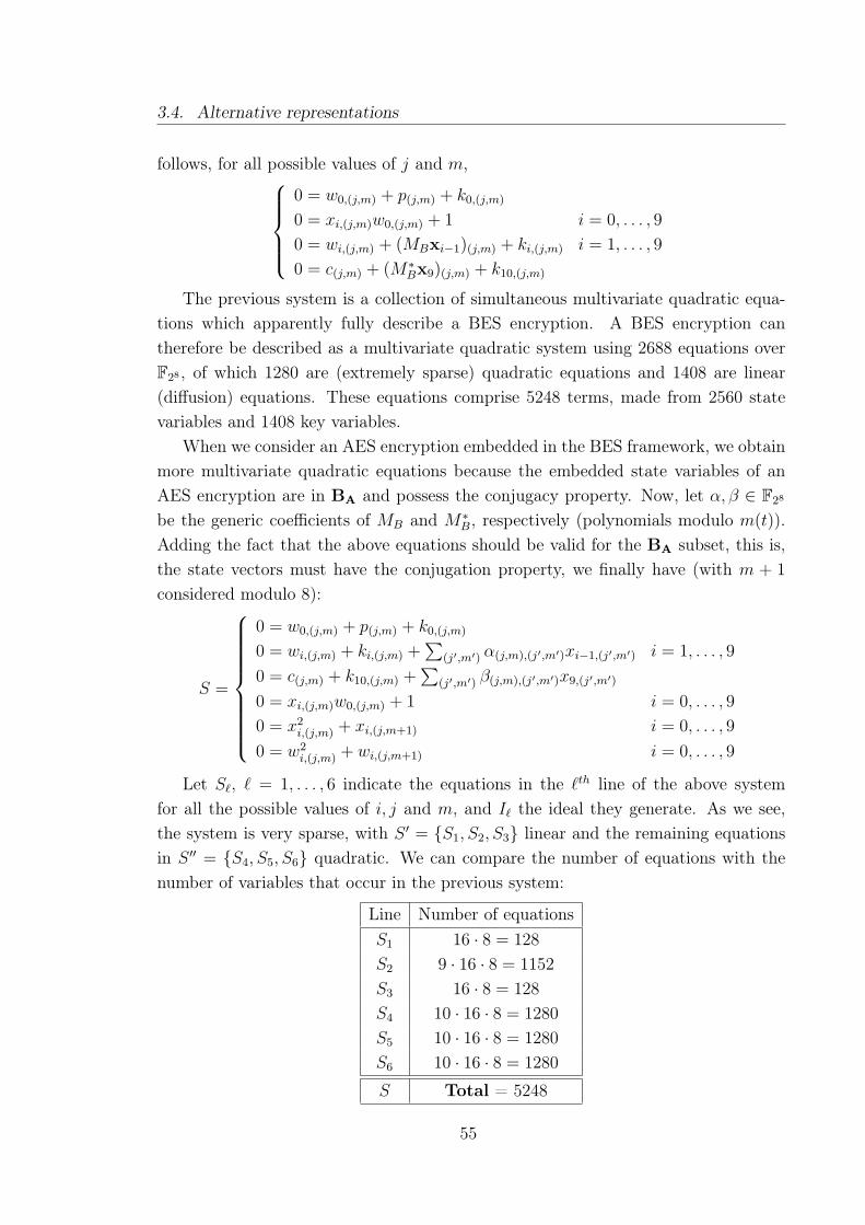
3.4. Alternative representations
follows, for all possible values of j and m,0 = w0,(j,m) + p(j,m) + k0,(j,m)
0 = xi,(j,m)w0,(j,m) + 1 i = 0, . . . , 9
0 = wi,(j,m) + (MBxi−1)(j,m) + ki,(j,m) i = 1, . . . , 9
0 = c(j,m) + (M∗Bx9)(j,m) + k10,(j,m)
The previous system is a collection of simultaneous multivariate quadratic equa-tions which apparently fully describe a BES encryption. A BES encryption cantherefore be described as a multivariate quadratic system using 2688 equations overF28 , of which 1280 are (extremely sparse) quadratic equations and 1408 are linear(diffusion) equations. These equations comprise 5248 terms, made from 2560 statevariables and 1408 key variables.
When we consider an AES encryption embedded in the BES framework, we obtainmore multivariate quadratic equations because the embedded state variables of anAES encryption are in BA and possess the conjugacy property. Now, let α, β ∈ F28
be the generic coefficients of MB and M∗B, respectively (polynomials modulo m(t)).
Adding the fact that the above equations should be valid for the BA subset, this is,the state vectors must have the conjugation property, we finally have (with m + 1
considered modulo 8):
S =
0 = w0,(j,m) + p(j,m) + k0,(j,m)
0 = wi,(j,m) + ki,(j,m) +∑
(j′,m′) α(j,m),(j′,m′)xi−1,(j′,m′) i = 1, . . . , 9
0 = c(j,m) + k10,(j,m) +∑
(j′,m′) β(j,m),(j′,m′)x9,(j′,m′)
0 = xi,(j,m)w0,(j,m) + 1 i = 0, . . . , 9
0 = x2i,(j,m) + xi,(j,m+1) i = 0, . . . , 9
0 = w2i,(j,m) + wi,(j,m+1) i = 0, . . . , 9
Let S`, ` = 1, . . . , 6 indicate the equations in the `th line of the above systemfor all the possible values of i, j and m, and I` the ideal they generate. As we see,the system is very sparse, with S ′ = S1, S2, S3 linear and the remaining equationsin S ′′ = S4, S5, S6 quadratic. We can compare the number of equations with thenumber of variables that occur in the previous system:
Line Number of equationsS1 16 · 8 = 128
S2 9 · 16 · 8 = 1152
S3 16 · 8 = 128
S4 10 · 16 · 8 = 1280
S5 10 · 16 · 8 = 1280
S6 10 · 16 · 8 = 1280
S Total = 5248
55

Chapter 3. On the AES cryptanalysis
Block Number of variablesk 11 · 16 · 8 = 1408
x 10 · 16 · 8 = 1280
w 10 · 16 · 8 = 1280
Total = 3968
Remark 3.4.1. Given the BES algebraic formulation, assuming the system S to becorrect, it is clear that an efficient method for the solution of this type of multivari-ate quadratic system would give a cryptanalysis of the AES with potentially veryfew plaintext-ciphertext pair. While the problem of solving generic large systems ofmultivariate equations of degree greater than one over a finite field is known to beNP-complete, it is not entirely unlikely that a technique can be developed which ex-ploits the particular algebraic structure of the AES and BES systems. In the previouschapter we presented a few approaches for solving such systems.
Furthermore, the AES key schedule can be expressed as a similar multivariatequadratic system. In its most sparse form, the key schedule system uses 2560 equa-tions over F28 , of which 960 are (extremely sparse) quadratic equations and 1600 arelinear equations. These key-schedule equations comprise 2368 terms made from the2048 variables, of which 1408 are basic key variables and 640 are auxiliary variables.
3.4.3 Toli-Zanoni’s remark
Toli and Zanoni, in [TZ05], rewrote the system S modifying the way the systemsare presented, doing some substitutions and performing Gröbner basis computationsto obtain the final systems. In order to do this, they removed the imposed restrictionabout inversion, substituting S4 with an equation expressing the true definition ofthe general inversion in F28 and using the field equations.
In this way, they obtained the system of this kind:
S∗ =
0 = w0,j + pj + k0,j
0 = wi,j + ki,j +∑
(j′,m′) α(j,0),(j′,m′)xωm′i−1,j′ i = 1, . . . , 9
0 = cj + k10,j +∑
,m′ λm′wωm′9,j′
The system has 16 + 9 · 16 + 16 = 176 equations in 11 · 16 + 10 · 16 = 336
variables. Therefore, it is actually under-defined and so it cannot be solved, unlessby adding enough equations to describe completely the encryption. For example, Toliand Zanoni show that it is enough to add the field equations. But as soon as they areadded, any known method to solve the system is forced to generate huge intermediatepolynomials (e.g. computing a few S-polynomials and making inter-reductions).
56

3.5. Dual ciphers
3.5 Dual ciphers
Suppose that we take invertible mappings f , g and h. Then, there exists a dualcipher AES such that:
AESk(x) = f−1AESg(k)(h(x))
where k is the cipher key and x the plaintext.This means that the dual cipher is equivalent to the original cipher in the sense thatit produces the same ciphertext, for a given plaintext and a given key, by applyingfixed permutations on the plaintext, the key and the output of the dual cipher. Asa consequence, one can implement and cryptanalyze the dual cipher instead of theoriginal cipher.
Definition 3.5.1. Two ciphers φ and φ′ are called dual ciphers if they are isomorphic,i.e. if there exist invertible transformations hk, hx and hy such that, ∀x, k,
hy(φk(x)) = φ′hk(k)(hx(x)).
There are two types of trivial dual ciphers. Every cipher is dual to itself withthe identity transformations. The addition of non-cryptographic invertible initial andfinal transformations creates a trivial dual cipher.An interesting question is the following: do non-trivial dual ciphers of widely-used(or well-known ciphers) exist? However, the existence of dual ciphers for a specificcipher does not necessarily mean that the security of the cipher is compromised. Dualciphers can actually be used to strengthen the cipher against side-channel attacks.An interesting extension of dual ciphers are semi-dual ciphers:
Definition 3.5.2. A cipher φ′ is called a semi-dual cipher of φ if there exist trans-formations hk, hx, hy such that, ∀x, k,
hy(φk(x)) = φ′hk(k)(hx(x))
where hy, hx and hy are not necessarily invertible (and even not necessarily length-preserving).
Semi-dual ciphers potentially reduce the plaintext, the ciphertext and the keyspaces. Thus they may allow to develop efficient attacks on their original ciphers.
Biham and Barkan in [BB02a] identified 240 dual ciphers for AES. No weaknessof these dual ciphers has been reported. They investigated the importance of thespecific choice of constants in a cipher. They asked what happens if they replace all
57

Chapter 3. On the AES cryptanalysis
the constants in AES (including the irreducible polynomial, the coefficients of theMixColumns operation, the affine transformation in the S-box). They showed thatsuch replacements create dual ciphers (which are isomorphic to the original one).The choice of the specific constants raises some natural questions for the cryptanalyst:
1. Does the choice of constants provides the highest level of security?
2. Is there another choice of constants that provides the same or higher level ofsecurity?
3. Does the choice of constants have any relevance to the security of the cipher,i.e., there is a suitable choice of constants that provides a lower level of security?
Biham and Barkan [BB02b] presented the following kind of dual ciphers for theAES:
• Square of AES;
• dual ciphers with the irreducible polynomial replaced by primitive polynomials;
• logarithms of AES;
• Non trivial Self-Dual cipher (they can be attacked in a time faster than exhaus-tive search).
A similar concept, called Rijndael-GF, is defined by Deamen and Rijmen in [DR98]:it is demonstrated that all the ciphers of the Rijndael-GF family have exactly thesame security level against differential and linear cryptanalysis.Many of the dual ciphers are alternative AES representations where the mapping ofstate and key spaces are algebra isomorphisms of the AES state space algebra. Theresultant ciphers are isomorphic to the AES. The finite field F28 can be constructedas an extension field of any of its subfields. Isomorphic representations of F28 canthus be constructed from the chain of subfields
F2 ⊂ F22 ⊂ F24 ⊂ F28 .
3.5.1 Square dual ciphers
Given a cipher φ, we define the cipher φ′ by modifying the constants of φ. Interms of Definition 3.5.1, we set hk = hx = hy = x2, where x2 is squaring each byte ofx in F28 . The notation k2 and x2 denote the square operation of each byte of k and x
(and similarly for any other byte vector). We define φ2 such that φ2k2(x2) = (φk(x))2.
58

3.5. Dual ciphers
We note that all the operation not involving constants remain unchanged.In the affine transformation, A is replaced by QAQ−1, where in the case of AES thematrix Q is the following
Q =
1 0 0 0 1 0 1 0
0 0 0 0 1 0 1 1
0 1 0 0 0 1 0 0
0 0 0 0 1 1 1 1
0 0 1 0 1 0 0 1
0 0 0 0 0 1 1 0
0 0 0 1 0 0 0 0
0 0 0 1 0 0 1 1
It easy to show that Qx = x2 (multiplying by the Boolean matrix Q is actuallysquaring). From now on, A2 denote QAQ−1, as for any x,
QAQ−1x2 = QAx = (Ax)2.
The matrices Q and Q−1 depend on the irreducible of F28 . Finally, we replace S(x)
with S2(x), where S2(x) is defined as
S2(x) = QS(Q−1x).
We can now define the dual cipher φ2 of a cipher φ: we take the specifications of thecipher φ, raise all the constants in the cipher to their second power, replace matricesA by A2 = QAQ−1 and replace S(x) by S2(x) = QS(Q−1x).If we take AES as an example of φ, the polynomial of the MixColumns operationis replaced by a polynomial which coefficients are the squaring of the official AESpolynomial. The affine transformation Ax+b is replaced by the affine transformationA2x + b2 = QAQ−1x + b2. Then, it is not difficult to show that φ and φ2 are dualciphers, with f(x) = x2.
Theorem 3.5.3. For any k and x,
φ2k2(x2) = (φk(x))2.
Proof. See [BB02b].
Remark 3.5.4. The cipher φ4 = (φ2)2 is a dual cipher of φ2 and thus also of φ.Moreover, all ciphers φ2i (for all i), i.e. φ, φ2, φ4, φ8, φ16, φ32, φ64 and φ128 are all dualciphers of each other (there exist 8 such ciphers as φ28
= φ).It is interesting to note that any variant of the AES possesses these dual ciphers,independently of the key size, the block size, the number of rounds and even thearrangement of operations in the cipher.
59
Chapter 3. On the AES cryptanalysis
3.5.2 Dual ciphers modifying the irreducible polynomial
We show that it is irrelevant if the irreducible polynomial is primitive or not, dueto existence of dual ciphers of AES with any of above irreducible polynomials.Replacing the irreducible polynomial creates an isomorphic F28 field; the isomorphismfunction is linear. We denote this linear function by R.Let x be a binary vector representing an element under AES’s irreducible polynomialg(x). The representation of x is under another irreducible polynomial g(x) is givenby R · x, where R is an 8× 8 binary matrix. Moreover, the matrix R is always of theform R = (1, a, a2, a3, a4, a5, a6, a7), where the columns ai are computed modulo theirreducible polynomial g(x).
We define a new cipher φR using the new irreducible polynomial g(x), such thatφR is a dual cipher of φ, with hk(x) = hx(x) = hy(x) = R · x.We define φR using the matrix R in the same way as when we used the matrix Q todefine the square dual cipher. As a result, the operations in φR are identical to theoperations in φ, up to a change of constants. To fully specify φR replace Q with R inthe previous section and replace x2 with R · x. The proof of duality follows.
Remark 3.5.5. Note that the matrix Q is actually a special case of the R matrix,where g(x) = g(x). For each irreducible polynomial we can define its eight squaredual ciphers. Since there are 30 irreducible polynomials, we get that there are 240
dual cipher for each cipher satisfying suitable operations.The full description of these240 dual ciphers of AES can be found in The Book of Rijndaels [BB02a].
Due to the existence of a dual cipher with any irreducible polynomial, we concludethat the choice of the irreducible polynomial of AES is arbitrary. In particular, thereis no advantage in selecting a primitive polynomial over the current polynomial ofAES.
3.5.3 Logarithmic dual ciphers
In this section we sketch another family of dual ciphers: the logarithmic dualcipher. Let g be a generator of the multiplicative group of F28 . Since the cipherworks on elements of F28 we can write any element x as an exponent of g, i.e. x = gi,except for x = 0, where we set g−∞. In the logarithmic cipher we use the logarithmrepresentation of the element instead of the polynomial representation used in theoriginal description of the cipher.Let x and y be elements of F28 and let i = logg x and j = logg y. Barkan and Bihamshowed that the cipher φlog is a dual cipher of φ, where hk(x) = hx(x) = hy(x) =
logg x. The logarithmic dual cipher is defined by taking the specifications of the cipherand replacing the operations in a suitable way, as proposed in [BB02b].
60

3.5. Dual ciphers
The following theorem suggests that if x is the plaintext, k is the key and y is theresult of encrypting x under the key k with cipher φ, then the result of encryptinglogg(x) under the key logg(k) with the cipher φlog is necessarily logg(y).
Theorem 3.5.6. Let g be a generator in F28. For any K and x:
(φlogg k)log(logg x) = logg(φk(x)).
where loggX denotes the logarithm of each byte of X, where X is one of x, y, or k.
Remark 3.5.7. Note that the non-linear part of the SubBytes transformation of AESin the log dual cipher, i.e. finding the multiplicative inverse of an element, becomesvery simple (and linear). This operation is replaced by negation in the logarithmicdual cipher:
x→ i⇔ x−1 → −i.
How does the 240 mentioned representation of AES affect the number of logarith-mic dual ciphers? The group of 240 representations of AES has a single group of 128
logarithmic dual ciphers. Choosing a generator g in AES’s representation generatesthe same dual cipher as choosing the generator R·g in another dual cipher. Therefore,the number of logarithmic dual cipher is the same as the number of generators, i.e.,there are only 128 logarithmic dual ciphers.
3.5.4 Self-dual ciphers
We mention that any cipher is trivially dual to itself. However, it is possible tofind ciphers that are self-dual in a non trivial way. One such interesting case of selfdual ciphers can be derived from square dual ciphers.Let φ be a square self dual cipher. It follows that (φk(x))2 = φk2(x2). In other words,by encrypting the square of x by the square of k under the cipher, we get the squareof the original ciphertext. For that, we require that each constant is the square ofitself.
The self-duality property of a cipher can be used to mount an attack, which reducesthe complexity of exhaustive search by a factor about 8 for a square dual cipher in thecase above (or by a factor of the number of the self-duals in the more general case).For example, if the key size is 128 bit, exhaustive search requires 2128 applications ofthe cipher φ, and the attack we proposed requires about 2125 applications of φ using 8chosen plaintexts. If we consider the expected time to complete the attack, exhaustivesearch takes about 2127 applications of φ, and our attack takes about 2124 applicationsof φ. The attack takes advantage of cycles of keys under the squaring operation. Thealgorithm of the attack was presented in [BB02b]. It is also interesting to remark
61

Chapter 3. On the AES cryptanalysis
that the number of rounds of the cipher does not affect the complexity of this attack(in terms of the number of applications of φ). AES is not a self-dual cipher (exceptin a trivial sense).
A possible application of dual ciphers is for developing differential and linearattacks. In such cases the insight gained from the dual ciphers can be used to attackthe dual cipher, an attack which can be easily transformed to the original. A possibleexample for such insight might be the simplification of the affine transformation inthe S-box to a triangular matrix, which reduces the effect of modifying bits in theinput on the resultant output of this transformation. Another interesting applicationof dual ciphers might be an optimization of the speed of the cipher, as in some casesthe dual cipher might actually be faster to compute than the original cipher. Forexample, many ciphers include multiplications by constants. The Hamming weightand the size of the constants has implications on the implementation efficiency. Thus,finding a more efficient dual cipher might be a good optimization strategy. Also, insome cases encryption might be fastest using one dual cipher, and decryption befastest using another dual cipher.
The existence of dual ciphers can also be used to protect implementation againstfault analysis and power analysis, by selecting a different dual cipher at random eachtime an encryption or decryption is desired.
Wu, Lu and Laih in 2004 [WLL04] generalized the dual AES and proposed a com-plete setup procedure to determine all dual ciphers and a hardware implementationof AES based on the combination of dual cipher and composite field. Moreover, theydemonstrated that their AES design not only offer better performance and smallerarea requirement than the design proposed by Wolkerstorfer et al. ([WOL02]) inwhich uses a composite field only. Their result also confirms Barkan et al’s conjecturethat it is possible to design an AES cipher more efficiently than ever.
3.6 S-boxes equivalence
Biryukov, De Canniere, Braeken and Preneel presented in [BDCBP03] two algo-rithms for solving the linear and the affine equivalence problem for arbitrary permu-tations (S-boxes). 2 For a pair of n × n permutations, the complexity of the linearequivalence algorithm (LE for short) is O(n32n). The affine equivalence algorithm(AE for short) has complexity O(n322n). The algorithms are efficient and allow tostudy linear and affine equivalences for bijective S-boxes of almost all size. (LE isefficient up to n ≤ 32).
2The principle of such algorithms has been presented earlier in [PGC98]. We note that theisomorphism of polynomials is actually (almost) the same problem as the Affine Equivalence.
62
3.6. S-boxes equivalence
Using these tools, new equivalent representations are found for a variety of cipherslike Rijndael, DES, SERPENT and other ciphers. The algorithms are furthermoreextended for the case of non-bijective n to m-bit S-boxes with a small value of |n−m|and for the case of almost equivalent S-boxes.An efficient algorithm tool allows to study the properties of a whole equivalence classby analyzing a single representative.The motivations to study this problem are
• deeper understanding of Rijndael,
• recent interest in potential algebraic attacks,
• the discovery of a variety of equivalent representation.
Such representations help to describe ciphers with simpler systems of low-degree equa-tions, allow more efficient implementations and are very useful in the design of coun-termeasures against side-channel attacks. They provided algorithms that can quicklytest if two S-boxes S1 and S2 are equivalent; in other words they tested if there exista (linear or affine) mappings A1 and A2 such that
A2 S1 A1 = S2.
LE and AE will either return the mappings A1 and A2 or detect that the S-boxesare inequivalent, within O(n32n) for LE and O(n322n) for AE. They solved the affineequivalence problem using a method of interest in itself that consists of finding uniquerepresentatives for the linear equivalence. The efficiency of the given algorithms allowsto find linear equivalences for n up to 32 and affine equivalences for n up to 17, whichcovers most of the S-boxes used in modern symmetric primitives and allows to studypartial function composed of several S-boxes and portions of the mixing layers. Theyextended their results for the case of non-bijective S-boxes with n input bits and moutput bits when the input/output deficiency |n−m| is small.Another interesting extension is the search for almost equivalent S-boxes, which isas efficient as the basic algorithms. This allows to check quickly if a certain S-boxis close to the set of affine functions or two S-boxes, one with unknown structureand the other with known algebraic structure are almost equivalent. This approachinduces an interesting metric in the space of affine equivalence classes of S-boxes.Using this toolbox of algorithms they found that many S-boxes of popular ciphersare self affine equivalent, which allows to produce equivalent representations of theseciphers, like AES, DES, SERPENT, etc.
63
Chapter 3. On the AES cryptanalysis
3.6.1 Linear equivalence
Let us consider the problem of checking linear equivalence between two permuta-tions (S-boxes) S1 and S2. The main problem consist of finding two invertible linearmapping L1 and L2 such that L1 S1 L1 = S2.We give the following naive approach:
• to guess one of the mappings (L1 for example), such that L2 = S2 L−11 S−1
1 ;
• to check if it is a linear, invertible mapping. There are O(2n2) choices of invert-
ible linear mappings over n−bit vector. For each guess one will need about n3
steps to check for linearity and invertibility using Gaussian elimination.
For n ≤ 32 (which is of main practical interest) we can use 32 bit processor instruc-tions to bring the complexity to n2 steps. Complexity: O(N32n
2) steps.
Improving the naive approach:
• we need only n equations in order to check L2 for invertibility and linearity;
• if one guesses only log2 n vectors from L1 one may span a space of n points (bytrying all linear combinations of the guessed vectors);
• evaluate the results through L1, S1 and S2 and have n constraints required tocheck for linearity of L2;
• if the n new equations are not independent one will need to guess additionalvectors of L1.
Complexity: Such an algorithm would require guessing of n log2 n bits of L1 and thetotal complexity would be O(n32n logn).In Biryukov et al’s algorithm [BDCBP03] there are two ideas. The first one, a needle-work effect, in which guesses of portions from L1 provided us with free knowledge ofthe values of L2. These new values from L2 permit to extract new free informationabout L1, etc.. This process is supported by a second observation, which they callexponential amplification of guesses, which happens due to the linear (affine) struc-ture of the mappings. The idea is that knowing k vectors from the mapping L1, weknow 2k linear combinations of these vectors for free.
3.6.2 Affine equivalence
It is possible to generalize the equivalence problem to the affine case. In this casethey wanted an algorithm that takes two n × n- bit S-boxes S1 and S2 as input,and checks whether there exists a pair of invertible affine mappings A1 and A2 such
64
3.6. S-boxes equivalence
that A2 S1 A1 = S2. Each of these affine mappings can be expressed as a lineartransform followed by an addition, which allows us to rewrite the affine equivalencerelation as B−1S1(A · x⊕ a)⊕ b = S2(x), ∀x ∈ 0, 1n with A and B invertible n× nbit linear mapping and with n−bit constants a and b.
3.6.3 Extension
Self-Equivalent S-boxes: the affine equivalence algorithm was designed to discoverequivalence relations between different S-boxes, but nothing prevents us from run-ning the algorithm for a single S-box. In this case, the algorithm will return affinemappings A1 and A2 such that A2 S A1 = S. The number of different solutionsfor this equation (denoted by s ≥ 1) can be seen as a measure for the symmetry ofthe S−box. We call S−boxes that have at least one non trivial solution (s > 1) selfequivalent S−box.
Equivalence of Non invertible S-boxes: it is possible to extend the equivalenceproblem to the non-invertible n to m-bit S-boxes with m < n. This problem becomesthe following: find an (n×n)-bit affine mapping A1 and an (m×m)-bit affine mappingA2 such that
A2 S1 A1 = S2
for two given (n×m)-bit S−boxes S1 and S2.The main problem when trying to apply the algorithms described above, is that theexponential amplification process explicity relies on the fact that the S-boxes areinvertible. In cases where the difference n−m is too large, slightly adapted versionsof the algorithms still appear to be very useful.The difference between the extended and the original algorithm resides in the wayinformation about A1 is gathered. In the original algorithm, each iteration yields anumber of additional distinct points which can directly be used to complete the affinemapping A1. This time, the S−boxes are not uniquely invertible and the informationobtained after each iteration will consist of two uncolored sets of about 2n−m valueswhich are known to be mapped onto each other. In order to continue, the algorithmfirst needs to determine which are the corresponding values in both sets. This can bedone exhaustively if 2n−m is not too large, say less than eight. Once the order hasbeen guessed, 2n−m points are obtained. Since slightly more than n points shouldsuffice to reject a candidate for the representative, one would expect that the totalcomplexity is about
n32n(2n−m!)n
2n−m .
65

Chapter 3. On the AES cryptanalysis
Almost Affine Equivalent S−boxes: another interesting problem related to equiv-alence is the problem of detecting whether two S−boxes are almost equivalent. TheS−boxes S1 and S2 are called almost equivalent if there exist two affine mappings A1
and A2 such that A2 S1 A1 and S2 are equal, except in a few points.
3.6.4 Equivalences in the AES cryptosystem
When this AE tool is run for the 8-bit S-box used, as many as 2040 differentself-equivalence relations are revealed. Considering the fact that the Rijnadael S-boxis defined as S(x) = A(x−1) with A a fixed affine mapping (not to be confused withA1 or A2), it is possible to derive a general expression for all pairs of affine mappingsA1 and A2 satisfying A2 S A1 = S:
A1(x) = [a] ·Qi · xA2(x) = A(Q−i · [a] · A−1(x))
where [a] denotes the (8× 8)-matrix that corresponds to a multiplication by a ∈ F28
(a 6= 0), Q denotes the (8 × 8)-matrix that performs the squaring operation in F28
and 0 ≤ i ≤ 8.Since i takes on 8 different values and there are 255 different choices for a, we obtainexactly 2040 different solutions, which confirms the outputs of the AE algorithm.The existence of these affine self-equivalences in Rijndael implies that we can insertan additional affine layer before and after the S-boxes without affecting the cipher.Moreover, since the mixing layer of Rijndael only consists of additions and multipli-cations with constants in F28 and since [a] ·Qi · [c] = [c2i ] · [a] ·Qi, we can easily pushthe input mapping A1 through the mixing layer. This allows us to combine A1 withthe output mapping of a previous layer of S-boxes, with the plaintext, the round con-stants or with the key. The resulting ciphers are generalizations of the eight squaresof Rijndael, obtained in somewhat different way by Barkan and Biham. By modifyingthe field polynomial used in these 2040 ciphers, one should be able to expand the setof 240 dual ciphers presented in [BB02b] to a set of 61200 ciphers. Note that theseideas also apply to a large extent to other ciphers that use S-boxes based on powerfunctions.
Remark 3.6.1. For a Boolean function f , we say that the non-linearity of f is ν if,for any affine function α, f and α differ in at least ν points. The AES S-box’s non-linearity is the maximum non-linearity for a Boolean function f : (F2)8 → (F2)8,which means that we cannot hope to find a linear/affine approximation.
66

Part II
Our Results
67

A new representation
In Chapter 3 we described how two different ways of representing the same cipherAES, like BES [MR02] or Dual Ciphers [BB02b], could be useful for the cryptanalysis.Several representations of this kind that exploit the structure of the AES cipher havebeen proposed and the reader can find them in literature, see for example [CMR07].In this chapter we construct two new representations of “AES-like” ciphers.In Section 4.1 we consider some permutations acting on a given set Ω. We want toenlarge Ω to a set W such that:
1. W is endowed with a vector space structure;
2. the permutations can be extended to act linearly on the whole W .
In each of Section 4.2 and Section 4.3 we provide one specific representation of AES-like ciphers. That in Section 4.3 can be seen as an improvement of the former. Bothof them are applied to AES, PRESENT and SERPENT. We highlight advantages andweaknesses of those cryptosystems, according to our representations. In particular,in Section 4.2 we consider Ω = V as a vector space and we want to find an embeddingV → W such that the S-boxes and the key-additions become linear. However, inthis way we lose the linearity of the Mixing Layer λ and so, in Section 4.3, we makea larger embedding where the linearity of λ is recovered, without losing the linearityof the key addition. We do lose the linearity of the S-boxes, but their non-linearityis kept low.
In Section 4.4 we report other thinkable representations, that unfortunately areimpractical. The main objective in these constructions is to identify the right com-promise between computational feasibility and quantity of information that can beobtained.
Then, in Section 4.5 we prove the fact, using classical and easy arguments, thatit is impossible to embed the AES cipher into a linear cipher, unless one uses ahuge-dimensional vector space (and so this embedding is useless in practice).
Finally, the last section contains some results on how our representation couldachieve a weaker notion of linearity.
69

Chapter 4. A new representation
4.1 Some preliminary results
Let Ω be a set such that |Ω| = n, let Sym(Ω) be the symmetric group on Ω andlet W be a vector space over a field F (not necessarily a finite field).
Definition 4.1.1. Let G ≤ Sym(Ω). An injective map φ : Ω → W is a spaceembedding with respect to the group G if ∀σ ∈ G ∃Aσ ∈ GL(W ) s.t. φσ = Aσ φ.
Moreover, φ(Ω) is the set of all admissible vectors (w.r.t. φ), the subspace 〈φ(Ω)〉is the admissible space. Note that since φ(Ω) ⊂ 〈φ(Ω)〉 then 〈φ(Ω)〉 is the smallestsubspace containing all admissible vectors. Generally speaking, |〈φ(Ω)〉| >> |φ(Ω)|.
Note that the regular representation, defined in Section 1.1, can be consideredas a space embedding φ : Ω → W with respect to the group G = Sym(Ω), wheredim(W ) = |Ω| = n and φ : ω 7→ bω with bωω∈Ω a basis of W . Also, W = 〈φ(Ω)〉.
A space embedding permits to construct a faithful representation of G, as ex-plained in the next proposition.
Proposition 4.1.2. Let α : Ω→ W be a space embedding with respect to G. Supposethat ∀σ ∈ G ∃!Aσ ∈ GL(W ) s.t. φ σ = Aσ φ. Then
1. we can define a map φ : G→ GL(W ), where φ(σ) = Aσ, for any σ ∈ G ;
2. φ is a group homomorphism.
Proof. 1. Obvious.2. We have to prove that φ(σσ′) = φ(σ)φ(σ′) for all σ, σ′ ∈ G, i.e. Aσσ′ = AσAσ′ .Using Definition 4.1.1, the following equality holds
Aσσ′(φ(ω)) = φ((σσ′)(ω)) = φ(σ(σ′(ω))).
Since
AσAσ′(φ(ω)) = Aσ(φ(σ′(ω))) = φ(σ(σ′(ω))),
we conclude that Aσσ′ = AσAσ′ , for all ω ∈ Ω.
Remark 4.1.3. In Definition 4.1.1 we require only that Aσ exists, however in Theorem4.1.2 we see that it is also unique.
For example, for the regular representation any permutation σ ∈ Sym(Ω) definesa permutation σ ∈ Sym(bωω∈Ω) and so it defines a unique Aσ ∈ GL(W ), which canbe represented as a permutation matrix.
70

4.1. Some preliminary results
Now, we are interested in a special case of space embedding where the set Ω isa vector space V = (F2)r and W is the vector space (F2)s, with s > r. For any1 ≤ i ≤ s, let ei ∈ W :
ei = (0, . . . , 0, 1↑i
, 0, . . . , 0) .
Let σ ∈ Sym(V ) be any permutation over (F2)r. We want to embed V into W byan injective map α and to extend σ to a permutation σ′ ∈ Sym(W ) as shown in thefollowing commutative diagram:
V
σ
α // W
σ′
V
α // W
In order to do this, we have to define the permutation σ′ ∈ Sym(W ). We say thatσ′ is an extension of σ. We seek a σ′ that is linear on W . The following definition willbe useful:
Definition 4.1.4. Let σ ∈ Sym(V ) and α be an injective map α : V → W . We saythat σ is linearly extendible (via α) if ∀vii∈I ⊂ V we have∑
i∈I
α(vi) = 0 ⇐⇒∑i∈I
α(σ(vi)) = 0.
Remark 4.1.5. Since we are considering the finite field F2, we note that σ is linearlyextendible (via α) if ∀vii∈I ⊂ V such that
∑i∈I α(vi) = 0 we have
∑i∈I α(σ(vi)) =
0. In fact, an injective map defined on the set
viI ⊂ V |∑i∈I
α(vi) = 0
into the setσ(vi)I ⊂ V |
∑i∈I
α(σ(vi)) = 0
is a bijective map, since the cardinality of the two finite sets is the same.
Let α : V → W be a space embedding. Let A = Im(α) = α(V ) and let T = 〈A〉 bethe subspace (the admissible space) of W linearly generated by A. Since σ′(α(v)) =
α(σ(v)), ∀v ∈ V , we require that σ′(A) = A.
A AT T
W \ T W \ T
W WV
ασ′
71

Chapter 4. A new representation
In order to specify the behavior of σ′ on (T \ A), which is the space of non-admissible vectors in the admissible space, we have to consider two different cases:
(a) suppose that σ is linearly extendible. Let t ∈ T , we must have t =∑
1≤j≤ι aj,
with ι ≥ 1, with aj1≤j≤i ⊂ A, aj = α(vj) (with 1 ≤ j ≤ ι and vj ∈ V ). Thenwe define
σ′(t) =∑
1≤j≤ι
σ′(aj) =∑
1≤j≤ι
α(σ(vj));
(b) in case σ is not linearly extendible, we define σ′|T\A = idT\A.
We now define σ′ on W \ T according to the two previous cases (i.e. depending onthe behavior of σ on A).In case (a), let τ be the dimension of the subspace T . We consider any subset Bof e1, . . . , es such that |B| = s − τ and W is the direct sum W = T ⊕ 〈B〉. It isobvious that B exists. Let w ∈ W , then w = wT + wB with wT ∈ T and wB ∈ 〈B〉.Finally, we define
σ′(w) = σ′(wT ) + wB.
In case (b) we define σ′|W\T = idW\T .
Lemma 4.1.6. If σ is linearly extendible, then σ′ ∈ GL(W ).
Proof. We first show that σ′ is well-defined on T . Let t =∑
I ai and t′ =
∑J a
j andsuppose that t = t′. Since σ is linearly extendible, we have the following
0 = t+ t′ =∑I
ai +∑J
aj =∑I
α(vi) +∑J
α(vj) =∑I∪J
α(vi)
σ′(t) + σ′(t′) =∑I
σ′(ai) +∑J
σ′(aj) =∑I
α(σ(vi)) +∑J
α(σ(vj)) =∑I∪J
α(σ(vi)) = 0
We now show that σ′ is linear on T . Let ti =∑
h a(i)h . We have to show that
σ′(∑
i ti) =∑
i σ′(ti). Clearly,
σ′(∑
i
∑h
a(i)h
)= σ′
(∑i,h
a(i)h
)=∑i
∑h
σ′(a(i)h ) =
∑i
(∑h
σ′(a(i)h ))
=∑i
σ′(ti)
and we have our thesis.Since σ′ is linear on T and T is a finite set, in order to prove that σ′ is bijective on Tit suffices to show that kerσ′ = 0. We have (by definition of linearly extendible)
0 = σ′(t) =∑
α(σ(vj)) ⇐⇒ 0 =∑
α(vj) = t
Finally, we show the linearity on W . Let wii∈I ⊂ W , we have to show thefollowing equality
σ′(∑
i∈I
wi)
=∑i∈I
σ′(wi). (4.1)
72
4.2. A first representation
Since W is direct sum of T and 〈B〉, each element wi in W can be considered aswiT + wiB and so we can write the following
σ′(∑
i∈I
wi)
= σ′(∑
i∈I
(wiT + wiB))
= σ′(∑
i∈I
wiT
)+∑i∈I
wiB∑i∈I
σ′(wi) =∑i∈I
σ′(wiT + wiB) =∑i∈I
σ′(wiT ) +∑i∈I
wiB.
It easily follows that (4.1) holds if and only if
σ′(∑
i∈I
wiT
)=∑i∈I
σ′(wiT ).
Remark 4.1.7. The construction of σ′ ∈ GL(W ) from σ linearly extendible (Definition4.1.4) can be done similarly over any field.
We are now able to prove the main result of this subsection.
Theorem 4.1.8. Let W = (F2)r and G ≤ Sym(V ). An injective map α : V → W isa space embedding with respect to G if and only if, ∀σ ∈ G, σ is linearly extendible.
Proof. Let α be a space embedding with respect to G. For any fixed σ ∈ G, thereexists a map Aσ ∈ GL(W ) such that α σ = Aσ α. Now, let wii∈I be a finite setsuch that wi = α(vi) (for any i ∈ I) and
∑i∈I w
i = 0. Obviously we have∑i∈I
α(σ(vi)) =∑i∈I
Aσ(α(vi)) =∑i∈I
Aσ(wi) = Aσ
(∑i∈I
wi)
= 0.
The converse immediately follows thanks to the previous lemma.
Remark 4.1.9. For a fixed α and σ, the map σ′ is unique and α : G → GL(W ) is arepresentation of G, by Proposition 4.1.2.
Remark 4.1.10. In the following we use Aσ and σ′ interchangeably.
4.2 A first representation
We now apply the theory developed in the previous section to a specific spaceembedding 1 ε : V → W .
Let us identify (F2)m with the field F2m , via the quotient map F2m ↔ F2[x]/〈p〉,where p ∈ F2[x] is any primitive polynomial such that deg(p) = m.
1which is called “α” in Section 4.1.
73

Chapter 4. A new representation
We define a map ε′ : F2m → (F2)2m by means of a primitive element γ of F2m (whichis a root of p). The map ε′ is defined as
ε′(0) = (1, 0, . . . , 0︸ ︷︷ ︸2m−1
) ε′(γi) = (0, . . . , 0, 1↑i+1
, 0, . . . , 0) ∀1 ≤ i ≤ 2m − 1 .
Note that ε′(1) = ε′(γ2m−1) = (0, . . . , 0︸ ︷︷ ︸2m−1
, 1).
Let b be a positive integer, let r = mb and s = 2mb. Let V = (F2)r and W = (F2)s.We construct our injective map ε : V → W in the following way:
ε(v1, . . . , vb) = (ε′(v1), . . . , ε′(vb)) (4.2)
for any vj ∈ (F2)m ( 1 ≤ j ≤ b). Note that ε is a parallel2 map.For simplicity of notation, we set e1 = ε′(0) = (1, 0, . . . , 0︸ ︷︷ ︸
2m−1
) and ei+1 = ε′(γi), for any
1 ≤ i ≤ 2m − 1. We note that
Lemma 4.2.1. Suppose that∑
i∈I ei = eh. Then h ∈ I.
Proof. It follows from w(ei) = 1, for all i ∈ I.
The following lemma is easily proved:
Lemma 4.2.2. Let I be a finite index multiset such that viI ⊂ V . For any 1 ≤h ≤ b we have
∑i∈I ε
′(vih) = 0 if and only if, ∀i ∈ I, |j ∈ I | vjh = vih| is even.
Proof. Since ε′ maps each element of (F2)m into the canonical basis of (F2)2m , eachε′(vih) is a vector such that w(ε′(vih)) = 1. Considering the following sum in F2, wehave that
∑I ε′(vih) = 0 if and only if each component is made by an even number of
1, i.e. if and only if each element of the canonic basis that appears in our sum has aneven weight. Since ε′ is bijective, we have that |j ∈ I | vjh = vih| is even, ∀i ∈ I.
Proposition 4.2.3. Let ε as in (4.2). Then dimF2
(〈Im(ε)〉
)= 2mb− (b− 1).
Proof. We define the elements zi,j = (e1, . . . , e1, ej↑i
, e1, . . . , e1), for 1 ≤ i ≤ b and
1 ≤ j ≤ 2m. Note that zi,j 6= zh,` for (i, j) 6= (h, `), except for z11 = z21 = . . . = zb1.We consider the set B = z1,1∪zi,jj≥2, 1≤i≤b. For instance, when m = 2 and b = 2,we have
B = (e1, e1), (e1, e2), (e1, e3), (e1, e4), (e2, e1), (e3, e1), (e4, e1).
Clearly, the cardinality of the set B is |zi,j1≤b, 1≤j≤2m| − |zi,1i≥2| = 2mb− (b− 1).2see Section 1.2
74

4.2. A first representation
We claim that the set B is a basis for the subspace 〈Im(ε)〉.First, we prove that B is a linearly independent set. Suppose zi,j ∈ B such that(i, j) 6= (1, 1). By definition of B, the element zi,j is the unique element of B havinga vector ej in position i. Thus, zi,j cannot be the linear combination (i.e. a sum)of any other vectors of B (see Lemma 4.2.1). Now, we have to consider the elementz1,1. Let z1,1 =
∑(i,j)∈J zi,j. W.l.o.g., we can assume by Lemma 4.2.1 that there
is (i, j) ∈ J such that zi,j = (e1, . . .). Since zi,j 6= z1,1 we can assume w.l.o.g.zi,j = (e1, ej, e1, . . . , e1), i.e. i = 2. There is no other zi,j having ej in the secondposition. Therefore, the sum z1,1 should contain a 1 in component m + j, which isimpossible.
Next, we prove that B generates 〈Im(ε)〉. To do that, it suffices to prove thatevery element of Im(ε) belongs to the subspace generated by B. If we consider anelement w = (ej1 , . . . , ejb) ∈ Im(ε), we have
w =
z1,j1 + · · ·+ zb,jb if b is odd,z1,j1 + · · ·+ zb,jb + z1,1 if b is even,
since
(ej1 , e1, . . . , e1)+
b− 1
( e1, ej2 , . . . , e1)+
...( e1, . . . , e1 , ejb) =
(ej1 , ej2 , . . . , ejb)
b odd
( e1, e1, . . . , e1)+
(ej1 , e1, . . . , e1)+
b− 1
( e1, ej2 , . . . , e1)+
...( e1, . . . , e1 , ejb) =
(ej1 , ej2 , . . . , ejb)
b even
Let A be a subset of the plaintext set M such that |A| = dimF2 (〈Im(ε)〉) =
2mb− (b− 1). Let ai ∈ A, 1 ≤ i ≤ |A|. We construct the (|A| × 2mb)-matrix H suchthat the i-th row is the image of the parallel map ε applied to the plaintext ai ∈ A,for i ∈ 1, · · · , |A|:
H =
ε(a1)
ε(a2)...
ε(a|A|)
=
ε′(a1
1) ε′(a12) · · · ε′(a1
b)
ε′(a21) ε′(a2
2) · · · ε′(a2b)
......
......
ε′(a|A|1 ) ε′(a
|A|2 ) · · · ε′(a
|A|b )
. (4.3)
We would like to determine the expected rank for such a matrix. Generally speak-ing, for a random (t × n)-matrix with entries in the finite field Fq, we can use thefollowing well known results:
75

Chapter 4. A new representation
Theorem 4.2.4 ([MMM04]). Let t, k, n ∈ N \ 0, where k ≤ n and k ≤ t.
1. The number of ordered k-tuples of linearly independent vectors in (Fq)n is
(qn − 1)(qn − q)(qn − q2) · · · (qn − qk−1).
2. The number of k-dimensional subspaces of (Fq)n is given by the q-binomial co-efficient (
n
k
)q
=
∏0≤i≤k−1(qn − qi)∏0≤i≤k−1(qk − qi)
.
3. The number of (t × n)-matrices of rank k with entries in Fq is given by thefollowing formula
dk,t =
(n
k
)q
∏0≤i≤k−1
(qt − qi).
We note that (nk−1
)q(
nk
)q
=qk − 1
qn−k+1 − 1, (4.4)
since(nk−1
)q(
nk
)q
=
∏0≤i≤k−2(qn − qi)∏
0≤i≤k−2(qk−1 − qi)·∏
0≤i≤k−1(qk − qi)∏0≤i≤k−1(qn − qi)
=1
qn − qk−1·∏
0≤i≤k−1(qk − qi)∏0≤i≤k−2(qk−1 − qi)
=1
qn − qk−1·qk−1(qk − 1)
∏0≤i≤k−2(qk−1 − qi)∏
0≤i≤k−2(qk−1 − qi)=
qk − 1
qn−k+1 − 1.
By using the previous theorem, the relation in (4.4) and observing that
dt−2,t
dt,t=dt−2,t
dt−1,t
dt−1,t
dt,t
we immediately get the following corollary:
Corollary 4.2.5. Let q = 2 and suppose t < n. We have the following relations:
dt,t = (2n − 1)(2n − 2) · · · (2n − 2t−1);
dt−1,t
dt,t=
(2t − 1)
(2n − 2t−1)<
1
2n−t−1≤ 1;
dt−2,t
dt,t=
(2t − 1)(2t−1 − 1)
3(2n − 2t−2)(2n − 2t−1).
76

4.2. A first representation
Corollary 4.2.6. Let q = 2 and suppose t = n. We have the following relations:
dn,n = (2n − 1)(2n − 2) · · · (2n − 2n−1);
dn−1,n
dn,n=
2n − 1
2n−1≈ 2 > 1;
dn−2,n
dn,n=
(2n − 1)(2n−1 − 1)
9 · 22n−3.
In other words, the probability that a (t× n) random matrix (t < n) with entriesin F2 has rank exactly t is significantly greater than the probability of having rankequal to t− 1 or t− 2 or less. Instead, the probability that a square (n× n) randommatrix has rank n− 1 is the greatest.
Remark 4.2.7. In theory, the previous theorem can not be applied to our case be-cause our construction imposes specific constraints, for example on the row-weight.However, in practice our ratio dt−1,t
dt,tapproaches that of the Corollary 4.2.6 for t =
dimF2 (〈Im(ε)〉).
4.2.1 Application to AES
Because of the AES structure, we assign the following values to the parameterswe have previously introduced. Let V = (F2)r be our starting vector space withr = 128 and W = (F2)s, s > 128. We need to establish s. We consider the quotientF256
∼= F2[x]/〈m〉, where m = x8 + x4 + x3 + x + 1 ∈ F2[x] is the AES-polynomial.So m = 8. According to the previous section, we consider ε′ : F28 → (F2)256 bymeans of a primitive element γ of F256, which is a root of the primitive polynomial3
n = x8 + x4 + x3 + x2 + 1 ∈ F2[x], and we define our parallel map ε : V → W , withr = mb = 128 and s = 2mb = 4096, as
ε(v1, . . . , v16) = (ε′(v1), . . . , ε′(v16)).
We have that dimF2
(〈Im(ε)〉
)= 4081, by Proposition 4.5.3.
A tipical round function of the AES cryptosystem consists of the composition of twoparallel maps (AddRoundKey and SubBytes [Section 2.1.1] operations) and two non-parallel maps (ShiftRows and MixColumns operations [Section 2.1.2]). We view theSubBytes (and AddRoundKey) operation as a parallel map π
π : (F28)16 → (F28)16
(y1, · · · , y16) 7→ (π1(y1), · · · , π16(y16))
where yi ∈ F28 and πi ∈ Sym(F256), for 1 ≤ i ≤ 16. In the SubBytes case, eachcomponent πi, where 1 ≤ i ≤ 16, is composition of inversion operation and an affine
3note that n 6= m; we could not use m because it is not primitive.
77
Chapter 4. A new representation
map; in the AddRoundKey case, we have a sum with the round-key. By the Theorem1.1.8 we recalled in the first chapter, we have that Sym(F256) = 〈ax+ b, x254〉, wherea, b ∈ F256. We note that a parallel map can be linearized using elementary resultsfrom Representation Theory.
Moreover, we claim that ShiftRows is linear over (F2)4096 and that MixColumns isnot linear over (F2)4096, as follows.First of all, we recall the map that describes the ShiftRows operation:
sh : (F28)16 → (F28)16
(y1, y2, · · · , y16) 7→ (y1, y6, y11, y16, y5, y10, y15, y4, y9, y14, y3, y8, y13, y2, y7, y12).
Denoting by y = (y1, · · · , y16), we note that
ε(y) = (ε′(y1), ε′(y2), ε′(y3), ε′(y4), ε′(y5), · · · , ε′(y16))
andε(sh(y)) = (ε′(y1), ε′(y6), ε′(y11), ε′(y16), ε′(y5), · · · , ε′(y12)).
The map sh is linearly extendible because∑
i∈I ε(bi) = 0 clearly implies the following
equality∑
i∈I ε(sh(bi)) = 0. According to Lemma 4.1.6, it is possible to construct thelinear map
Ash : (F2)4096 → (F2)4096
and so the ShiftRows operation is linear over (F2)4096.
Now, we show that the MixColumns operation is not linear over (F2)4096 using thefollowing counterexample.
Example 4.2.8. Let w1, w2, w3, w4 ∈ W such that w1 + w2 + w3 = w4:
w1 = (ε′(γ1), ε′(γ1), ε′(0), ε′(0), ε′(0), · · · , ε′(0))
w2 = (ε′(γ1), ε′(0), ε′(γ1), ε′(0), ε′(0), · · · , ε′(0))
w3 = (ε′(0), ε′(0), ε′(γ1), ε′(0), ε′(0), · · · , ε′(0))
w4 = (ε′(0), ε′(γ1), ε′(0), ε′(0), ε′(0), · · · , ε′(0)).
Now, we apply the MixColumns operation MC to each vector w1, w2, w3, w4 obtainingthe following
MC′(w1) = (ε′(γ1), ε′(γ3), ε′(0), ε′(γ51), ε′(0), · · · , ε′(0))
MC′(w2) = (ε′(γ3), ε′(γ51), ε′(γ3), ε′(γ51), ε′(0), · · · , ε′(0))
MC′(w3) = (ε′(γ1), ε′(γ3), ε′(γ51), ε′(γ1), ε′(0), · · · , ε′(0))
MC′(w4) = (ε′(γ3), ε′(γ51), ε′(γ1), ε′(γ1), ε′(0), · · · , ε′(0))
78

4.2. A first representation
where
V
MC
ε // W
MC′
V
ε // W
.
Then we have that
MC′(w1)+MC′(w2)+MC′(w3) = (ε′(γ3), ε′(γ51), ε′(0)+ε′(γ3)+ε′(γ51), ε′(γ1), ε′(0), · · · , ε′(0)).
The third component of the previous vector is a sum in (F2)256 and it has weight equalto 3. So, the vector MC′(w1) + MC′(w2) + MC′(w3) is an element of the admissiblespace but it is a non-admissible vector. Therefore, MC′(w4) = MC′(w1 + w2 + w3) 6=MC′(w1) + MC′(w2) + MC′(w3) and so the MixColumns is not linear over W . It meansthat the extension of MC is not linearly extendible.
Remark 4.2.9. If all the AES operations were parallel maps, it would be possible tolinearize the “full” cryptosystem because the set of the parallel maps is a group withrespect to the composition operation.
4.2.2 Application to PRESENT
As for AES, we assign the right values to our parameters, according to PRESENT’sstructure. Let V = (F2)r be our starting vector space with r = 64, and W = (F2)s
with s > 64. We consider ε′ : F24 → (F2)16 and we define our parallel map ε : V → W ,with r = mb = 64 and s = 2mb = 256, as
ε(v1, . . . , v16) = (ε′(v1), . . . , ε′(v16)).
We note that dimF2
(〈Im(ε)〉
)= 241 (see Proposition 4.5.3).
A typical round function of the PRESENT cryptosystem consists of the composi-tion of two parallel maps (addRoundKey and sBoxLayer operations [Section 2.3.1])and one non-parallel map (pLayer operation [Section 2.3.2]). The addRoundKey (andsBoxLayer) operation is a parallel maps π
π : (F24)16 → (F24)16
(t1, · · · , t16) 7→ (π1(t1), · · · , π16(t16))
where πi ∈ Sym(F16). In the sBoxLayer case, each component πi, where 1 ≤ i ≤ 16,is given by the table in Section 2.3.1; when π is the addRoundKey operation, we haveonly a bitwise sum with the round-key.Moreover, it is easy to see that pLayer is not linear over (F2)256.
79

Chapter 4. A new representation
Example 4.2.10. Let w1, w2, w3, w4 ∈ W such that w1 + w2 + w3 = w4 and letζ, η, ϑ, ξ, µ be distinct non-zero elements in F24 . Suppose that
w1 = (ε′(ζ), ε′(ζ), ε′(0), ε′(0), ε′(0), · · · , ε′(0))
w2 = (ε′(ζ), ε′(0), ε′(ζ), ε′(0), ε′(0), · · · , ε′(0))
w3 = (ε′(0), ε′(0), ε′(ζ), ε′(0), ε′(0), · · · , ε′(0))
w4 = (ε′(0), ε′(ζ), ε′(0), ε′(0), ε′(0), · · · , ε′(0)).
Now, we apply the pLayer transformation pL to each vector w1, w2, w3, w4 obtainingthe following
pL′(w1) = (ε′(η), ε′(0), ε′(0), ε′(0), ε′(η), ε′(0), ε′(0), ε′(0), ε′(η), ε′(0), ε′(0), ε′(0), ε′(η), ε′(0), ε′(0), ε′(0))
pL′(w2) = (ε′(ϑ), ε′(0), ε′(0), ε′(0), ε′(ϑ), ε′(0), ε′(0), ε′(0), ε′(ϑ), ε′(0), ε′(0), ε′(0), ε′(ϑ), ε′(0), ε′(0), ε′(0))
pL′(w3) = (ε′(ξ), ε′(0), ε′(0), ε′(0), ε′(ξ), ε′(0), ε′(0), ε′(0), ε′(ξ), ε′(0), ε′(0), ε′(0), ε′(ξ), ε′(0), ε′(0), ε′(0))
pL′(w4) = (ε′(µ), ε′(0), ε′(0), ε′(0), ε′(µ), ε′(0), ε′(0), ε′(0), ε′(µ), ε′(0), ε′(0), ε′(0), ε′(µ), ε′(0), ε′(0), ε′(0))
Then, we have that
pL′(w4) = pL′(w1 +w2 +w3) 6= pL′(w1)+pL′(w2)+pL′(w3) = (ε′(η)+ε′(ϑ)+ε′(ξ), . . .),
where the first component has weight 3, and so the pLayer is not a linear operationover W .
Remark 4.2.11. As in the AES case, if all the PRESENT’s operations were parallelmaps, it would be possible to linearize the “full” cryptosystem because the set of theparallel maps is a group with respect to the composition operation.
4.2.3 Application to SERPENT
Let V = (F2)r be our starting vector space with r = 128. In order to identify thevalue of r ≥ s, where W = (F2)s, we have to consider the map
ε′ : (F24)→ (F2)24
.
We define our parallel map ε : V → W with r = mb = 128 and s = 2mb = 512 as
ε(v1, . . . , v32) = (ε′(v1), . . . , ε′(v32)).
Note that dimF2(〈Im(ε)〉) = 2mb− (b− 1) = 481.The components of a typical Round function are the parallel S-box, the affine transfor-mation described in Section 2.2.2 and the translation with the round key. Obviously,key translation and S-box are parallel maps of type
π : (F24)32 → (F24)32
(t1, . . . , t32) 7→ (π1(t1), . . . , π32(t32))
where πi ∈ Sym(F24).
80
4.3. An “orbit” representation
Similarly to what was done for AES and PRESENT, we could provide a coun-terexample to show that the linear transformation of SERPENT is not linear over(F2)512.
4.3 An “orbit” representation
Starting from the setting we described in the previous section, we consider ourparallel map ε : (F2m)b → ((F2)2m)b defined as ε(v1, . . . , vb) = (ε′(v1), . . . , ε′(vb)).
Now, let M be a matrix in GL((F2)mb) and let t be its order, Mt = idV . Let V = (F2)r
be a vector space with dimension r = mb and let W = (F2)s be the vector space withdimension s = 2mbt. The space embedding α : V → W we propose in this section isdefined as follows
α(v) = (ε(v), ε(Mv), . . . , ε(Mt−1v)). (4.5)
From now on, α denotes the map in (4.5). Thanks to Proposition 4.2.3, we can easilyprove the following proposition:
Proposition 4.3.1. Let V = (F2)r be a vector space with dimension r = mb and letW = (F2)s be the vector space with dimension s = 2mbt. Let α be as in (4.5). Thenwe have
2mb− (b− 1) ≤ dimF2
(〈Im(α)〉
)≤ (2mb− (b− 1))t
Proof. By Proposition 4.2.3, dimF2
(〈Im(ε)〉
)= 2mb− (b− 1). Since
(ε(v), ε(Mv), . . . , ε(Mt−1v)) | v ∈ V ⊂ (ε(v1), . . . , ε(vt)) | v1, . . . , vt ∈ V ,
thendimF2
(〈Im(α)〉
)≤ (2mb− (b− 1))t.
On the other hand, considering the projection of (ε(v), ε(Mv), . . . , ε(Mt−1v)) onthe first component (the first b bytes), the lower bound follows immediately, againconsidering Proposition 4.2.3.
We can further improve Proposition 4.3.1 for byte-oriented Mixing Layer.
Proposition 4.3.2. Let V = (F2)r be a vector space with dimension r = mb and letW = (F2)s be the vector space with dimension s = 2mbt. Let M ∈ GL((F2m)b). Let αbe as in (4.5). Then we have
dimF2
(〈Im(α)
)≤ 2mbt− (bt− 1)−mb(t− 1)
81

Chapter 4. A new representation
Proof. Let T = 〈Im(α)〉. For any w1, w2 ∈ W , let w1 ·w2 denote their scalar product.It is sufficient to show that there exist (bt − 1) + mb(t − 1) elements in T⊥ that arelinearly independent, where T⊥ = w ∈ W | w · t = 0,∀t ∈ T is the orthogonalspace of T (or the “dual” of T , in coding theory notation). In fact, this means
dimT⊥ ≥ (bt− 1) +mb(t− 1)
and since dimT = dimW − dimT⊥, our result could follows.Consider the following matrix product with M = (ai,j)
a11 a12 · · · · · · a1b
a21 a22 · · · · · · a2b
......
......
...ab1 ab2 · · · · · · abb
v1
v2
...vb
=
v′1v′2...v′b
Obviously, v′1 =
∑bi=1 via1i.
Let S ′ be a subspace of (F2)m such that dim(S ′) = m − 1. For any 1 ≤ i ≤ b, letSi = β ∈ (F2m) | βa1i ∈ S ′. We note that Si is a subspace and that
b∑i=1
via1i | vi ∈ Si, 1 ≤ i ≤ b
= S ′
and that |Si| = |S ′| = 2m−1. There exists a bijection via orthogonality between thefollowing two sets S = S < (F2)m| dim(S) = m−1 and S⊥ < (F2)m| dim(S⊥) = 1;their cardinality is obviously 2m − 1. We can choose a linear basis for S ∪ 0, i.e.S ∪ 0 = 〈e⊥1 , . . . , e⊥m〉. Therefore, each row of M generates m linearly independentelements of T⊥.Two relations coming from two different rows are independent, since the matrix M
has full rank, for a total of mb relations.Now, we construct the elements of the orthogonal space that correspond to the
relations induced by the rows of M. We are considering the case (v,Mv) and weobserve that
b∑i=1
via1i = v′1 = (Mv)1 (4.6)
where vi ∈ Si.Since ε′(Si) ⊂ (F2)2m ,we consider wi =
∑`∈ε′(Si) ` where w(wi) = |ε′(Si)| = 2m−1 and
wi ∈ (F2)2m . The element of T⊥ coming from (4.6) and S is
(w1, . . . , wb, w′1, . . . , 0, . . . 0)
82

4.3. An “orbit” representation
where w′1 =∑
`∈ε′(S′) `. Clearly, m− 1 similar elements come from (4.6) and S.If we consider the relations given by the h-th row of M, i.e.
∑bi=1 viahi = v′h, we
obtain the following elements
(w1, . . . , wb, 0, . . . , w′h, . . . , 0, . . . 0).
At this point, we have constructed the mb elements of the orthogonal space corre-sponding to the previous relations.Instead of considering (v,Mv), since clearly M(Miv) = Mi+1v, we can apply theprevious construction to each pair (Miv,Mi+1v), for 1 ≤ i ≤ t − 2, obtaining thecorresponding elements
(0, . . . , 0︸ ︷︷ ︸b(i−1)
, w1, . . . , wb︸ ︷︷ ︸b
, 0, . . . , w′h, . . . , 0︸ ︷︷ ︸b
, 0, . . . , 0︸ ︷︷ ︸bt−(i+1)b
) (4.7)
We have found exactly mb(t − 1) vectors in T⊥. Since the pairs (Miv,Mi+1v) and(Mjv,Mj+1v) with i 6= j involve different bytes, the relations given by (Miv,Mi+1v)
are independent from those given by (Mjv,Mj+1v). Then we have mb(t − 1) inde-pendent relations (i.e. linearly independent elements of the orthogonal space).
Thanks to Proposition 4.2.3, we have exactly (bt−1) further relations, correspond-ing to elements in T⊥ of type
(0, . . . , 0︸ ︷︷ ︸k−1
, 1, . . . , 1︸ ︷︷ ︸b
, 1, . . . , 1︸ ︷︷ ︸b
, 0, . . . , 0︸ ︷︷ ︸bt−(k+1)
) (4.8)
with 1 ≤ k ≤ bt.The vectors (4.7) and (4.8) form clearly a linearly independent set.
As we have done in previous section, we can construct the following matrix. LetD be a subset of the plaintext setM such that |D| = dimF2 (〈Im(α)〉). Let ai ∈ D,1 ≤ i ≤ |D|. We construct the (|D| × 2mbt)-matrix D such that the i-th row is theimage of the map α applied to the plaintext ai ∈ D, for i ∈ 1, · · · , |D|:
D =
α(a1)
α(a2)...
α(a|D|)
=
ε(a1) ε(Ma1) · · · ε(Mt−1a1)
ε(a2) ε(Ma2) · · · ε(Mt−1a2)...
......
...ε(a|D|) ε(Ma|D|) · · · ε(M t−1a|D|)
.
We expect the rank of this matrix to have a behavior similar to that of matrix H
(4.3), see Remark 4.2.7. Our experiments confirm this.
Let G be the set of parallel maps π : (F2m)b → (F2m)b, such that, for any 1 ≤ j ≤ b,πj(x) = ax+ c, with a 6= 0, c ∈ F2m (a and c do not depend on j).
83

Chapter 4. A new representation
Let G be the set of parallel maps π : (F2m)b → (F2m)b, such that, for any 1 ≤ j ≤ b,πj(x) = x+ dj, with dj ∈ F2m .Note that both G and G are subgroups of Sym((F2m)b) and we define G as
G =⟨G, G,M
⟩< Sym((F2m)b).
The following result holds:
Proposition 4.3.3. Let σ be either an element of G or an element of G, then thereexists Aσ : W → W which is linear.
Proof. We want to apply Lemma 4.1.6 and so we must only show that σ is linear-ly extendible. Let vii∈I ⊂ V such that
∑i∈I α(vi) = 0, we have to prove that∑
i∈I α(σ(vi)) = 0. Note that∑
I α(vi) = 0 is equivalent to∑I
(ε′(vi)1, . . . , ε
′(vi)b, ε′(Mvi)1, . . . , ε′(Mvi)b, . . . , ε′(Mt−1vi)1, . . . , ε
′(Mt−1vi)b)
= 0.
Then we have the following system Sj for any 1 ≤ j ≤ b
Sj =
∑I ε′(vij) = 0∑
I ε′((Mvi)j) = 0
...∑I ε′((Mt−1vi)j) = 0.
Using Lemma 4.2.2, we have that Sj is equivalent to S ′j
S ′j =
|` | v`j = vij| is even ∀i ∈ I|` | (Mv`)j = (Mvi)j| is even ∀i ∈ I...
|` | (Mt−1v`)j = (Mt−1vi)j| is even ∀i ∈ I.
Suppose σ ∈ G which means that σ(v) = σ(v1, · · · , vb) = (σ1(v1), · · · , σb(vb)) whereσi(vi) = avi + c for any 1 ≤ i ≤ b and a 6= 0, c ∈ F2m .Since M is linear, we have
(Mhσ(v`))j = (Mh(av`1 + c, · · · , av`b + c))j
= (aMhv` + Mh(c, · · · , c))j= (aMhv`)j + (Mh(c, · · · , c))j= a(Mhv`)j + c,
where c is a constant independent of `.
84

4.3. An “orbit” representation
We have that,∀i ∈ I and for any 1 ≤ h ≤ t− 1, |` | (Mhv`)j = (Mhvi)j| is evenand so that |` | a(Mhv`)j + c = a(Mhvi)j + c| is even. Thanks to Lemma 4.2.2, ourthesis follows.
Suppose now that σ ∈ G, i.e. σ(v) = v + d for some d ∈ V .Since
(Mhσ(v`))j = (Mh(av` + d))j
= (Mhv`)j + (Mh(d))j
= (Mhv`)j + d,
where d is a constant independent of ` and |` | (Mhv`)j = (Mhvi)j| is even, we havethat
|` | (Mhv`)j + d = (Mhvi)j + d|
is even. By Lemma 4.2.2, our thesis follows.
4.3.1 Application to AES
Let V = (F2)r be a vector space with dimension r = 128 and let M : V → V bethe MixingLayer of AES, that is, the composition of ShiftRows and MixColumns. SinceM has order equal to 8 (i.e. M8 = idV ), the map α : V → W we propose is defined asfollows
α(v) = (ε(v), ε(Mv), . . . , ε(M7v)), (4.9)
where W = (F2)s is the vector space with dimension s = 2mbt = 215 and ε is the mapdefined in Subsection 4.2.1: ε : (F2)128 → (F2)4096.Let T = 〈Im(α)〉 with α in (5.1). We can easily determine dim(T ).
Fact 4.3.4. In the AES case we have
dimF2(T ) = 2mbt− (bt− 1)−mb(t− 1) = 31745.
Proof. Let λ = 2mbt− (bt− 1)−mb(t− 1). By computational experiments, we havefound a (λ× 2mbt) full rank matrix for the α representation in the AES case. Whichmeans dimF2 T ≥ λ. Thanks to Proposition 4.3.2 we conclude that dimF2 T = λ.
We note that the group
G =⟨G, G,M
⟩< Sym((F28)16).
contains all the permutations of the AES-round function, except notably for the S-boxoperation.
85

Chapter 4. A new representation
Proposition 4.3.5. Let M be the MixingLayer. Then α is a space embedding withrespect to G =
⟨G, G,M
⟩.
Proof. According to Proposition 4.3.3, there exists a linear map Aσ : W → W in caseσ is G or G. We note that the previous result is independent from M. Let M be theMixingLayer M. Since α(vi) = (ε(vi), ε(Mvi), . . . , ε(M7vi)) and
α(Mvi) = (ε(Mvi), ε(M2vi), . . . , ε(M8vi))
= (ε(Mvi), ε(M2vi), . . . , ε(vi))
α(Mvi) is a permutation of α(vi). Obviously, we have that∑
i∈I α(vi) = 0 implies∑i∈I α(Mvi) = 0.
With a fixed K, the encryption φK is the composition of AddRoundKey, Subbytesand MixingLayer. So the only part of φK which is not linear (with our map α) is theSubBytes operation.
4.3.2 Application to PRESENT
Let V = (F2)r be a vector space with dimension r = 64 and let M : V → V bethe pLayer of PRESENT. Since M3 = idV , the map α : V → W we propose is definedas follows
α(v) = (ε(v), ε(Mv), ε(M2v)), (4.10)
where W = (F2)s is the vector space with dimension s = 2mbt = 768. Let α be as in(4.10) and T = 〈Im(α)〉. Also in this case it is possible to prove (with a computation)that dimF2(T ) = 2mbt− (bt− 1)−mb(t− 1) = 593
With a fixed K, the encryption φK is the composition of addRoundKey, sBoxLayerand pLayer. So the only part of φK which is not linear (with our map α) is thesBoxlayer operation.
4.3.3 Application to SERPENT
Let V = (F2)r be a vector space with dimension r = 128 and let M : V → V bethe affine transformation of SERPENT. Since the order of M is greater than 280 it ishuge and impractical to consider the map α : V → W
α(v) = (ε(v), ε(Mv), . . . , ε(M280
v), . . . ). (4.11)
sinceW = (F2)s would have s = 2mbt > 24 32 280 = 289, making the rank computationimpossible with nowadays technology.
86

4.4. Other representations of this kind
4.4 Other representations of this kind
We can also build other representations similar to those described in previoussections. The main objective in these constructions is to identify the right compromisebetween computational feasibility and quantity of information that can be obtained.In Section 4.2, we constructed the embedding ε that has been useful to make linearthe S-box maps which are the classical non-linear maps of a cryptosystem. We had toabandon the linearity of MixColumns (for AES) and the pLayer (in case of PRESENT).In order to use some more information about the MixColumns (or the pLayer forPRESENT), we have considered the embedding given in Section 4.3:
α(v) = (ε(v), ε(Mv), . . . , ε(Mt−1v)),
where M is the full Mixing Layer. The strength of this representation is that we canexploit the low order of M to force the linearity of M. The disadvantages are that wehave lost some computational efficiency and that the S-box is non-linear again (butwith a lower non-linearity).
For AES, we considered also the embedding given by
α(v) = (ε(v), ε(MC(v)), . . . , ε(MC3(v))),
since the order of the MixColumns is equal to 4 and the MixColumns operation was theonly to be non-linear in Section 4.2. Unfortunately, in this context both the ShiftRowsand the parallel maps are non-linear and so we put aside this idea.
Although the following two embeddings could provide a lot of information abouta cryptosystem,
• α(v) = (ε(v), ε((M Sbox)v), . . . , ε((M Sbox)t−1v)) (t = o(M Sbox))
• α(v) = (ε(v), ε((γλσk)v), . . . , ε((γλσk))t−1v)) (t = o(γλσk))
they are very impractical, since the order of (M Sbox) and of (γλσk) is huge.
4.5 Further remarks
Let C be any block cipher such that the plain-text space M coincides with thecipher space. Let K be the key space. Any key k ∈ K induces a permutation τk onM. SinceM is usually V = (F2)n for some n ∈ N, we can consider τk ∈ Sym(V ). Wedenote by Γ = Γ(C) the subgroup of Sym(V ) generated by all the τk’s. Unfortunately,the knowledge of Γ(C) is out of reach for the most important block ciphers, such as theAES [Nat01] and the DES [Nat77]. However, researchers have been able to compute
87
Chapter 4. A new representation
another related group. Suppose that C is the composition of l rounds (the divisioninto rounds is provided in the document describing the cipher). Then any key k
would induce l permutations, τk,1, . . . , τk,l, whose composition is τk. For any roundh, we can consider Γh(C) as the subgroup of Sym(V ) generated by the τk,h’s (with kvarying in K). We can thus define the group Γ∞ = Γ∞(C) as the subgroup of Sym(V )
generated by all the Γh’s. Obviously, Γ ≤ Γ∞ . Group Γ∞ is traditionally called thegroup generated by the round functions with independent sub-keys. This group isknown for some important ciphers, for example we have
Proposition 4.5.1 ([SW08],[Wer02]).
Γ∞(AES) = Alt((F2)128).
It is common belief among researchers that ΓAES = Γ∞(AES) = Alt((F2)128). As-suming this, we show in this section that it is impossible to view ΓAES as a subgroupof GL(V ) with V of small dimension. In Cryptography it is customary to presentestimates as powers of two, so our problem becomes to find the smallest ` such thatΓAES can be linearized in GL((F2)2`).Using the Classification Theorem of finite simple groups (CFSG, see e.g.[Cam99]), itis possible to show that ` = 128. In fact, the regular representation gives a bound` ≤ 128 and for n > 8 the minimal dimension of any nontrivial representation ofAlt(V ) (over any field) can be proved to be at least (n−2) ([KL90]). However, CFSGis a very deep and involved result, which arises some doubts in the research commu-nity. As Cameron says in [Cam99]
< It is quite impossible for a layman to judge whether a complete proof of thetheorem currently exists..... A result which has been proved using CFSG, but whichhas defined all attempts at an “elementary” proof, probably lies deep.>
We feel desirable to obtain a result4 with an “elementary” proof. A classical proofis given in [Wag76]. There are two obvious ways to show that a finite group A cannotbe contained (as isomorphic image) in a finite group B. The first is to show that|A| > |B|, the second is to show that there is η ∈ A such that its order is strictlylarger than the maximum element order in B. Subsection 4.5.1 presents our resultusing the first approach and we show that ` ≥ 67, which is more than enough to ensurethe infeasibility of the linearization attack. This subsection’s argument is completelyelementary. Subsection 4.5.2 present our result using the second approach and weshow again that ` ≥ 67. It is interesting that, although here some more advancedargument is needed (results in number theory), we reach the same estimate.
4this estimate is weaker, but strong enough to show the linearization infeasibility.
88
4.5. Further remarks
4.5.1 First approach
In this subsection we show that the order of Alt((F2)128) is strictly larger than theorder of GL(V ), with V = (F2)266 , so that ` ≥ 67.
We begin with showing a lemma.
Lemma 4.5.2. The following inequality holds
2(27)19 < 2128! < 2(27)20 .
Proof. Let n = 27, we have to show 2n19< 2n! < 2n
20. We first show that 2n
19< 2n!.
The following inequality holds for 1 ≤ i ≤ n− 2 and 1 ≤ h ≤ 2n−i
1
2n−i≥ 1
2n−i+1 − h. (4.12)
Clearly
2n! > 2n19 ⇐⇒ 2n(2n − 1)! > 2n · 2n19−n
⇐⇒ (2n − 1)(2n − 2)! > 2n19−n · 2n − 1
2n − 1.
We apply (4.12) with i = 1 and h = 1 and so we must prove
(2n − 1)(2n − 2)! > 2n19−n · 2n − 1
2n−1,
i.e. (2n − 2)! > 2n19−n−(n−1). We use the same inequality for all 2 ≤ h ≤ 2n−1 and
we obtain that we must verify (2n−1 − 1)! > 2n19−n−2n−1(n−1). Then we proceed by
applying (4.12) for all 2 ≤ i ≤ n − 2 and all 1 ≤ h ≤ 2n−i, so that we need only toprove
(2n−(n−1) − 1)! ≥ 2n19−n−
∑n−1i=1 2n−i(n−i) .
In other words, we have to prove
1 > 2n19−n−
∑n−1i=1 2n−i(n−i), that is, 0 > n19 − n−
n−1∑i=1
2n−i(n− i). (4.13)
But a direct check shows that the right-hand size of (4.13) holds when n = 27.
We are left to demonstrate the following inequality: 2n! < 2n20 .
We proceed by induction for 2 ≤ n ≤ 27. In this range a computer computationshows that
n20 + 2nn+ 2n < (n+ 1)20. (4.14)
89

Chapter 4. A new representation
When n = 2, we have 22! < 2220 . Suppose that 2n! < 2n20 and n ≤ 27. We have
to prove that 2(n+1)! < 2(n+1)20 . Since 2n+1! = (2n · 2)! = 2n!(2n + 1) · · · (2n + 2n), wehave
2n!(2n + 1) · · · (2n + 2n) < 2n20+n+1 · (2n + 2) · · · (2n + 2n) ≤ 2n
20+2n(n+1) = 2n20+2nn+2n
and, applying (4.14), we get 2n20+2nn+2n < 2(n+1)20 .
Then the claimed inequality 2n+1! < 2(n+1)20 follows.
Our result is contained in the following proposition.
Proposition 4.5.3. Let V = (F2)2` with ` ≥ 2. If G < GL(V ), with G isomorphicto Alt((F2)128), then ` ≥ 67.
Proof. If G < GL(V ), then |G| ≤ |GL(V )|. But |Sym((F2)128)| = 2128! > 22133 thanksto Lemma 4.5.2 and so
|G| = |Alt((F2)128)| = |Sym((F2)128)|2
>22133
2= 22133−1 > 22132
> |GL((F2)266
)| .
Therefore, ` = 66 is not large enough.
An immediate consequence of the previous proposition is that the AES cannot belinearized unless using matrices of size at least 267, which is obviously impractical.
Remark 4.5.4. The previous proposition could be used also for any other block cipherC acting on 128−bit messages such that Γ∞(C) = Alt((F2)128), e.g. the SERPENT([BAK98]).
4.5.2 Using the order of the elements
In this subsection we compare the maximum order of elements in the two groupsAlt((F2)128) and GL((F2)2`). We use permutations of even order. We denote by o(σ)
the order of any permutation σ, with σ ∈ Alt((F2)128) or σ ∈ GL((F2)2`).The best available result for GL((F2)2`) is given by the following theorem
Theorem 4.5.5 ([Dar08]). Let σ ∈ GL((F2)N), with o(σ) is even and N ≥ 4. Then
o(σ) ≤ 2(2N−2 − 1) = 2N−1 − 2.
Moreover, there is σ ∈ GL((F2)N) whose order attains the upper bound.
Proof. It comes directly from Theorem 1 in [Dar08], with p = q = 2 and N ≥ 4 (sopoint (a) and (b) do not apply).
90

4.5. Further remarks
As regards the order of the elements in Alt((F2)128), we would like to use thefollowing theorem
Theorem 4.5.6 ([DM96]). If n ≥ 7, then Alt((F2)n) contains an element η of order(strictly) greater then e
√(1/4)n lnn.
The previous theorem is the special case of Theorem 5.1.A (p.145 in [DM96]) whenq = 2.In order to be able to compare the two estimates coming from Theorem 4.5.5 andTheorem 4.5.6, we rewrite Theorem 4.5.6 as follows, in order to have o(η) even. Ourproof is an easy adaption of the proof contained in [DM96].
Theorem 4.5.7. If n ≥ 28, then Alt((F2)n) contains an element η with o(η) >
e√
(1/4)n lnn and o(η) even.
Proof. Suppose that p1, . . . , pr are distinct odd primes elements such that 2 + p1 +
· · · + pr ≤ n. Then Alt((F2)n) contains an element whose non trivial cycles havelength 2, p1, . . . , pr and whose order is therefore 2p1 · · · pr.We are going to show that there is z ∈ R such that
2 +∑
2<p≤z
p ≤ n and (ϑ(z))2 >1
4n ln(n)
where ϑ(z) = ln(2) +∑
2<p≤z ln(p) = ln(2) + ϑ∗(z).
Let f(z) = zln(z)
. Since f(z) is an increasing function for z > e, we have
2 +∑
2<p≤z
p = f(2) ln(2) +∑
2<p≤z
f(p) ln(p)
= f(2) ln(2) + f(3) ln(3) +∑
3<p≤z
f(p) ln(p)
≤ f(z) ln(3) +∑
3<p≤z
f(z) ln(p)
=∑
2<p≤z
f(z) ln(p) = f(z)∑
2<p≤z
ln(p) = f(z)ϑ∗(z).
where we have used that f(2) ln(2) + f(3) ln(3) < f(z) ln(3) if n ≥ 28 (note thatϑ(11) = 28). We take z such that f(z)ϑ∗(z) = n. Since ϑ∗(z) > z/2 for all z ≥ 11,we have
n =zϑ∗(z)
ln(z)<
2(ϑ∗(z))2
ln(2ϑ∗(z))= f(4(ϑ∗(z))2).
However we also have f(n ln(n)) < n. Since f is an increasing function, this showsthat n ln(n) < 4(ϑ∗(z))2 < 4(ϑ(z))2.
91

Chapter 4. A new representation
Now, we compare the estimate from Theorem 4.5.5 and Theorem 4.5.6.Take n = 2128 and η ∈ Alt((F2)128) such that o(η) ≥ et (o(η) even), where t =√
(1/4)n lnn =√
(1/4)2128 ln(2128).Since
et = e√
2126128 ln 2 = e√
2133 ln 2 = (e√
2 ln 2)266
,
by replacing e with 2log2 e, we obtain
et = (2(log2 e)√
2 ln 2)266
= 2266(log2 e)√
2 ln 2 = 2266ε,
where ε ∈ R is circa 1.69. According to Theorem 4.5.7, the order of η is at leasto(η) ≥ e266ε. If Alt((F2)128) ⊂ GL((F2)N), we then need the the smallest N such thato(η) ≤ (2N−1− 2) (Theorem 4.5.5). In other words we have to see when the followinginequality holds
o(η) = 2266ε ≤ 2N−1 − 2. (4.15)
We observe that
• if N = 266, then (4.15) is false, since 2266ε > 2266> 2266−1 − 2;
• if N = 267, then (4.15) is true, since 2266ε < 2266(1.7) < 2267−1 − 2.
Therefore, we need at least ` ≥ 67 in order to embed Alt((F2)128) ⊂ GL(V ), whichis exactly the same value as in Proposition 4.5.3.
Remark 4.5.8. It is shown in Landau [Lan03] that the maximum order of an elementin Sym((F2)n) is asymptotic to e
√n lnn as n→∞. Assuming this, we observe that we
could slightly improve the value of k we need to k ≥ 68.
4.6 Some results on a weaker notion of linearity
The results in this section are jointly with L. Maines and the proofs are containedin her Master’s thesis [Mai09], supervised by M. Sala.The main goal sought in Section 4.1, Section 4.2, Section 4.3, and Section 4.4 is tofind practical embedding of (F2)128 into a larger space where all components of theround function become linear. This is impossible, as shown in Section 4.5, but whatwe achieve in Section 4.3 is an embedding where the non-linear maps are “not so far”from linear maps. There are many notions of “non-linearity”, but none of them can beeasily computed in our setting. When we say “not so far from linear”, we mean thatthese functions behave with matrix ranks in a way similar to that of linear maps, asdiscussed in Chapter 5.
92

4.6. Some results on a weaker notion of linearity
However, we have been able to introduce a new non -linearity notion, that we calls-extendibility (Definition 4.6.1). We are not able to apply it in the embedding
α : v → (ε(v), ε(Mv), · · · , ε(M7v)). (4.16)
but we can apply it5 to
α : v → (ε(v), ε(Mv)).
and so our definition and our results (the main results of this section is Theorem4.6.6) should be seen as a step forward the complete understanding of the survivingnon-linearity in (4.16).
Definition 4.6.1. Let V = (F2)r and W = (F2)s, with s > r. Let σ ∈ Sym(V )
and α be an injective map α : V → W . We say that σ is s-extendible (via α) if∀vh1≤h≤s ⊂ V we have
s∑h=1
α(vh) = 0 ⇐⇒s∑
h=1
α(σ(vh)) = 0.
Remark 4.6.2. If v1 = v2 and v3 = v4, then ∀α and ∀σ we have
α(vi) + α(v2) + α(v3) + α(v4) = 0
and
α(σ(vi)) + α(σ(v2)) + α(σ(v3)) + α(σ(v4)) = 0.
So if we test the 4-extendibility of σ only on these sets of vectors, we will find thatany σ is 4-extendible. We call these vectors “coupled vectors”.
We note that if σ is s-extendible ∀s ∈ N, then σ is linearly extendible, accordingto Definition 4.1.4. Moreover, any linear map is s-extendible for all s. A randommap is a 2-extendible but (with high probability) it is not s-extendible for any s ≥ 4.Therefore, any 4-extendible map can be considered closer to a linear map. We wouldlike to have results on our embedding concerning the s-extendibility of maps. A firstresult in this direction is obtained using the space embedding
α(v) = (ε(v), ε(Mv)), (4.17)
where M is a (n× n)-matrix with entries in F2m , as we are going to explain.
5under specific conditions on M
93
Chapter 4. A new representation
Definition 4.6.3. Let i, j, x, y, α, β, · · · ∈ F2m and M an (n× n)-matrix with entriesin F2m
M =
m11 m12 . . . m1n
m21 m22 . . . . . ....
... . . . . . .mn1 . . . . . . mnn
.
The vectors w1, w2, w3, w4 ∈ (F2m)2n are 4-related vectors if they can be permutedin order to have the following form:
1 2 . . . n+ 1 . . . 2n
1 w1, (i, x, . . . m11i+m12x+ . . . , . . . mn1i+mn2x+ . . . )
2 w2, (i, y, . . . m11i+m12y + . . . , . . . mn1i+mn2y + . . . )
3 w3, (j, x, . . . m11j +m12x+ . . . , . . . mn1j +mn2x+ . . . )
4 w4, (j, y, . . . m11j +m12y + . . . , . . . mn1j +mn2y + . . . )
Four related vectors w1, . . . , w4 are actually admissible vectors α(v1) = (ε(v1), ε(Mv1)),α(v2) = (ε(v2), ε(Mv2)), α(v3) = (ε(v3), ε(Mv3)) and α(v4) = (ε(v4), ε(Mv4)) suchthat
ε(v1) + ε(v2) + ε(v3) + ε(v4) = 0 ,
but we do not know the sum ε(Mv1) + ε(Mv2) + ε(Mv3) + ε(Mv4).Let σ be a parallel maps over (F2m)2n. The image of 4-related vectors via σ can
be seen as
1 2 . . . n+ 1 . . . 2n1 w1, (σ(i), σ(x), . . . m11σ(i) +m12σ(x) + . . . , . . . mn1σ(i) +mn2σ(x) + . . . )2 w∗2 , (σ(i), σ(y), . . . m11σ(i) +m12σ(y) + . . . , . . . mn1σ(i) +mn2σ(y) + . . . )3 w∗3 , (σ(j), σ(x), . . . m11σ(j) +m12σ(x) + . . . , . . . mn1σ(j) +mn2σ(x) + . . . )4 w∗4 , (σ(j), σ(y), . . . m11σ(j) +m12σ(y) + . . . , . . . mn1σ(j) +mn2σ(y) + . . . )
Definition 4.6.4. 4-related vectors w1, . . . , w4 are totally 4-related if
w1 + w2 + w3 + w4 = 0.
Definition 4.6.5. Given (x, y, z, a, b, c) ∈ N6 and an (n× n)-matrix M, we say that(x, y, z, a, b, c) fits M if the following sums of elements of det(M) are non-zero:
• the sums having a number of elements equal to
x∑i=0
(n− ci
)(n− bx− i
)(b− iy
)x!y!
x∑i=0
(n− bi
)(n− cx− i
)(c− iz
)x!z!
y∑i=0
(n− ai
)(n− cx− i
)(c− iz
)y!z!
when z = 0, x 6= 0, y 6= 0 when y = 0, x 6= 0, z 6= 0 when x = 0, y 6= 0, z 6= 0
94

4.6. Some results on a weaker notion of linearity
• the sums having a number of elements equal to
x∑i=0
y∑j=0
(n− ci
)(n− bx− i
)(n− aj
)((n− c)− iy − j
)(c− (x− i)− j
z
)x!y!z!
when x 6= 0, y 6= 0, z 6= 0.
The main result of this section is the next theorem that gives sufficient conditionson M in order to make all σ : V → V into 4-exendible maps.
Theorem 4.6.6. Let M be an (n× n)-matrix, with entries in F2m such that:
1. det(M) 6= 0;
2. all the k × k minors are non-zero (0 < k < n);
3. all sextuple (x, y, z, a, b, c) such that
• 0 < a, b, c ≤ n;
• a+ b+ c = 2n;
• a ≥ b ≥ c;
• 0 ≤ x, y, z ≤ n;
• x+ y + z = n;
• x < a, y < b, z < c;
fit M.
Then any 4-related vectors are totally related if and only if they are coupled.
Thanks to Theorem 4.6.6 and Remark 4.6.2, we have the following
Corollary 4.6.7. In the hypothesis of Theorem 4.6.6, any map is 4-extendible.
95


A related-key attack
5.1 Related-key distinguishing attacks
Let v1, . . . , vρ be some related plaintexts, let K1, . . . , Kτ be some related keys.With related vectors we mean that they satisfy a prescribed algebraic relations, e.g.they share half of their bytes. For any key K let φK be the encryption function associ-ated toK. We denote by π1, . . . , πτ some random permutations in the message/cipherspace V .
φ
?
vi
?yi,j = φKj(vi)
Kj-
πj
?
vi
?yi,j = πj(vi)
A (related-key) distinguishing attack on C is any algorithm able to distinguish theciphertexts yi,j1≤i≤ρ,1≤j≤τ from the random ciphertexts yi,j1≤i≤ρ,1≤j≤τ .For the full AES, no effective distinguishing attack is present in literature.
5.2 Our setting
LetM = V = (F2)r be a vector space with dimension r = mb. Let M ∈ GL(V ) oforder t. LetW = (F2)s be the vector space with dimension s = 2mbt. Let α : V → W
be the space embedding defined as in (4.5)
α(v) = (ε(v), ε(Mv), . . . , ε(Mt−1v)).
Let λ = dimF2 (〈Im(α)〉). We choose a small set D ⊂ M. For any d ∈ D, weconstruct many plaintexts sharing most of their bytes, so that in total we obtain λdistinct plaintexts vi1≤i≤λ. We construct a (λ × r)-matrix H with vi1≤i≤λ asrows. We can consider α(H) as the (λ× 2mbt)-matrix with α(vi)1≤i≤λ as rows (seeSection 4.3).
97

Chapter 5. A related-key attack
Remark 5.2.1. Clearly the rows of H are strongly related.
We compute the rank of α(H) and we check that it is very low thanks to thestrong correlation among the rows. (It would be equal to λ− 1 with high probabilityif the rows were random.) Starting from H we construct many other matrices withthe same low rank as α(H), having a similar correlation among their rows. In orderto do this, we first construct r (λ× r)-matrices Hj1≥j≥r by changing the j−th bitof all rows of H.
From any 1 ≤ j ≤ r we construct L matrices Hhj of the same size, as follows.
The i-th row of Hj can be written as (v1, . . . , vb) ∈ (F2m)b. For any 1 ≤ h ≤ L, thei-th row of Hh
i will be (v1γh−1, . . . , vbγ
h), where γ is a primitive element of F2m . If weapply α to all (rows of our) matrices, we will get α(H)hj 1≤h≤L 1≤j≤r-matrices withsize (λ× 2mbt) all sharing the same rank. Note that G and G are linearly extendible(Section 4.3).
Fixed a key k ∈ K, we can encrypt all Hhj matrices (by encrypting their rows),
thus obtaining a set of Lr matrices φk(Hhj ). We then apply α to each of these
matrices and we get a set of Lr (λ× 2mbt)-binary matrices H1, . . . ,HLr.We compute their ranks rk(Hj)1≤j≤rh and consider the following four integers:
1. R0 = |j | rk(Hj) = λ|;
2. R1 = |j | rk(Hj) = λ− 1|;
3. R2 = |j | rk(Hj) = λ− 2|;
4. R3 = |j | rk(Hj) ≤ λ− 3|.
Clearly R0 +R1 +R2 +R3 = rL.What we have done up to now is to associate a set of numerical values (the rankdistributions) to any key k ∈ K. Let Sk be such numerical set. We now take any keyk and view it as k = (k1, . . . , kb) ∈ (F2m)b. We consider the 2m keys built by changingthe first component of k, that it, K = (β, k2, . . . , kb) | β ∈ F2m. These keys areclosely related, since they differ in only one component. Our attack consists in
provide statistical evidence that the sets Sk for k ∈ K are significantly different fromsets obtained using random keys and similar1 random matrices .
In the next section we see how we deploy this attack on AES-128.
1In the same space α(v), that is, the rows are admissible vectors.
98

5.3. The AES case
5.3 The AES case
As seen in subection 4.3.1, in the AES case, we have M = V = (F2)128, weconsider M : V → V to be the MixingLayer of AES (its order is equal to 8) and thespace embedding α : V → W with W = (F2)215 (s = 2mbt = 215) is
α(v) = (ε(v), ε(Mv), . . . , ε(M7v)). (5.1)
According to Fact 4.3.4, λ = 2mbt− (bt− 1)−mb(t− 1) = 31745.
We choose a set D = u1, . . . , u5 of plaintexts, |D| = 5. For any ui ∈ D we constructexactly λ/5 (related) rows of H as follows:
1. let u1 = (u1, . . . , u16), for 1 ≤ i ≤ λ/5, we construct the rows
vi = (u1, . . . , u13, v14(i), v15(i), v16(i))
where v14(i), v15(i) and v16(i) are random elements of F256 (but we enforce allrows to be distinct).
2. let u2 = (u1, . . . , u16), for λ/5 + 1 ≤ i ≤ 2(λ/5), we construct the rows
vi = (v1(i), u2, . . . , u14, v15(i), v16(i))
where v1(i), v15(i) and v16(i) are random elements of F256 (but we enforce allrows to be distinct).
3. let u3 = (u1, . . . , u16), for 2(λ/5) + 1 ≤ i ≤ 3(λ/5), we construct the rows
vi = (v1(i), v2(i), u3 . . . , u15, v16(i))
where v1(i), v2(i) and v16(i) are random elements of F256 (but we enforce allrows to be distinct).
4. let u4 = (u1, . . . , u16), for 3(λ/5) + 1 ≤ i ≤ 4(λ/5), we construct the rows
vi = (v1(i), v2(i), v3(i), u4, . . . , u16)
where v1(i), v2(i) and v3(i) are random elements of F256 (but we enforce all rowsto be distinct).
5. let u5 = (u1, . . . , u16), for 4(λ/5) + 1 ≤ i ≤ λ), we construct the rows
vi = (u1, v2(i), v3(i), v4(i), u5, . . . , u16)
where v2(i), v3(i) and v4(i) are random elements of F256 (but we enforce all rowsto be distinct).
99

Chapter 5. A related-key attack
If we take D random inM and we construct the corresponding (31745× 32768)-matrix α(H), we note that its rank ranges from 23000 to 24000. In particular, ourexperiments it is convenient to consider an α(H) matrix with rank equal to 23551.We then proceed to construct Hh
j 1≤j≤128, 1≤h≤60, where we take γ as the root of thepolynomial x8 +x4 +x3 +x2 + 1, with L = 60. This is a total of 7680 matrices whoseimages via α share the same rank 23551.
Fixed a key k ∈ K = (F2)128, we can encrypt all Hhj matrices (by encrypting
their rows), thus obtaining a set of 7680 matrices φk(Hhj ). We then apply α to
each of these matrices and we get a set of 7680 (31745 × 32768)-binary matricesH1, . . . ,H7680. We compute their ranks rk(Hj)1≤j≤7680 and consider the followingfour integers:
1. R0 = |j | rk(Hj) = 31745|;
2. R1 = |j | rk(Hj) = 31744|;
3. R2 = |j | rk(Hj) = 31743|;
4. R3 = |j | rk(Hj) ≤ 31742|.
Clearly R0 + R1 + R2 + R3 = 7680. So, for any key k ∈ (F2)128, we get our set Sk.We have chosen k = (0, . . . , 0) ∈ (F256)16. We consider the 256 keys built by changingthe first byte of k, that it, K = (β, 0, . . . , 0︸ ︷︷ ︸
15
) | β ∈ F256.
We then get in principle 256 sets Sk, k ∈ K. However, in practice we have been ableto obtain 37 sets Sk, since for each we need a computational effort of 15 days with acore processor (Intel Xeon X5460, 3.16 GHz). These 37 sets Sk form a sample thatwe test against a random sample of 37 value sets.
5.4 Numerical results
In the following figures we plot values coming from Sk (stars) and the randomvalues (dots), as follows
1. in Fig. 5.1 we plot R3 on the x-axis and R1 on the y-axis;
2. in Fig. 5.2 we plot R0 on the x-axis and R1 on the y-axis;
3. in Fig. 5.3 we plot R0 on the x-axis and R3 on the y-axis;
4. in Fig. 5.4 we plot R2 on the x-axis and R3 on the y-axis.
In Fig. 5.3 and Fig. 5.4 dots and stars scatter in a undistinguishable way, but in Fig.5.1 and Fig. 5.2 we note that the stars tend to huddle together in a horizontal strip.
100
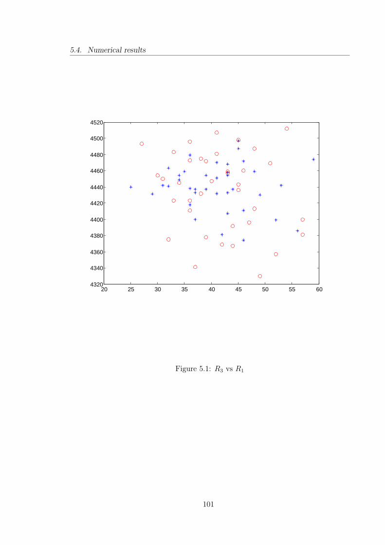
5.4. Numerical results
20 25 30 35 40 45 50 55 604320
4340
4360
4380
4400
4420
4440
4460
4480
4500
4520
Figure 5.1: R3 vs R1
101
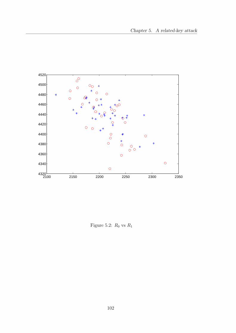
Chapter 5. A related-key attack
2100 2150 2200 2250 2300 23504320
4340
4360
4380
4400
4420
4440
4460
4480
4500
4520
Figure 5.2: R0 vs R1
102

5.4. Numerical results
2100 2150 2200 2250 2300 235020
25
30
35
40
45
50
55
60
Figure 5.3: R0 vs R3
103

Chapter 5. A related-key attack
940 960 980 1000 1020 1040 1060 1080 1100 1120 114020
25
30
35
40
45
50
55
60
Figure 5.4: R2 +R3 vs R3
104

5.5. Comments
This suggests that we would need to look at R1 in order to find some statisticalevidence. The expected R1-mean is 4436, the mean of dots is 4435 and the meanof stars is 4440. Although our mean is further from the expected mean than thedots mean (which is nearly the same as the expected), the difference is not statisticalsignificant and a Marsaglia-type test fails. However, it is not the mean that concernsus, but the fact that the stars are closer to their own mean. To point out the differencein statistical terms, we consider the number of stars within the expected standarddeviation range (4386 ≤ R1 ≤ 4486) and we compare it with the expected numberof values within the same range. The χ2 test gives in this case a probability of 0.5%
that the stars come from a random sample. This is a very strong confidence margin.To check the effectiveness of our test, we took four random samples and we appliedit. From the χ2 test we obtain probabilities of 63%, 64%, 28%, 24%, which do notshow any significant difference and are much higher than the probability obtained byour related-key sample. Therefore, our test is validated.
5.5 Comments
There are several comments and remarks that we feel are relevant for our attack:
• The matrix H that we constructed in the AES case is very closely correlated,since all rows come from just five original rows, with only three bytes varying; wedid try with less closely correlated matrices (for instance, with more free bytes,or with more starting rows), but we failed to note any significant deviation fromthe random behaviour.We also tried to increase further the correlation (by reducing the number of freebytes and/or the number of rows in D), but as a result we had a large number ofcollisions (i.e. of rows which were the same) and we could not make a workingmatrix.Therefore, our choice of |D| = 5 and 3 free bytes appear optimal, given ourpresent data.
• We tried to transform our related-key distinguishing attack into a single-keydistinguishing attack, but taking related matrices with a random key did notshow any statistical deviation.However, we tried a single-key version of our attack on reduced versions ofAES128 and it does show some statistical deviation for a few rounds. Since wewere not so interested in reduced versions of AES, we do not report here thereresults.
105

Chapter 5. A related-key attack
• We have mounted our attack also for the PRESENT cipher. Although the cipheris much smaller, the attack is not much simpler, because we cannot exploit thebyte-oriented structure held by AES. Our preliminary results are encouraging,but we do not report them here.
• Although algebraic setting for the attack is rather involved, the statistical testitself is very easy. We can design more sophisticated test, but we need more Skto apply them with significance.
106

Appendix
107


Appendix
Here we put the S-boxes of DES.
S1
14 4 13 1 2 15 11 8 3 10 6 12 5 9 0 70 15 7 4 14 2 13 1 10 6 12 11 9 5 3 84 1 14 8 13 6 2 11 15 12 9 7 3 10 5 015 12 8 2 4 9 1 7 5 11 3 14 10 0 6 13
S2
15 1 8 14 6 11 3 4 9 7 2 13 12 0 5 103 13 4 7 15 2 8 14 12 0 1 10 6 9 11 50 14 7 11 10 4 13 1 5 8 12 6 9 3 2 1513 8 10 1 3 15 4 2 11 7 6 12 0 5 14 9
S3
10 0 9 14 6 3 15 5 1 13 12 7 11 4 2 813 7 0 9 3 4 6 10 2 8 5 14 12 11 15 113 6 4 9 8 15 3 0 11 1 2 12 5 10 14 71 10 13 0 6 9 8 7 4 15 14 3 11 5 2 12
S4
7 13 14 3 0 6 9 10 1 2 8 5 11 12 4 1513 8 11 5 6 15 0 3 4 7 2 12 1 10 14 910 6 9 0 12 11 7 13 15 1 3 14 5 2 8 43 15 0 6 10 1 13 8 9 4 5 11 12 7 2 14
S5
2 12 4 1 7 10 11 6 8 5 3 15 13 0 14 914 11 2 12 4 7 13 1 5 0 15 10 3 9 8 64 2 1 11 10 13 7 8 15 9 12 5 6 3 0 1411 8 12 7 1 14 2 13 6 15 0 9 10 5 5 3
109

Chapter 6. Appendix
S6
12 1 10 15 9 2 6 8 0 13 3 4 14 7 5 1110 15 4 2 7 12 9 5 6 1 13 14 0 11 3 89 14 15 5 2 8 12 3 7 0 4 10 1 13 11 64 3 2 12 9 5 15 10 11 14 1 7 6 0 8 13
S7
4 11 2 14 15 0 8 13 3 12 9 7 5 10 6 113 0 11 7 4 9 1 10 14 3 5 12 2 15 8 61 4 11 13 12 3 7 14 10 15 6 8 0 5 9 26 11 13 8 1 4 10 7 9 5 0 15 14 2 3 12
S8
13 2 8 4 6 15 11 1 10 9 3 14 5 0 12 71 15 13 8 10 3 7 4 12 5 6 11 0 14 9 27 11 4 1 9 12 14 2 0 6 10 13 15 3 5 82 1 14 7 4 10 8 13 15 12 9 0 3 5 6 11
110

Bibliography
[ABKL+07] A. Andrey Bogdanov, L. R. Knudsen, G. Leander, C. Paar,A. Poschmann, M. J. B. Robshaw, Y. Seurin, and C. Vikkelsoe,PRESENT: An ultra-lightweight block cipher, Proc. of CHES 2007,LNCS, vol. 4727, Springer, 2007, pp. 450–466.
[AC08] M. Albrecht and C. Cid, Algebraic techniques in differential cryptanaly-sis, Crypto. ePrint Arch., Rep. 2008/177, 2008, http://eprint.iacr.org/.
[BAK98] E. Biham, R.J. Anderson, and L.R. Knudsen, Serpent: A new blockcipher proposal, Proc. of FSE 1998, LNCS, vol. 1372, Springer, 1998,pp. 222–238.
[BB02a] E. Barkan and E. Biham, The Book of Rijndaels, Tech. report, IACRePrint Report, 2002/158, 2002.
[BB02b] , In how many ways can you write Rijndael?, Proc. of ASI-ACRYPT 2002, LNCS, vol. 2501, 2002, pp. 160–175.
[BCD+98] C. Burwick, D. Coppersmith, E. D’Avignon, R. Gennaro, S. Halevi,C. Jutla, S. M. Matyas, L. O’Connor, M. Peyravian, D. Safford, andZunic N., MARS — A candidate cipher for AES, NIST AES Proposal,1998.
[BD07] M. Brickenstein and A. Dreyer, PolyBoRi: A framework for Gröbnerbasis computations with Boolean polynomials, Elec. Proc. of MEGA 2007,2007, http://www.ricam.oeaw.ac.at/mega2007/electronic/26.pdf.
[BDCBP03] A. Biryukov, C. De Canniere, A. Braeken, and B. Preneel, A toolbox forcryptanalysis: Linear and affine equivalence algorithms, Proc.of EURO-CRYPT 2003, LNCS, vol. 2656, 2003, pp. 33–50.
[BDK05] E. Biham, O. Dunkelman, and N. Keller, Related-key boomerang andrectangle attacks, Proc. of EUROCRYPT 2005, LNCS, vol. 3494, 2005,pp. 507–525.
111

Bibliography
[BK00] E. Biham and N. Keller, Cryptanalysis of reduced variants of Rijndael,Proc. of AES3, 2000.
[BK09] A. Biryukov and D. Khovratovich, Related-key Cryptanalysis ofthe Full AES-192 and AES-256, Tech. report, IACR, 2009,http://eprint.iacr.org/2009/317.
[BPW06a] J. Buchmann, A. Pyshkin, and R. P. Weinmann, Block ciphers sensi-tive to Gröbner basis attacks, Proc. of CT-RSA 2006, LNCS, vol. 3860,Springer, 2006, pp. 313–331.
[BPW06b] , A zero-dimensional Gröbner basis for AES-128, Proc. ofFSE 2006, LNCS, vol. 4047, Springer, 2006, pp. 78–88.
[BS93] E. Biham and A. Shamir, Differential cryptanalysis of DES-like cryp-tosystems, J. of Cryptology 4 (1993), 3–72.
[Buc65] Bruno Buchberger, Ein Algorithmus zum Auffinden der Basisele-mente des Restklassenringes nach einem nulldimensionalen Polyno-mideal, Ph.D. thesis, Innsbruck, 1965.
[Buc06] B. Buchberger, Bruno Buchberger’s PhD thesis 1965: An algorithm forfinding the basis elements of the residue class ring of a zero dimensionalpolynomial ideal, J. Symb. Comput. 41 (2006), no. 3-4, 475–511.
[Cam99] P. J. Cameron, Permutation groups, London Mathematical Society Stu-dent Texts, vol. 45, Cambridge University Press, Cambridge, 1999.
[Carar] C. Carlet, Boolean methods and models, ch. Boolean Functions for Cryp-tography and Error Correcting Codes, Cambridge University Press, toappear.
[CDVSar] A. Caranti, F. Dalla Volta, and M. Sala, On some block ciphers andimprimitive groups, AAECC (to appear), 10.
[CGC03] NESSIE D20 - NESSIE security report, 2003,http://citeseer.ist.psu.edu/568219.html.
[CKK+01] J.H. Cheon, M. Kim, K. Kim, J.Y. Lee, and S. Kang, Improved impossibledifferential cryptanalysis of Rijndael and Crypton, Proc. of ICISC 2001,LNCS, vol. 2288, 2001, pp. 39–49.
112
Bibliography
[CKPS00] N. Courtois, A. Klimov, J. Patarin, and A. Shamir, Efficient algo-rithms for solving overdefined systems of multivariate polynomial equa-tions, Proc. of EUROCRYPT 2000, LNCS, vol. 1807, Springer, 2000,pp. 392–407.
[CMR05] C. Cid, S. Murphy, and M. J. B. Robshaw, Small scale variants of theAES, Proc. of FSE 2005, LNCS, vol. 3557, Springer, 2005, pp. 145–162.
[CMR07] , Algebraic aspects of the Advanced Encryption Standard,Springer, 2007.
[CP02] N. Courtois and J. Pieprzyk, Cryptanalysis of block ciphers with overde-fined systems of equations, Proc. of ASIACRYPT 2002, LNCS, vol. 2501,Springer, 2002, pp. 267–287.
[CW09] C. Cid and R. P. Weinmann, Block ciphers: algebraic cryptanalysis andGröbner bases, Gröbner Bases, Coding, and Cryptography (M. Sala,T. Mora, L. Perret, S. Sakata, and C. Traverso, eds.), RISC Book Series,Springer, Heidelberg, 2009, p. to appear.
[CYK09] D. L. Cook, M. Yung, and A. D. Keromytis, Elastic block ciphers:method, security and instantiations, Int. J. Inf. Sec 8 (2009), no. 3, 211–231.
[Dar08] M. R. Darafsheh, The maximum element order in the groups related tothe linear groups which is a multiple of the defining characteristic, FiniteFields Appl. 14 (2008), no. 4, 992–1001.
[DKR97] J. Deamen, L. Knudsen, and V. Rijmen, The block cipher Square, Proc.of FSE 97, LNCS, vol. 1267, 1997, pp. 149–165.
[DM96] J. D. Dixon and B. Mortimer, Permutation groups, vol. 163, Springer-Verlag, 1996.
[DR98] J. Daemen and V. Rijmen, AES proposal: Rijndael, Tech. report, NIST,1998.
[DR02] , The Design of Rijndael, Springer, 2002.
[FKL+00] N. Ferguson, J. Kesley, S. Lucks, B. Schneier, M. Stay, D. Wagner,and D. Whitinf, Improved cryptanalysis of Rijndael, Proc. of FSE 2000,LNCS, vol. 1978, Springer, 2000, pp. 213–230.
113

Bibliography
[FSW01] N. Ferguson, R. Schroeppel, and D. Whitinf, A simple algebraic represen-tation of Rijndael, Proc. of SAC 2001, LNCS, vol. 2259, 2001, pp. 103–111.
[GM00] H. Gilbert and M. Minier, A collision attack on seven rounds of Rijndael,Proc. of AES3, 2000.
[KKS00] J. Kelsey, T. Kohno, and B. Schneier, Amplified Boomerang attackagainst reduced-round MARS and Serpent, Proc. of FSE 2000, LNCS,vol. 1978, 2000, pp. 75–93.
[KL90] P. Kleidman and M. Liebeck, The subgroup structure of the finite classicalgroups, London Math. Soc. LNS, vol. 129, Cambridge University Press,1990.
[Knu99] L. Knudsen, Contemporary block ciphers, LNCS 1561 (1999), 105–126.
[Lan03] E. Landau, Ueber die maximalordung der permutation gegbenen grades,Arch. der Math. und Phys. 5 (1903), no. 3, 92–103.
[LK07] C. Lim and K. Khoo, An Analysis of XSL applied to BES, Proc. ofFSE 2007 (A. Biryukov, ed.), LNCS, vol. 4593, Springer, 2007, pp. 242–253.
[LN97] R. Lidl and H. Niederreiter, Finite fields, Encyclopedia of Mathematicsand its Applications, Cambridge University Press, 1997.
[Mai09] Lara Maines, Una debole rappresentazione del gruppo simmetrico, Mas-ter’s thesis (laurea specialistica), University of Trento, Department ofMathematics, 2009.
[Mat93] M. Matsui, Linear cryptanalysis method for DES cipher, Proc. of EU-ROCRYPT 93, LNCS, vol. 765, 1993, pp. 386–397.
[MMM04] T. Migler, K. E. Morrison, and O. Mitchell, Weight andrank of matrices over finite fields, Tech. report, arxiv, 2004,http://arxiv.org/abs/math/0403314.
[MR02] S. Murphy and M. J. B. Robshaw, Essential algebraic structure within theAES, Proc. of CRYPTO 2002, LNCS, vol. 2442, Springer, 2002, pp. 1–16.
[Nat77] National Bureau of Standards, The Data Encryption Standard, FederalInformation Processing Standards Publication (FIPS) 46, 1977.
114

Bibliography
[Nat01] National Institute of Standards and Technology, The Advanced Encryp-tion Standard, Federal Information Processing Standards Publication(FIPS) 197, 2001.
[NIS00] A statistical test suite for random and pseudorandom number gener-ators for cryptographic applications, Special Publication SP 800-22,NIST, 2000, http://csrc.nist.gov/publications/nistpubs/800-22/sp-800-22-051501.pdf.
[PGC98] J. Patarin, L. Goubin, and N. Courtois, Improved algorithms for isomor-phisms of polynomials, Proc. of EUROCRYPT 1998, LNCS, vol. 1403,1998, pp. 184–200.
[Pha04] R. C. W. Phan, Impossible differential cryptanalysis of 7-round advancedencryption standard (AES), Inform. Process. Lett. 91 (2004), no. 1, 33–38.
[pol] The software package PolyBori - Polynomials over Boolean Rings,http://polybori.sourceforge.net/.
[Riv92] R. L. Rivest, The MD5 message-digest algorithm, Internet RFC 1321,1992.
[RRY00] R. L. Rivest, M. J. B. Robshaw, and Y. L. Yin, RC6 as the AES, Proc.of AES III, 2000, pp. 337–342.
[Rue92] R. Rueppel, Stream ciphers, Contemporary cryptology - The science ofinformation integrity, IEEE Press, 1992, pp. 65–134.
[Sch98] B. Schneier, The Twofish encryption algorithm, Dr. Dobb’s Journal ofSoftware Tools 23 (1998), no. 12, 30–38.
[Sha49] C. E. Shannon, Communication theory of secrecy systems, Bell SystemTech. J. 28 (1949), 656–715.
[Sot98] J. J. Soto, Randomness testing of the AES candidate algo-rithms, Proc. of AES candidate conference I (National In-stitute of Standards and Technology, ed.), NIST, 1998,http://csrc.nist.gov/encryption/aes/round1/r1-rand.pdf, p. 9.
[Sti95] D. R. Stinson, Cryptography, Theory and Practice, CRC Press, 1995.
[SW08] R. Sparr and R. Wernsdorf, Group theoretic properties of Rijndael-likeciphers, Discrete Appl. Math. 156 (2008), no. 16, 3139–3149.
115

Bibliography
[TZ05] I. Toli and A. Zanoni, An algebraic interpretation of AES-128, Proc. ofAES 2004, LNCS, vol. 3373, Springer, 2005, pp. 84–97.
[Wag76] A. Wagner, The faithful linear representation of least degree of sn andan over field of characteristic 2., Math. Z. 151 (1976), no. 2, 127–137.
[Wag99] D. Wagner, The Boomerang attack, Proc. of FSE 1999, LNCS, vol. 1636,1999, pp. 156–170.
[Wer02] R. Wernsdorf, The round functions of Rijndael generate the alternatinggroup, Proc. of FSE 2002, LNCS, vol. 2365, Springer, 2002, pp. 143–148.
[WLL04] S. Wu, S. Lu, and C. Laih, Design of AES based on dual cipher andcomposite field, Proc. of CT-RSA 2004, LNCS, vol. 2964, 2004, pp. 25–38.
[WOL02] J. Wolkerstorfer, E. Oswald, and M. Lamberger, An ASIC implementa-tion of the AES SBoxes, CT-RSA: The Cryptographers’ Track at RSAConference, LNCS, vol. 2271, 2002, pp. 67–68.
116