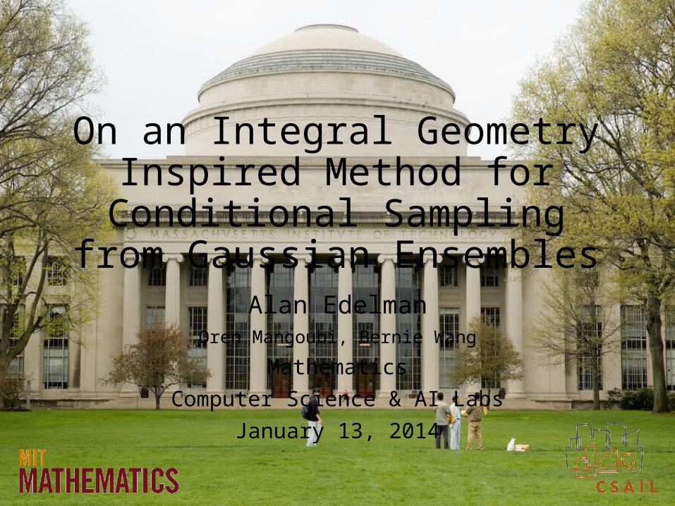
On an Integral Geometry Inspired Method for

Conditional Sampling from Gaussian Ensembles

Alan EdelmanOren Mangoubi, Bernie Wang

MathematicsComputer Science & AI Labs

January 13, 2014

Talk Sandwich

• Stories ``Lost and Found”: Random Matrices in the years 1955-1965

• Integral Geometry Inspired Method for Conditional Sampling from Gaussian Ensembles

• Demo: On the higher order correction of the distribution of the smallest singular value

Stories “Lost and Found”

Random Matrices in the Years 1955-1965

Lost and Found

• Wigner thanks Narayana• Ironically, Narayana (1930-1987) probably never knew

that his polynomials are the moments for Laguerre (Catalan:Hermite :: Narayana:Laguerre)

• The statistics/physics links were severed• Wigner knew Wishart matrices• Even dubbed the GOE ``the Wishart set’’

• Numerical Simulation was common (starting 1958)• Art of simulation seems lost for many decades and then

refound

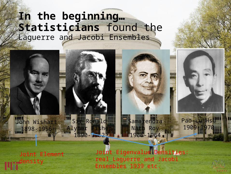
In the beginning…Statisticians found theLaguerre and Jacobi Ensembles

John Wishart1898-1956

Sir Ronald Alymer Fisher1890-1962

Samarendra Nath Roy

1906-1964

Pao-Lu Hsu1909-1970

Joint Eigenvalue Densities: real Laguerre and Jacobi Ensembles 1939 etc.

Joint Element density

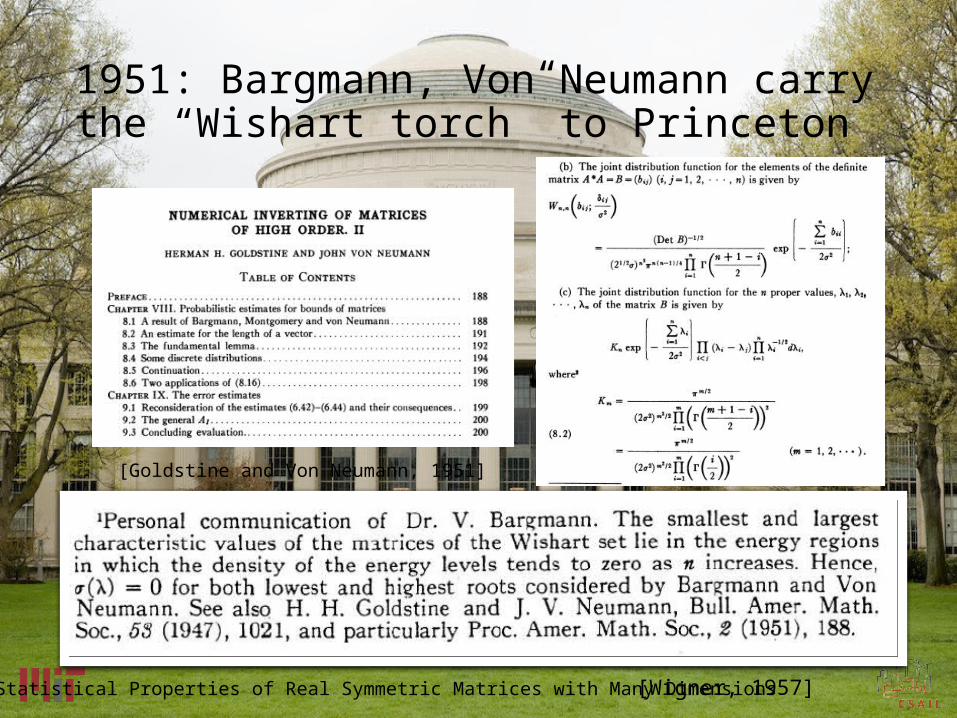
1951: Bargmann, Von Neumann carry the “Wishart torch” to Princeton

[Wigner, 1957]

[Goldstine and Von Neumann, 1951]

Statistical Properties of Real Symmetric Matrices with Many Dimensions

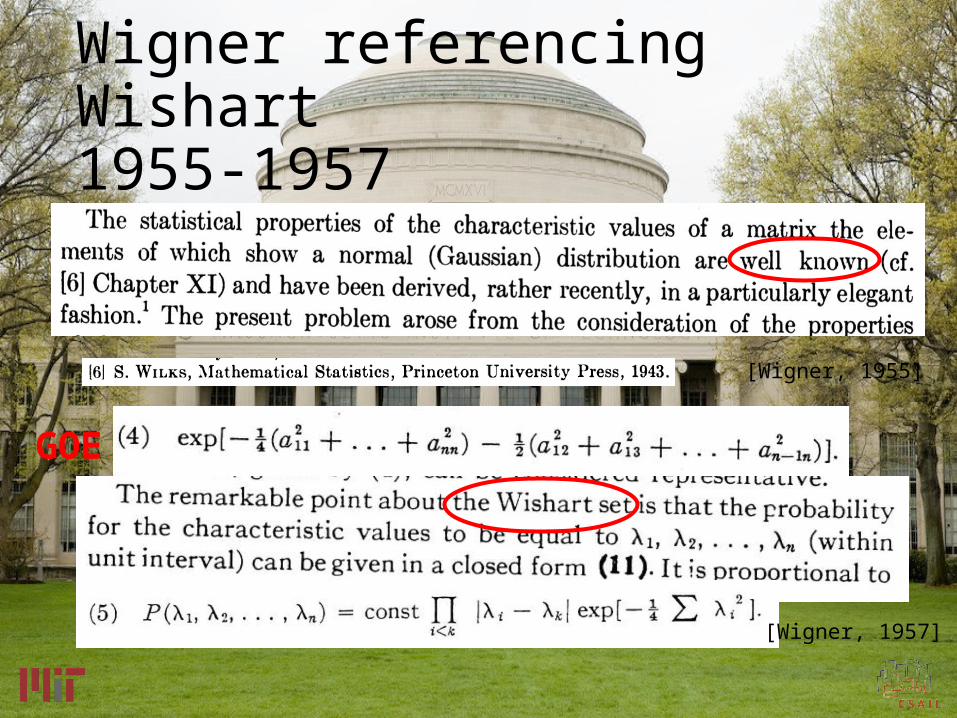
Wigner referencing Wishart1955-1957

GOE

[Wigner, 1955]

[Wigner, 1957]

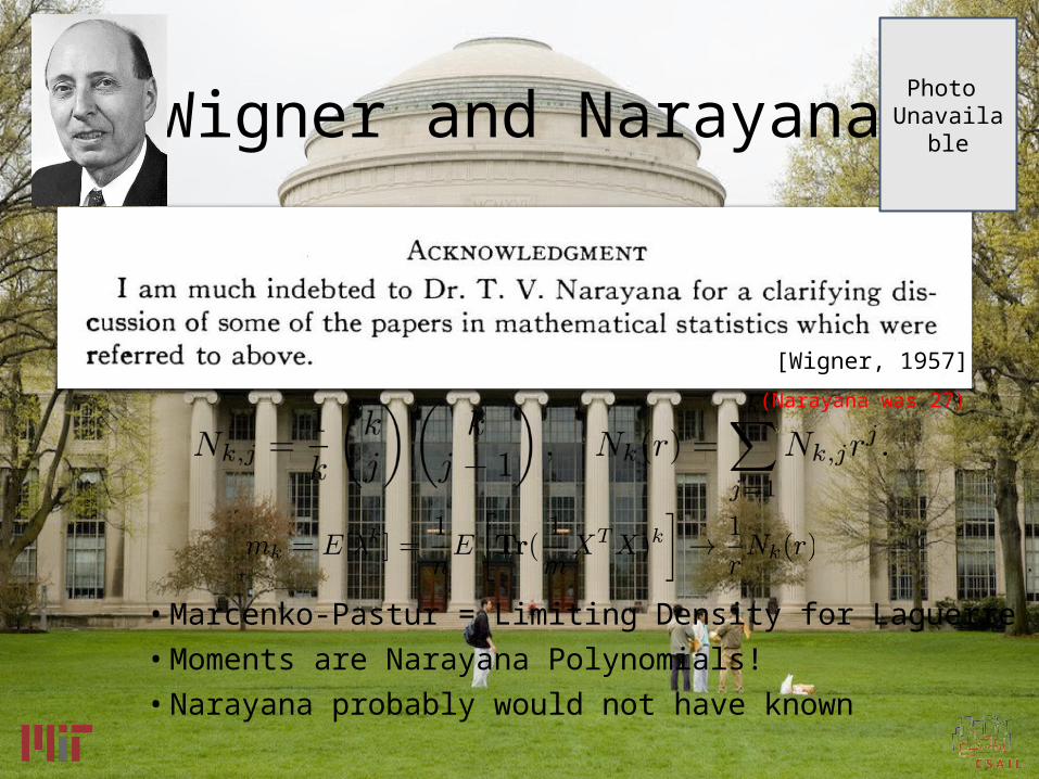
Wigner and Narayana

• Marcenko-Pastur = Limiting Density for Laguerre• Moments are Narayana Polynomials!• Narayana probably would not have known

[Wigner, 1957]

Photo Unavailable

(Narayana was 27)

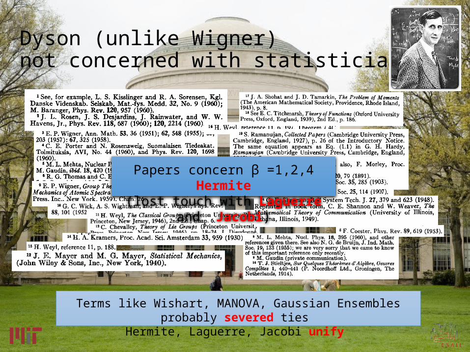
Dyson (unlike Wigner) not concerned with statisticians

Terms like Wishart, MANOVA, Gaussian Ensembles probably severed ties Hermite, Laguerre, Jacobi unify

Papers concern β =1,2,4 Hermite(lost touch with Laguerre and Jacobi)

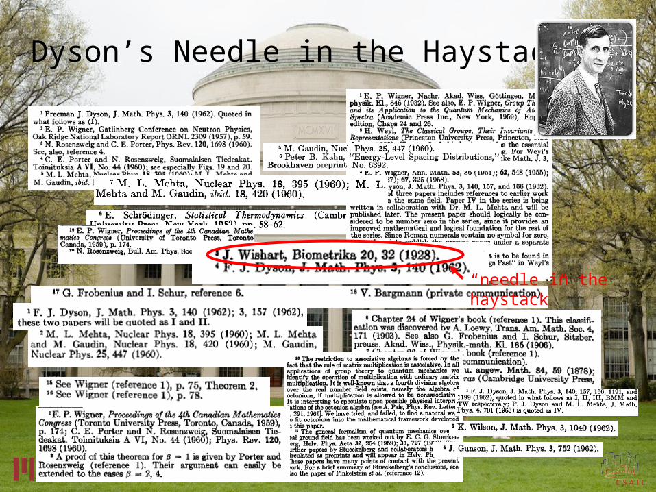
Dyson’s Needle in the Haystack

“needle in the haystack”

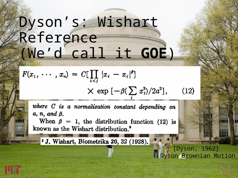
Dyson’s: Wishart Reference(We’d call it GOE)

[Dyson, 1962] Dyson Brownian Motion

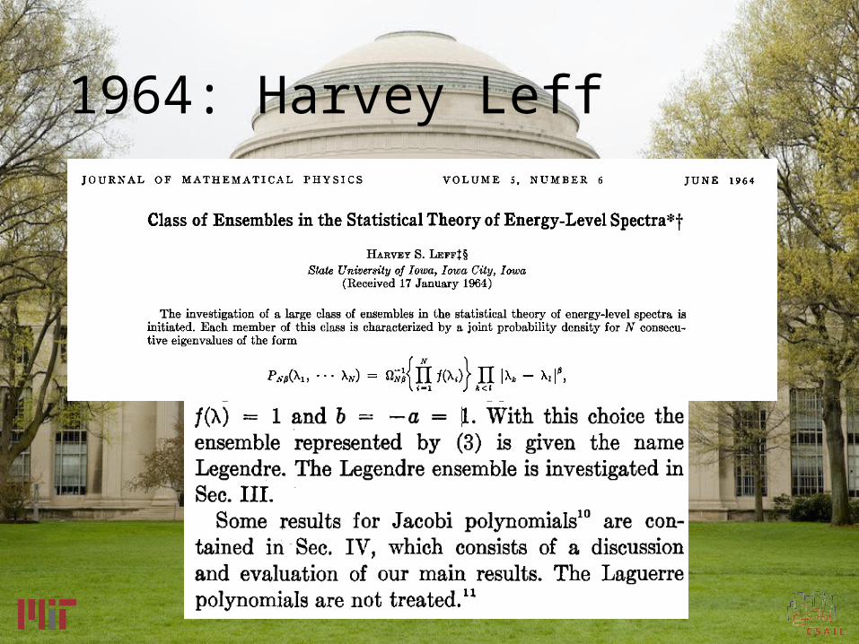
1964: Harvey Leff

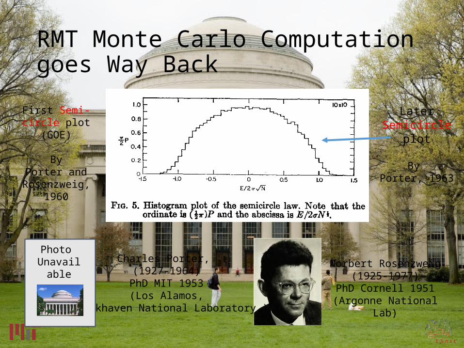
RMT Monte Carlo Computationgoes Way Back

Norbert Rosenzweig(1925-1977)

PhD Cornell 1951(Argonne National Lab)

Charles Porter, (1927-1964)

PhD MIT 1953(Los Alamos,

Brookhaven National Laboratory )

Photo Unavailable

First Semi-circle plot (GOE)

ByPorter and

Rosenzweig, 1960

Later Semicircle plot

By Porter, 1963

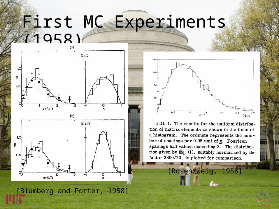
First MC Experiments (1958)

[Blumberg and Porter, 1958]

[Rosenzweig, 1958]

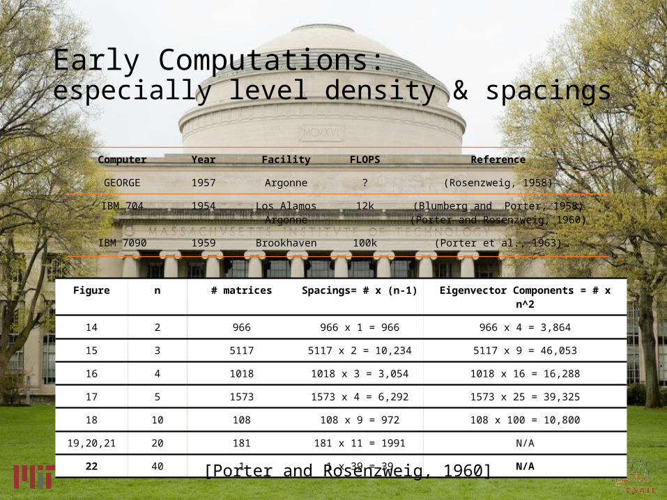
Early Computations:especially level density & spacings

Computer Year Facility FLOPS Reference

GEORGE 1957 Argonne ? (Rosenzweig, 1958)

IBM 704 1954 Los AlamosArgonne

12k (Blumberg and Porter, 1958)(Porter and Rosenzweig, 1960)

IBM 7090 1959 Brookhaven 100k (Porter et al., 1963)

Figure n # matrices Spacings= # x (n-1) Eigenvector Components = # x n^2

14 2 966 966 x 1 = 966 966 x 4 = 3,864

15 3 5117 5117 x 2 = 10,234 5117 x 9 = 46,053

16 4 1018 1018 x 3 = 3,054 1018 x 16 = 16,288

17 5 1573 1573 x 4 = 6,292 1573 x 25 = 39,325

18 10 108 108 x 9 = 972 108 x 100 = 10,800

19,20,21 20 181 181 x 11 = 1991 N/A

22 40 1 1 x 39 = 39 N/A

[Porter and Rosenzweig, 1960]

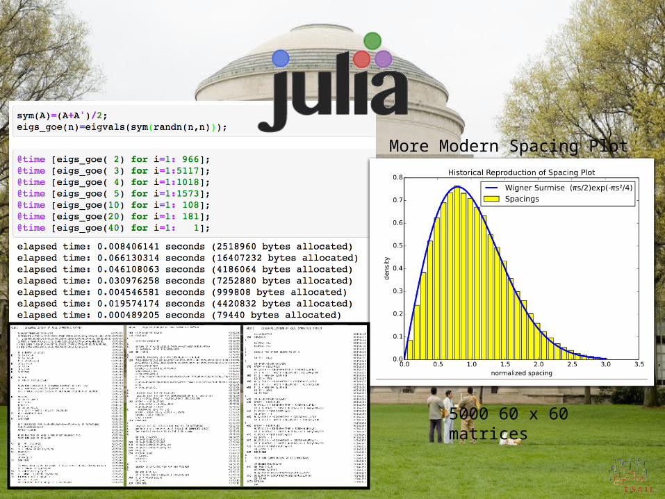
5000 60 x 60 matrices

More Modern Spacing Plot

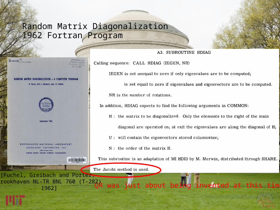
Random Matrix Diagonalization1962 Fortran Program

QR was just about being invented at this time

[Fuchel, Greibach and Porter, Brookhaven NL-TR BNL 760 (T-282)

1962]

On an Integral Geometry Inspired Method for

Conditional Sampling from Gaussian Ensembles

Outline

• Motivation: General β Tracy-Widom• Crofton’s Formula• The Algorithm for

• Conditional Probability• Special Case: Density Estimation

• Code• Application: General β Tracy-Widom

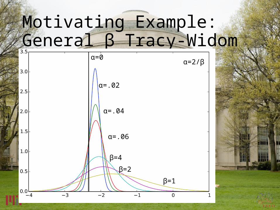
Motivating Example: General β Tracy-Widom

α=2/β

α=.02

α=.04

α=.06

β=4

β=2

β=1

α=0

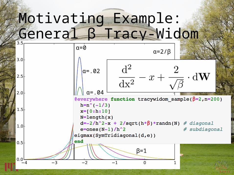
Motivating Example: General β Tracy-Widom

α=2/β

α=.02

α=.04

α=.6

β=4

β=2

β=1

α=0

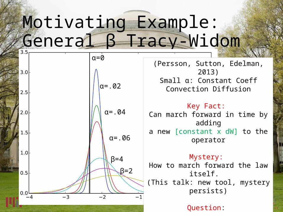
Motivating Example: General β Tracy-Widom

α=2/β

α=.02

α=.04

α=.06

β=4

β=2

β=1

α=0(Persson, Sutton, Edelman, 2013)

Small α: Constant Coeff Convection Diffusion

Key Fact: Can march forward in time by adding

a new [constant x dW] to the operator

Mystery: How to march forward the law itself. (This talk: new tool, mystery persists)

Question: Conditioned on starting at a point, how do

we diffuse?

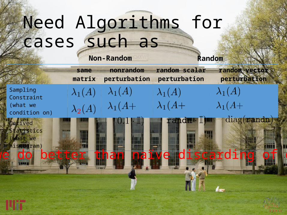
Need Algorithms for cases such as

same matrix

nonrandom perturbation

random scalar perturbation

random vector perturbation

Sampling Constraint(what we condition on)

Derived Statistics (what we histogram)

Can we do better than naïve discarding of data?

Random Non-Random

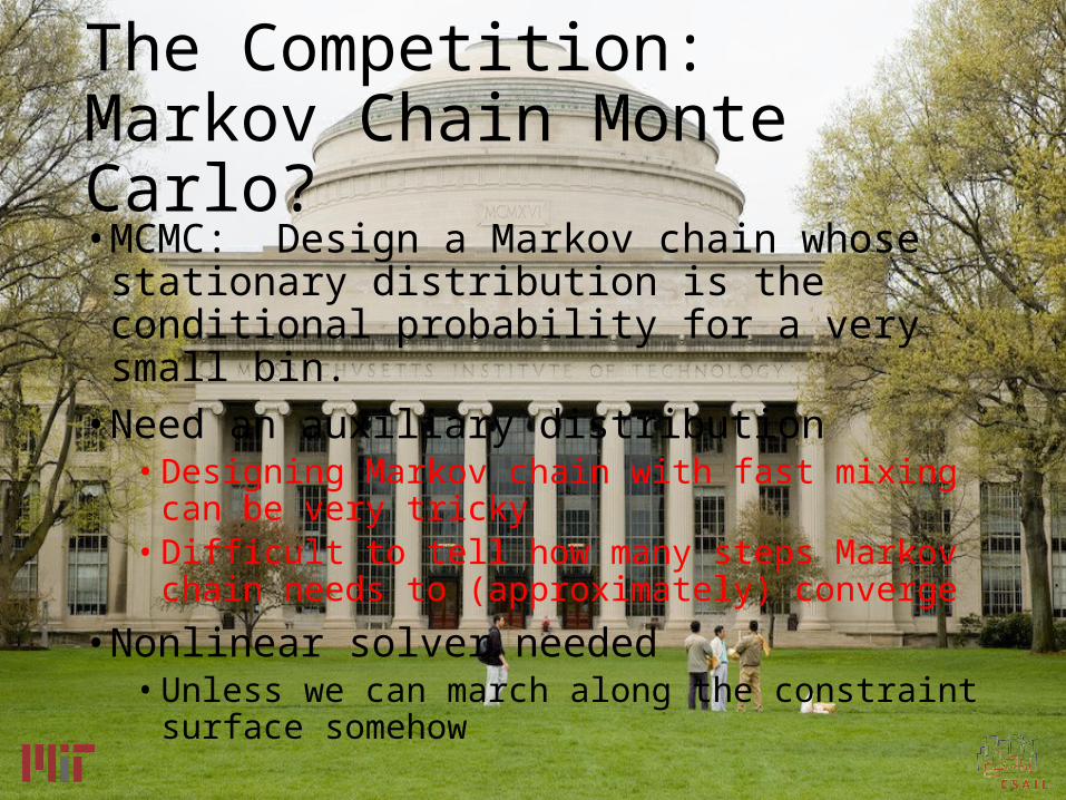
The Competition:Markov Chain Monte Carlo?• MCMC: Design a Markov chain whose stationary

distribution is the conditional probability for a very small bin.

• Need an auxiliary distribution• Designing Markov chain with fast mixing can be very tricky• Difficult to tell how many steps Markov chain needs to

(approximately) converge

• Nonlinear solver needed• Unless we can march along the constraint surface

somehow

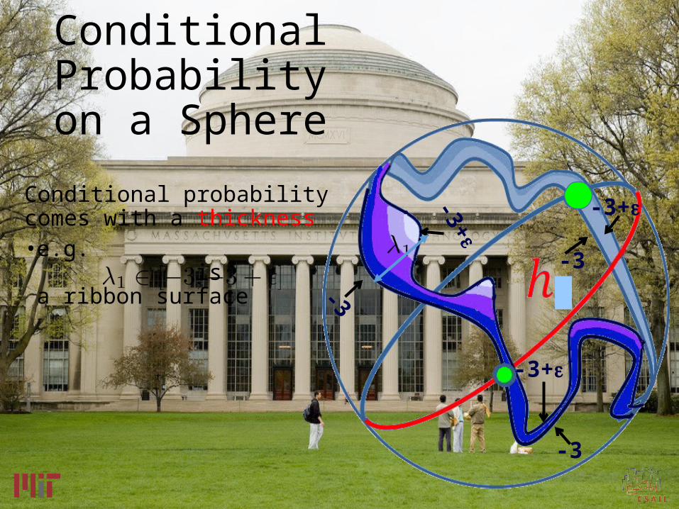
Conditional Probability on a Sphere

Conditional probability comes with a thickness• e.g. is

a ribbon surface -3

-3+

-3+

-3

-3+

-3

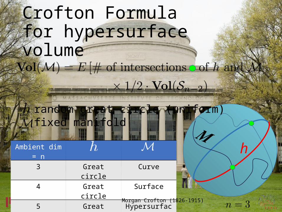
Crofton Formula for hypersurface volume

h𝑴

random great circle (uniform) fixed manifold

Ambient dim = n

3 Great circle Curve

4 Great circle Surface

5 Great circle Hypersurface

Morgan Crofton (1826-1915)

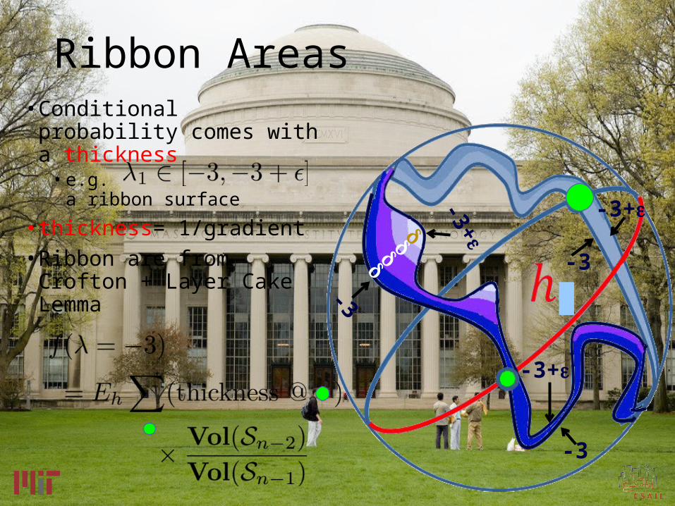
Ribbon Areas• Conditional probability

comes with a thickness• e.g.

a ribbon surface

• thickness= 1/gradient• Ribbon are from Crofton +

Layer Cake Lemma -3

-3+

-3+

-3

-3+

-3

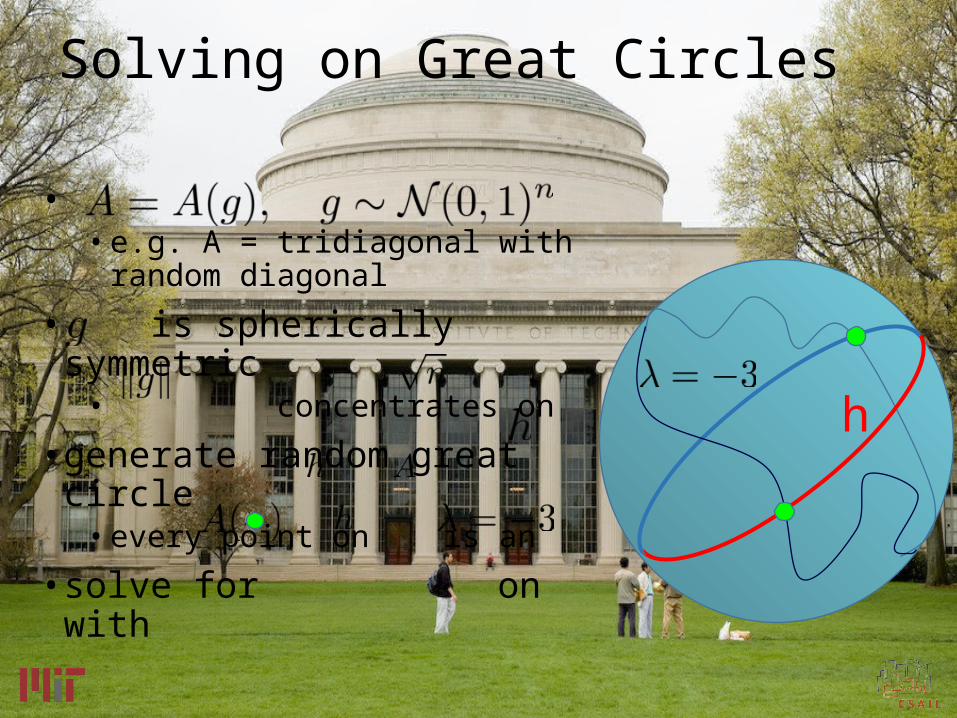
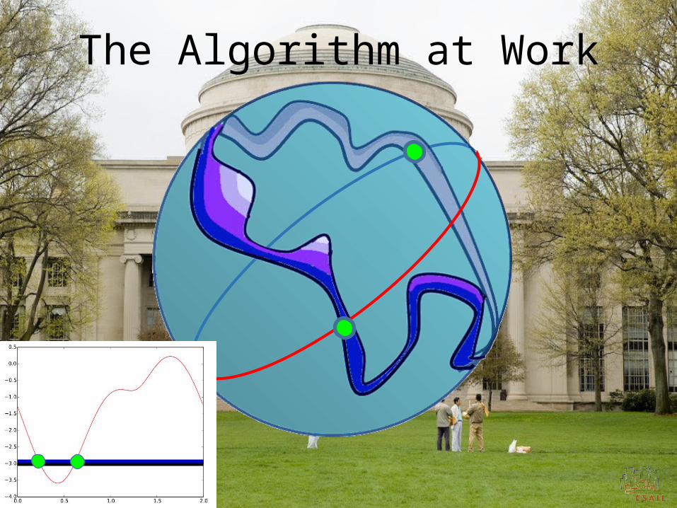
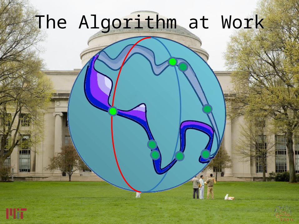
Solving on Great Circles

• • e.g. A = tridiagonal with random

diagonal

• is spherically symmetric• concentrates on

• generate random great circle • every point on is an

• solve for on with

h

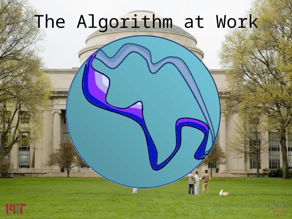
The Algorithm at Work

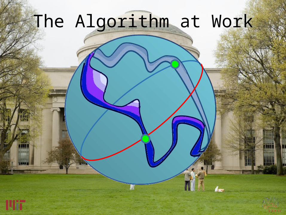
The Algorithm at Work

The Algorithm at Work

The Algorithm at Work

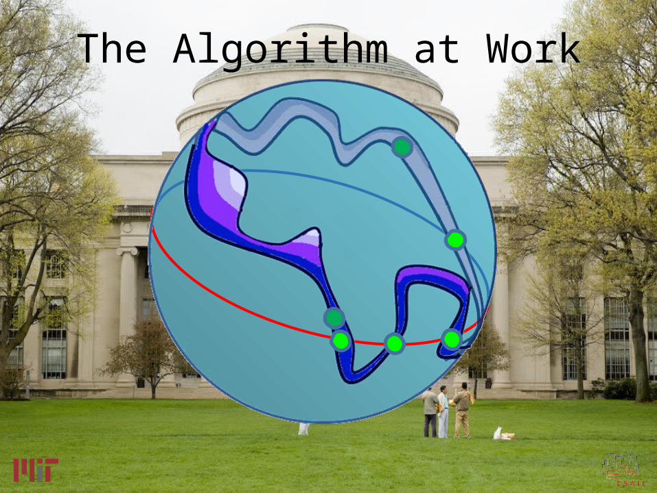
The Algorithm at Work

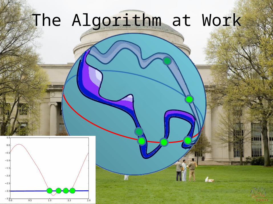
The Algorithm at Work

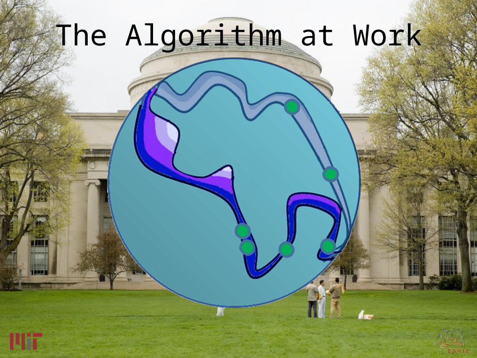
The Algorithm at Work

The Algorithm at Work

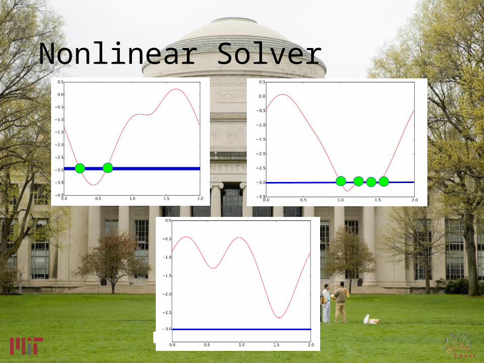
Nonlinear Solver

\\

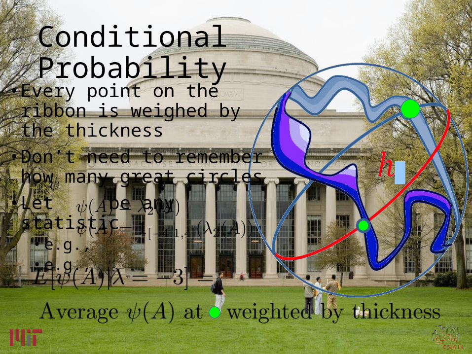
• Every point on the ribbon is weighed by the thickness

• Don’t need to remember how many great circles

• Let be any statistic• e.g., • e.g.,

Conditional Probability

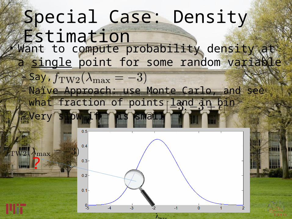
• Want to compute probability density at a single point for some random variable– Say, – Naïve Approach: use Monte Carlo, and see what

fraction of points land in bin – Very slow if is small

max

?

Special Case: Density Estimation

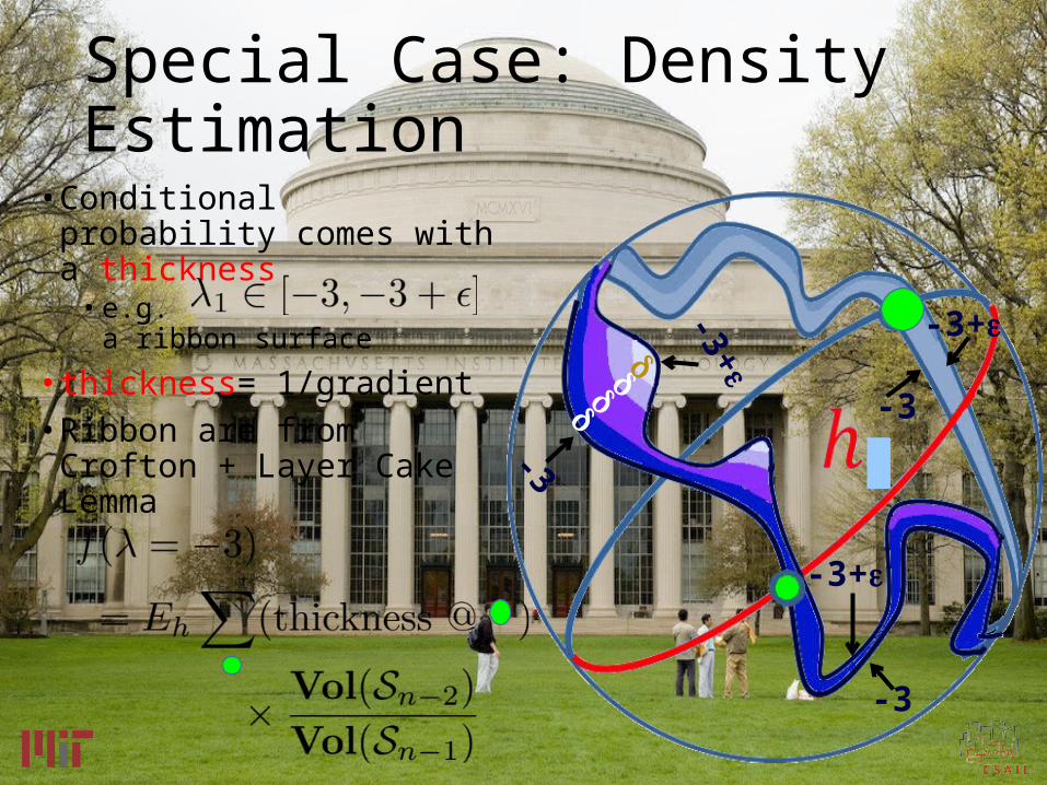
• Conditional probability comes with a thickness

• e.g. a ribbon surface

• thickness= 1/gradient• Ribbon are from Crofton +

Layer Cake Lemma-3

-3+

-3+

-3

-3+

-3

Special Case: Density Estimation

A good computational trick is also a good theoretical trick….

Integral Geometry and Crofton’s Formula• Rich History in Random Polynomial/Complexity

Theory/Bezout Theory• Kostlan, Shub, Smale, Rojas, Malajovich, more recent

works…

• We used it in: How many roots of a random real-coefficient polynomial are real?

• Should find a better place in random matrix theory

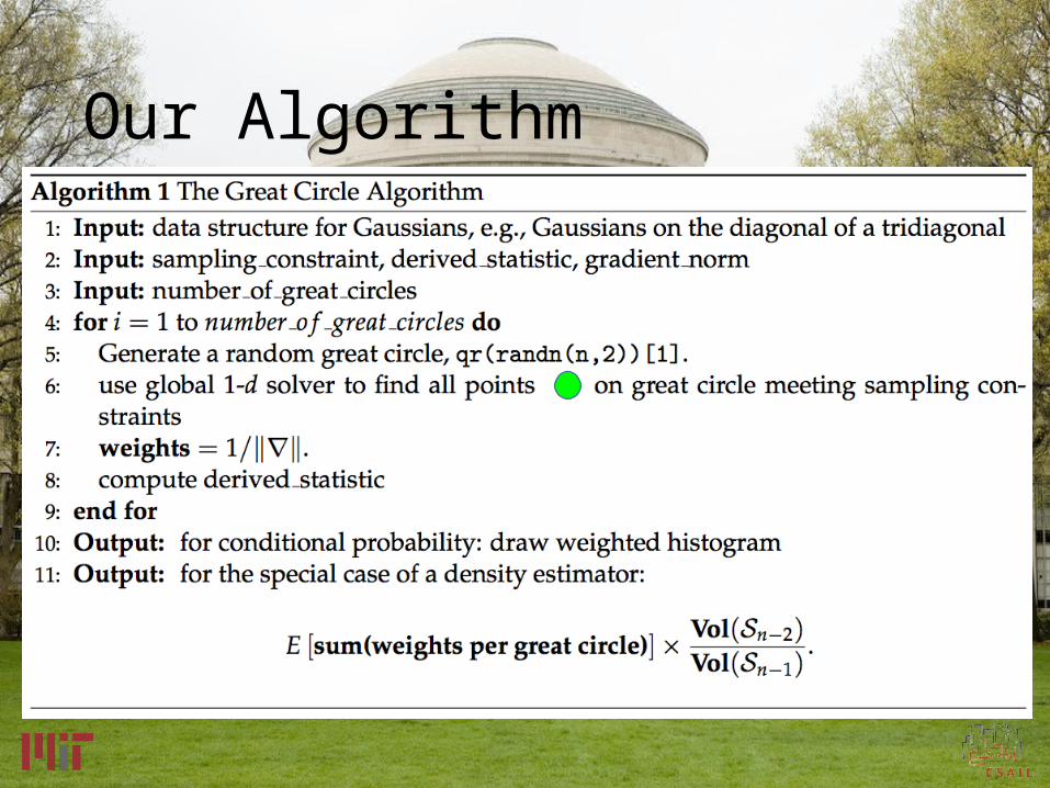
Our Algorithm

Step 4: parameters

Step 1: sampling constraint

Step 3: ||gradient(sampling constraint)||e.g.,

Step 2: derived statistic

Step 5: run the algorithm

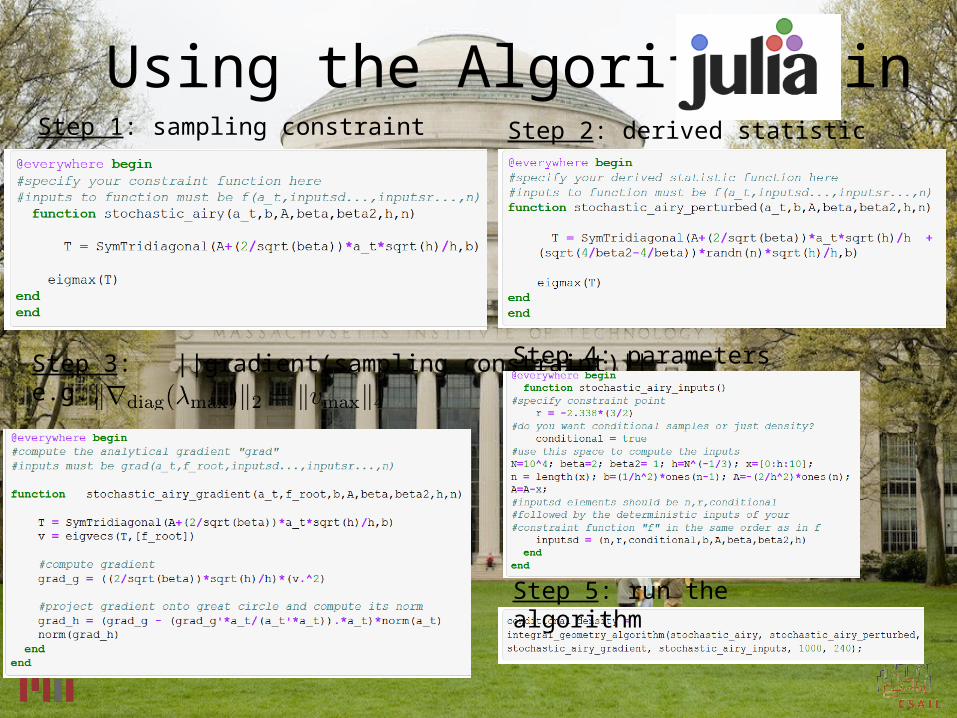
Using the Algorithm, in

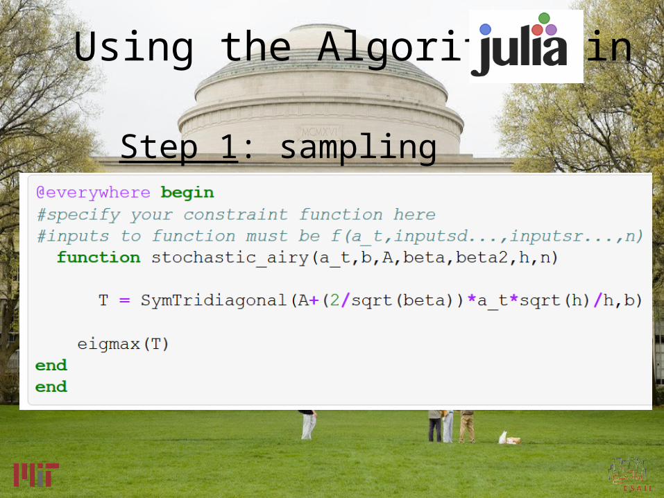
Step 1: sampling constraint

Using the Algorithm, in

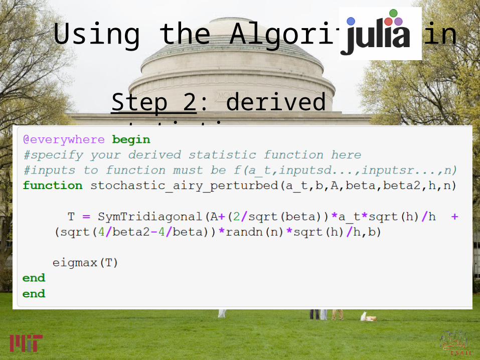
Step 2: derived statistic

Using the Algorithm, in

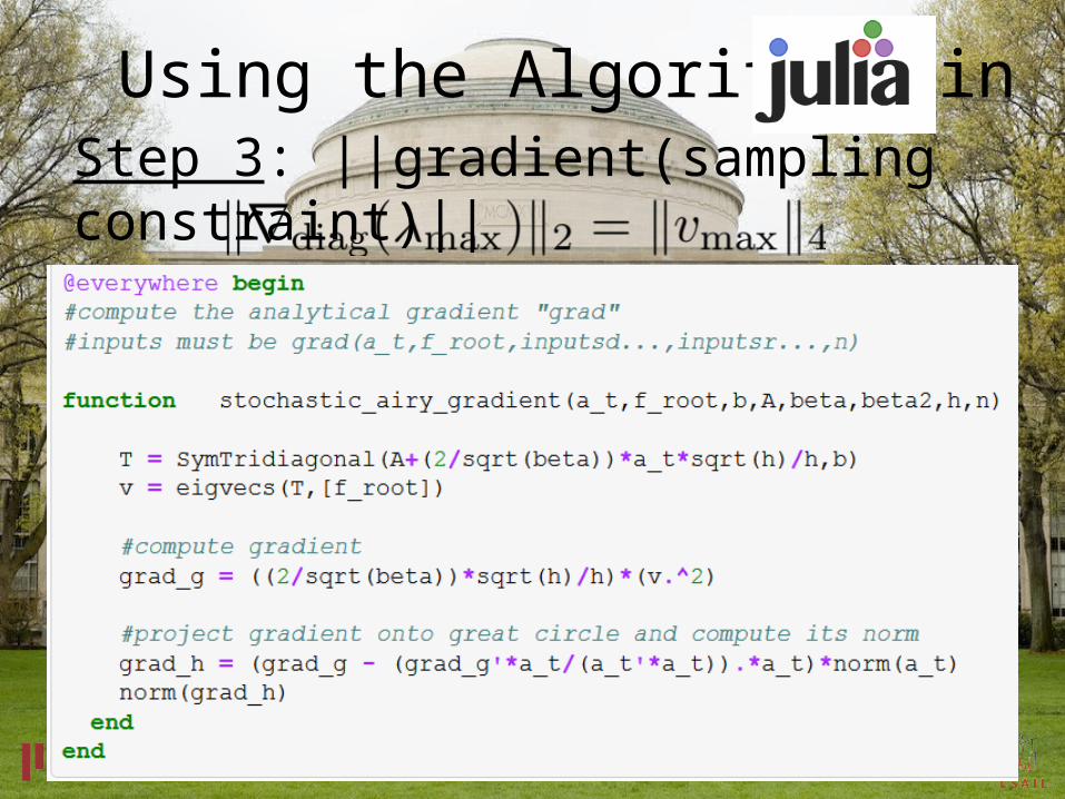
Step 3: ||gradient(sampling constraint)||e.g.,

Using the Algorithm, in

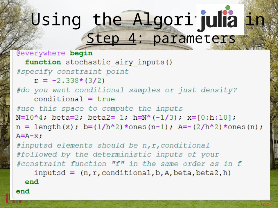
Step 4: parametersUsing the Algorithm, in

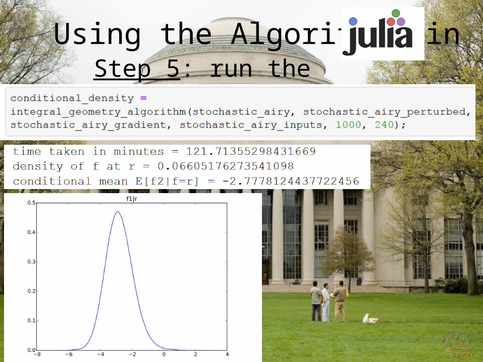
Step 5: run the algorithmUsing the Algorithm, in

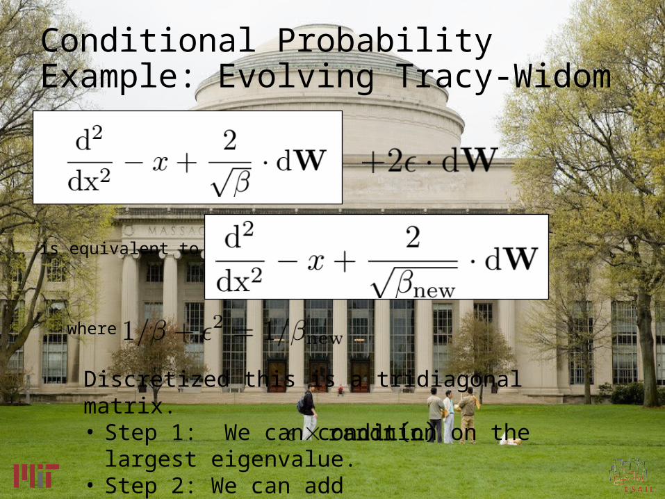
Conditional Probability Example: Evolving Tracy-Widom

is equivalent to

where

Discretized this is a tridiagonal matrix. • Step 1: We can condition on the largest eigenvalue.• Step 2: We can add to the diagonal

and histogram the new eigenvalue

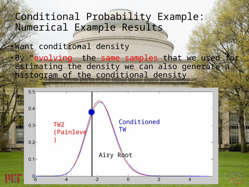
• Want conditional density• By “evolving” the same samples that we used for

estimating the density we can also generate a histogram of the conditional density

TW2 (Painleve)

Conditioned TW

Airy Root

Conditional Probability Example: Numerical Example Results

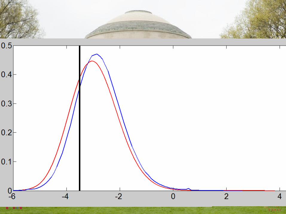
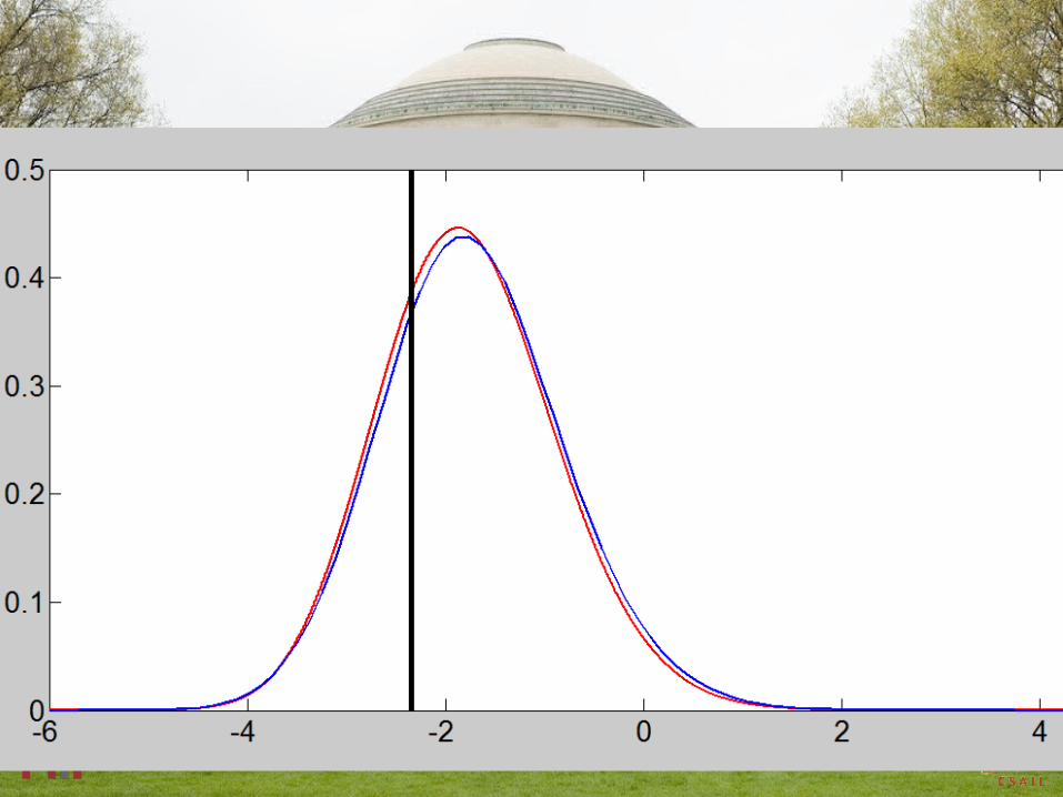
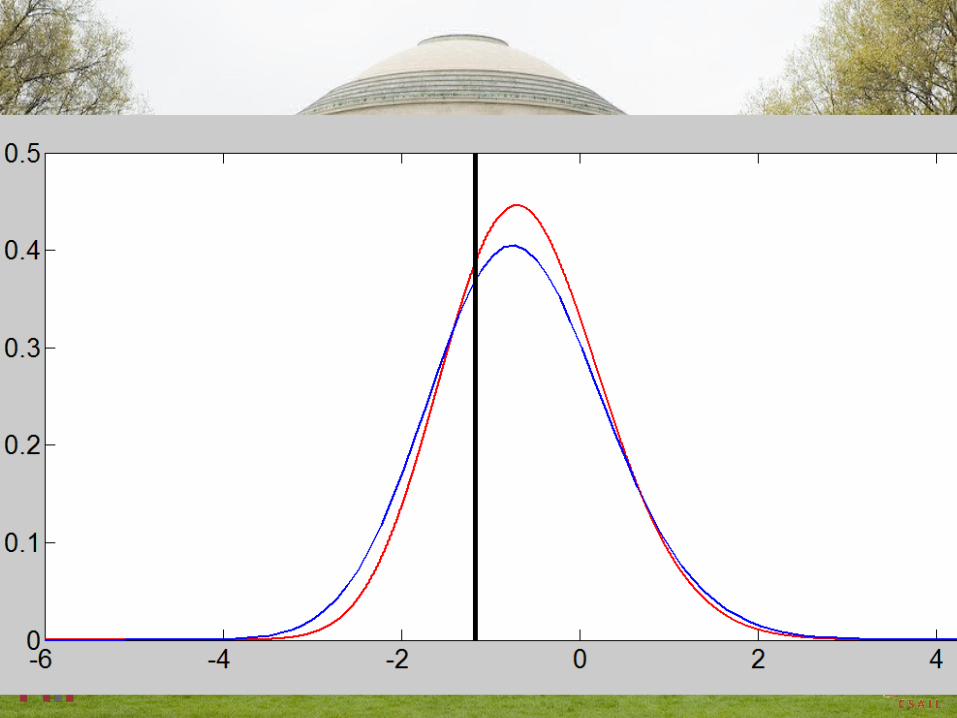
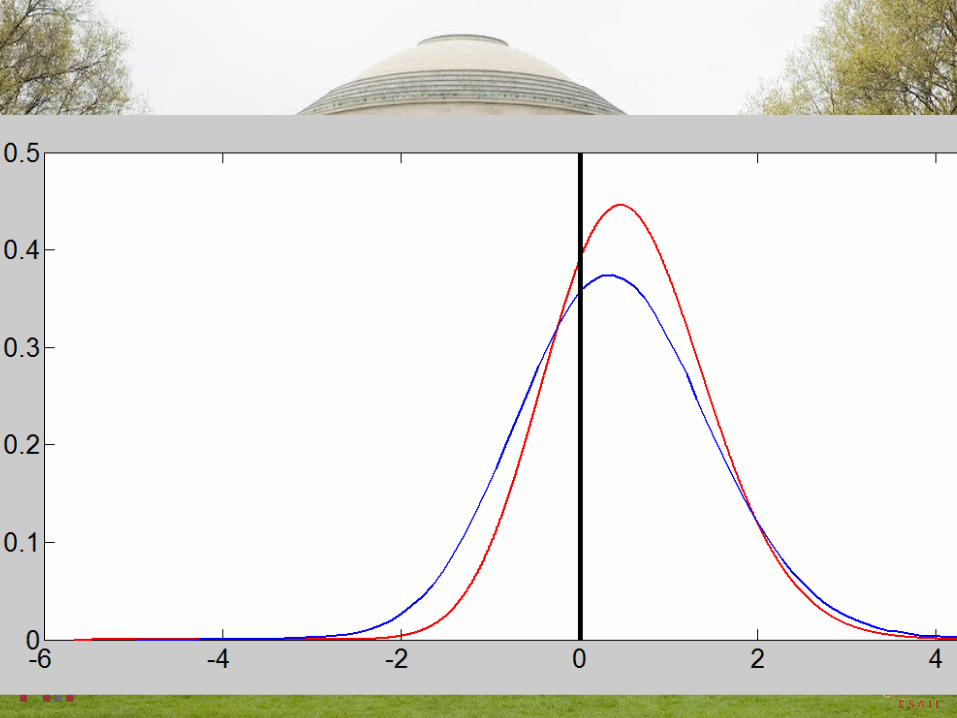
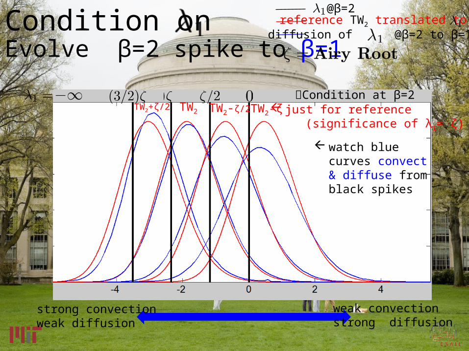
Condition on Evolve  β=2 spike to β=1

strong convectionweak diffusion

weak convectionstrong diffusion

reference TW2 translated to diffusion of @β=2 to β=1

@β=2

TW2 TW2-ζ/2 TW2-ζTW2+ζ/2 just for reference (significance of λ1= ζ)

watch blue curves convect & diffuse from black spikes

Condition at β=2

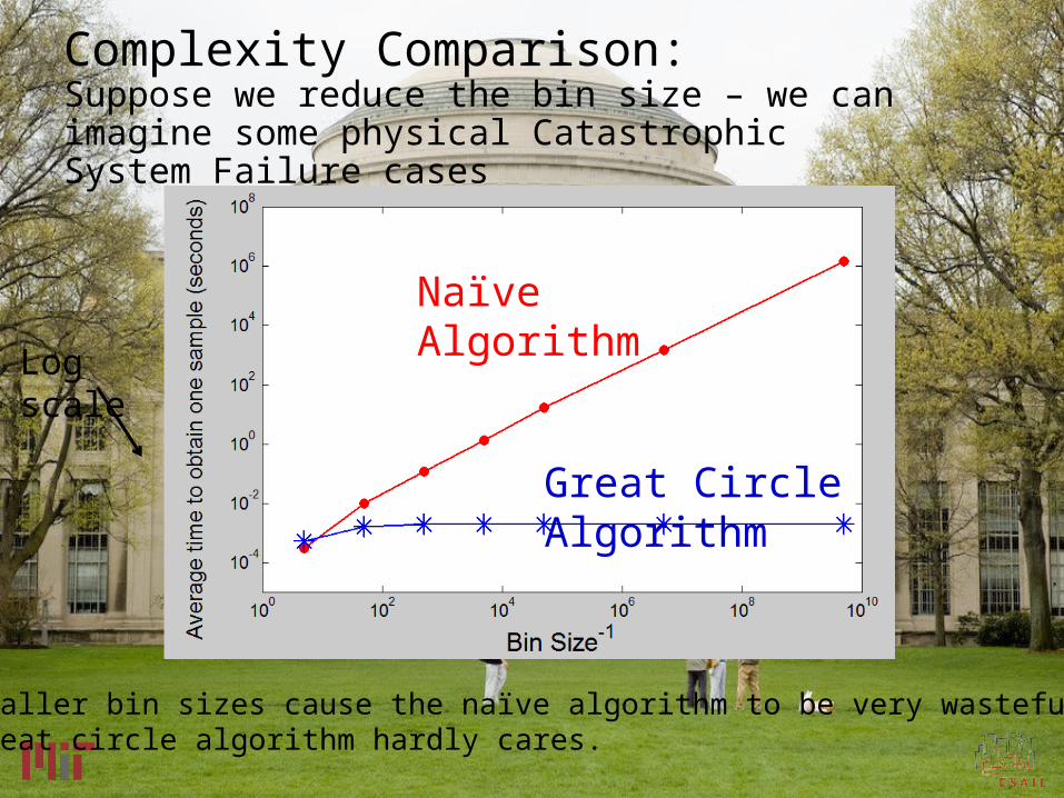
Complexity Comparison: Suppose we reduce the bin size – we can imagine some physical Catastrophic System Failure cases

Naïve Algorithm

Great Circle Algorithm

Log scale

Smaller bin sizes cause the naïve algorithm to be very wasteful. Great circle algorithm hardly cares.

• Higher Dimensional versions of Crofton’s formula

• Intersections of higher dimensional spheres with lower dimensional manifolds

Possible Extension:Conditioning on large numbers of variables

Applications• MLE for covariance matrix rank estimation

• Most covariance matrix models do not have analytical solution for eigenvalue densities

• Heavy tailed random matrices• Molecular interaction simulations (conditioning on

the rare phase change)• Stochastic PDE (also functions of )

• Weather simulation (conditioning on today’s incomplete weather, what is the probability of rain tomorrow?)

• Probability of airplane crashing (rare event)

• Deriving theoretical bounds for conditional probability ?? Other theory??

Acknowledgements• NDSEG Fellowship• Air Force Office of Scientific Research• NSF DMS 1035400 and DMS 1016125