Real-Time Syst (2008) 40: 208–237DOI 10.1007/s11241-008-9055-4

On earliest deadline first scheduling for temporalconsistency maintenance

Ming Xiong · Qiong Wang · Krithi Ramamritham

Published online: 5 June 2008© Springer Science+Business Media, LLC 2008

Abstract A real-time object is one whose state may become invalid with the passageof time. A temporal validity interval is associated with the object state, and the real-time object is temporally consistent if its temporal validity interval has not expired.Clearly, the problem of maintaining temporal consistency of data is motivated by theneed for a real-time system to track its environment correctly. Hence, sensor trans-actions must be able to execute periodically and also each instance of a transactionshould perform the relevant data update before its deadline.

Unfortunately, the period and deadline assignment problem for periodic sensortransactions has not received the attention that it deserves. An exception is the More-Less scheme, which uses the Deadline Monotonic (DM) algorithm for schedulingperiodic sensor transactions. However, there is no work addressing this problem fromthe perspective of dynamic priority scheduling. In this paper, we examine the prob-lem of temporal consistency maintenance using the Earliest Deadline First (EDF)algorithm in three steps:

First, the problem is transformed to another problem with a sufficient (but not nec-essary) condition for feasibly assigning periods and deadlines. An optimal solutionfor the problem can be found in linear time, and the resulting processor utilization ischaracterized and compared to a traditional approach. Second, an algorithm to searchfor the optimal periods and deadlines is proposed. The problem can be solved for sen-sor transactions that require any arbitrary deadlines. However, the optimal algorithmdoes not scale well when the problem size increases. Hence, thirdly, we propose a

M. Xiong (�) · Q. WangBell Laboratories, Alcatel-Lucent, Murray Hill, USAe-mail: xiong@research.bell-labs.com

Q. Wange-mail: qwang@research.bell-labs.com

K. RamamrithamIndia Institute of Technology Bombay, Powai, Indiae-mail: krithi@cse.iitb.ac.in

Real-Time Syst (2008) 40: 208–237 209

heuristic search-based algorithm that is more efficient than the optimal algorithm andis capable of finding a solution if one exists.

Keywords Real-time databases · Temporal consistency · Earliest deadline first

1 Introduction

A real-time data object, e.g., the speed or position of a vehicle, or the temperature inan engine, is temporally consistent (also known as temporally valid) if its value re-flects the current status of the corresponding entity in the environment. This is usuallyachieved by associating the value with a temporal validity interval (Ramamritham1993; Song and Liu 1995; Ho et al. 1997; Xiong et al. 2002, 2005, 2006; Xiongand Ramamritham 1999). For example, if position or velocity changes that can occurin 10 seconds do not affect any decisions made about the navigation of a vehicle,then the temporal validity interval associated with these data elements is at least 10seconds.

One important design goal of real-time and embedded database systems is to al-ways keep the real-time data temporally consistent. Otherwise, the systems cannotdetect and respond to environmental changes in a timely fashion. Thus, sensor trans-actions that sample the latest status of the entities need to periodically refresh thevalues of real-time data objects before their old values expire. Given temporal con-sistency requirements for a set of sensor transactions, the problem of designing suchsensor transactions encompasses two issues (Xiong and Ramamritham 1999): (1) thedetermination of the update period and deadline for each transaction from their tem-poral consistency requirements; and (2) the schedulability of periodic sensor trans-actions. Minimizing the update workload for maintaining temporal consistency is animportant design issue because: (1) it allows a system to accommodate more sensortransactions; (2) it allows a real-time embedded system to consume less energy; and(3) it leaves more processor capacity for other workload (e.g., transactions triggereddue to detected environmental changes).

Temporal consistency maintenance can be described as a real-time schedulingproblem: Given m transactions (or tasks) with computation time (Ci ) and validityinterval constraint (Vi ), determine periodic tasks with deadline (Di ) and period (Pi )of minimum CPU utilization such that:

1. Di + Pi ≤ Vi , and2. The task system is schedulable by a scheduling algorithm α.

A traditional method for maintaining temporal consistency is the Half-Half (HH)scheme (Ramamritham 1993; Ho et al. 1997) in which the update period and dead-line for a real-time data object is set to be half of its temporal validity inter-val. To further reduce the update workload, the More-Less (ML) scheme is pro-posed (Burns and Davis 1996; Xiong and Ramamritham 1999). Deadline monotonic(DM), a fixed priority scheduling algorithm, is used in ML (Burns and Davis 1996;Xiong and Ramamritham 1999; Xiong et al. 2006) to maintain temporal consistency.

210 Real-Time Syst (2008) 40: 208–237

ML significantly reduces the update workload compared to HH. In Xiong and Ra-mamritham (1999), ML is designed only for those cases in which the assigned dead-line of a sensor transaction is not greater than its corresponding period. In Burns andDavis (1996), a DM based approach is proposed to allow transactions with deadlinesgreater than their periods. If arbitrary deadlines, i.e., deadlines that can be less than,equal to, or greater than their corresponding periods, are allowed, then more sen-sor transactions with derived periods and deadlines can be scheduled by the systemand feasibility of sensor transactions can be improved. However, there is no workaddressing the deadline and period assignment problem from the perspective of dy-namic priority scheduling.

We take the first step towards designing and analyzing approaches using EDFscheduling (Liu and Layland 1973) for temporal consistency maintenance, and shedlight on the performance of those various approaches. The problem of using EDFscheduling for temporal consistency maintenance is first transformed to another prob-lem with a sufficient (but not necessary) feasibility condition by having a deadline nogreater than its period. An optimal solution for the problem can be found in lineartime, and its utilization is characterized and compared to a traditional approach. Sec-ond, a branch and bound based optimal search algorithm is proposed for the moregeneral problem. The problem can be solved for sensor transactions that require anyarbitrary deadlines. However, the optimal algorithm does not scale well when theproblem size increases. Hence, thirdly, we propose a branch and bound based heuris-tic search algorithm that is more efficient than the optimal algorithm and is capableof finding a solution if one exists.

This paper is organized as follows: Sect. 2 reviews related work. Section 3 intro-duces the concept of temporal consistency and prior solutions for temporal consis-tency maintenance based on fixed priority scheduling algorithms. Section 4 gives adetailed analysis of designing ML using EDF scheduler with a sufficient feasibilitycondition when Di ≤ Pi holds. Section 5 presents two search algorithms, namelyO S EDF and H S EDF , for finding optimal and heuristic solutions for the problem, re-spectively when arbitrary deadlines are allowed. This section also shows that H S EDF

can produce good solutions efficiently. Finally, Sect. 7 concludes the paper.

2 Related work

There has been extensive work in RTDBSs for guaranteeing the validity constraint(or similarity-constraint) of real-time data (Song and Liu 1995; Kuo and Mok 1992,1993; Ho et al. 1997; Gerber et al. 1994; Xiong et al. 2002, 2005, 2006; Kang etal. 2002; Gustafsson and Hansson 2004b; Xiong and Ramamritham 1999). RTDBsystems must maintain data temporal consistency in addition to logical consistency.Gustafsson and Hansson (2004b) present a vehicular application with embedded en-gine control systems, and an on-demand scheduling algorithm for enforcing baseand derived data freshness. They also propose an algorithm (ODTB) (Gustafsson andHansson 2004a) for updating data items that can skip unnecessary updates allowingfor better utilization of the CPU in the vehicular application. In the model introducedin Song and Liu (1995), a real-time system consists of periodic tasks which are either

Real-Time Syst (2008) 40: 208–237 211

read-only, write-only or update (read-write) transactions. Data objects are temporallyinconsistent when their ages are greater than the absolute thresholds, or age differ-ences among objects are greater than the relative thresholds allowed by the applica-tion. Two-phase locking and optimistic concurrency control algorithms, as well asrate-monotonic and earliest deadline first scheduling algorithms are studied in Songand Liu (1995). In Kuo and Mok (1992, 1993), real-time data semantics are inves-tigated and a class of real-time data access protocols called SSP (Similarity StackProtocols) is proposed. The correctness of SSP is based on the concept of similar-ity which allows different but sufficiently timely data to be used in a computationwithout adversely affecting the outcome. In Ho et al. (1997), similarity-based princi-ples are coupled with the Half-Half approach to adjust real-time transaction load byskipping the execution of task instances. The concept of data-deadline is proposed inXiong et al. (2002). It also proposes data-deadline based scheduling, forced-wait andsimilarity-based scheduling techniques to maintain the temporal validity of real-timedata and meet transaction deadlines in RTDBSs. The aforementioned work assumesthat sensor transactions are executed periodically, and their deadlines and periodsare given. As a result, it provides no answer to the period and deadline assignmentproblem for maintaining temporal consistency.

The More-Less scheme (Xiong and Ramamritham 1999), which will be reviewedin Sect. 3, solves the period and deadline assignment problem for maintaining tem-poral consistency with Deadline Monotonic scheduling, a fixed priority schedulingalgorithm. On the other hand, the deferrable scheduling approach (Xiong et al. 2005)is a fixed priority scheduling algorithm that follows an aperiodic execution model. Itderives relative deadlines and irregular separations for consecutive jobs adaptively tomaintain temporal validity. The scheduling overhead is much higher than the periodicscheduling approaches. It also lacks the support theory to schedule transactions witharbitrary deadlines. In this paper, we focus on periodic approaches. Distinct from pastwork based on fixed priority scheduling, we present our novel approaches based ondynamic priority scheduling.

Note that in this paper we focus on reducing update workload, and more impor-tantly, on improving feasibility of sensor transactions using EDF scheduling. Thisis orthogonal to the ideas of using data deadlines, forced wait (Xiong et al. 2002)and data similarity (Ho et al. 1997; Xiong et al. 2002) to improve real-time transac-tion performance or reduce update workload. However, our design approach can becoupled with those ideas to handle sensor and triggered transactions. Our main con-tributions are to propose optimal and efficient algorithms for temporal consistencymaintenance using EDF scheduling for arbitrary deadlines, and their correspondinganalysis.

In many computer-controlled real-time applications, the application tasks oftenhave a maximal acceptable latency while small latency is preferred. The interac-tion between choosing task periods to meet the individual latency requirements andscheduling the resulting task set is investigated in Seto et al. (1996) using earliestdeadline first scheduling. Similar problems are also investigated in Seto et al. (1998)in which Seto et al. present algorithms based on rate monotonic scheduling to deter-mine optimal periods for each task in a task set. Our work is different from Seto etal. (1996, 1998) as we derive periods and deadlines based on temporal consistencyrequirements, which are not considered in Seto et al. (1996, 1998).

212 Real-Time Syst (2008) 40: 208–237

3 Background

In this section, we introduce the concept of temporal consistency, and present priorwork for maintaining temporal consistency of real-time objects based on fixed prior-ity scheduling algorithms.

3.1 Temporal consistency: definition and maintenance

To monitor the states of objects faithfully, a real-time object must be refreshed by asensor transaction before it becomes invalid (i.e., its temporal validity interval ex-pires). The actual length of the temporal validity interval of a real-time object isapplication dependent. Temporal consistency (a.k.a. absolute consistency Ramam-ritham 1993) is proposed to determine the temporal validity of a real-time data objectbased on its update time by assuming that the highest rate of change in a real-timedata object is known. Sensor transactions have periodic jobs, which are generatedby intelligent sensors that sample the value of real-time objects. One important de-sign goal of RTDBs is to guarantee that real-time data remain fresh, i.e., they arealways valid. We assume that a sensor always samples the value of a real-time dataXi at ri,j (j = 1,2, . . .), the beginning of its j th update period. It should be clear thatri,j = (j −1) ·Pi (j = 1,2, . . .), where Pi is the period for updating Xi . A data valuefor real-time data Xi sampled at time ri,j will be valid for Vi following that ri,j up to(ri,j + Vi ).

Definition 3.1 A real-time data object (Xi ) at time t is temporally consistent (ortemporally valid) if, for its update job Ji,j finishing last before time t , the samplingtime (ri,j ) plus the validity interval (Vi ) of the data object is not less than t , i.e.,ri,j + Vi ≥ t .

From here on, T = {τi}mi=1 refers to a set of periodic sensor transactions and X ={Xi}mi=1 refers to a set of real-time data. All real-time data are kept in main memory.Associated with Xi (1 ≤ i ≤ m) is a validity interval of length Vi : transaction τi

(1 ≤ i ≤ m) updates the corresponding data Xi with validity length Vi . Because eachsensor transaction updates different data, no concurrency control is considered forsensor transactions. We assume that the time of the system is discrete, and the systemis synchronous, i.e., all the first jobs of sensor transactions are initiated at the sametime. Ci , Di and Pi (1 ≤ i ≤ m) denote the execution time, relative deadline, andperiod of transaction τi , respectively. The relative deadline Di of the j th job Ji,j ofsensor transaction τi is defined as Di = di,j − ri,j , where di,j is the absolute deadlineof Ji,j , and ri,j is the sampling (or release) time of Ji,j . Formal definitions of thefrequently used symbols are given in Table 1. Deadlines of sensor transactions arefirm deadlines. Let U denote the average processor workload of a set of periodictransactions {τi}mi=1, i.e., U = ∑m

i=1Ci

Pi. The goal of HH and ML is to determine Pi

and Di (1 ≤ i ≤ m) such that all the sensor transactions are schedulable and processorworkload U resulting from sensor transactions is minimized. For convenience, we useterms transaction and task interchangeably in this paper.

Real-Time Syst (2008) 40: 208–237 213

Table 1 Symbols anddefinitions Symbol Definition

Xi Real-time data i

τi Sensor transaction updating Xi

Ji,j The j th job of τi

Ci Computation time of τi

Vi Validity (interval) length of Xi

fi,j Finishing time of Ji,j

ri,j Release (sampling) time of Ji,j

di,j Absolute deadline of Ji,j

Pi Period of τi

Di Relative deadline of τi

U Processor workload of {τi}mi=1

3.2 Prior work with fixed priority scheduling algorithms

In order to guarantee the validity of real-time data in RTDBs, the period and relativedeadline of a sensor transaction are each typically set to be one half of the data validityinterval in the Half-Half approach (Ramamritham 1993; Ho et al. 1997). The farthestdistance (based on the sampling time of a periodic transaction job and the finishingtime of its next job) of two consecutive jobs of transaction τi is 2Pi . If 2Pi = Vi ,then the validity of Xi is guaranteed as long as jobs of τi meet their deadlines. Next,we describe the More-Less approach that improves the update workload compared toHalf-Half.

3.2.1 More-Less using DM algorithm

A set of transactions is synchronous if all the first jobs of transactions are initiatedat the same time (e.g., time 0). It should be noted that we only discuss synchronoustransactions in this paper. Given a set of transactions, consider the longest responsetime for any job of a periodic transaction τi . The response time for job Ji,j (j =1,2, . . .) of transaction τi is the difference between the job release time (ri,j ) and itscompletion time (fi,j ).

Lemma 3.1 Given a set of periodic transactions T = {τi}mi=1 (Di ≤ Pi) that aresynchronous, the response time of the first job of τi (1 ≤ i ≤ m) is the longest amongall of its jobs in Deadline Monotonic (DM) scheduling (Leung and Whitehead 1982).

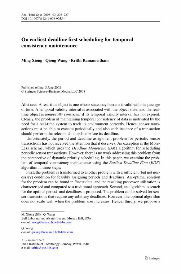
A time instant after which a transaction has the longest response time is calleda critical instant, e.g., time 0 is a critical instant for all transactions in DM if thosetransactions are synchronous (Leung and Whitehead 1982). To minimize the updateworkload, ML is used to guarantee temporal consistency with much less processorworkload than HH (Burns and Davis 1996; Xiong and Ramamritham 1999). In ML,Deadline Monotonic (DM) is used to schedule periodic sensor transactions. Thus werefer to this scheme as MLDM in the rest of the paper. There are three constraints torespect:

214 Real-Time Syst (2008) 40: 208–237

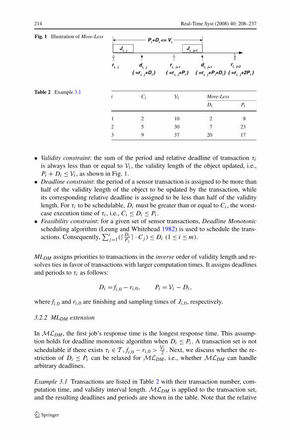
Fig. 1 Illustration of More-Less

Table 2 Example 3.1i Ci Vi More-Less

Di Pi

1 2 10 2 8

2 5 30 7 23

3 9 37 20 17

• Validity constraint: the sum of the period and relative deadline of transaction τi

is always less than or equal to Vi , the validity length of the object updated, i.e.,Pi + Di ≤ Vi , as shown in Fig. 1.

• Deadline constraint: the period of a sensor transaction is assigned to be more thanhalf of the validity length of the object to be updated by the transaction, whileits corresponding relative deadline is assigned to be less than half of the validitylength. For τi to be schedulable, Di must be greater than or equal to Ci , the worst-case execution time of τi , i.e., Ci ≤ Di ≤ Pi .

• Feasibility constraint: for a given set of sensor transactions, Deadline Monotonicscheduling algorithm (Leung and Whitehead 1982) is used to schedule the trans-actions. Consequently,

∑ij=1(�Di

Pj� · Cj) ≤ Di (1 ≤ i ≤ m).

MLDM assigns priorities to transactions in the inverse order of validity length and re-solves ties in favor of transactions with larger computation times. It assigns deadlinesand periods to τi as follows:

Di = fi,0 − ri,0, Pi = Vi − Di,

where fi,0 and ri,0 are finishing and sampling times of Ji,0, respectively.

3.2.2 MLDM extension

In M LDM , the first job’s response time is the longest response time. This assump-tion holds for deadline monotonic algorithm when Di ≤ Pi . A transaction set is notschedulable if there exists τi ∈ T , fi,0 − ri,0 >

Vi

2 . Next, we discuss whether the re-striction of Di ≤ Pi can be relaxed for M LDM , i.e., whether M LDM can handlearbitrary deadlines.

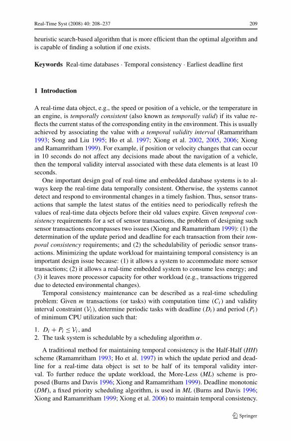
Example 3.1 Transactions are listed in Table 2 with their transaction number, com-putation time, and validity interval length. M LDM is applied to the transaction set,and the resulting deadlines and periods are shown in the table. Note that the relative

Real-Time Syst (2008) 40: 208–237 215

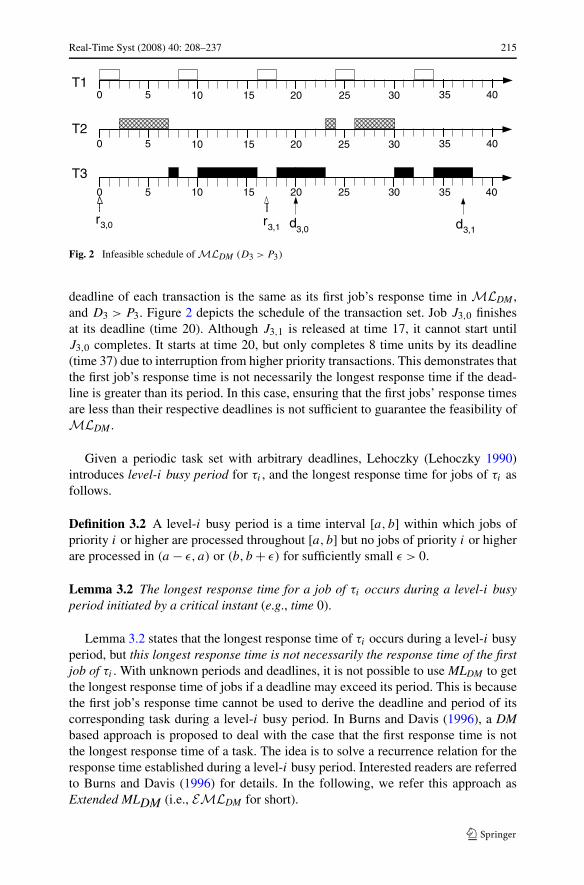
Fig. 2 Infeasible schedule of M LDM (D3 > P3)

deadline of each transaction is the same as its first job’s response time in M LDM ,and D3 > P3. Figure 2 depicts the schedule of the transaction set. Job J3,0 finishesat its deadline (time 20). Although J3,1 is released at time 17, it cannot start untilJ3,0 completes. It starts at time 20, but only completes 8 time units by its deadline(time 37) due to interruption from higher priority transactions. This demonstrates thatthe first job’s response time is not necessarily the longest response time if the dead-line is greater than its period. In this case, ensuring that the first jobs’ response timesare less than their respective deadlines is not sufficient to guarantee the feasibility ofM LDM .

Given a periodic task set with arbitrary deadlines, Lehoczky (Lehoczky 1990)introduces level-i busy period for τi , and the longest response time for jobs of τi asfollows.

Definition 3.2 A level-i busy period is a time interval [a, b] within which jobs ofpriority i or higher are processed throughout [a, b] but no jobs of priority i or higherare processed in (a − ε, a) or (b, b + ε) for sufficiently small ε > 0.

Lemma 3.2 The longest response time for a job of τi occurs during a level-i busyperiod initiated by a critical instant (e.g., time 0).

Lemma 3.2 states that the longest response time of τi occurs during a level-i busyperiod, but this longest response time is not necessarily the response time of the firstjob of τi . With unknown periods and deadlines, it is not possible to use MLDM to getthe longest response time of jobs if a deadline may exceed its period. This is becausethe first job’s response time cannot be used to derive the deadline and period of itscorresponding task during a level-i busy period. In Burns and Davis (1996), a DMbased approach is proposed to deal with the case that the first response time is notthe longest response time of a task. The idea is to solve a recurrence relation for theresponse time established during a level-i busy period. Interested readers are referredto Burns and Davis (1996) for details. In the following, we refer this approach asExtended MLDM (i.e., E M LDM for short).

216 Real-Time Syst (2008) 40: 208–237

4 Designing More-Less using EDF

This section presents a design for temporal consistency maintenance using EDFwhile Di ≤ Pi holds. Section 4.1 formulates an EDF optimization problem forDi ≤ Pi . Section 4.2 presents feasibility conditions for EDF scheduling. Section 4.3gives the design of ML using EDF by solving the optimization problem under a suf-ficient (but not necessary) feasibility condition.

4.1 Restricted optimization problem for ML using EDF

The optimized solution has to minimize processor workload U while maintaining thetemporal validity of real-time data in RTDBs. This essentially formalizes the follow-ing optimization problem that minimizes U with variables �P and �D. Note that �P , �D,�C, and �V given below are vectors.

Problem 4.1 Restricted EDF optimization problem: Given a set of transactions T ={τi}mi=1 with known �C and �V , determine �P and �D for synchronous transactions tominimize U , i.e.,

min�P , �D

U , where U =m∑

i=1

Ci

Pi

(1 ≤ i ≤ m),

subject to:

• Validity constraint: Pi + Di ≤ Vi .• Deadline constraint: Ci ≤ Di ≤ Pi .• Feasibility constraint: T with derived deadlines and periods is feasible by using

EDF scheduling.

As discussed, deadline constraint can be further generalized by having Ci ≤min(Di,Pi). In this section, Deadline constraint in Problem 4.1 is used for our dis-cussion unless specified otherwise. It is generalized in the next section. Next, we con-sider a sufficient feasibility condition for designing More-Less using EDF, namelyM LEDF . The corresponding feasibility test reduces the complexity of the problem.

4.2 Feasibility conditions for EDF

The periodic task model is a special case of the sporadic task model discussed inBaruah et al. (1990a, 1990b). A task τi in the sporadic task model is characterized bythree parameters—an execution time Ci , a deadline Di , and a minimum separationPi for the arrival time of two successive τi jobs, with Ci ≤ min(Di,Pi). If all jobsof a task arrive with the exact minimum separation Pi , this sporadic task becomes aperiodic task. Note that the arrival time of a task job is the same as the sampling timeof a sensor transaction job.

Real-Time Syst (2008) 40: 208–237 217

Given periodic task τi ∈ T (1 ≤ i ≤ m), processor demand bound functions, asexplained in Baruah et al. (1990a) are defined as follows:

Hi (t) = max

(

0,

(⌊t − Di

Pi

⌋

+ 1

)

· Ci

)

, (1)

HT (t) =m∑

i=1

Hi (t). (2)

Hi (t) represents the processor demand for τi on [0, t), i.e., the minimum amountof computation time that must be allocated for τi before time t . Similarly, HT (t)

represents the processor demand for all tasks in T on [0, t). The following lemma isfrom Lemma 3 in Baruah et al. (1990a) for a set of periodic transactions T .

Lemma 4.1 T is feasible iff HT (t) ≤ t for all t ≥ 0.

Lemma 4.1 will be used in Sect. 5 to derive solutions for EDF scheduling. Next,we present a technical result that is a sufficient condition for a set of periodic trans-actions T to be feasible using EDF scheduler (see Stankovic et al. 1998 for proof).

Lemma 4.2 Given a set of transactions T , if∑

τi∈TCi

min (Pi ,Di)≤ 1, then T is feasi-

ble. �

4.3 Designing M LEDF using a sufficient feasibility condition

In this section, we investigate the design of M LEDF using Lemma 4.2 for all τi withDi ≤ Pi . If Lemma 4.2 is used to derive deadlines and periods for T , the optimizationproblem for EDF scheduling is essentially transformed to the following problem.

Problem 4.2 EDF optimization problem with sufficient feasibility condition:

min�P

U , where U =m∑

i=1

Ci

Pi

(1 ≤ i ≤ m)

subject to:

• Validity and deadline constraints in Problem 4.1, and• Feasibility constraint:

∑mi=1

Ci

Di≤ 1.

It should be obvious that U is minimized only if Pi + Di = Vi . Otherwise, Pi

can always be increased and processor utilization can be decreased. Without loss ofgenerality, we assume that

Di = 1

Ni

Vi , (3)

Pi = Ni − 1

Ni

Vi , (4)

218 Real-Time Syst (2008) 40: 208–237

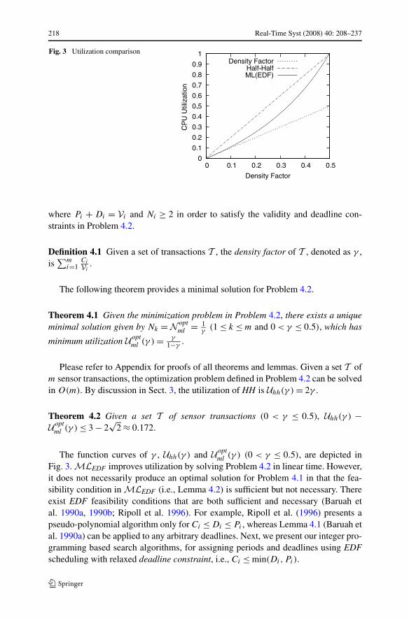
Fig. 3 Utilization comparison

where Pi + Di = Vi and Ni ≥ 2 in order to satisfy the validity and deadline con-straints in Problem 4.2.

Definition 4.1 Given a set of transactions T , the density factor of T , denoted as γ ,is

∑mi=1

Ci

Vi.

The following theorem provides a minimal solution for Problem 4.2.

Theorem 4.1 Given the minimization problem in Problem 4.2, there exists a uniqueminimal solution given by Nk = N opt

ml = 1γ

(1 ≤ k ≤ m and 0 < γ ≤ 0.5), which has

minimum utilization U optml (γ ) = γ

1−γ.

Please refer to Appendix for proofs of all theorems and lemmas. Given a set T ofm sensor transactions, the optimization problem defined in Problem 4.2 can be solvedin O(m). By discussion in Sect. 3, the utilization of HH is Uhh(γ ) = 2γ .

Theorem 4.2 Given a set T of sensor transactions (0 < γ ≤ 0.5), Uhh(γ ) −U opt

ml (γ ) ≤ 3 − 2√

2 ≈ 0.172.

The function curves of γ , Uhh(γ ) and U optml (γ ) (0 < γ ≤ 0.5), are depicted in

Fig. 3. M LEDF improves utilization by solving Problem 4.2 in linear time. However,it does not necessarily produce an optimal solution for Problem 4.1 in that the fea-sibility condition in M LEDF (i.e., Lemma 4.2) is sufficient but not necessary. Thereexist EDF feasibility conditions that are both sufficient and necessary (Baruah etal. 1990a, 1990b; Ripoll et al. 1996). For example, Ripoll et al. (1996) presents apseudo-polynomial algorithm only for Ci ≤ Di ≤ Pi , whereas Lemma 4.1 (Baruah etal. 1990a) can be applied to any arbitrary deadlines. Next, we present our integer pro-gramming based search algorithms, for assigning periods and deadlines using EDFscheduling with relaxed deadline constraint, i.e., Ci ≤ min(Di,Pi).

Real-Time Syst (2008) 40: 208–237 219

5 Designing search algorithms using EDF

This section presents algorithms—using the sufficient and necessary feasibility con-dition for EDF in Lemma 4.1—to search for optimal periods and deadlines of sensortransactions when arbitrary deadlines are allowed. Section 5.1 defines a general EDFoptimization problem with relaxed deadline constraint, i.e., Ci ≤ min(Di,Pi). Sec-tion 5.2 shows the optimality of EDF solutions compared to solutions produced byother periodic schedulers. Sections 5.3 and 5.4 present branch and bound based opti-mal and heuristic search algorithms, respectively, and show that the general problemcan be solved efficiently without reducing schedulability.

5.1 Formalizing the general EDF optimization problem

Following Lemma 4.1, Problem 4.1 can be generalized to the following problem.

Problem 5.1 General EDF optimization problem:

U optEDF = min

�P , �DU , where U =

m∑

i=1

Ci

Pi

subject to:

• Validity constraint: Pi + Di ≤ Vi .• Deadline constraint: Ci ≤ min(Di,Pi).• Feasibility constraint: ∀t, HT (t) ≤ t .

The problem of deciding whether sporadic task set T with arbitrary deadlines(i.e., Ci ≤ min(Di,Pi)) is feasible with given deadlines and periods is known to bein co-NP (Baruah et al. 1990a). The feasibility test for T with given deadlines andperiods is a sub-problem of the optimization problem in Problem 5.1, i.e., Problem5.1 contains a known co-NP problem.

By definition of (1) and (2),

HT (t) =m∑

i=1

max

(

0,

(⌊t − Di

Pi

⌋

+ 1

)

· Ci

)

. (5)

Note that the optimal solution can only be achieved when Pi + Di = Vi . Thus, Di =Vi −Pi , and considering the deadline constraint in Problem 5.1, we derive the periodconstraint as follows by replacing Di with Vi − Pi in the deadline constraint:

Ci ≤ Pi ≤ Vi − Ci. (6)

Replacing Di with Vi − Pi in (5), the feasibility constraint in Problem 5.1 is:

HT (t) =m∑

i=1

max

(

0,

(⌊(t − Vi )

Pi

⌋

+ 2

)

· Ci

)

≤ t. (7)

220 Real-Time Syst (2008) 40: 208–237

Equation (7) is also referred as time constraint. Thus, Problem 5.1 can be transformedinto minimizing U subject to the period constraint (6) and time constraint (7). Thereare no existing solutions for this problem, which is difficult since it has an unboundedvariable t . Next, we present a lemma that gives a bound on the “time length” neces-sary for determining the feasibility.

Lemma 5.1 Given a set of transactions T with U < 1, let

tB( �P ) = max

(

maxi

(Vi − 2Ci),

∑mi=1(2 − Vi

Pi)Ci

1 − U

)

.

T is feasible iff ∀t < tB( �P ), HT (t) ≤ t .

Lemma 5.1 indicates that a feasibility testing algorithm does not have to check∀t ≤ P, HT (t) ≤ t , where P is the least common multiple of all periods. Thus afeasibility testing algorithm based on Lemma 5.1 can run in pseudo-polynomial timefor a large percentage of sensor transaction sets, although it is exponential in theworst-case. Its complexity is similar to the feasibility testing algorithms in Baruah etal. (1990a), Ripoll et al. (1996). Note that Lemma 5.1 can only be applied when �Pis known. It cannot be applied to Problem 5.1 for feasibility test unless �P has beendetermined.

5.2 Optimality of EDF solutions

EDF is not the only scheduler that can be used to schedule periodic tasks. One openquestion is whether an optimal solution for Problem 5.1 minimizes utilization for allschedulers that can be used to derive periods and deadlines of T . Problem 5.1 can befurther generalized as follows.

Problem 5.2 General scheduler optimization problem:

min�P , �D

U , where U =m∑

i=1

Ci

Pi

subject to:

• Validity and deadline constraints in Problem 5.1.• Feasibility constraint: a periodic schedule from any scheduler that is feasible for

periodic transaction set T .

The following theorem shows optimality of EDF solutions.

Theorem 5.1 An optimized utilization of EDF solutions, U optEDF , of Problem 5.1 is

also optimal for Problem 5.2 in that if there exists a periodic schedule that is feasiblefor Problem 5.2 with utilization U , then U opt

EDF ≤ U .

Next, we present a search algorithm, which uses the branch and bound method ininteger programming, to find an optimal solution for EDF scheduling.

Real-Time Syst (2008) 40: 208–237 221

5.3 O S EDF : optimal search using EDF

This subsection presents our optimal search algorithm using EDF scheduling, namelyO S EDF . It finds optimal �P that minimizes processor utilization in Problem 5.1. Wefirst give the high-level algorithm, then define its constituents.

O S EDF is depicted in Algorithm 5.1. It first relaxes Problem 5.1 by defining aproxy problem that initially has no time constraint. It then solves the proxy problemand obtains a trial solution �P K (K = 0,1,2, . . .). A testing problem is defined to testif �P K satisfies all time constraints. If not, a new time constraint is added to tightenthe proxy problem. Then the algorithm iterates to solve the proxy problem again.This iteration continues until the trial solution �P K satisfies all time constraints, or theproxy problem becomes unsolvable.

Algorithm 5.1 O S EDF :

1. Define a relaxed version of Problem 5.1, namely the proxy problem (see Prob-lem 5.3). Problem 5.3 has no time constraint in the first iteration. A new timeconstraint is added at each iteration. Therefore, Problem 5.3 has only a limitednumber of time constraints in each iteration.

2. In the K th (K = 0,1,2, . . .) iteration, solve Problem 5.3 to obtain a trial solu-tion �P K . Since Problem 5.3 does not have all time constraints (in (7)), the utiliza-tion of its solution, U K , is no greater than that of the optimal solution to Problem5.1, U opt

EDF .3. Given trial solution �P K , solve the testing problem (see Problem 5.4). This de-

termines whether any time constraint (in (7)) is violated. If so, the solution toProblem 5.4 identifies a time point, tK , at which the time constraint is the tightestfor the given �P K (i.e., �P K exceeds the constraint to the largest extent at tK ). ThenProblem 5.3 is updated by adding a new time constraint at tK . The trial solution tothe updated Problem 5.3 in the next iteration is feasible for more time constraints(in (7)), or the problem becomes unsolvable.

4. Continue for Steps 2 and 3 until Problem 5.3 produces a solution that violates notime constraint in Problem 5.1, as determined by Problem 5.4.

The proxy problem in Algorithm 5.1 is defined as follows:

Problem 5.3 Proxy problem:

U K = min�z

m∑

i=1

Ci

Vi−Ci∑

j=Ci

zi,j

j(8)

subject to:

zi,j ∈ {0,1} andVi−Ci∑

j=Ci

zi,j = 1, (9)

m∑

i=1

Ci

Vi−Ci∑

j=Ci

zi,j · max

{

0,

⌊tk − Vi

j

⌋

+ 2

}

≤ tk, (10)

222 Real-Time Syst (2008) 40: 208–237

where i, j , and k are integers, and i = 1, . . . ,m, j = Ci, . . . , Vi − Ci, k = 1, . . . ,K .

U K is the minimized processor utilization at the K th iteration. Binary variable zi,j

determines the value of Pi between Ci and Vi − Ci(1 ≤ i ≤ m). Constraint (9) indi-cates that one and only one zi,j can be set to 1 for each τi . This implies that Pi = j

for zi,j = 1 (Ci ≤ j ≤ Vi − Ci). Note that

Vi−Ci∑

j=Ci

jzi,j = Pi, (11)

Vi−Ci∑

j=Ci

zi,j

j= 1

Pi

. (12)

Constraint (10) satisfies time constraints (7) at selected time points t = t1, . . . , tK . Inthe first iteration (i.e., K = 0), no time constraint is present. K is incremented in eachiteration afterwards. Hence, Problem 5.3 only has K time constraints as opposed toan infinite number of time constraints in Problem 5.1.

Lemma 5.2 demonstrates a relationship between Problems 5.1 and 5.3. It showsthat the optimal utilization of Problem 5.3 for each iteration (K = 1,2, . . . , ) consti-tutes a monotonically increasing sequence that is bounded by the optimal utilizationof Problem 5.1.

Lemma 5.2 Let �zK be an optimal solution to Problem 5.3 in the K th iteration. If U K

is the minimized utilization in (8) where zi,j = zKi,j (1 ≤ i ≤ m, Ci ≤ j ≤ Vi − Ci),

then

U 0 ≤ U 1 ≤ · · · ≤ U K ≤ U optEDF,

where U optEDF is the optimized utilization to Problem 5.1.

Lemma 5.2 implies that if �zK satisfies the time constraint at any t ≥ 0, then thecorresponding �P K must be an optimal solution to Problem 5.1. Hence the solutionobtained with Algorithm 5.1 has optimal utilization.

Considering (7), we define

F(t) = t −m∑

i=1

max

(

0,

(⌊t − Vi

Pi

⌋

+ 2

)

Ci

)

.

To determine whether �P K violates any time constraint, we examine the minimumF(t) in the K th iteration, namely FK . The time constraint is violated if FK < 0.This is formulated as an integer programming problem, namely the testing problem.

Problem 5.4 Testing problem:

FK = mint,�y≥0

[

t −m∑

i=1

max(0, (yi + 2)Ci)

]

(13)

Real-Time Syst (2008) 40: 208–237 223

subject to:

(t − Vi )

P Ki

− 1 ≤ yi ≤ (t − Vi )

P Ki

(1 ≤ i ≤ m), (14)

where t and �y are integer variables, and �P K , the trial solution from Problem 5.3 inthe same iteration, is an input parameter. Variable �y is introduced to remove the floorfunction in the definition of F(t).

Lemma 5.3 gives the rationale for formulating and solving Problem 5.4.

Lemma 5.3 Let �zK optimize Problem 5.3 in the K th iteration, and

P Ki =

Vi−Ci∑

j=Ci

jzi,j , i = 1, . . . ,m.

Then �P K is the optimal solution to Problem 5.1 if and only if FK ≥ 0.

It is noteworthy that Lemma 5.3 defines a stopping criterion, i.e., FK ≥ 0, forterminating the computation when an optimal solution is found. Further, if FK < 0,then the trial solution is infeasible for Problem 5.1. By definition of (13), the time atwhich FK reaches the minimum, denoted by tK , is the tightest time constraint where�P K exceeds the constraint to the largest extent. We add the time constraint at tK to

Problem 5.3 in the next iteration.Since there are only limited choices for zi,j (and thus Pi ) in Problem 5.3, the

iteration in Algorithm 5.1 ends up in one of two following situations: (1) FK inProblem 5.4 becomes non-negative, at which point an optimal solution is found (byLemma 5.3); (2) as more time constraints are added to (10), Problem 5.3 eventuallybecomes infeasible. This implies that there exists a subset of time constraints in (10)(thus, in (7)) that cannot be satisfied simultaneously. Note that O S EDF transformsProblem 5.1 to Problems 5.3 and 5.4, which are linear integer programming modelsthat can be solved by the branch and bound method Wolsey (1998) provided bycommercial optimization software, e.g., CPLEX.1

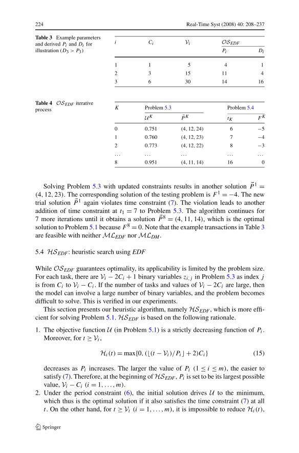
Illustration We demonstrate how Algorithm 5.1 works with the example in Table 3.Table 4 depicts the iterative process for finding an optimal solution for the transactionset in Table 3. Starting from K = 0 (i.e., the case of no time constraint), the solu-tion to Problem 5.3 is �P 0 = (4,12,24). Solving the testing problem (Problem 5.4),F 0 = −5. By Lemma 5.3, the solution violates the time constraint. The tightest timeconstraint occurs at t = 6, at which F 0 = −5. Therefore, the following time con-straint at t0 = 6 is added to Problem 5.3:

m∑

i=1

Ci

Vi−Ci∑

j=Ci

zi,j max

{

0,

⌊6 − Vi

j

⌋

+ 2

}

≤ 6.

1http://www.ilog.com/products/cplex

224 Real-Time Syst (2008) 40: 208–237

Table 3 Example parametersand derived Pi and Di forillustration (D3 > P3)

i Ci Vi O S EDF

Pi Di

1 1 5 4 1

2 3 15 11 4

3 6 30 14 16

Table 4 O S EDF iterativeprocess K Problem 5.3 Problem 5.4

U K �PK tK FK

0 0.751 (4,12,24) 6 −5

1 0.760 (4,12,23) 7 −4

2 0.773 (4,12,22) 8 −3

. . . . . . . . . . . . . . .

8 0.951 (4,11,14) 16 0

Solving Problem 5.3 with updated constraints results in another solution �P 1 =(4,12,23). The corresponding solution of the testing problem is F 1 = −4. The newtrial solution �P 1 again violates time constraint (7). The violation leads to anotheraddition of time constraint at t1 = 7 to Problem 5.3. The algorithm continues for7 more iterations until it obtains a solution �P 8 = (4,11,14), which is the optimalsolution to Problem 5.1 because F 8 = 0. Note that the example transactions in Table 3are feasible with neither M LEDF nor M LDM .

5.4 H S EDF : heuristic search using EDF

While O S EDF guarantees optimality, its applicability is limited by the problem size.For each task, there are Vi − 2Ci + 1 binary variables zi,j in Problem 5.3 as index j

is from Ci to Vi − Ci . If the number of tasks and values of Vi − 2Ci are large, thenthe model can involve a large number of binary variables, and the problem becomesdifficult to solve. This is verified in our experiments.

This section presents our heuristic algorithm, namely H S EDF , which is more effi-cient for solving Problem 5.1. H S EDF is based on the following rationale.

1. The objective function U (in Problem 5.1) is a strictly decreasing function of Pi .Moreover, for t ≥ Vi ,

Hi (t) = max{0, (�(t − Vi )/Pi� + 2)Ci} (15)

decreases as Pi increases. The larger the value of Pi (1 ≤ i ≤ m), the easier tosatisfy (7). Therefore, at the beginning of H S EDF , Pi is set to be its largest possiblevalue, Vi − Ci (i = 1, . . . ,m).

2. Under the period constraint (6), the initial solution drives U to the minimum,which thus is the optimal solution if it also satisfies the time constraint (7) at allt . On the other hand, for t ≥ Vi (i = 1, . . . ,m), it is impossible to reduce Hi (t),

Real-Time Syst (2008) 40: 208–237 225

since doing so requires increasing Pi above its upper bound Vi −Ci . Therefore, ifthe initial solution violates the time constraint (7) at t for t ≥ Vmax, where

Vmax = maxi

(Vi ), (16)

then the problem is infeasible.3. Lemma 5.1 is used to test if a given �P violates any time constraint. Specifically,

given �P , we calculate tB( �P) defined in the lemma. For each t ≤ tB( �P ), we evalu-ate Hi (t) according to (15). The summation of Hi (t) gives HT (t), which shouldnot exceed t . Otherwise the constraint (7) is infeasible under the current value of�P and an adjustment is required. Note that once �P is changed, the value of tB( �P)

is changed correspondingly.4. Suppose the test by Lemma 5.1 shows that the initial solution violates the time

constraint (7) at t ′, i.e., HT (t ′) > t ′. In this case, given set {τi : Ci ≤ t ′ < Vi −Ci}and Hi (t

′) definition (15),

Hi (t′) =

{0, Ci ≤ Pi < Vi − t ′,Ci, Vi − t ′ ≤ Pi ≤ Vi − Ci.

(17)

For transaction τi that satisfies Hi (t′) = Ci , Hi (t

′) can be reduced to 0 by settingPi = Vi − t ′ − 1 if Vi − t ′ − 1 ≥ Ci . Otherwise it violates the period constraint (6)at the lower end. Note that in Hi (t

′),

⌊t ′ − Vi

Pi

⌋⎧⎨

⎩

≥ 0 t ′ ≥ Vi ,

= −1 Pi ≥ Vi − t ′ and t ′ < Vi ,

≤ −2 Pi ≤ Vi − t ′ and t ′ < Vi .

(18)

These three cases of � t ′−Vi

Pi� are discussed below.

(a) � t ′−Vi

Pi� ≥ 0 implies that Hi (t

′) ≥ 2Ci . Reducing Pi increases Hi (t′). This

does not help reduce HT (t ′). Thus, Pi should not be changed.(b) � t ′−Vi

Pi� = −1 implies that Hi (t

′) = Ci . If Pi is reduced to Vi − t ′ − 1 ≥ Ci ,

then � t ′−Vi

Pi� = −2. In this case, Hi (t

′) is reduced to 0 from Ci . Thus, HT (t ′)is reduced.

(c) � t ′−Vi

Pi� ≤ −2 implies that Hi (t

′) = 0. If Pi is reduced, Hi (t′) stays 0 but U is

increased. So Pi should not be changed.Thus, Pi can only be changed in case (b). Let

R(t ′) ={

τi :⌊

t ′ − Vi

Pi

⌋

= −1 and Vi − t ′ − 1 ≥ Ci

}

(19)

be the set of transactions whose periods can be reduced to Vi − t ′ − 1. Note thatVi − t ′ − 1 ≥ Ci implies that

t ′ ≤ Vi − Ci − 1 ≤ Vi .

If R(t ′) has a sufficient number of transactions, then reducing periods of sometransactions may satisfy the time constraint (7) at t ′.

226 Real-Time Syst (2008) 40: 208–237

5. Nevertheless, reducing Pi always increases U . Specifically, if Pi (τi ∈ R(t ′)) isreduced to Vi − t ′ − 1, then U is increased by the following positive amount:

δi ≡ Ci

Vi − t ′ − 1− Ci

Pi

.

Reducing Pi not only affects the objective function U negatively, but also in-creases Hi (t) for time t > Vi , which tightens the time constraint (7) at thosepoints. Therefore, care needs to be taken to decide which transactions’ periods inR(t ′) should be reduced so that Hτ (t) is not overly increased for t > Vi , therebymaintaining Hτ (t) ≤ t . In H S EDF , transactions are selected from R(t ′) for reduc-ing their periods by solving the following selection problem.

Problem 5.5 Selection problem:

minwi : τi∈R(t ′)

m∑

i=1

wiδi (20)

subject to:

wi ∈ {0,1} and∑

i:τi∈R(t ′)Ciwi ≥ HT (t ′) − t ′, (21)

where wi : τi ∈ R(t ′) are binary variables.

By solving Problem 5.5, Pi (τi ∈ R(t ′)) is reduced to Vi − t ′ − 1 if wi = 1, or un-changed if wi = 0. Thus periods are reduced in a manner that the increment of U isminimized. Equation (21) eliminates the deficit of the time constraint, HT (t ′) − t ′,at t ′, which makes (7) feasible at t ′, i.e., HT (t ′) ≤ t ′. We consider Problem 5.1 infea-sible if Problem 5.5 is unsolvable. Each instance of Problem 5.5 is a Knapsack modelthat can be solved by CPLEX.

Algorithm 5.2 H S EDF :

1. Initialization: Pi = Vi − Ci, i = 1, . . . ,m. With the initial solution, the time con-straint is always satisfied at t = 0 as Hi (0) = 0. Set the starting time t = 1.

2. Calculate utilization U ( �P ) (Problem 5.1). Stop if U ( �P ) > 1, the problem is infea-sible.

3. Calculate tB( �P ) as given by Lemma 5.1.If t = tB( �P ), stop and return �P ∗ = �P as the final solution.

4. If HT (t) ≤ t , which means that �P does not violate (7) at t , set t = t + 1 and goto Step 3. Otherwise, solve Problem 5.5, reset Pi = Vi − t − 1 for τi ∈ R(t) withwi = 1, and go to Step 2. If Problem 5.5 is unsolvable, then stop—Problem 5.1 isinfeasible.

One salient feature of H S EDF is that it only checks each time point once: if thealgorithm reaches time t ′, it is not necessary to check feasibility for t < t ′ even if �Phas been changed at t ′. This property is supported by Theorem 5.2.

Real-Time Syst (2008) 40: 208–237 227

Theorem 5.2 Let T (t ′) be the transaction set with solution �P(t ′) obtained afterStep 4 in Algorithm 5.2 at time t ′ ≥ 0. Then T (t ′) with �P(t ′) satisfies the time con-straint at all t ≤ t ′. That is, let

HT (t ′)(t) =m∑

i=1

max

(

0,

(⌊(t − Vi )

Pi(t ′)

⌋

+ 2

)

· Ci

)

,

then HT (t ′)(t) ≤ t for t ≤ t ′.

Theorem 5.2 indicates only one pass is needed for each time point t in Algo-rithm 5.2. The selection problem is solved when the current solution violates the timeconstraint at t and R(t) is not empty, which requires t ≤ Vmax (16). Therefore, Al-gorithm 5.2 at most solves the selection problem Vmax times, although it may iteratetB( �P ∗) time points where �P ∗ is the final solution of Algorithm 5.2. At each iteration,Algorithm 5.2 tests feasibility condition HT (t) ≤ t .

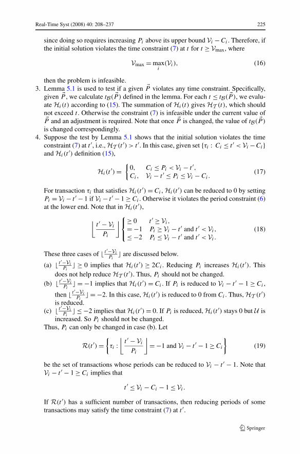
Illustration To illustrate H S EDF , the algorithm is applied to the example in Table 3.Table 5 shows the iteration process. At the starting point, �P = �V − �C = (4,12,24).As mentioned above, the solution always satisfies (7) at t = 0, so the algorithm startsat t = 1. The time constraint is first violated at t = 3, HT (t) exceeds t by 1. Applying�P and t ′ = 3 to (19), R(t ′) = {τ1, τ2}. At Step 4 of the algorithm,

P ′1 = V1 − t − 1 = 1, P ′

2 = V2 − t − 1 = 11,

δ1 = C1(1/P ′1 − 1/P1) = 0.75, δ2 = C2(1/P ′

2 − 1/P2) = 0.022.

This produces the following instance of Problem 5.5:

minw1,w2

{0.75w1 + 0.022w2 : w1 + 3w2 ≥ 1}. (22)

The solution is w1 = 0,w2 = 1. P2 is changed to 11 and P1 remains the same. It thenproceeds to t = 4. Once �P is changed, tB( �P ) also needs to be updated.

As t increments and the iteration continues, either (7) (HT (t) ≤ t) is verified tohold at t , in which case �P is unchanged, or the time constraint is violated and �P is

Table 5 H S EDF iterativeprocess t �P U HT (t) − t tB ( �P)

1 (4,12,24) 0.750 0 31

2 (4,12,24) 0.750 −1 31

3∗ (4,11,24) 0.773 1 32

4 (4,11,24) 0.773 0 32

. . . . . . . . . . . . . . .

15∗ (4,11,14) 0.951 1 38

. . . . . . . . . . . . . . .

38 (4,11,14) 0.951 −4 38

228 Real-Time Syst (2008) 40: 208–237

Table 6 O S EDF and H S EDFcomparison Algorithm O S EDF H S EDF

Variable# (∑m

i=1 (Vi − 2Ci + 1),m) m

Constraint# (K + m,m) 1

Iteration# K tB ( �P ∗)

Instance# K Vmax

updated. In Table 5, an asterisk is added as superscript in the first column for the lattercase. In these cases, HT (t) − t in the fourth column is calculated before the changeof the solution while �P in the second column is the new solution. Overall, �P hasbeen changed eight times before t = 15 at which point �P = (4,11,14). From time15 to tB( �P ) = 38, (7) is satisfied and �P remains unchanged. Following Lemma 5.1,no time constraint can be violated if t > tB( �P ) because

∑mi=1 Ci/Pi < 1. Therefore,

the algorithm stops at t = 38. Solution (4,11,14) is the same as that obtained withO S EDF . This demonstrates that H S EDF and O S EDF can schedule a larger set ofsensor transactions than existing approaches.

O S EDF vs. H S EDF : Table 6 compares numbers of variables (Var#) and constraints(Cons#) in Problems 5.3, 5.4, and 5.5. For O S EDF , the left number in a parenthesisrepresents Problem 5.3, while the right one represents Problem 5.4. The table alsocompares numbers of iterations (Iter#) in Algorithms 5.1 and 5.22 and along with op-timization problem instances solved by those algorithms (Inst#). O S EDF has signifi-cantly larger numbers of variables and constraints than H S EDF . This is why H S EDF

is more efficient than O S EDF , and O S EDF does not scale well with the problem size.The comparisons of numbers of iterations and solved optimization problem instancesare problem dependent. Note that H S EDF still involves solving the Knapsack prob-lem with the branch and bound method. Nevertheless, the number of variables islinear to the number of transactions.

Optimization for τi with Di > Pi Both Algorithms 5.1 and 5.2 enable EDF schedul-ing for transactions with deadline larger than period. Given transaction τi (1 ≤ i ≤ m)

with Di and Pi assigned by Algorithm 5.2 (or Algorithm 5.1), if Di > Pi , it is possi-ble to skip certain transaction jobs given the following lemma:

Lemma 5.4 (Job skipping) Given transaction τi (1 ≤ i ≤ m) with Di > Pi derivedfrom Algorithm 5.2, and jobs Ji,j and Ji,j+1 (j ≥ 0), if Ji,j cannot be started beforeri,j+1, then Ji,j can be skipped and Ji,j+1 can be executed in [ri,j+1,di,j ] while thevalidity constraint is guaranteed.

6 Performance evaluation

This section presents important results from our experimental studies of the proposedH S EDF and M LEDF algorithms.

2Note that �P ∗ is the final solution in Algorithm 5.2.

Real-Time Syst (2008) 40: 208–237 229

Table 7 Experimentalparameters and settings Parameter meaning Value

No. of CPU 1

No. of real-time data objects [50, 300]

Validity interval of data objects (ms) [4000, 8000]

CPU time per data access (ms) [5, 15]

Update transaction length 1

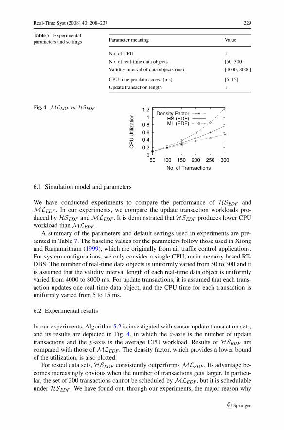
Fig. 4 M LEDF vs. H S EDF

6.1 Simulation model and parameters

We have conducted experiments to compare the performance of H S EDF andM LEDF . In our experiments, we compare the update transaction workloads pro-duced by H S EDF and M LEDF . It is demonstrated that H S EDF produces lower CPUworkload than M LEDF .

A summary of the parameters and default settings used in experiments are pre-sented in Table 7. The baseline values for the parameters follow those used in Xiongand Ramamritham (1999), which are originally from air traffic control applications.For system configurations, we only consider a single CPU, main memory based RT-DBS. The number of real-time data objects is uniformly varied from 50 to 300 and itis assumed that the validity interval length of each real-time data object is uniformlyvaried from 4000 to 8000 ms. For update transactions, it is assumed that each trans-action updates one real-time data object, and the CPU time for each transaction isuniformly varied from 5 to 15 ms.

6.2 Experimental results

In our experiments, Algorithm 5.2 is investigated with sensor update transaction sets,and its results are depicted in Fig. 4, in which the x-axis is the number of updatetransactions and the y-axis is the average CPU workload. Results of H S EDF arecompared with those of M LEDF . The density factor, which provides a lower boundof the utilization, is also plotted.

For tested data sets, H S EDF consistently outperforms M LEDF . Its advantage be-comes increasingly obvious when the number of transactions gets larger. In particu-lar, the set of 300 transactions cannot be scheduled by M LEDF , but it is schedulableunder H S EDF . We have found out, through our experiments, the major reason why

230 Real-Time Syst (2008) 40: 208–237

H S EDF outperforms M LEDF in terms of CPU utilization is due to the more accurateschedulability condition in Lemma 4.1. We have also done experiments with para-meter settings different from Table 7. The results are similar to what is depicted inFig. 4.

Other experiments We conducted experiments for the comparison of M LDM ,E M LDM and H S EDF . We found out that these algorithms produce about the sameCPU workload if the set of sensor transactions are schedulable by all the algorithms,but H S EDF and E M LDM can schedule a slightly larger set of sensor transactions dueto the fact that H S EDF allows arbitrary deadlines. However, it is difficult to quantifyhow much they can improve the feasibility of M LDM as the workload generationplays an important role in such a comparison. This issue needs further investigation,which is left as future work.

We also conducted another set of experiments by replacing the deadline constraintin Problem 5.1 with Ci ≤ Di ≤ Pi , i.e., deadlines are not greater than their corre-sponding periods. Then the H S EDF algorithm is slightly adjusted for the revisedproblem. Compared to H S EDF to Problem 5.1, there is little difference for the CPUutilization resulting from H S EDF for both problems. This indicates that the relaxationof the deadline constraint has little impact on the resulted CPU utilization of transac-tions. It only slightly improves the set of sensor transactions that can be scheduled.

7 Conclusions

Consistency maintenance of data is an important problem in real-time applications.We have proposed three novel approaches, namely M LEDF , O S EDF and H S EDF , us-ing the EDF scheduling algorithm. M LEDF is a linear algorithm but it only supportstransactions with deadlines no greater than their corresponding periods (i.e., Di ≤ Pi

for τi ). Our analysis for M LEDF in Sect. 4.3 sheds light on how much M LEDF canimprove over existing HH approach quantitatively. The other two approaches out-perform M LEDF as they are derived from processor demand analysis (Lemma 4.1),a more accurate feasibility condition for EDF scheduling. This is clearly demon-strated in our experimental results. In contrast, O S EDF and H S EDF support trans-actions with arbitrary deadlines. In particular, O S EDF is an algorithm that yieldsminimized processor utilization for periodic sensor transactions although it is not asefficient as the heuristic algorithm H S EDF . Our experimental results demonstrate thatH S EDF is an effective algorithm that assigns periods and deadlines with much lowerutilization than M LEDF .

However, more investigation is necessary to understand the performance differ-ence of the alternate approaches studied in this paper. In particular, we need to betterunderstand how HSEDF performs in comparison to EMLDM . For scheduling transac-tions with arbitrary deadlines, one of the important open questions is whether thereis any sufficient and necessary condition for schedulability of EDF in temporal con-sistency maintenance. Further investigation on those questions will help shed light onexisting approaches for temporal consistency maintenance.

Real-Time Syst (2008) 40: 208–237 231

Appendix

Proof of Theorem 4.1 From the deadline constraint in Problem 4.2, we have

Pi ≥ Di �⇒ Ni − 1

Ni

Vi ≥ 1

Ni

Vi �⇒ Ni ≥ 2,

Di ≥ Ci �⇒ Vi

Ci

≥ Ni.

Following equations (3) and (4), Problem 4.2 is reduced to the following non-linearprogramming problem with variable �N :

min�N

U , where U =m∑

i=1

NiCi

(Ni − 1)Vi

(1 ≤ i ≤ m)

subject to:

Ni ≥ 2, (23)

Vi

Ci

≥ Ni, (24)

m∑

i=1

Ni · Ci

Vi

≤ 1. (25)

It can be proved that the objective function and all three constraints are convex func-tions. Thus this is a convex programming problem, and a local minimum is a globalminimum for this problem (Hiller and Lieberman 1990). Considering (25) and (23)together, we have 2 · ∑m

i=1Ci

Vi≤ ∑m

i=1 Ni · Ci

Vi≤ 1. That is,

m∑

i=1

Ci

Vi

≤ 1

2. (26)

Equation (26) implies that γ ≤ 12 .

For convenience, let wi = Ci

Vi, γ = ∑m

i=1Ci

Vi= ∑m

i=1 wi, xi = Ni − 1. By defini-

tion of U and (4), U = ∑mi=1

NiCi

(Ni−1)Vi= ∑m

i=1xi+1xi

wi , i.e., U = ∑mi=1 wi +∑m

i=1wi

xi.

Following equations (23), (24) and (25), the problem is transformed to:

min�x

m∑

i=1

wi

xi

subject to:

xi − 1 ≥ 0, (27)

1

wi

− xi − 1 ≥ 0, (28)

232 Real-Time Syst (2008) 40: 208–237

1 − γ −m∑

i=1

wi · xi ≥ 0. (29)

Introducing Lagrangian multipliers λ1,i , λ2,i and λ3, we write Kuhn-Tucker conditionas following (1 ≤ i ≤ m):

−wi

x2i

+ λ3wi − λ2,i + λ1,i = 0, (30)

λ3

(

1 − γ −m∑

i=1

wixi

)

= 0, (31)

λ3 ≥ 0, (32)

λ2,i (xi − 1) = 0, (33)

λ2,i ≥ 0, (34)

λ1,i

(1

wi

− xi − 1

)

= 0, (35)

λ1,i ≥ 0. (36)

We use above conditions to construct an optimal solution. Suppose λ1,i = λ2,i = 0and λ3 > 0. Following equation (30), −wi

x2i

+ λ3wi = 0. Therefore, xi = 1√λ3

(λ3 >

0 and 1 ≤ i ≤ m). Following λ3 > 0 and (31), we have

1 − γ −m∑

i=1

wixi = 0.

Replacing xi with 1√λ3

,

1 − γ − 1√λ3

m∑

i=1

wi = 0.

Replacing∑m

i=1 wi with γ ,

1 − γ − 1√λ3

γ = 0.

Solving the above equation, we have λ3 = (γ

1−γ)2. It is easy to check that

λ1,i = λ2,i = 0, λ3 =(

γ

1 − γ

)2

and xi = 1√λ3

= 1 − γ

γ

satisfy (27) through (36), which means that �x reaches a local minimum. Because theobjective function is convex and constraints are all linear, �x is also a global optimalsolution. Since Ni = xi + 1, U is minimized when Ni = N opt

ml = 1γ

, and the minimum

utilization is U optml (γ ) = N opt

ml

N optml −1

∑mi=1

Ci

Vi=

1γ

1γ

−1γ = γ

1−γ. �

Real-Time Syst (2008) 40: 208–237 233

Proof of Theorem 4.2 Let D(γ ) = Uhh(γ ) − U optml (γ ). From definitions of U opt

ml (γ )

and Uhh(γ ), it follows that D(γ ) = 2γ − γ1−γ

. To obtain the maximum of D(γ ), wedifferentiate D(γ ) with respect to γ , and set the result to 0:

dD(γ )

dγ= 2γ 2 − 4γ + 1

(1 − γ )2= 0.

Thus the maximum of D(γ ) is 3 − 2√

2 when γ = 1 −√

22 . �

Proof of Lemma 5.1 If T is not feasible, then HT (t) > t (Lemma 4.1). We need tofind the maximal time t = tB( �P ) so that HT (t) > t may hold in [0, tB( �P)). BecausePi ≥ Ci , if

t ≥ maxi

(Vi − 2Ci), (37)

then (� (t−Vi )Pi

� + 2) ≥ 0 (Remember that Pi ≥ Ci ). Suppose (37) holds, we have

HT (t) =m∑

i=1

max

(

0,

(⌊(t − Vi )

Pi

⌋

+ 2

)

· Ci

)

=m∑

i=1

(⌊t − Vi

Pi

⌋

+ 2

)

· Ci

)

{Eliminating the max function}

≤m∑

i=1

Ci

Pi

t +m∑

i=1

Ci

(

2 − Vi

Pi

)

{Eliminating the floor function}.

If

t

m∑

i=1

Ci

Pi

+m∑

i=1

Ci

(

2 − Vi

Pi

)

≤ t, (38)

then HT (t) ≤ t . Solving (38), we have

t ≥∑m

i=1(2 − Vi

Pi)Ci

1 − ∑mi=1

Ci

Pi

.

Considering (37), we have HT (t) ≤ t if

t ≥ max

(

maxi

(Vi − 2Ci),

∑mi=1(2 − Vi

Pi)Ci

1 − U

)

.

Following Lemma 4.1, T is feasible iff ∀t < tB( �P ), HT (t) ≤ t . �

Proof of Theorem 5.1 Given a solution K of Problem 5.2 with deadlines and periodsderived from a scheduler S , suppose that utilization of K is UK , and UK < U opt

EDF . Kis feasible if it is scheduled by S . Since EDF is an optimal scheduler (Stankovic et

234 Real-Time Syst (2008) 40: 208–237

al. 1998), if K can be scheduled by S then it can also be scheduled by EDF. Thus,K is also a feasible solution for Problem 5.1. But UK < U opt

EDF contradicts that U optEDF

is the optimized (minimized) utilization for Problem 5.1. Thus U optEDF is optimal for

Problem 5.2. �

Proof of Lemma 5.2: First, we prove that U K ≤ U optEDF . Suppose �P ∗ is the optimal

solution to Problem 5.1, then P ∗i (i = 1, . . . ,m) is an integer between Ci and Vi −Ci

that can be expressed as

P ∗i =

Vi−Ci∑

j=Ci

jz∗i,j ,

where z∗i,j = 1 if j = P ∗

i ; otherwise, z∗i,j = 0. Note that

1

P ∗i

=Vi−Ci∑

j=Ci

z∗i,j

j. (39)

For any k = 0,1, . . . ,K , z∗i,j (Ci ≤ j ≤ Vi − Ci) (which determines �P ∗) is thus a

feasible solution to Problem (5.3) because (1) �P ∗ satisfies Constraint (9); (2) the setof time constraints of Problem 5.3 (Constraint (10)) is a subset of that of Problem 5.1(7). Following equation (10),

m∑

i=1

Ci

Vi−Ci∑

j=Ci

z∗i,j max

(

0,

⌊tk − Vi

j

⌋

+ 2

)

=m∑

i=1

max

(

0,

(⌊tk − Vi

P ∗i

⌋

+ 2

)

Ci

)

{Moving Ci and z∗i,j into the max function, and by (39)}

≤ tk {P ∗i satisfying (7)}.

By definition of Problem 5.3, all feasible solutions that satisfy Problem 5.3, zi,j = zKi,j

produces the minimum U K . Therefore, U K ≤ U optEDF .

We can prove that U n−1 ≤ U n (1 ≤ n ≤ K) similarly. �

Proof of Lemma 5.3 1. (If ) By the definition of FK , if FK ≥ 0 then

t ≥m∑

i=1

max

{

0,

(⌊t − Vi

P Ki

⌋

+ 2

)

Ci

}

.

This implies that (7) holds. So �P K satisfies both the period and time constraintsin Problem 5.1. By Lemma 5.2, U K ≤ U opt

EDF . Thus �P K also minimizes processorutilization in Problem 5.1, and it is an optimal solution.

2. (Only if ) This can be proved in a manner similar to the if case. �

Real-Time Syst (2008) 40: 208–237 235

Proof of Theorem 5.2 If �P (t ′) is obtained after Step 4 in Algorithm 5.2 at time t ′ ≥0, then HT (t ′)(t ′) ≤ t ′ for �P(t ′)’s corresponding transaction set T (t ′). First, �P(0)

must be feasible for the time constraint at t ′ = 0. Otherwise, the selection problem isunsolvable and the algorithm is terminated, which is contradictory to the assumptionthat �P(t ′) is obtained after Step 4 at time t ′ ≥ 0.

Suppose that �P(t ′) satisfies the time constraint at all t ≤ t ′, i.e., HT (t ′)(t) ≤ t . If�P(t ′) also satisfies HT (t ′)(t ′ + 1) ≤ t ′ + 1 at time t ′ + 1, then set �P(t ′ + 1) = �P(t ′)

and HT (t ′)(t) ≤ t holds for t ∈ [0, t ′ + 1]. Otherwise, Pi(t′) (τi ∈ R(t ′)) is reduced,

and �P(t ′) is changed to �P(t ′ + 1), which satisfies the time constraint at t ′ + 1 (byStep 4). Furthermore, Pi is only changed for τi ∈ R(t ′). By R(t ′) definition (19), wehave

Pi(t′ + 1) = Pi(t

′) if t ′ + 1 ≥ Vi , (40)

Pi(t′ + 1) ≤ Pi(t

′) if t ′ + 1 < Vi . (41)

Given t < t ′ + 1 and the definition of HT (t ′+1)(t),

HT (t ′+1)(t)

=m∑

i=1

max

(

0,

(⌊(t − Vi )

Pi(t ′ + 1)

⌋

+ 2

)

· Ci

)

≤m∑

i=1

max

(

0,

(⌊(t − Vi )

Pi(t ′)

⌋

+ 2

)

· Ci

)

{By (40), (41), and t − Vi < 0 if t ′ + 1 < Vi}

= HT (t ′)(t)

≤ t {By induction assumption}.

Therefore, for all t ≤ t ′ + 1, HT (t ′+1)(t) ≤ t , which proves the theorem. �

Proof of Lemma 5.4 Note that Ji,j is guaranteed by EDF scheduling to completeby di,j (note that ri,j+1 < di,j if Di > Pi ). If it cannot be executed before timeri,j+1, then it will have Ci time units allocated from the processor for its executionin [ri,j+1,di,j ]. Such Ci time units can also be used by Ji,j+1 if Ji,j is skipped. �

References

Baruah SK, Mok AK, Rosier LE (1990a) Preemptively scheduling hard-real-time sporadic tasks on oneprocessor. IEEE Real-Time Syst Symp, December1990

Baruah SK, Howell RR, Rosier LE (1990b) Algorithms and complexity concerning the preemptivescheduling of periodic, real-time tasks on one processor. Real-Time Syst 2(4):301–324

Burns A, Davis R (1996) Choosing task periods to minimise system utilisation in time triggered systems.Inf Process Lett 58:223–229

Gerber R, Hong S, Saksena M (1994) Guaranteeing end-to-end timing constraints by calibrating interme-diate processes. IEEE Real-Time Syst Symp, December 1994

236 Real-Time Syst (2008) 40: 208–237

Gustafsson T, Hansson J (2004a) Data management in real-time systems: a case of on-demand updates invehicle control systems. In: IEEE real-time and embedded technology and applications symposium,pp 182–191

Gustafsson T, Hansson J (2004b) Dynamic on-demand updating of data in real-time database systems. In:ACM SAC 2004

Hiller FS, Lieberman GJ (1990) Introduction to operations research. McGraw-Hill, New YorkKang KD, Son S, Stankovic JA, Abdelzaher T (2002) A QoS-sensitive approach for timeliness and fresh-

ness guarantees in real-time databases. In: EuroMicro real-time systems conference, June 2002Kuo T, Mok AK (1992) Real-time data semantics and similarity-based concurrency control. IEEE Real-

Time Syst Symp, December 1992Kuo T, Mok AK (1993) SSP: a semantics-based protocol for real-time data access. IEEE Real-Time Syst

Symp, December 1993Ho S, Kuo T, Mok AK (1997) Similarity-based load adjustment for static real-time transaction systems.

IEEE Real-Time Syst SympLehoczky JP (1990) Fixed priority scheduling of periodic task sets with arbitrary deadlines. IEEE Real-

Time Syst SympLiu CL, Layland J (1973) Scheduling algorithms for multiprogramming in a hard real-time environment.

J Assoc Comput Mach 20(1):46–61Leung J, Whitehead J (1982) On the complexity of fixed-priority scheduling of periodic real-time tasks.

Perform Eval 2:237–250Ramamritham K (1993) Real-time databases. Distributed and Parallel Databases 1(1993):199–226Ripoll I, Crespo A, Mok A (1996) Improvement in feasibility testing for real-time tasks. Real-Time Syst

11(1):19–39Seto D, Lehoczky JP, Sha L, Shin KG (1996) On task schedulability in real-time control systems. IEEE

Real-Time Syst Symp, December 1996Seto D, Lehoczky JP, Sha L (1998) Task period selection and schedulability in real-time systems. IEEE

Real-Time Syst Symp, December 1998Song X, Liu JWS (1995) Maintaining temporal consistency: pessimistic vs. optimistic concurrency control.

IEEE Trans Knowl Data Eng 7(5):786–796Stankovic JA, Spuri M, Ramamritham K, Buttazzo GC (1998) Deadline scheduling for real-time systems:

EDF and related algorithms. Kluwer Academic, DordrechtWolsey LA (1998) Integer programming. Wiley, New YorkXiong M, Ramamritham K (1999) Deriving deadlines and periods for real-time update transactions. IEEE

Real-Time Syst SympXiong M, Ramamritham K, Stankovic J, Towsley D, Sivasankaran RM (2002) Scheduling transactions

with temporal constraints: exploiting data semantics. IEEE Trans Knowl Data Eng 14(5):1155–1166Xiong M, Han S, Lam KY (2005) A deferrable scheduling algorithm for real-time transactions maintaining

data freshness. IEEE Real-Time Syst SympXiong M, Liang B, Lam K, Guo Y (2006) Quality of service guarantee for temporal consistency of real-

time transactions. IEEE Trans Knowl Data Eng 18(8):1097–1110

Ming Xiong received his Ph.D. degree in Computer Science from Uni-versity of Massachusetts Amherst in 2000. He is currently a memberof technical staff at Bell Labs. His research interests include databasesystems, real-time systems and mobile computing.

Real-Time Syst (2008) 40: 208–237 237

Qiong Wang received his Ph.D. in Engineering and Public Policy fromCarnegie-Mellon University in 1998. He is a member of Technical Staffat Bell Labs, where he works on topics on operations research, businessmathematics, and network economics.

Krithi Ramamritham received the Ph.D. in Computer Science fromthe University of Utah and then joined the University of Massachusetts.He is currently at the Indian Institute of Technology Bombay as theVijay and Sita Vashee Chair Professor in the Department of ComputerScience and Engineering. He is currently serving as Dean (R&D) ofIITB.Ramamritham’s interests span the areas of real-time systems, databasesystems, and real-time database systems. He is applying concepts fromthese areas to solve problems in embedded systems, mobile computing,e-commerce, intelligent internet, and the Web. During the last few yearshe has been interested in the use of Information and CommunicationTechnologies for creating tools aimed at socio-economic development.He is an Editor-in-Chief of the Real-Time Systems Journal. His othereditorial board contributions include IEEE Transactions on Knowledge

and Data Engineering, IEEE Transactions on Parallel and Distributed Systems, IEEE Transactions on Mo-bile Computing, IEEE Internet Computing, the WWW Journal, the Distributed and Parallel Databasesjournal, and the VLDB Journal.He has co-authored two IEEE tutorial texts on real-time systems, a text on advances in database transactionprocessing, and a text on scheduling in real-time systems.Prof. Ramamritham is a Fellow of the IEEE, a Fellow of the ACM, and a Fellow of the Indian NationalAcademy of Engineering.He received the Distinguished Alumnus Award from IIT Madras in 2006 and the Doctor of Science (Hon-oris Causa) from the University of Sydney in 2007.