Contents lists available at ScienceDirect

Journal of the Mechanics and Physics of Solids

Journal of the Mechanics and Physics of Solids 83 (2015) 263–284

http://d0022-50

n CorrE-m

journal homepage: www.elsevier.com/locate/jmps

Dielectric elastomer composites: A general closed-formsolution in the small-deformation limit

Stephen A. Spinelli, Victor Lefèvre, Oscar Lopez-Pamies n

Department of Civil and Environmental Engineering, University of Illinois, Urbana–Champaign, IL 61801, USA

a r t i c l e i n f o

Article history:Received 27 August 2014Received in revised form29 April 2015Accepted 13 June 2015Available online 18 June 2015

Keywords:ElectrostrictionElectroactive materialsMicrostructuresIterated homogenization

x.doi.org/10.1016/j.jmps.2015.06.00996/& 2015 Elsevier Ltd. All rights reserved.

esponding author.ail addresses: sspinel2@illinois.edu (S.A. Spin

a b s t r a c t

A solution for the overall electromechanical response of two-phase dielectric elastomercomposites with (random or periodic) particulate microstructures is derived in the clas-sical limit of small deformations and moderate electric fields. In this limit, the overallelectromechanical response is characterized by three effective tensors: a fourth-ordertensor describing the elasticity of the material, a second-order tensor describing its per-mittivity, and a fourth-order tensor describing its electrostrictive response. Closed-formformulas are derived for these effective tensors directly in terms of the correspondingtensors describing the electromechanical response of the underlying matrix and theparticles, and the one- and two-point correlation functions describing the microstructure.This is accomplished by specializing a new iterative homogenization theory in finiteelectroelastostatics (Lopez-Pamies, 2014) to the case of elastic dielectrics with even cou-pling between the mechanical and electric fields and, subsequently, carrying out thepertinent asymptotic analysis.

Additionally, with the aim of gaining physical insight into the proposed solution andshedding light on recently reported experiments, specific results are examined andcompared with an available analytical solution and with new full-field simulations for thespecial case of dielectric elastomers filled with isotropic distributions of spherical particleswith various elastic dielectric properties, including stiff high-permittivity particles, liquid-like high-permittivity particles, and vacuous pores.

& 2015 Elsevier Ltd. All rights reserved.

1. Introduction

The object of this paper is to generate a rigorous analytical solution for the overall or macroscopic electromechanicalresponse of dielectric elastomer composites with (random or periodic) particulate microstructures in the limit of smalldeformations and moderate electric fields. At a microscopic level, a dielectric elastomer composite is taken to consist of astatistically uniform distribution of particles bonded perfectly to a continuous matrix phase. The domain occupied by theentire composite in its (undeformed and stress-free) ground state is denoted byΩ. We assume that the characteristic lengthscale of the underlying particles is much smaller than the size of Ω and, for convenience, choose units of length so that Ωhas unit volume. The constitutive behaviors of the matrix (r¼1) and the particles (r¼2) are characterized by “total” freeenergies W r( ) that are objective functions of the deformation gradient tensor F and objective and even functions of theLagrangian electric field E so that W W WQF E F E F E, , ,r r r( ) = ( ) = ( − )( ) ( ) ( ) for all OrthQ ∈ +. At each material point X∈Ω, the

elli), vlefevre@illinois.edu (V. Lefèvre), pamies@illinois.edu (O. Lopez-Pamies)

S.A. Spinelli et al. / J. Mech. Phys. Solids 83 (2015) 263–284264

first Piola–Kirchhoff stress tensor S and the Lagrangian electric displacement field D are hence given by (Dorfmann andOgden, 2005; see also Suo et al., 2008)

W WS

FX F E D

EX F E, , and , , 1= ∂

∂( ) = − ∂

∂( ) ( )

with

W W WX F E X F E X F E, , 1 , , , 22 1 2 2θ θ( ) = [ − ( )] ( ) + ( ) ( ) ( )( ) ( ) ( ) ( )

where θ(2) X( ) stands for the indicator function of the regions occupied by the particles: θ(2) X( )¼1 if X is inside a particle andθ(2) X( )¼0 otherwise.

For random microstructures, the indicator function 2θ( ) in (2) is known only in a probabilistic sense. For periodic mi-crostructures, on the other hand, 2θ( ) is completely known once a unit cell and the lattice over which it is repeated arespecified. In either case, at any rate, we shall require but partial knowledge of 2θ( ) in terms of the one- and two-pointcorrelation functions. In view of the assumed statistical uniformity of the microstructure, these functions are insensitive totranslations and thus given by (see, e.g., Chapter 15 in Milton, 2002 and references therein)

p pX X Y Y X X Xd and d . 32 2 22 2 2∫ ∫θ θ θ= ( ) ( ) = ( + ) ( ) ( )Ω Ω

( ) ( ) ( ) ( ) ( )

Geometrically, the one-point correlation function p 2( ) represents the probability that a point lands in a particle when it isdropped randomly in Ω. In other words, p 2( ) is nothing more than the volume fraction of particles in the undeformedconfiguration; henceforth, we shall utilize the standard notation p c2 =( ) . The two-point correlation function p 22( ) representsthe probability that the ends of a rod of length and orientation described by the vector Y land within (the same or twodifferent) particles when dropped randomly in Ω. Accordingly, p 22( ) contains finer information about the size, shape, andspatial distribution of the particles in the undeformed configuration.

Granted the statistical uniformity of the microstructure and the separation between microscopic and macroscopic lengthscales, the overall constitutive response for the composite is defined as the relation between the volume averages of the firstPiola–Kirchhoff stress S S X Xd∫≐ ( )

Ωand electric displacement D D X Xd∫≐ ( )

Ωand the volume averages of the deformation

gradient F F X Xd∫≐ ( )Ω

and electric field E E X Xd∫≐ ( )Ω

over the undeformed configuration Ω when the composite issubjected to affine boundary conditions. Such a relation can be compactly written as (Lopez-Pamies, 2014)

Wc

WcS

FF E D

EF E, , and , , , 4= ∂

∂( ) = − ∂

∂( ) ( )

where

W c WF E X F E X, , min max , , d , 5F E∫( ) = ( ) ( )Ω∈ ∈

the effective free energy function, corresponds physically to the total electroelastic free energy (per unit undeformed vo-lume) of the composite. In these last expressions, the volume fraction of particles c has been included as an explicit ar-gument in the effective energy W for later convenience and and denote sufficiently large sets of admissible deformationgradients F and curl-free electric fields E with prescribed volume averages F and E, respectively. For later reference, we notethat the effective free energy function (5) is, by definition, objective in F and objective and even in E, namely,W c W c W cF E Q F E F E, , , , , ,( ) ( ) ( )= = − for all OrthQ ∈ +, much like its local counterpart (2).

1.1. The classical limit of small deformations and moderate electric fields

The focus of this paper is on the classical limit of small macroscopic deformations and moderate macroscopic electric fields.More precisely, defining ζ as a vanishingly small parameter, the deformation measure H F I≐ − , with I denoting the identityin the space of second-order tensors, is assumed to be O ζ( ) while the electric field E is assumed to be O 1/2ζ( ) (see, e.g.,Stratton, 1941; Toupin, 1956; Tian et al., 2012). In this limit, the effective free energy function (5) takes the asymptotic form

W c H L c H E c E H M c E E E E c E E OF E, ,12

12

, 6ij ijkl kl i ij j ij ijkl k l i j ijkl k l3τ ζ( ) = ( ) − ϵ ( ) + ( ) − ( ) + ( ) ( )

∼ ∼∼

where L∼stands for the effective modulus of elasticity, ϵ∼ denotes the effective permittivity, M is the effective electrostrictive

tensor, and τ∼ represents the effective permittivity of second order. Because of the energy character and overall objectivity ofthe definition (5), these tensors exhibit the symmetries L L L Lijkl klij jikl ijlk= = =

∼ ∼ ∼ ∼, ij jiϵ = ϵ∼ ∼ , M M Mijkl jikl ijlk= = , ijkl jiklτ τ= =∼ ∼

kjil ljki ikjl ilkj ijlkτ τ τ τ τ= = = =∼ ∼ ∼ ∼ ∼ . The corresponding relations for the macroscopic stress and electric displacement (4) reduce to

SWF

c L c H M c E E OF E, ,7

ijij

ijkl kl ijkl k l2ζ= ∂

∂( ) = ( ) + ( ) + ( )

( )∼

and

S.A. Spinelli et al. / J. Mech. Phys. Solids 83 (2015) 263–284 265

DWE

c c E OF E, , ,8i

iij j

3/2ζ= − ∂∂

( ) = ϵ ( ) + ( )( )

∼

to leading order. Here, it is important to recognize that the asymptotic constitutive relation (7) for the stress is O ζ( ) while theasymptotic constitutive relation (8) for the electric displacement is of different order, O 1/2ζ( ). It is also important to recognizethat the permittivity of second order τ∼ does not enter in either expression (7) or (8). That is, in this classical limit of smallmacroscopic deformations and moderate macroscopic electric fields, the overall electromechanical response of dielectricelastomer composites is characterized by three effective tensors: the fourth-order tensor L

∼describing their elasticity, the

second-order tensor ϵ∼ describing their permittivity, and the fourth-order M tensor describing their electrostrictive response.The object of this paper reduces hence to generating a solution for the effective tensors L

∼, ϵ∼, M in (7) and (8) directly in

terms of the electromechanical properties of the matrix and particles, as characterized by the free energy functions W 1( ) andW 2( ), and the microstructure (i.e., the size, the shape, and the spatial distribution of the particles), as characterized by theindicator function 2θ( ). To this end, we will make use of a new iterative homogenization theory for elastic dielectric com-posites recently put forward by Lopez-Pamies (2014). As recalled in more detail further below, this theory provides an exactresult for the overall elastic dielectric response of a large class of two-phase particulate composite materials under arbi-trarily large deformations and arbitrarily large electric fields. The elastic dielectric behaviors of the underlying matrix andparticles are of arbitrary choice, and thus the theory can be utilized to study materials with odd electroelastic coupling (suchas piezoelectric materials), as well as with even electroelastic coupling (such as the dielectric elastomers of interest in thiswork). From an applications standpoint, the theory requires solving a first-order non-linear (Hamilton–Jacobi-type) partialdifferential equation (pde) in one scalar and two tensorial variables. In this paper, we generate a closed-form solution forsuch a non-linear pde for the case of materials with even electroelastic coupling in the limit of small deformations andmoderate electric fields, thus obtaining a closed-form solution for the sought-after effective tensors L

∼, ϵ∼, M in (7) and (8).

Here, it is appropriate to record that approximate solutions for the effective tensors L∼, ϵ∼, M have been proposed earlier by

Li and Rao (2004), Li et al. (2004), and more recently by Siboni and Ponte Castañeda (2013) for the specific case when theparticles are mechanically rigid, by making use of classical linear estimates of the Hashin–Shtrikman and self-consistenttype. It was in a later contribution that Tian (2007) and Tian et al. (2012) established rigorously via a two-scale convergenceargument the homogenization limit of the equations of elastic dielectrics with even electroelastic coupling in the limit ofsmall deformations and moderate electric fields. Remarkably, in spite of the inherent coupling and nonlinearity of theproblem, their result indicates that it is possible to write formulae for the effective electromechanical tensors L

∼, ϵ∼, M in

terms of a system of two uncoupled linear pdes. Lefèvre and Lopez-Pamies (2014) have recently solved these pdes analy-tically and worked out closed-form formulas for the resulting effective tensors L

∼, ϵ∼, M for the case of isotropic dielectric

elastomers filled with an isotropic distribution of polydisperse spherical particles.The organization of this paper is as follows. For convenience and clarity, the general form of the theory of Lopez-Pamies

(2014) together with its salient features is summarized in the next section. Its application to the dielectric elastomercomposites with even electromechanical coupling of interest here and the closed-form solution for the effective tensors L

∼, ϵ∼,

M that it generates — Eqs. (36)–(38) — are presented in Sections 3 and 4, respectively. Section 4 also includes a discussion ofthe key theoretical and practical properties of this closed-form solution, as well as its specialization to various cases ofpractical relevance. With the dual aim of gaining physical insight into the proposed solution and shedding light on ex-periments (Zhang et al., 2002; Huang and Zhang, 2004; Huang et al., 2005; Carpi and de Rossi, 2005; Mc Carthy et al., 2009,Liu et al., 2013), Section 5 confronts the solution to the analytical result of Lefèvre and Lopez-Pamies (2014) and a host ofnew full-field simulations for the case of dielectric elastomer composites with spherical particles of various elastic dielectricproperties (including stiff high-permittivity particles, liquid-like high-permittivity particles, and vacuous pores) that aredistributed isotropically. Finally, Appendix A provides the basic details of the full-field simulations presented in Section 5.

2. The theory of Lopez-Pamies (2014) for elastic dielectric composites

By means of a combination of iterative techniques, Lopez-Pamies (2014) has recently generated an exact solution for thevariational problem (5) for two-phase elastic dielectric composites with a specific, yet fairly general, class of particulatemicrostructures. In the present notation, his result for the effective free energy function W W cF E, ,= ( ) is given implicitly bythe first-order nonlinear pde

⎡⎣⎢

⎤⎦⎥

WW

W WW

F EF Ec

cmax min , d 0

91

1∫ α ξ ξ α ξ ξ ξ ξβ β ν∂∂

− − · ∂∂

+ ∂∂

· − ( + ⊗ + ) ( ) =( )ξ α β| |=

( )

subject to the initial condition

W WF E F E, , 1 , , 102( ) = ( ) ( )( )

where the integration of the pde (9) is to be carried out from c 1= to the desired final value of volume fraction of particles cc=and the weighting function ξν( ) in (9) is given in terms of the two-point correlation function (3)2 as follows:

S.A. Spinelli et al. / J. Mech. Phys. Solids 83 (2015) 263–284266

�

1

piezowork

Random microstructures: For the case of random distributions of particles, the function ξν( ) is given by

p cc c

XX X

18 1

d ,112

22 2

∫ξ ξνπ

δ( ) = − ( ) −( − )

″( · )( )Ω

( )

where δ″ denotes the second derivative of the Dirac delta function with respect to its argument. Direct use of relation(11) allows us to rewrite the pde (9) more explicitly as

⎡⎣⎢

⎤⎦⎥

WW

W WW

p cc cF E

F EX

X Xcc

18

max min ,1

d d 0.122 1

122 2

( )∫ ∫ α ξ ξ α ξ ξ ξ ξπ

β β δ∂∂

− + · ∂∂

+ ∂∂

· − + ⊗ + ( ) −( − )

″( · ) =( )ξ αΩ β| |=

( )( )

�

Periodic microstructures: For the case of periodic distributions of particles, the function ξν( ) is given by

⎛⎝⎜

⎞⎠⎟

pc c

pQ

p ek k

kk X X

1with

1d .

13Qk 0

X k22

22 22 i∫∑ξ ξν δ( ) = ( )( − )

−| |

( ) =| |

( )( )∈ −{ }

( )( ) ( ) − ·

⁎

Here, k k/ξδ( − | |) denotes the Dirac delta function and p k22 ( )( ) stands for the Fourier transform of the two-point cor-relation function p X22 ( )( ) , while Q denotes the repeating unit cell chosen to describe the microstructure and

n n n nk k B B B: , , 14i1 1 2 2 3 3{ }= = + + ∈ ( )⁎

with

BA A

A A AB

A AA A A

BA A

A A A2 , 2 , 2 ,

1512 3

1 2 32

3 1

1 2 33

1 2

1 2 3π π π=

∧·( ∧ )

=∧

·( ∧ )=

∧·( ∧ ) ( )

stands for the reciprocal lattice in Fourier space of the periodic lattice in real space

n n n nX X A A A: , 16i1 1 2 2 3 3= { = + + ∈ } ( )

over which the unit cell Q is repeated. Upon invoking the identity p k k22 2 2θ( ) = | ( )|( ) ( )with Q ek X Xd

Qk X2 1 2 i∫θ θ( ) = | | ( )

( ) − ( ) − · ,the pde (9) adopts the more explicit form

⎧⎨⎪⎪

⎩⎪⎪

⎡⎣⎢⎢

⎤⎦⎥⎥

⎫⎬⎪⎪

⎭⎪⎪

WW

W WW

c cF EF E

kc

cmax min ,

10.

17k 0

k k/

12 2

∑ α ξ ξ α ξ ξβ β θ∂∂

− − · ∂∂

+ ∂∂

· − ( + ⊗ + ) | ( )|( − )

=

( )ξ

α β∈ −{ }= | |

( )( )

⁎

The interested reader is referred to Lopez-Pamies (2014) for the derivation and thorough discussion of the above result.At this stage, nevertheless, it is appropriate to remark that the result (9)–(10) is exact for a specific class of two-phaseparticulate microstructures and hence it is realizable. Moreover, it is valid for arbitrary1 free energy functions W 1( ) and W 2( )

and arbitrary one-point p 2( ) and two-point p 22( ) correlation functions. Given this generality, the result (9)–(10) can be utilizedmore broadly as a constitutive theory for two-phase elastic dielectrics with any particulate microstructure: for a givenmatrix constitutive behavior W 1( ), given particle constitutive behavior W 2( ), and given one- and two-point correlationfunctions p 2( ) and p 22( ), the result (9)–(10) provides a constitutive model for the macroscopic response of the elastic dielectriccomposite of interest.

3. Application to dielectric elastomer composites

By virtue of their synthesis and fabrication process into a network of long polymeric chains coiled randomly without apreferred direction, most elastomers are mechanically and dielectrically isotropic. Typically, they are also such that theirpolarization is proportional to the applied electric field but independent of the applied deformation, much like liquidpolymers (see, e.g., Kofod et al., 2003; Wissler and Mazza, 2007; Di Lillo et al., 2011). For our purposes then, based on theseobservations together with the fact that the ultimate goal of this work is to examine the limit of small deformations andmoderate electric fields, it suffices to restrict attention (without loss of generality) to dielectric elastomer compositeswherein the matrix material is characterized by a free energy function of the form

As outlined in the Introduction, the theory allows thus to consider elastic dielectric matrix and particles with odd electroelastic coupling, such aselectric materials (Spinelli and Lopez-Pamies, 2014), as well as with even electroelastic coupling, such as the dielectric elastomers of interest in this.

S.A. Spinelli et al. / J. Mech. Phys. Solids 83 (2015) 263–284 267

W J J JF E F F F E F E,2

3 12

12

. 18T T1 2μ μ λ μ ε( ) = [ · − ] − ( − ) + +

( − ) − · ( )( ) − −

Here, F FF F ij ij· = , J Fdet= , and the parameters μ, λ, ε stand for the initial Lamé constants and permittivity of the elastomericmaterial under consideration. On the other hand, the filler particles in dielectric elastomer composites may possibly beanisotropic, both mechanically and dielectrically. That is the case, for instance, for single crystal and textured ceramicparticles. No restriction is hence made on the free energy function W 2( ), other than, again, its even functional dependence onthe electric field.

Now, for the matrix free energy function (18), the maximizing vector α and minimizing scalar β in (9) can be determinedin closed form. They read as

⎡⎣⎢

⎤⎦⎥

⎡⎣ ⎤⎦⎛⎝⎜

⎞⎠⎟

⎛⎝⎜

⎞⎠⎟

⎡⎣⎢⎢

⎤⎦⎥⎥

⎡⎣ ⎤⎦

⎛⎝⎜

⎞⎠⎟⎛⎝⎜

⎞⎠⎟

WJ J

W

J

W

WJ

J J

W

FF

FF

F FF

EF E

EF E F F E F E F F

F F F FF

EF E F

F FF

12

1

2 19

T

T T

T T

T T T T T T

T T T T

T

T T

T TT

2

22 2 2

2

α ξ ξξ ξ

ξ ξξ ξ

ξ ξ ξ ξ

ξ ξ ξ ξξ

ξ ξ

ξ ξξ

μ

μ λ μ λ μ

μ μ λ μ μ

ε

ε μ λ μ μ

= ∂∂

− +( + ) − ( + )∂

∂·

+ ( + ) ·+ ∂

∂·

−

∂∂

· + ( · ) − ( · )( · )

· + ( + ) ·−

∂∂

· ·

· ( )

−

− −− −

− − − − − −

− − − −−

− −

− −−

and

⎡⎣⎢⎢

⎤⎦⎥⎥J

WF E

F

F F EF E F

1 1,

20

TT

T TT Tα α ξ

ξ ξξ ξβ

ε= · − + ·

·

∂∂

· + ·( )

−−

− −− −

where J Fdet≐ has been introduced to ease notation. Direct use of relations (19)–(20) in expression (9), together with somelengthy but straightforward calculations, allows us to write the solution for the effective free energy function in the moreexplicit form

W c U c J J JF E F E F F F E F E, , , ,2

3 12

12

, 21T T2μ μ λ μ ε( ) = ( ) + [ · − ] − ( − ) + + ( − ) − · ( )

− −

where the function U is defined implicitly as the solution to the pde

⎧

⎨⎪⎪⎪

⎩⎪⎪⎪

⎛⎝⎜

⎞⎠⎟

⎡⎣ ⎤⎦⎛⎝⎜

⎞⎠⎟⎡⎣⎢

⎛⎝⎜⎜

⎞⎠⎟⎟⎤⎦⎥⎥

⎛⎝⎜

⎞⎠⎟

⎡⎣⎢⎢

⎤⎦⎥⎥

⎡⎣ ⎤⎦⎛⎝⎜

⎞⎠⎟

⎡⎣⎢⎢

⎤⎦⎥⎥

⎡⎣ ⎤⎦⎛⎝⎜

⎞⎠⎟

⎛⎝⎜

⎞⎠⎟

⎡⎣⎢⎢

⎤⎦⎥⎥

⎡⎣ ⎤⎦

⎫

⎬⎪⎪⎪

⎭⎪⎪⎪

UU

U UJ

U

J

U U

J

J

U

U UJ

J J

U U

J J

U

UJ J

J

F FF

F

F F E FF E

F E F

F F FF

E EF E F

F F F F

E FF

F F F F EF E F E

EF E F

F F

cc

12 2

1

4

8

2

12

2d 0,

22

T

T T

T

T T

T TT

T T

T T T T

T

T T T T

T T

T T

T T

1

22

2

2

2

3

2 2 2

2

2

2

22

2

∫ ξ ξξ ξ

ξ ξξ ξ

ξξ ξ

ξ ξ

ξ ξ ξ

ξ ξ ξ ξ

ξ ξ ξ

ξ ξ ξ ξξ

ξ ξ

ξ ξξ ξ

μ

λ μ

μ μ λ μ μ

λ μ

μ λ μ

ε

ε μ λ μ

μ

ε μ λ μ μ

λ μ μ ε

εμ μ λ μν

∂∂

− − ∂∂

· ∂∂

−( + ) ∂

∂·

+ ( + ) ·+ ∂

∂· ∂

∂·

− ( + ) ·

+ ( + ) ·

∂∂

· +

∂∂

· ∂∂

· − ·

· + ( + ) ·

−

∂∂

· + ∂∂

·

· + ( + ) ·+ ∂

∂· ·

−

∂∂

· ( + ) + ( · )

+ ( + ) ·( ) =

( )

ξ| |=

−

− −−

− −

− −−

− −

− − − −

−

− − − −− −

− −

− −

subject to the initial condition

U W J J JF E F E F F F E F E, , 1 ,2

3 12

12

. 23T T2 2μ μ λ μ ε( ) = ( ) − [ · − ] + ( − ) − + ( − ) + · ( )

( ) − −

The computation of the effective free energy function W amounts thus to solving the initial-value problem (22)–(23) forU . In view of the polynomial nonlinearity of the pde (22), this initial-value problem might admit a closed-form solution, atleast for some choices of particle constitutive behaviors and microstructures (see, e.g., Lopez-Pamies et al., 2013a). The

S.A. Spinelli et al. / J. Mech. Phys. Solids 83 (2015) 263–284268

analytical solvability and properties of the pde (22) in its general form, however, are a substantial task deferred for pre-sentation elsewhere. In the sequel, we restrict our attention to its asymptotic behavior in the limit of small deformations andmoderate electric fields.

4. Asymptotic solution in the limit of small deformations and moderate electric fields

The result (21) with (22)–(23) for the effective free energy function W of dielectric elastomer composites is valid forarbitrarily large macroscopic deformation gradients F and arbitrarily large macroscopic electric fields E. In this section, weexamine its asymptotic behavior in the classical limit of small deformations and moderate electric fields, as described inSection 1.1.

Before proceeding with the pertinent details, it proves convenient to introduce the following quantities:

W W WL

FI 0

EI 0 I M

F EI 0, 2 3 2 , , ,

12

,2

,24

12 1

21

2 1

21

3 1

2ϵμ λ μ ε ε ε≐ ∂∂

( ) = + ( + ) ≐ − ∂∂

( ) = ≐ ∂∂ ∂

( ) = −( )

( )( )

( )( )

( )( )

where stands for the identity in the space of fourth-order tensors with major and minor symmetries.

W W WL

FI 0

EI 0 M

F EI 0, , , ,

12

, ,25

22 2

22

2 2

22

3 2

2ϵ≐ ∂∂

( ) ≐ − ∂∂

( ) ≐ ∂∂ ∂

( )( )

( )( )

( )( )

( )( )

L L L M M M, , , 262 1 2 1 2 1ϵ ϵ ϵΔ = − Δ = − Δ = − ( )( ) ( ) ( ) ( ) ( ) ( )

where the tensors and are given in component form by

⎡⎣⎢

⎤⎦⎥

12

23

,13

,27ijkl ik jl il jk ij kl ijkl ij klδ δ δ δ δ δ δ δ= + − =

( )

and δij denotes the Kronecker delta. For later reference, we remark that and are orthogonal projection tensors with theproperties 0= = , = , = . The tensors L r( ), rϵ( ), M r( ) introduced in (24)– (25) correspond physically to themodulus of elasticity, the permittivity, and the electrostrictive tensor of the matrix (r¼1) and particles (r¼2). Due to theenergy character and objectivity of W r( ), they possess the symmetries L L L Lijkl

rklijr

jiklr

ijlkr= = =( ) ( ) ( ) ( ) , ij

rjirϵ = ϵ( ) ( ), M M Mijkl

rjiklr

ijlkr= =( ) ( ) ( ) .

We begin the asymptotic analysis by recognizing that the series expansion of the pde (22) and initial condition (23)about H 0= (recall that H F I= − ) and E 0= leads to a hierarchical system of differential equations associated with powersH Em n2

m n, 0, 1, 2,= …∞. In the limit as 0ζ → , when the deformation measure H is taken to be O ζ( ) and the electric field E istaken to be O 1/2ζ( ), it follows from the equations associated with the powers H2, E2, HE2 that the effective free energyfunction (21) is of the form (6), where the effective tensors L

∼, ϵ∼, M are defined by the system of coupled nonlinear ordinary

differential equations (odes)

LL L P Lc

d

dc0, 28

ijklijkl ijpq pqmn

Lmnkl− Δ − Δ Δ = ( )

∼∼ ∼ ∼

Pcd

dc0, 29

ijij ip pq qj

ϵ− Δϵ − Δϵ Δϵ = ( )

∼∼ ∼ ∼ϵ

MM L P M M P M P Qc

d

dc0, 30

ijklijkl ijpq pqmn

Lmnkl ijkp pr rl ijlp pr rk ijkl

M− Δ − Δ Δ − Δ Δϵ − Δ Δϵ + = ( )∼ ∼∼ ϵ ϵ

subject to the initial conditions

L L M M1 , 1 , 1 . 312 2 2ϵ ϵ( ) = ( ) = ( ) = ( )∼∼ ( ) ( ) ( )

In the above expressions, we have made use of the notation L L L 1Δ = −∼ ∼ ( ), 1ϵ ϵ ϵΔ = −∼ ∼ ( ), M M M 1Δ = − ( ), and PL, Pϵ, QM are

microstructural tensors given in component form by

P1

2,

32ijklL

ik j l ij kl i j k l,μδ ξ ξ μ λ

μ μ λξ ξ ξ ξ= ⟨ ⟩ − +

( + )⟨ ⟩

( )( ) ( )

P1

, 33ij i jεξ ξ= ⟨ ⟩ ( )

ϵ

S.A. Spinelli et al. / J. Mech. Phys. Solids 83 (2015) 263–284 269

Q L

L L

12 2

1 12

21

,34

ijklM

ijpq mk nl p q m n pk ql i j p q pk ql ij p q

ijpq mk p q m lkl

ijpk ql p qkl

ε μ λξ ξ ξ ξ

εξ ξ ξ ξ

εδ ξ ξ

λ μμ μ λ

ξ ξ ξ ξμ

ξ ξ

=( + )

Δ Δϵ Δϵ ⟨ ⟩ + Δϵ Δϵ ⟨ ⟩ − Δϵ Δϵ ⟨ ⟩

− +( + )

Δ Δϵ ⟨ ⟩ + Δ Δϵ ⟨ ⟩( )

∼ ∼ ∼ ∼ ∼ ∼

∼ ∼

∼

∼ ∼

( ) ( )

where the bracketed subscripts imply symmetrization and the symbol

d351

∫ ξ ξν⟨·⟩ ≐ · ( )( )ξ| |=

has been introduced for further notational simplicity; recall from Section 2 that the weighting function ξν( ) is given directlyin terms of the two-point correlation function p 22( ) by expression (11) for random microstructures and by (13) for periodicones.

From a computational point of view, it is useful to recognize that the odes (28) and (29), with initial conditions (31)1 and(31)2, for the effective modulus of elasticity L

∼and effective permittivity ϵ∼ are nonlinear Riccati equations uncoupled from

each other and from the ode (30) for the effective electrostrictive tensor M. In spite of their quadratic nonlinearity, they canbe solved in closed form. Their solutions read simply as

⎡⎣ ⎤⎦L c c P L136

ijkl ik jl il jk ij klL

ijkl

1 1{ }μ δ δ δ δ λδ δ= ( + ) + + ( − ) + Δ( )

∼ − −

and

⎡⎣ ⎤⎦c c P1 .37

ij ijij

1 1{ }ϵεδϵ = + ( − ) + Δ( )

∼ ϵ − −

Having determined the results (36) and (37), the linear ode (30), which does depend on L∼and ϵ∼, can also be solved in closed

form to render

⎡⎣⎢

⎤⎦⎥

⎡⎣⎢

⎤⎦⎥

⎡⎣⎢

⎤⎦⎥

⎡⎣⎢

⎤⎦⎥

Mc

L L M

cc

Lc

cL c

cc

L c

cc

cc

L L

21

14 2

12

12 2

12

12

12

12 38

ijkl ik jl il jk ij kl ijmn mnpq pqrs ru uk sv vl

ijpq kr ls p q r s ijpq pk pr kr ls s q

kl

ijpq mk mr kr ls p q m s

kl

kr ls i j r s ij r s ijpq pqmn kr ls m n r s mn r s

21 1 1

2

2 21

21

21

ε δ δ δ δ δ δ

ε μ λξ ξ ξ ξ

μδ ξ ξ

λ μμ μ λ

δ ξ ξ ξ ξ

εξ ξ ξ ξ δ ξ ξ

εξ ξ ξ ξ δ ξ ξ

= ( + − ) + Δ Δ Δ Δϵ Δϵ Δϵ Δϵ

− −( + )

Δ Δϵ Δϵ + − Δ + Δϵ Δϵ Δϵ

− ( + )( − )( + )

Δ + Δϵ Δϵ Δϵ

+ − Δϵ Δϵ − + − Δ Δ Δϵ Δϵ −( )

∼ ∼

∼ ∼ ∼ ∼

∼ ∼

∼ ∼ ∼ ∼

∼

∼ ∼

∼

∼

− − −

−

( )

−

( )

−

The exact closed-form solutions (36)–(38) constitute the main result of this paper. They characterize the overall elec-tromechanical response of dielectric elastomer composites with a large class of random and periodic particulate micro-structures in the limit of small deformations and moderate electric fields. The following theoretical and practical remarksare in order:

(i)

Elastic dielectric behaviors of the matrix and particles : The solutions (36)–(38) are valid for any choice of Lamé constantsμ, λ and permittivity ε describing the isotropic elastic dielectric behavior of the elastomeric matrix, as well as for anychoice of modulus of elasticity L 2( ), permittivity 2ϵ( ), and electrostrictive tensor M 2( ) describing the (possibly anisotropic)elastic dielectric behavior of the underlying particles.For the practically relevant case when the particles are isotropic ideal elastic dielectrics with

L M2 3 2 , ,2

, 39p p p p pp2 2 2ϵμ λ μ ε ε

ε= + ( + ) = = − ( )

( ) ( ) ( )

where μp, λp, εp denote the Lamé constants and permittivity of the particles, the solutions (36)–(38) specialize to

⎪ ⎪⎪ ⎪⎧⎨⎩

⎡⎣⎢

⎤⎦⎥

⎫⎬⎭

L c c P11

21

3 2,

40ijkl ik jl il jk ij kl

L

ijkl

1

μ δ δ δ δ λδ δμ λ μ

= ( + ) + + ( − ) +Δ

+Δ + Δ

( )

∼−

⎪ ⎪

⎪ ⎪⎧⎨⎩

⎡⎣⎢

⎤⎦⎥

⎫⎬⎭

c c P I11

,41

ij ij

ij

1

εδε

ϵ = + ( − ) +Δ

( )

∼ ϵ−

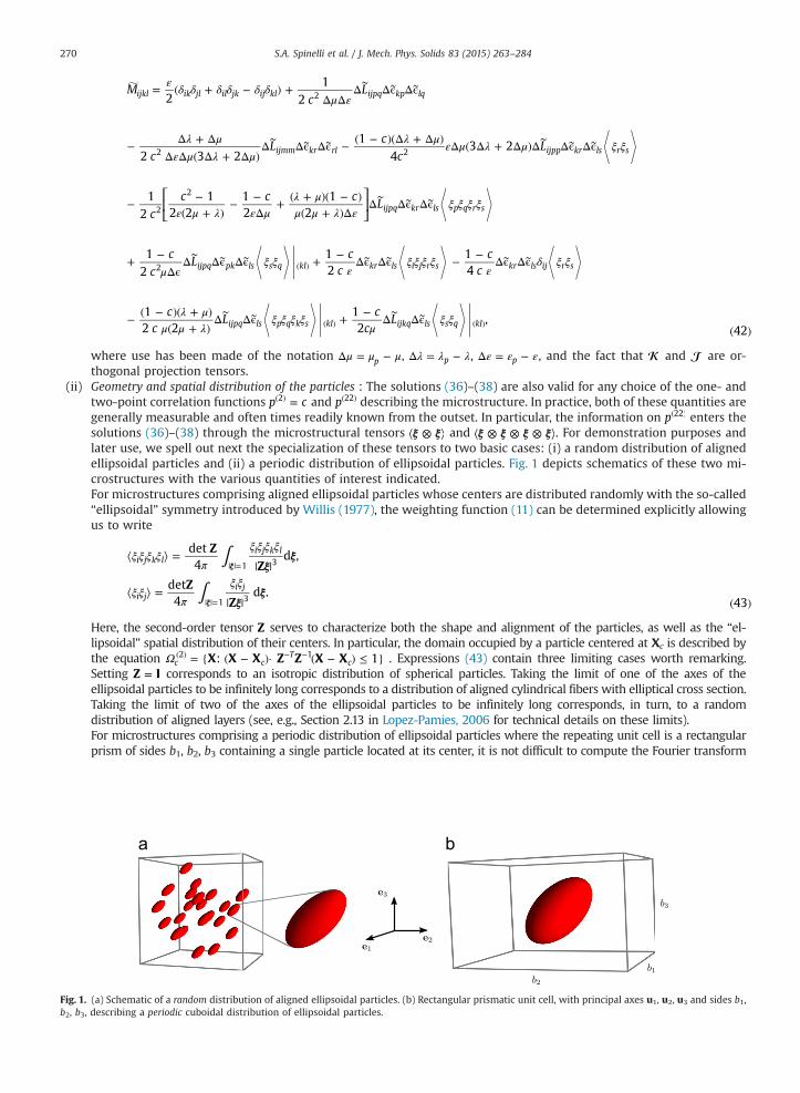
Fig. 1.b2, b3,

S.A. Spinelli et al. / J. Mech. Phys. Solids 83 (2015) 263–284270

⎡⎣⎢

⎤⎦⎥

Mc

L

cL

cc

L

cc c c

L

cc

Lc

cc

c

cc

Lc

cL

21

2

2 3 21

43 2

12

12 2

12

12

12

12

14

12 2

12

,42

ijkl ik jl il jk ij kl ijpq kp lq

ijmm kr rl ijpp kr ls r s

ijpq kr ls p q r s

ijpq pk ls s q kl kr ls i j r s kr ls ij r s

ijpq ls p q k s kl ijkq ls s q kl

2

2 2

2

2

2

ε δ δ δ δ δ δμ ε

λ με μ λ μ

λ μ ε μ λ μ ξ ξ

ε μ λ ε μλ μμ μ λ ε

ξ ξ ξ ξ

μξ ξ

εξ ξ ξ ξ

εδ ξ ξ

λ μμ μ λ

ξ ξ ξ ξμ

ξ ξ

= ( + − ) +Δ Δ

Δ Δϵ Δϵ

− Δ + ΔΔ Δ ( Δ + Δ )

Δ Δϵ Δϵ − ( − )(Δ + Δ ) Δ ( Δ + Δ )Δ Δϵ Δϵ

− −( + )

− −Δ

+ ( + )( − )( + )Δ

Δ Δϵ Δϵ

+ −Δϵ

Δ Δϵ Δϵ + − Δϵ Δϵ − − Δϵ Δϵ

− ( − )( + )( + )

Δ Δϵ + − Δ Δϵ( )

∼ ∼

∼ ∼ ∼ ∼

∼ ∼

∼ ∼ ∼ ∼ ∼ ∼

∼ ∼

∼

∼ ∼

∼

∼

∼ ∼

( )

( ) ( )

where use has been made of the notation pμ μ μΔ = − , pλ λ λΔ = − , pε ε εΔ = − , and the fact that and are or-thogonal projection tensors.

(ii)

Geometry and spatial distribution of the particles : The solutions (36)–(38) are also valid for any choice of the one- andtwo-point correlation functions p c2 =( ) and p 22( ) describing the microstructure. In practice, both of these quantities aregenerally measurable and often times readily known from the outset. In particular, the information on p 22( ) enters thesolutions (36)–(38) through the microstructural tensors ξ ξ⟨ ⊗ ⟩ and ξ ξ ξ ξ⟨ ⊗ ⊗ ⊗ ⟩. For demonstration purposes andlater use, we spell out next the specialization of these tensors to two basic cases: (i) a random distribution of alignedellipsoidal particles and (ii) a periodic distribution of ellipsoidal particles. Fig. 1 depicts schematics of these two mi-crostructures with the various quantities of interest indicated.For microstructures comprising aligned ellipsoidal particles whose centers are distributed randomly with the so-called“ellipsoidal” symmetry introduced by Willis (1977), the weighting function (11) can be determined explicitly allowingus to write

ZZ

ZZ

det4

d ,

det4

d .43

i j k li j k l

i ji j

1 3

1 3

∫

∫ξ

ξ

ξξ

ξ ξ ξ ξπ

ξ ξ ξ ξ

ξ ξπ

ξ ξ

⟨ ⟩ =| |

⟨ ⟩ =| | ( )

ξ

ξ

| |=

| |=

Here, the second-order tensor Z serves to characterize both the shape and alignment of the particles, as well as the “el-lipsoidal” spatial distribution of their centers. In particular, the domain occupied by a particle centered at Xc is described bythe equation X X X:c c

2Ω = { ( − )·( ) Z Z X X 1Tc

1( − ) ≤ }− − . Expressions (43) contain three limiting cases worth remarking.Setting Z I= corresponds to an isotropic distribution of spherical particles. Taking the limit of one of the axes of theellipsoidal particles to be infinitely long corresponds to a distribution of aligned cylindrical fibers with elliptical cross section.Taking the limit of two of the axes of the ellipsoidal particles to be infinitely long corresponds, in turn, to a randomdistribution of aligned layers (see, e.g., Section 2.13 in Lopez-Pamies, 2006 for technical details on these limits).For microstructures comprising a periodic distribution of ellipsoidal particles where the repeating unit cell is a rectangularprism of sides b1, b2, b3 containing a single particle located at its center, it is not difficult to compute the Fourier transform

(a) Schematic of a random distribution of aligned ellipsoidal particles. (b) Rectangular prismatic unit cell, with principal axes u1, u2, u3 and sides b1,describing a periodic cuboidal distribution of ellipsoidal particles.

S.A. Spinelli et al. / J. Mech. Phys. Solids 83 (2015) 263–284 271

(13)2 of its two-point correlation function and reciprocal lattice (14)–(15) in order to deduce that

cc

cc

Z Z Z

Z

Z Z Z

Z

1

9 sin cos,

1

9 sin cos.

44

i j k li j k l

i ji j

p p pp p p 0

2

4 6

p p pp p p 0

2

2 6

1 2 31 2 3

1 2 31 2 3

∑ ∑ ∑

∑ ∑ ∑

ξ ξ ξ

ξ ξ

ξ ξ ξ

ξ ξ

ξ ξ ξ ξξ ξ ξ ξ

ξ ξξ ξ

⟨ ⟩ =−

( | | − | | | |)| | | |

⟨ ⟩ =−

( | | − | | | |)| | | |

( )

{ }

{ }

=−∞

∞

=−∞

∞

=−∞

∞

− = = =

=−∞

∞

=−∞

∞

=−∞

∞

− = = =

In these expressions, Z describes, as in the foregoing, the shape and alignment of the particles, c b b bZ4 det /3 1 2 3π= ,and

b b bu u u

2p

2p

2p

4511 1

22 2

33 3ξ π π π= + +

( )

in terms of the summation integers p , p , p1 2 3, where the mutually orthogonal unit vectors u1, u2, u3 stand for theprincipal axes of the unit cell, as depicted in Fig. 1(b). Setting Z I= in (44) corresponds to a periodic distribution ofspherical particles. The limiting cases of a periodic distribution of aligned cylindrical fibers with elliptical cross sectionand a periodic distribution of aligned layers are also contained in expressions (44).

(iii)

Connection with the Hashin-Shtrikman variational principles in elastostatics and electrostatics : By construction, theunderlying microstructure associated with the solutions (36)–(38) corresponds to a distribution of disconnectedparticles that interact in such a manner that their deformation gradient and electric field — irrespectively of the valueof the volume fraction of particles c — are uniform and the same in each particle (see Appendix B in Lopez-Pamies,2014).An interesting implication of such a special type of intra-particle fields is that the solutions (36) and (37), respectively,for the effective modulus of elasticity L

∼and effective permittivity ϵ∼ agree identically with the variational approx-

imations obtained from the Hashin–Shtrikman variational principles in elastostatics (Hashin and Shtrikman, 1962a)and electrostatics (Hashin and Shtrikman, 1962b) when choosing the reference medium to coincide with the matrixmaterial and the trial polarization field to be constant per phase (so that the fields within the particles are alsoconstant). A corollary of this agreement is that the solutions (36) and (37) coincide identically with one of the Hashin–Shtrikman bounds when the elastic and dielectric properties of the matrix and particles are well ordered: the result(36) agrees with the upper (lower) bound in elastostatics when L L2 1<( ) ( ) (L L2 1>( ) ( )) in the sense of quadratic forms,while the result (37) agrees with the upper (lower) bound in electrostatics when 2 1ϵ ϵ<( ) ( ) ( 2 1ϵ ϵ>( ) ( )) also in the senseof quadratic forms. In view of these connections, it would be interesting to explore in future studies whether thesolution (38) for the effective electrostrictive tensor M possesses similar extremal properties.

(iv)

Connection with the classical results for dilute suspensions of ellipsoidal particles in elastostatics and electrostatics : Afurther implication of the uniformity of the intra-particle fields is that the solutions (36) and (37) agree with theclassical results for the effective modulus of elasticity L

∼(Eshelby, 1957) and effective permittivity ϵ∼ (see, e.g., Bergman,

1978 and references therein) of a dilute suspension of aligned ellipsoidal particles. By contrast, through a comparisonwith an exact solution available for spherical particles, we show in the next section that expression (38) does notcoincide in general with the effective electrostrictive tensor M of a dilute suspension of aligned ellipsoidal particles.

5. Sample results for dielectric elastomers filled with spherical particles

In addition to their theoretical value in providing a rigorous analytical solution for the electromechanical response ofdielectric elastomers with general particulate microstructures, the results (36)–(38) provide a formidable tool to gain insightinto how the addition of particles may enhance the electromechanical properties of dielectric elastomers. In this section, weexamine the specialization of the results (36)–(38) to the basic case of dielectric elastomers filled with an isotropic dis-tribution of spherical particles with isotropic elastic dielectric properties. To gain further insight, we compare such resultswith an exact solution (Lefèvre and Lopez-Pamies, 2014) available for a random isotropic suspension of polydispersespherical particles as well as with new full-field solutions — constructed by means of the finite-element (FE) method — for arandom isotropic suspension of monodisperse spherical particles. In order to avoid loss of continuity, the details of the FEcalculations are presented in Appendix A.

The practical motivation to consider isotropic distributions of spherical particles stems from recent experimental find-ings, including those of Zhang et al. (2002), Huang and Zhang (2004), Huang et al. (2005), Carpi and de Rossi (2005), McCarthy et al. (2009), and Liu et al. (2013), which have shown that the addition of random distributions of roughly sphericalparticles, made up of high-permittivity or (semi-)conducting solids, into dielectric elastomers leads to a drastic enhance-ment of the electrostrictive capabilities of these materials. In the sequel, we deploy the theoretical results (36)–(38) toscrutinize such findings. Furthermore, we seek to identify what other type of fillers not yet utilized in experimental studies,such as liquid-like particles with high-permittivity and vacuous pores, may potentially lead to the enhancement of the

S.A. Spinelli et al. / J. Mech. Phys. Solids 83 (2015) 263–284272

overall elastic dielectric properties of dielectric elastomers.

5.1. The case of isotropic distributions of spherical particles with isotropic elastic dielectric properties

For the case of spherical particles whose centers are distributed with isotropic symmetry Z I= and the microstructuraltensors (43) reduce to

13

and1

15.

46i j ij i j k l ij kl ik jl il jkξ ξ δ ξ ξ ξ ξ δ δ δ δ δ δ= = ( + + )( )

For this class of microstructures, assuming, for definiteness, that the particles are made up of an isotropic elastic di-electric material with modulus of elasticity, permittivity, and electrostrictive tensor of the form (39), the solutions (36)–(38)specialize to

m mL I M2 3 , , , 47K Jϵμ κ ε= + = = + ( )∼ ∼∼∼ ∼

where it is recalled that the orthogonal projections tensor and are given by expressions (27), and

⎡

⎣⎢⎢

⎤

⎦⎥⎥

c

c c c

c

c

c

c c

mc

c

c c c

c

c c

c

cc

mc c c c

c c c

c c c c c c

c c c

5 3 4

6 9 4 3 2 6 1 2,

3 4

3 4 3,

3

2 1,

115

115

3 1 5 1 3

3 4

14 1

3 1 25 3 4

,

2

3 1 3 3 3 2 4

2 2 1 3 3 4

3 3 4 6 3 4 1 4 2

2 2 1 3 3 4 48

p

p

p

p p

p

p

Kp

p p

p

Jp p p

p p p

p p

p p p

22 2

2

2

2

2

μ μκ μ μ μ μ

κ μ μ κ μ μ

κ κκ μ κ κ

κ μ κ κ

ε εε ε ε

ε ε

εε

εε ε

μ ε ε εκ

εμ κ μ

ε ε

ε μ με μ

κ μμ κ μ

ε μ

ε εε ε ε κ κ μ

ε ε κ κ κ μ

ε ε ε κ κ μ

ε ε κ κ κ μ

= +( + )( − )

[( + ) + ( + ) ] + ( − )( + )

= +( + )( − )+ − ( − )

= +( − )

( + ) + ( − )

= + − Δ +( − )

( − )[ (( − ) + ( + ) ) + ]

( + )+

( + ) + ( − )

( − )Δ Δ

+ ( − )( + )( + )

Δ Δ

= − +( − ) ( − )[ ( + ) − ( + ) + ]

[( + ) + ( − ) ] ( ( − ) + + )

+( − )[ (( − ) + ) − ( − )( − ) + ( + ) ]

[( + ) + ( − ) ] ( ( − ) + + ) ( )

∼

∼ ∼

∼

∼

∼

∼

∼

with 2 /3κ λ μ= + , 2 /3p p pκ λ μ= + , μ μ μΔ = −∼ ∼ , ε ε εΔ = −∼ ∼ . The overall electromechanical constitutive response (7)–(8) forthis type of isotropic dielectric elastomer composites read then simply as

⎡⎣⎢

⎤⎦⎥

⎡⎣⎢

⎤⎦⎥

m m

mm

S LH ME E

H E E

H H H I H I E E E E I E E I

2 3

23

tr tr13 3 49

K J

TK

J

μ κ

μ κ

= + ⊗= ( + ) + ( + ) ⊗

= + − ( ) + ( ) + ⊗ − ( · ) + ( · )( )

∼

∼

∼

∼

∼

and

D E E 50ϵ ε= = ( )∼ ∼

to leading order in the limit of small deformations and moderate electric fields.The above results contain several limiting cases worth recording explicitly:

�

Dilute volume fraction of particles: In the fundamental limit when the particles are present in dilute volume fraction asc 0→ +, the effective electromechanical material parameters (48) reduce asymptotically to

S.A. Spinelli et al. / J. Mech. Phys. Solids 83 (2015) 263–284 273

c

c

c

m c

m c

5 3 4

9 8 6 2,

3 4

3 4,

3

2,

3 3 23 41 7 19 126 137 9 17

5 2 6 2 9 8,

2

3 9 6 4

2 2 3 4 51

p

p

p

p

p

p

Kp p p p p p

p p

Jp p

p p

2

μ μκ μ μ μ μ

κ μ μ κ μ μ

κ κκ μ κ κ

κ μ

ε εε ε εε ε

εε ε μ εκ εμ ε κ ε μ μ εκ εμ ε κ ε μ ε

ε ε μ κ μ μ κ μ

ε ε ε κ κ μ εε ε κ μ

= +( + )( − )

( + ) + ( + )

= +( + )( − )

+

= +( − )

+

= +( − )[ ( + + + ) + ( + + − )]

( + ) [ ( + ) + ( + )]

= − −( − )( − + )

( + )( + ) ( )

∼

∼

∼

up to O(c).

� Rigid particles with infinite permittivity: In the limit of rigid infinite-permittivity particles when ,p pμ κ =+∞ and pε =+∞,

the effective electromechanical material parameters (48) reduce to

cc

cc

cc

mc c c

cm

c cc

5 3 46 1 2

,3 4

3 1,

31

,

3 7 1 9 1910 1 2

,2

3 22 1

.52

K J2 2

μ μ κ μκ μ

μ κ κ κ μ ε ε ε

ε κ μκ μ

ε ε ε

= + ( + )( − )( + )

= + ( + )( − )

= +−

= + [ ( − ) − ( − ) ]( − ) ( + )

= − + ( + )( − ) ( )

∼∼∼

If, in addition, the underlying elastomeric matrix is incompressible (κ =+∞), these formulae reduce further to

cc

cc

mc

cm

c cc

52 1

, ,3

1,

2110 1

,2

3 22 1

.53K J 2

μ μ μ κ ε ε ε

ε ε ε ε

= +( − )

=+∞ = +−

= +( − )

= − + ( + )( − ) ( )

∼∼∼

The results (52)–(53) are relevant for dielectric elastomer composites wherein the filler particles are typical ceramics(e.g., titania) or metals (e.g., iron), which generally exhibit much larger stiffness and permittivity (infinitely larger forthe case of metals) than elastomers.

�

Liquid particles with infinite permittivity: The case 0pμ = , pκ =+∞, and pε =+∞ corresponds to particles that are liquid-like(incompressible with vanishingly small shear modulus) and of infinite permittivity. Granted these limiting values forthe properties of the particles, the effective electromechanical material parameters (48) reduce to

cc c

cc

cc

mc c c

c c cm

c cc

5 3 49 6 4 2 3

,3 4

3 1,

31

,

3 3 7 3 27 175 1 9 6 4 2 3

,2

3 22 1

.54K J 2

μ μ κ μκ μ

μ κ κ κ μ ε ε ε

ε κ μκ μ

ε ε ε

= − ( + )( + ) + ( + )

= + ( + )( − )

= +−

= + [ ( + ) + ( − ) ]( − )[( + ) + ( + ) ]

= − + ( + )( − ) ( )

∼∼∼

When the underlying elastomeric matrix is incompressible (κ =+∞), these formulae reduce further to

cc

cc

mc c

c cm

c cc

53 2

, ,3

1,

3 3 75 1 3 2

,2

3 22 1

.55K J 2

μ μ μ κ ε ε ε

ε ε ε ε

= −+

=+∞ = +−

= + ( + )( − )( + )

= − + ( + )( − ) ( )

∼∼∼

Compared with elastomers, many fluids (e.g., water) and eutectic alloys (e.g., Galinstan) can be idealized as in-compressible and as having zero shear modulus and infinite permittivity (see, e.g., Wang et al., 2012; Fassler and Majidi,2015). Expressions (54)–(55) are relevant for such type of filler particles.

�

Porous dielectric elastomers: The limiting values , 0p pμ κ = , p 0ε ε= , κ =+∞, where 0ε stands for the permittivity of vacuum,correspond to an incompressible matrix containing an isotropic distribution of vacuous pores. In this case, the effectiveelectromechanical material parameters (48) reduce to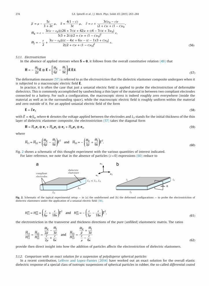

Fig.diele

S.A. Spinelli et al. / J. Mech. Phys. Solids 83 (2015) 263–284274

cc

cc

cc c

mc c c c c

c c c

mc c c c

c c

53 2

,4 1

3,

32 1

,

3 26 7 42 4 7 35 3 2 2 1

,

23 4 6 1 3

2 2 1.

56

K

J

0

0

0 0

02

0 0

02

μ μ μ κ μ ε εε ε ε

ε ε

εε ε ε ε

ε εε

ε ε ε ε εε ε

ε

= −+

= ( − ) = +( − )

( + ) + ( − )

= −( − )[(( + ) + ) + (( − ) + ) ]

( + )[( + ) + ( − ) ]

= − +( − )[(( − ) + ) − ( − )( + ) ]

[( + ) + ( − ) ] ( )

∼∼∼

5.1.1. ElectrostrictionIn the absence of applied stresses when S 0= , it follows from the overall constitutive relation (49) that

⎡⎣⎢

⎤⎦⎥

m m mH E E E E I

2 6 9.

57K K J

μ μ κ= − ⊗ + − ( · )

( )∼∼ ∼

The deformation measure (57) is referred to as the electrostriction that the dielectric elastomer composite undergoes when itis subjected to a macroscopic electric field E.

In practice, it is often the case that just a uniaxial electric field is applied to probe the electrostriction of deformabledielectrics. This is commonly accomplished by sandwiching a thin layer of the material in between two compliant electrodesconnected to a battery. For such a configuration, the macroscopic stress is indeed roughly zero everywhere (inside thematerial as well as in the surrounding space), while the macroscopic electric field is roughly uniform within the materialand zero outside of it. For an applied uniaxial electric field of the form

EE e 583= ( )

with E L/ 3= Φ , where Φ denotes the voltage applied between the electrodes and L3 stands for the initial thickness of the thinlayer of dielectric elastomer composite, the electrostriction (57) takes the diagonal form

H H HH e e e e e e , 5911 1 1 22 2 2 33 3 3= ⊗ + ⊗ + ⊗ ( )

where

⎛⎝⎜

⎞⎠⎟

⎛⎝⎜

⎞⎠⎟H H

m mE H

m mE

6 9and

3 9.

60K J K J

11 222

332

μ κ μ κ= = − = − +

( )∼ ∼∼ ∼

Fig. 2 shows a schematic of this thought experiment with the various quantities of interest indicated.For later reference, we note that in the absence of particles (c¼0) expressions (60) reduce to

2. Schematic of the typical experimental setup — in (a) the undeformed and (b) the deformed configurations — to probe the electrostriction ofctric elastomers under the application of a uniaxial electric field (58).

⎛⎝⎜

⎞⎠⎟

⎛⎝⎜

⎞⎠⎟H H E H E

6 18and

3 18,

61m m m11 22

233

2εμ

εκ

εμ

εκ

= = + = − −( )

the electrostriction in the transverse and thickness directions of the pure (unfilled) elastomeric matrix. The ratios

HH

HH

m m

HH

m m

2 3

2 6

and3

6 62m m

K J

m

K J

11

11

22

22

33

33

μ κεμ

εκ

μ κεμ

εκ

= =−

+=

+

−( )

∼ ∼∼ ∼

provide then direct insight into how the addition of particles affects the electrostriction of dielectric elastomers.

5.1.2. Comparison with an exact solution for a suspension of polydisperse spherical particlesIn a recent contribution, Lefèvre and Lopez-Pamies (2014) have worked out an exact solution for the overall elastic

dielectric response of a special class of isotropic suspensions of spherical particles in rubber, the so-called differential coated

S.A. Spinelli et al. / J. Mech. Phys. Solids 83 (2015) 263–284 275

sphere (DCS) assemblage (see, e.g., Avellaneda, 1987; Chapter 10.5 in Milton, 2002). Roughly speaking, this class of sus-pensions comprises spherical particles of infinitely many sizes distributed in such a way that particles of any given com-parable size are far apart from each other and surrounded by particles of much smaller size. For the case of interest here,when the elastomeric matrix material and the particles are characterized by relations (24) and (39), the effective shearmodulus, bulk modulus, permittivity, and electrostrictive coefficients of such suspensions read as

⎡⎣ ⎤⎦ ⎛⎝⎜

⎞⎠⎟

⎡⎣ ⎤⎦

⎡⎣⎤⎦

q q q q

q

c

c

c

c c

mA A c

c

B

c

B c c c c

c

B

c

c c

c

B c c c c c

c

mc c c c

c c c

c c c c c c

c c c

4

2,

3 4

3 4 3,

3

2 1,

2 75 55 21 3

5 15 1135

11

2 1 20 2 10 5

452

15 15 11

15 32 7 2 3 7 2 3

9 3 5 2 11 2

1 5 7 5 7 5

15,

2

3 1 3 3 3 2 4

2 2 1 3 3 4

3 3 4 6 3 4 1 4 2

2 2 1 3 3 4,

63

p

p p

p

p

Kp p p p p

p p p

p p

p p

p p p p

p p p p

p

p

Jp p p

p p p

p p

p p p

DCS 2 22

1 3

1

DCS

DCS

DCSDCS 2

1 32/3

22

8/3DCS 2

1DCS 2 2 2

2 23

DCS 2

2 2

2 2 2

5/3 2 2 2 2

4DCS 2

2

DCS2

2

2

( )( ) ( )

μ μ

κ κκ μ κ κ

κ μ κ κ

ε εε ε ε

ε ε

ε ε ε κ μ κ μ

ε ε κ μ εε ε

ε ε ε εε ε

ε ε εε ε

ε ε ε κ μ

ε ε κ μ ε ε ε ε κ μ ε ε κ μ

κ ε εε ε μ ε εε ε

ε ε ε κ μ κ ε κ μ

εμ ε ε

ε εε ε ε κ κ μ

ε ε κ κ κ μ

ε ε ε κ κ μ

ε ε κ κ κ μ

=+ +

= +( + )( − )+ − ( − )

= +( − )

( + ) + ( − )

=( − ) ( + ) + ( + )

( − ) ( + )− − ( − )

+( − )( − ) ( + ) − ( − ) + ( + )

( − )−

( − )( − ) ( + )

× ( − ) ( + ) + ( + )( − )( + ) − ( + ) ( + )

+ + + + − + −

+( − )( − ) [ ( + ( − ) + ) − (( + ) + ( + ) )]

( − )

= − +( − ) ( − )[ ( + ) − ( + ) + ]

[( + ) + ( − ) ] ( ( − ) + + )

+( − )[ (( − ) + ) − ( − )( − ) + ( + ) ]

[( + ) + ( − ) ] ( ( − ) + + ) ( )

∼

∼∼

∼ ∼

∼

∼

∼

where the two sets of parameters q1, q2, q3 and A1, A3, B1, B2, B3, B4 are defined, respectively, in Appendices II and I in Lefèvreand Lopez-Pamies (2014).

Remarkably, the results (48)2, (48)3, and (48)5 for the effective bulk modulus κ∼, effective permittivity ε∼, and effectiveelectrostrictive coefficient mJ are seen to agree identically with the corresponding effective material parameters (63)2, (63)3,and (63)5 for a suspension of polydisperse spherical particles. By contrast, the results (48)1 and (48)4 for the effective shearmodulus μ∼ and effective electrostrictive coefficient mK differ in general from expressions (63)1 and (63)4. In the dilute limitof particles as c 0→ +, these latter expressions reduce asymptotically to

c

m c

5 3 4

9 8 6 2,

3 6 2 2 27 28 4

2 6 2 9 8 64

p

p

Kp p p p

p p

DCS

DCS2

μ μκ μ μ μ μ

κ μ μ κ μ μ

εε ε μ ε ε κ μ μ εκ εμ ε μ ε

ε ε μ κ μ μ κ μ

= +( + )( − )

( + ) + ( + )

= +( − )[ ( + )( + ) + ( + − )]

( + ) [ ( + ) + ( + )] ( )

∼

up to O(c). Thus, as anticipated in remark iv of Section 4, the result (48)1 does agree identically with the exact effective shearmodulus (64)1 for a dilute suspension of spherical particles (cf . expression (51)1), but the same is not true for the result(48)4, whose asymptotic form (51)4 in the dilute limit is in general different from the effective electrostrictive coefficient(64)2 .

The above comparison reveals that the effective electromechanical material parameters (48), even though exact for adifferent class of two-phase particulate isotropic microstructures, serve as well to describe — approximately in general, butexactly in some special cases — the overall elastic dielectric response of a random isotropic suspension of polydispersespherical particles. In this regard, we emphasize again that the microstructure for which the effective constants (48) areexact was selected to have the same one- and two-point correlation functions as an isotropic suspension of sphericalparticles; see remark ii of Section 4. In the sequel, we present further comparisons between the theoretical results (48) andfull-field simulations for a random isotropic suspension of monodisperse spherical particles.

5.2. Results for stiff particles with high permittivity

We begin by examining the case of dielectric elastomer composites wherein the filler particles are mechanically stifferthan the elastomeric matrix and also exhibit higher permittivity. As pointed out above, this is the case that has hitherto

S.A. Spinelli et al. / J. Mech. Phys. Solids 83 (2015) 263–284276

received most attention by the experimental community, presumably because most filler materials with high permittivity or(semi-)conducting behavior (e.g., ceramics, metals) are stiffer than elastomers.

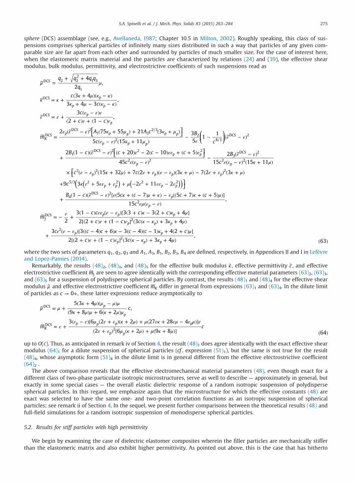
Fig. 3(a), (b), (c) show, respectively, results for the normalized effective shear modulus /μ μ∼ , permittivity /ε ε∼ , and elec-trostrictive coefficients m /K ε , �2m /J ε of a dielectric elastomer composite comprised of a nearly incompressible elastomericmatrix with / 103κ μ = and stiff high-permittivity filler particles with / 10p

5μ μ = , / 10p5κ μ = , and / 10p

2ε ε = , as functions of thevolume fraction of particles c (no results for the effective bulk modulus κ∼ are included since the overall response is nearlyincompressible in this case). The rationale behind this choice of material parameters is that they are typical of many of thedielectric elastomer composites studied experimentally, such as for instance those of Liu et al. (2013), where the elastomer issilicone rubber ( 0.22 MPaμ = , 1 GPaκ = , 3.2 0ε ε= ) and the particles are made out of titania ( 110 GPapμ = , 220 GPapκ = ,

114p 0ε ε= ). In these and subsequent figures, the solid lines are associated with the theoretical results (48), while the dashedlines and solid circles stand for corresponding results based on the analytical solution (63) for isotropic suspensions ofpolydisperse spherical particles and on FE simulations for isotropic suspensions of monodisperse spherical particles.

As discussed in Section 5.1.2, Fig. 3(a)–(c) illustrate that the theoretical results are in fairly good agreement with theresults for suspensions of polydisperse and also monodisperse spherical particles, save quantitatively for the effective shearmodulus μ∼ when c 0.15> and for the effective electrostrictive coefficient mK when c 0.05> . Another immediate observationfrom Fig. 3(a) and (b) is that the addition of stiff high-permittivity particles enhances both the stiffness and permittivity ofthe dielectric elastomer. Fig. 3(c) shows that this is also the case for the electrostrictive coefficients mK and mJ . According toEq. (57), and as expected on physical grounds, these trends set up a direct competition of effects for the overall

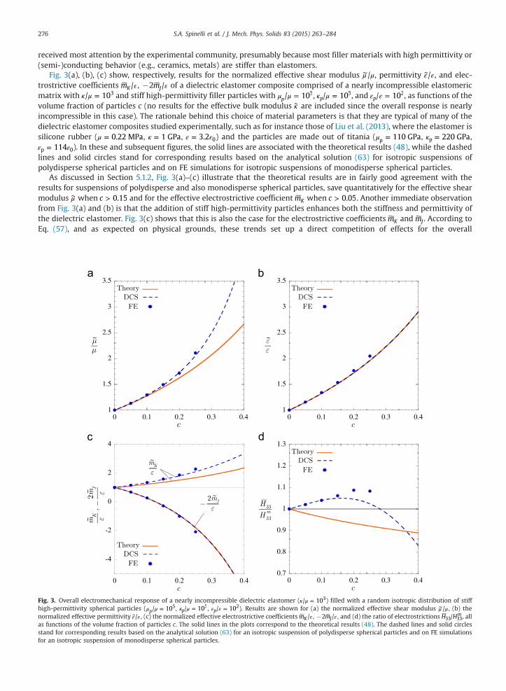
Fig. 3. Overall electromechanical response of a nearly incompressible dielectric elastomer ( / 103κ μ = ) filled with a random isotropic distribution of stiffhigh-permittivity spherical particles ( / 10p

5μ μ = , / 10p5κ μ = , / 10p

2ε ε = ). Results are shown for (a) the normalized effective shear modulus /μ μ∼ , (b) thenormalized effective permittivity /ε ε∼ , (c) the normalized effective electrostrictive coefficients m /K ε , �2m /J ε , and (d) the ratio of electrostrictions H H/ m

33 33, allas functions of the volume fraction of particles c. The solid lines in the plots correspond to the theoretical results (48). The dashed lines and solid circlesstand for corresponding results based on the analytical solution (63) for an isotropic suspension of polydisperse spherical particles and on FE simulationsfor an isotropic suspension of monodisperse spherical particles.

S.A. Spinelli et al. / J. Mech. Phys. Solids 83 (2015) 263–284 277

electrostriction capabilities of the composite. To see which enhancement proves dominant, if the enhancement in stiffness(which makes the material less deformable) or that in permittivity and electrostrictive coefficients (which makes thematerial more prone to deform under the application of an electric field), we turn to examine the behavior of the ratio ofelectrostrictions H H/ m

33 33 associated with the response of the composite under a uniaxial electric field; see Section 5.1.1.Fig. 3(d) shows plots of the ratio H H/ m

33 33 as a function of the volume fraction of particles c (no results for the ratio H H/ m11 11

are shown here since the overall near incompressibility of the composite implies that H H H H/ 1/2 /m m11 11 33 33≈ ). The theoretical

results indicate that H H/ 1m33 33 < , that is, the addition of particles leads to a reduction in electrostriction. Physically, this entails

that the enhancement in stiffness due to the addition of particles dominates over the enhancement in permittivity resultingin the filled elastomer undergoing less electrostriction than the unfilled elastomer when exposed to the same electric field.This behavior is in contrast to that displayed by the suspensions of spherical particles, which initially and up to about c¼0.3exhibit an enhancement in electrostriction (H H/ 1m

33 33 > ) before displaying a reduction (H H/ 1m33 33 < ).

While qualitatively different, all three sets of results in Fig. 3(d) agree in that the reduction or enhancement is quanti-tatively small, indeed H H0.8 / 1.15m

33 33< < for the entire range of particle volume fractions considered, c0 0.4≤ ≤ . Such adifference in qualitative behavior but agreement in quantitative behavior among three different exact results for threedifferent two-phase particulate isotropic microstructures suggests that the electrostriction capabilities of dielectric elas-tomers filled isotropically with stiff high-permittivity particles are highly sensitive to the details of the microstructure, butonly in a qualitative manner. Quantitatively, moreover, they suggest that the enhancement in stiffness provided by theaddition of filler particles essentially cancels out the enhancement in permittivity, so that there is ultimately little differencebetween the electrostriction capabilities of the unfilled and the filled elastomer (for particle volume fractions sufficientlyaway from percolation, of course).

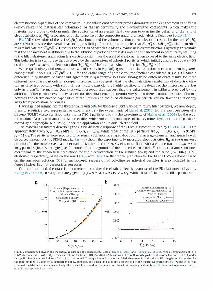
Having gained insight into the theoretical results (48) for the case of stiff high-permittivity filler particles, we now deploythem to scrutinize two representative experiments: (i) the experiments of Liu et al. (2013) for the electrostriction of asilicone (PDMS) elastomer filled with titania (TiO2) particles and (ii) the experiments of Huang et al. (2005) for the elec-trostriction of a polyurethane (PU) elastomer filled with semi-conductor copper phthalocyanine oligomer (o-CuPc) particles,coated by a polyacrylic acid (PAA), under the application of a uniaxial electric field.

The material parameters describing the elastic dielectric response of the PDMS elastomer utilized by Liu et al. (2013) areapproximately given by 0.22 MPaμ = , 1 GPaκ = , 3.2 0ε ε= , while those of the TiO2 particles are 110 GPapμ = , 220 GPapκ = ,

114p 0ε ε= . The particles were reported to be roughly spherical in shape, about 3 μm in average diameter, and spatially welldispersed throughout the PDMS matrix. Fig. 4(a) shows the experimentally measured electrostriction H11 in the transversedirection for the pure PDMS elastomer (solid triangles) and the PDMS elastomer filled with a volume fraction c¼0.082 ofTiO2 particles (hollow triangles), as functions of the magnitude of the applied electric field E . The dotted and solid linescorrespond to the theoretical predictions for the electrostriction of the unfilled (c¼0) and the filled (c¼0.082) PDMSelastomer, respectively, based on the result (60)1 with (48). The theoretical prediction for the filled PDMS elastomer basedon the analytical solution (63) for an isotropic suspension of polydisperse spherical particles is also included in thefigure (dashed line) for comparison purposes.

On the other hand, the material parameters describing the elastic dielectric response of the PU elastomer utilized byHuang et al. (2005) are approximately given by 9 MPaμ = , 5 GPaκ = , 8 0ε ε= , while those of the o-CuPc filler particles are

Fig. 4. Comparisons between the theoretical results and the experimental data of Liu et al. (2013) and Huang et al. (2005) for the electrostriction of (a) aPDMS elastomer filled with TiO2 particles at volume fraction c¼0.082 and (b) a PU elastomer filled with o-CuPc particles at volume fraction c¼0.073, underthe application of a uniaxial electric field with magnitude E . The experimental data for the filled elastomers is depicted as solid triangles, while the data forthe pure (unfilled) elastomers is depicted as hollow triangles. The dotted and solid lines correspond to the theoretical predictions (60) with (48) for thepure and the filled elastomers, respectively. The dashed lines stand for the predictions based on the analytical solution (63) for an isotropic suspension ofpolydisperse spherical particles.

S.A. Spinelli et al. / J. Mech. Phys. Solids 83 (2015) 263–284278

1 GPapμ = , 100 GPapκ = , 10p4

0ε ε= . In this case too, the particles were roughly spherical in shape, about 40 nm in diameter,and spatially well dispersed throughout the PU matrix. The volume fraction of the particles was reported to be approxi-mately c¼0.073. Fig. 4(b) shows the experimentally measured electrostriction H33 in the thickness direction for the pure PUelastomer (solid triangles) and the filled PU elastomer (hollow triangles), as functions of the magnitude of the appliedelectric field E . Similar to Fig. 4(a), the dotted and solid lines correspond to the theoretical predictions (60)2 with (48) for thepure (c¼0) and the filled (c¼0.073) PU elastomer, respectively, while the dashed line corresponds to the theoretical pre-diction for the filled PU elastomer based on the analytical solution (63).

It is apparent from Fig. 4(a) that the response of the filled PDMS elastomer exhibits a significant enhancement inelectrostriction, in the order of 50% increase, when compared with the pure PDMS elastomer. In disaccord with this ex-perimentally observed enhancement, as already discussed within the context of Fig. 3(d), the theoretical predictions showlittle change between the electrostriction of the pure and the filled PDMS elastomers. Fig. 4(b) shows an even more glaringdifference between the experimental response of the filled PU elastomer, which exhibits about a 20-fold enhancement inelectrostriction compared to the pure PU elastomer, and the theoretical predictions. This dramatic difference occurs con-sistently for the entire range of deformations H33 and electric fields E considered, including small values of H33 and E forwhich the asymptotic premise of “small” deformations and “moderate” electric fields — upon which the formulas (60) and(48) are based — is expected to be applicable.

We conjecture that the drastic electrostriction enhancement observed in the experiments may be due to the presence ofhigh-permittivity interphases and/or interphasial free charges around the filler particles, which the proposed theory doesnot account for. Indeed, it is well known that in elastomers filled with stiff particles the “anchoring” of the polymeric chainsof the matrix onto the particles forces the chains into conformations that are very different from those in the bulk, henceresulting in “interphases” of possibly several tens of nanometers in thickness that have very different mechanical andphysical properties from those in the bulk (see, e.g., Lewis, 2004; Roy et al., 2005; Goudarzi et al., 2015 and referencestherein). Furthermore, free charges in such interphases may be present from the outset because of the fabrication process ofthe specimens. They may also be injected from the particles upon the application of an electric field. In this regard, we notethat in the experiments of Huang et al. (2005) the particles were made out of an organic semi-conductor coated by ananionic polyacrylic acid. Whatever their origin, the presence of interphasial charges has been recently shown to have thepotential to lead to extreme enhancements of the overall dielectric response of particulate composites and, by the sametoken, extreme enhancements of their electrostrictive response (Lopez-Pamies et al., 2014).

5.3. Results for liquid-like particles with high permittivity

Next, we examine the case of dielectric elastomer composites wherein the filler particles are liquid-like, in the sense thatthey are characterized by nearly incompressible behavior and vanishingly small shear stiffness, and exhibit a higher per-mittivity than the elastomeric matrix. Such properties are distinctive of many common fluids such as water and specialtypes of alloys such as Galistan. The practical interest in this type of dielectric elastomer composites is that increasing thecontent of their fillers increases the overall permittivity at the same time that it also increases the overall deformability (incontrast to the mechanically stiff particles considered in the preceding subsection) and thus has the potential to bestow theresulting composites with exceptionally enhanced electrostriction capabilities.

Fig. 5(a), (b), (c) show, respectively, results for the normalized effective shear modulus /μ μ∼ , permittivity /ε ε∼ , and electro-strictive coefficients m /K ε , �2m /J ε of a dielectric elastomer composite comprised of a nearly incompressible elastomeric matrixwith / 103κ μ = and liquid-like high-permittivity filler particles with / 10p

2μ μ = − , / 10p3κ μ = , and / 10p

2ε ε = , as functions of thevolume fraction of particles c. Fig. 5(d) shows the associated ratio of electrostrictions H H/ m

33 33 also as a function of c.Consistent with the preceding case for mechanically stiff particles, the theoretical results (48) are seen to be in fairly good

agreement with the results for suspensions of polydisperse and monodisperse spherical particles, save quantitatively for theeffective electrostrictive coefficient mK . As expected on physical grounds, Fig. 5(a) and (b) confirms that the addition ofliquid-like high-permittivity particles decreases the overall shear stiffness but increases the overall permittivity of thecomposite. Fig. 5(c) shows that the effective electrostrictive coefficients mK and mJ increase also with the addition of suchfillers. This monotonic decrease in stiffness together with the increase in permittivity and electrostrictive coefficients entailthat the electrostriction capabilities of the resulting dielectric elastomer composite are enhanced with the addition of fillers.This is precisely what is shown in Fig. 5(d), which illustrates not only that indeed H H/ 1m

33 33 > for all c but also reveals thatmore than a 50% enhancement in electrostriction can be achieved with the addition of a moderate content of liquid-likehigh-permittivity particles. It would be interesting to explore these encouraging findings experimentally.

5.4. Results for porous dielectric elastomers

Finally, we consider the overall electromechanical response of porous dielectric elastomers made up of a dielectricelastomer containing a random isotropic distribution of vacuous spherical pores. Here, it is important to recognize thatvacuous pores are mechanically softer at the same time that they exhibit lower permittivity than elastomers. Thus theiraddition results in an increase in overall deformability but also a decrease in overall permittivity setting up — similar to thecase of stiff high-permittivity fillers — a direct competition of effects for the overall electrostriction capabilities of thecomposite.

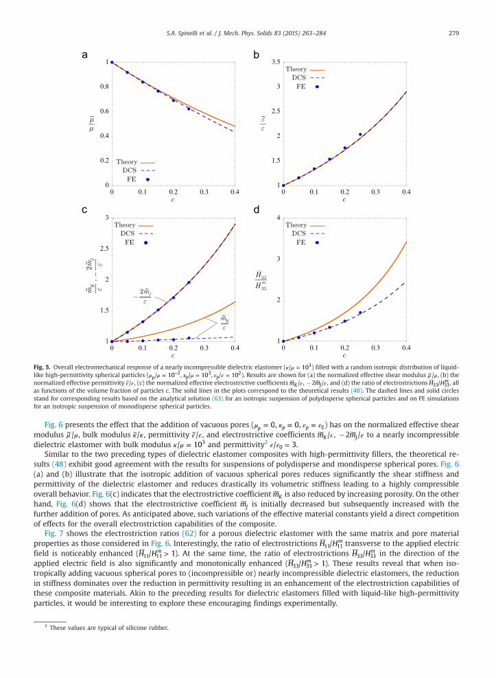
Fig. 5. Overall electromechanical response of a nearly incompressible dielectric elastomer ( / 103κ μ = ) filled with a random isotropic distribution of liquid-like high-permittivity spherical particles ( / 10p

2μ μ = − , / 10p3κ μ = , / 10p

2ε ε = ). Results are shown for (a) the normalized effective shear modulus /μ μ∼ , (b) thenormalized effective permittivity /ε ε∼ , (c) the normalized effective electrostrictive coefficients m /K ε , �2m /J ε , and (d) the ratio of electrostrictions H H/ m

33 33, allas functions of the volume fraction of particles c. The solid lines in the plots correspond to the theoretical results (48). The dashed lines and solid circlesstand for corresponding results based on the analytical solution (63) for an isotropic suspension of polydisperse spherical particles and on FE simulationsfor an isotropic suspension of monodisperse spherical particles.

S.A. Spinelli et al. / J. Mech. Phys. Solids 83 (2015) 263–284 279

Fig. 6 presents the effect that the addition of vacuous pores ( 0pμ = , 0pκ = , p 0ε ε= ) has on the normalized effective shearmodulus /μ μ∼ , bulk modulus /κ κ∼ , permittivity /ε ε∼ , and electrostrictive coefficients m /K ε , �2m /J ε to a nearly incompressibledielectric elastomer with bulk modulus / 103κ μ = and permittivity2 / 30ε ε = .

Similar to the two preceding types of dielectric elastomer composites with high-permittivity fillers, the theoretical re-sults (48) exhibit good agreement with the results for suspensions of polydisperse and mondisperse spherical pores. Fig. 6(a) and (b) illustrate that the isotropic addition of vacuous spherical pores reduces significantly the shear stiffness andpermittivity of the dielectric elastomer and reduces drastically its volumetric stiffness leading to a highly compressibleoverall behavior. Fig. 6(c) indicates that the electrostrictive coefficient mK is also reduced by increasing porosity. On the otherhand, Fig. 6(d) shows that the electrostrictive coefficient mJ is initially decreased but subsequently increased with thefurther addition of pores. As anticipated above, such variations of the effective material constants yield a direct competitionof effects for the overall electrostriction capabilities of the composite.

Fig. 7 shows the electrostriction ratios (62) for a porous dielectric elastomer with the same matrix and pore materialproperties as those considered in Fig. 6. Interestingly, the ratio of electrostrictions H H/ m

11 11 transverse to the applied electricfield is noticeably enhanced (H H/ 1m

11 11 > ). At the same time, the ratio of electrostrictions H H/ m33 33 in the direction of the

applied electric field is also significantly and monotonically enhanced (H H/ 1m33 33 > ). These results reveal that when iso-

tropically adding vacuous spherical pores to (incompressible or) nearly incompressible dielectric elastomers, the reductionin stiffness dominates over the reduction in permittivity resulting in an enhancement of the electrostriction capabilities ofthese composite materials. Akin to the preceding results for dielectric elastomers filled with liquid-like high-permittivityparticles, it would be interesting to explore these encouraging findings experimentally.

2 These values are typical of silicone rubber.

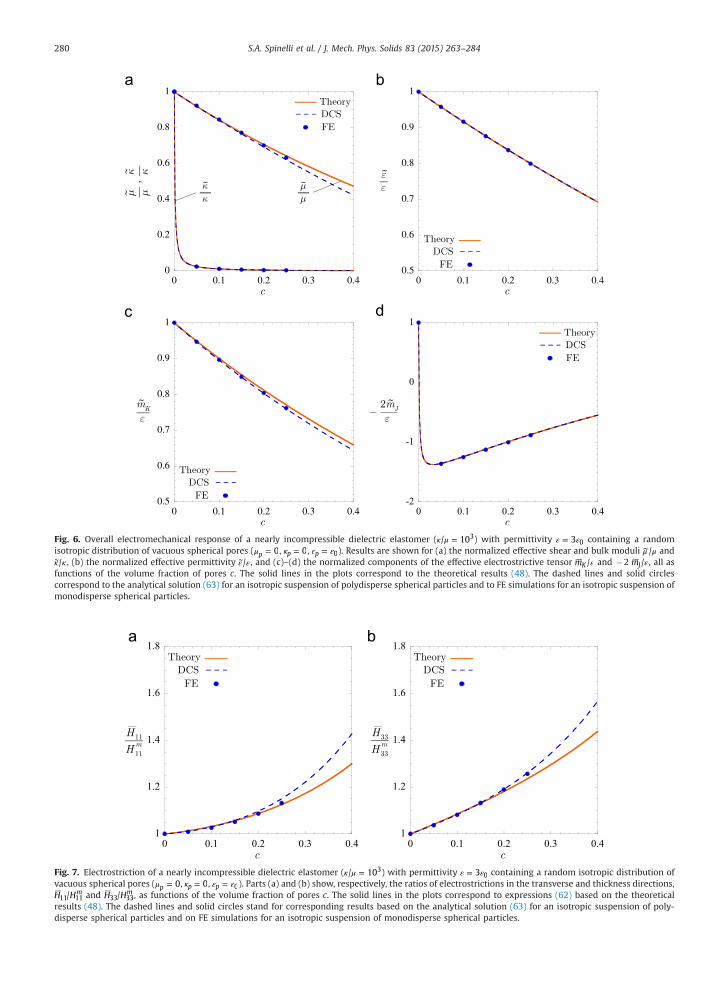
Fig. 6. Overall electromechanical response of a nearly incompressible dielectric elastomer ( / 103κ μ = ) with permittivity 3 0ε ε= containing a randomisotropic distribution of vacuous spherical pores ( 0pμ = , 0pκ = , p 0ε ε= ). Results are shown for (a) the normalized effective shear and bulk moduli /μ μ∼ and

/κ κ∼ , (b) the normalized effective permittivity /ε ε∼ , and (c)–(d) the normalized components of the effective electrostrictive tensor m /K ε and �2 m /J ε , all asfunctions of the volume fraction of pores c. The solid lines in the plots correspond to the theoretical results (48). The dashed lines and solid circlescorrespond to the analytical solution (63) for an isotropic suspension of polydisperse spherical particles and to FE simulations for an isotropic suspension ofmonodisperse spherical particles.

Fig. 7. Electrostriction of a nearly incompressible dielectric elastomer ( / 103κ μ = ) with permittivity 3 0ε ε= containing a random isotropic distribution ofvacuous spherical pores ( 0pμ = , 0pκ = , p 0ε ε= ). Parts (a) and (b) show, respectively, the ratios of electrostrictions in the transverse and thickness directions,H H/ m

11 11 and H H/ m33 33, as functions of the volume fraction of pores c. The solid lines in the plots correspond to expressions (62) based on the theoretical

results (48). The dashed lines and solid circles stand for corresponding results based on the analytical solution (63) for an isotropic suspension of poly-disperse spherical particles and on FE simulations for an isotropic suspension of monodisperse spherical particles.

S.A. Spinelli et al. / J. Mech. Phys. Solids 83 (2015) 263–284280

S.A. Spinelli et al. / J. Mech. Phys. Solids 83 (2015) 263–284 281

In summary, the above sample results have illustrated the capabilities of the general solutions (36)–(38) to provide quan-titative insight into the overall electromechanical response of dielectric elastomer composites. They have also served to revealthat for the case of dielectric elastomers filled with a random isotropic distribution of stiff, high-permittivity or (semi-)con-ducting, roughly spherical particles — the case that has hitherto received most attention by the experimental community —

interphasial phenomena may be crucial in understanding and exploiting the enhanced electrostriction that this promising classof materials is able to achieve. Furthermore, they have revealed that the study of dielectric elastomers filled with liquid-likehigh-permittivity or (semi-)conducting particles as well as porous dielectric elastomers may be worth pursuing.

Acknowledgments

Support for this work by the National Science Foundation through CAREER Grant CMMI–1219336 is gratefullyacknowledged.

Appendix A. FE calculations of the homogenized response of dielectric elastomer composites

In this appendix, we summarize the computation of the finite-element (FE) results presented in Section 5 for dielectricelastomers filled with an isotropic distribution of spherical particles.

Within the classical context of small deformations and moderate electric fields described in Section 1.1, the effectiveelectromechanical tensors L

∼, ϵ∼, M for a composite material with arbitrarily heterogeneous local modulus of elasticity

L L X= ( ), permittivity Xϵ ϵ= ( ), and electrostrictive tensor M M X= ( ) are given by the formulas

L L X1

d , 65ijkl ijmn mkl n,∫ΩΓ=

| | ( )∼

Ω

X1

d , 66ij im m j,∫Ωγϵ =

| |ϵ ( )

∼Ω

M M X1

d . 67ijkl mij n mnpq p k q l, , ,∫ΩΓ γ γ=

| | ( )Ω

Here, it is recalled that Ω stands for the domain occupied by the composite in its undeformed stress-free configuration andthe tensor fields Γ and γ are defined implicitly as the solutions to the following linear uncoupled boundary value problems:

L XX X0, with , , 68ijmn mkl n j ikl ik jl j, ,Γ Ω Γ δ δ Ω[ ] = ∈ = ∈ ∂ ( )

XX X0, with , . 69im m j i i ij j, ,γ Ω γ δ Ω[ϵ ] = ∈ = ∈ ∂ ( )

In the above expressions, the notation , j represents the partial differentiation with respect to the material point coordinate Xj

and Ω∂ stands for the boundary of the domain Ω.While the formulation (65)–(69) is formal in general, Tian (2007) and Tian et al. (2012) have shown it to be rigorous in

the context of composite materials with periodic microstructure. When the repeating unit cell Q chosen to describe such aperiodic microstructure is the unit cube Q X iX: 0, 1 1, 2, 3i= { ∈ [ ] = }, the general formulation (65)–(69) specializes to

L L Xd ,70ijkl

Qijmn mkl n,∫ Γ=

( )∼

Xd ,71ij

Qim m j,∫ γϵ = ϵ

( )∼

M M Xd ,72ijkl

Qmij n mnpq p k q l, , ,∫ Γ γ γ=

( )

where now the tensor fields Γ and γ are defined by

⎧⎨⎪

⎩⎪L Q

X X X X

X X X X

X X X X

QX X0, with

1, , 0, ,

, 1, , 0, ,

, , 1 , , 0 73

ijmn mkl n j

ikl ikl ik l

ikl ikl ik l

ikl ikl ik l

, ,

2 3 2 3 1

1 3 1 3 2

1 2 1 2 3

ΓΓ Γ δ δΓ Γ δ δΓ Γ δ δ

[ ] = ∈( ) − ( ) =( ) − ( ) =( ) − ( ) =

∈ ∂

( )

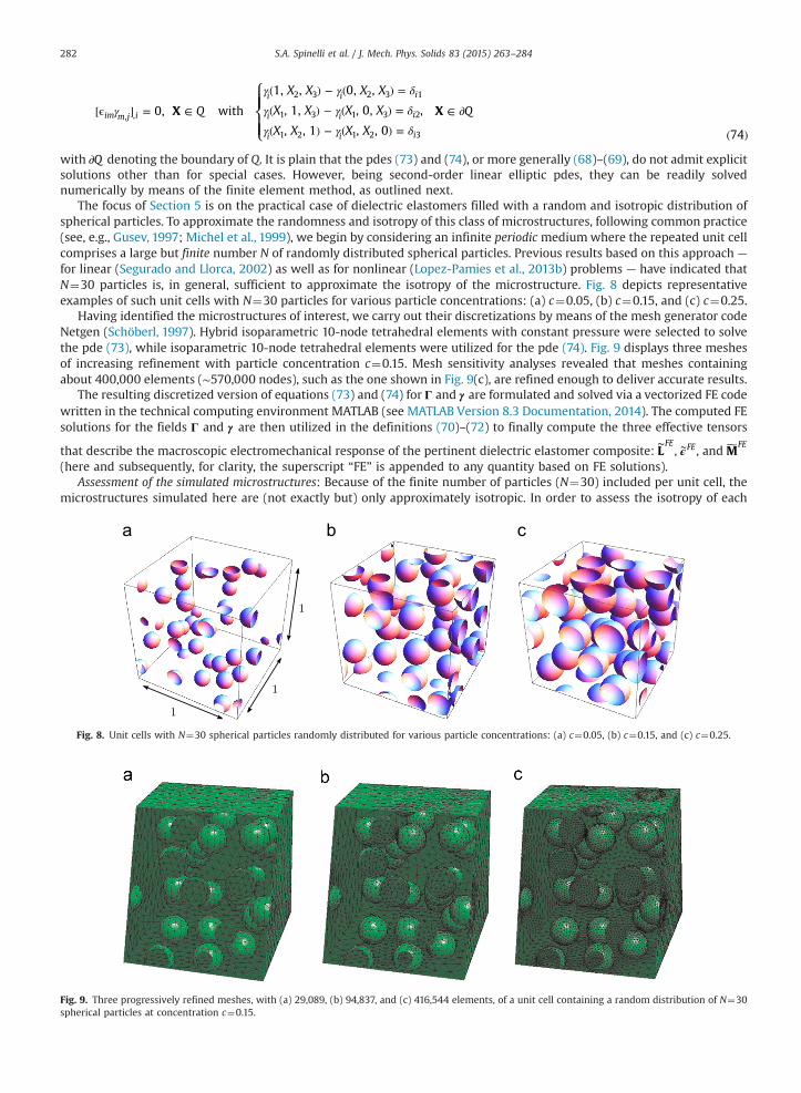
S.A. Spinelli et al. / J. Mech. Phys. Solids 83 (2015) 263–284282

⎧⎨⎪⎪

⎩⎪⎪

Q

X X X X

X X X X

X X X X

QX X0, with

1, , 0, ,

, 1, , 0, ,

, , 1 , , 0 74

im m j i

i i i

i i i

i i i

, ,

2 3 2 3 1

1 3 1 3 2

1 2 1 2 3

γ

γ γ δ

γ γ δ

γ γ δ

[ϵ ] = ∈

( ) − ( ) =

( ) − ( ) =

( ) − ( ) =∈ ∂

( )

with Q∂ denoting the boundary of Q. It is plain that the pdes (73) and (74), or more generally (68)–(69), do not admit explicitsolutions other than for special cases. However, being second-order linear elliptic pdes, they can be readily solvednumerically by means of the finite element method, as outlined next.

The focus of Section 5 is on the practical case of dielectric elastomers filled with a random and isotropic distribution ofspherical particles. To approximate the randomness and isotropy of this class of microstructures, following common practice(see, e.g., Gusev, 1997; Michel et al., 1999), we begin by considering an infinite periodic mediumwhere the repeated unit cellcomprises a large but finite number N of randomly distributed spherical particles. Previous results based on this approach —

for linear (Segurado and Llorca, 2002) as well as for nonlinear (Lopez-Pamies et al., 2013b) problems — have indicated thatN¼30 particles is, in general, sufficient to approximate the isotropy of the microstructure. Fig. 8 depicts representativeexamples of such unit cells with N¼30 particles for various particle concentrations: (a) c¼0.05, (b) c¼0.15, and (c) c¼0.25.

Having identified the microstructures of interest, we carry out their discretizations by means of the mesh generator codeNetgen (Schöberl, 1997). Hybrid isoparametric 10-node tetrahedral elements with constant pressure were selected to solvethe pde (73), while isoparametric 10-node tetrahedral elements were utilized for the pde (74). Fig. 9 displays three meshesof increasing refinement with particle concentration c¼0.15. Mesh sensitivity analyses revealed that meshes containingabout 400,000 elements (∼570,000 nodes), such as the one shown in Fig. 9(c), are refined enough to deliver accurate results.

The resulting discretized version of equations (73) and (74) for Γ and γ are formulated and solved via a vectorized FE codewritten in the technical computing environment MATLAB (see MATLAB Version 8.3 Documentation, 2014). The computed FEsolutions for the fields Γ and γ are then utilized in the definitions (70)–(72) to finally compute the three effective tensors

that describe the macroscopic electromechanical response of the pertinent dielectric elastomer composite: LFE∼, FEϵ∼ , and M

FE(here and subsequently, for clarity, the superscript “FE” is appended to any quantity based on FE solutions).

Assessment of the simulated microstructures: Because of the finite number of particles (N¼30) included per unit cell, themicrostructures simulated here are (not exactly but) only approximately isotropic. In order to assess the isotropy of each

Fig. 8. Unit cells with N¼30 spherical particles randomly distributed for various particle concentrations: (a) c¼0.05, (b) c¼0.15, and (c) c¼0.25.

Fig. 9. Three progressively refined meshes, with (a) 29,089, (b) 94,837, and (c) 416,544 elements, of a unit cell containing a random distribution of N¼30spherical particles at concentration c¼0.15.

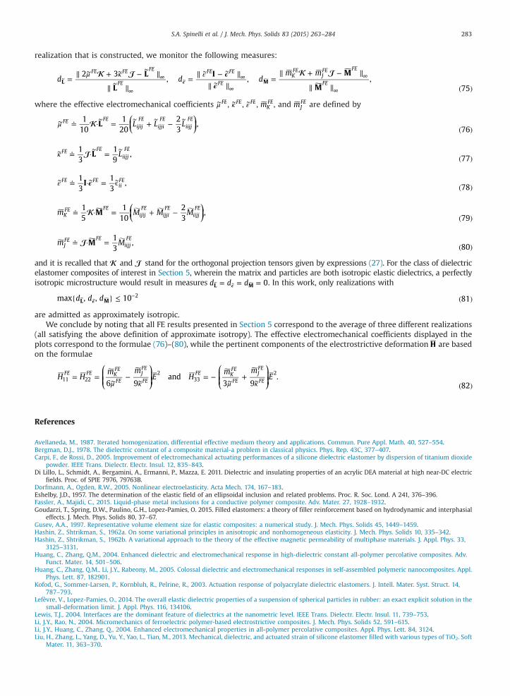
S.A. Spinelli et al. / J. Mech. Phys. Solids 83 (2015) 263–284 283

realization that is constructed, we monitor the following measures:

d d dm mL

L

I M

M

2 3, , ,

75

FE FE FE

FE

FE FE

FEKFE

JFE FE

FEL Mϵ

ϵμ κ ε

=∥ + − ∥

∥ ∥=

∥ − ∥∥ ∥

=∥ + − ∥

∥ ∥ ( )

∼ ∼∼

∼ ∼

∼∼

ϵ∞

∞

∞

∞

∞

∞

∼∼

where the effective electromechanical coefficients FEμ∼ , FEκ∼ , FEε∼ , mKFE , and mJ

FE are defined by

⎛⎝⎜

⎞⎠⎟L L LL

110

120

23

,76

FE FEijijFE

ijjiFE

iijjFE

μ ≐ · = + −( )

∼ ∼ ∼∼∼

LL13

19

, 77FE FE

iijjFE

κ ≐ · = ( )∼ ∼∼

I13

13

, 78FE FE

iiFEϵε ≐ · = ϵ ( )

∼∼ ∼

⎛⎝⎜

⎞⎠⎟m M M MM

15

110

23

,79K

FE FEijijFE

ijjiFE

iijjFE

≐ · = + −( )

m MM13

, 80JFE FE

iijjFE

≐ · = ( )

and it is recalled that and stand for the orthogonal projection tensors given by expressions (27). For the class of dielectricelastomer composites of interest in Section 5, wherein the matrix and particles are both isotropic elastic dielectrics, a perfectlyisotropic microstructure would result in measures d d d 0L M= = =ϵ∼∼ . In this work, only realizations with

d d dmax , , 10 81L M2{ } ≤ ( )ϵ

−∼∼

are admitted as approximately isotropic.We conclude by noting that all FE results presented in Section 5 correspond to the average of three different realizations

(all satisfying the above definition of approximate isotropy). The effective electromechanical coefficients displayed in theplots correspond to the formulae (76)–(80), while the pertinent components of the electrostrictive deformation H are basedon the formulae

⎛⎝⎜⎜

⎞⎠⎟⎟

⎛⎝⎜⎜

⎞⎠⎟⎟H H

m mE H

m mE

6 9and

3 9.

82

FE FE KFE

FEJFE

FEFE K

FE

FEJFE

FE11 222

332

μ κ μ κ= = − = − +

( )∼ ∼∼ ∼

References

Avellaneda, M., 1987. Iterated homogenization, differential effective medium theory and applications. Commun. Pure Appl. Math. 40, 527–554.Bergman, D.J., 1978. The dielectric constant of a composite material-a problem in classical physics. Phys. Rep. 43C, 377–407.Carpi, F., de Rossi, D., 2005. Improvement of electromechanical actuating performances of a silicone dielectric elastomer by dispersion of titanium dioxide

powder. IEEE Trans. Dielectr. Electr. Insul. 12, 835–843.Di Lillo, L., Schmidt, A., Bergamini, A., Ermanni, P., Mazza, E. 2011. Dielectric and insulating properties of an acrylic DEA material at high near-DC electric

fields. Proc. of SPIE 7976, 79763B.Dorfmann, A., Ogden, R.W., 2005. Nonlinear electroelasticity. Acta Mech. 174, 167–183.Eshelby, J.D., 1957. The determination of the elastic field of an ellipsoidal inclusion and related problems. Proc. R. Soc. Lond. A 241, 376–396.Fassler, A., Majidi, C., 2015. Liquid-phase metal inclusions for a conductive polymer composite. Adv. Mater. 27, 1928–1932.Goudarzi, T., Spring, D.W., Paulino, G.H., Lopez-Pamies, O. 2015. Filled elastomers: a theory of filler reinforcement based on hydrodynamic and interphasial

effects. J. Mech. Phys. Solids 80, 37–67.Gusev, A.A., 1997. Representative volume element size for elastic composites: a numerical study. J. Mech. Phys. Solids 45, 1449–1459.Hashin, Z., Shtrikman, S., 1962a. On some variational principles in anisotropic and nonhomogeneous elasticity. J. Mech. Phys. Solids 10, 335–342.Hashin, Z., Shtrikman, S., 1962b. A variational approach to the theory of the effective magnetic permeability of multiphase materials. J. Appl. Phys. 33,

3125–3131.Huang, C., Zhang, Q.M., 2004. Enhanced dielectric and electromechanical response in high-dielectric constant all-polymer percolative composites. Adv.

Funct. Mater. 14, 501–506.Huang, C., Zhang, Q.M., Li, J.Y., Rabeony, M., 2005. Colossal dielectric and electromechanical responses in self-assembled polymeric nanocomposites. Appl.

Phys. Lett. 87, 182901.Kofod, G., Sommer-Larsen, P., Kornbluh, R., Pelrine, R., 2003. Actuation response of polyacrylate dielectric elastomers. J. Intell. Mater. Syst. Struct. 14,

787–793.Lefèvre, V., Lopez-Pamies, O., 2014. The overall elastic dielectric properties of a suspension of spherical particles in rubber: an exact explicit solution in the

small-deformation limit. J. Appl. Phys. 116, 134106.Lewis, T.J., 2004. Interfaces are the dominant feature of dielectrics at the nanometric level. IEEE Trans. Dielectr. Electr. Insul. 11, 739–753.Li, J.Y., Rao, N., 2004. Micromechanics of ferroelectric polymer-based electrostrictive composites. J. Mech. Phys. Solids 52, 591–615.Li, J.Y., Huang, C., Zhang, Q., 2004. Enhanced electromechanical properties in all-polymer percolative composites. Appl. Phys. Lett. 84, 3124.Liu, H., Zhang, L., Yang, D., Yu, Y., Yao, L., Tian, M., 2013. Mechanical, dielectric, and actuated strain of silicone elastomer filled with various types of TiO2. Soft

Mater. 11, 363–370.

S.A. Spinelli et al. / J. Mech. Phys. Solids 83 (2015) 263–284284

Lopez-Pamies, O., 2006. On the Effective Behavior, Microstructure Evolution, and Macroscopic Stability of Elastomeric Composites (Ph.D. dissertation).University of Pennsylvania, USA.

Lopez-Pamies, O., 2014. Elastic dielectric composites: theory and application to particle-filled ideal dielectrics. J. Mech. Phys. Solids 64, 61–82.Lopez-Pamies, O., Goudarzi, T., Nakamura, T., 2013a. The nonlinear elastic response of suspensions of rigid inclusions in rubber: I—an exact result for dilute

suspensions. J. Mech. Phys. Solids 61, 1–18.Lopez-Pamies, O., Goudarzi, T., Nakamura, T., 2013b. The nonlinear elastic response of suspensions of rigid inclusions in rubber: II—a simple explicit

approximation for finite-concentration suspensions. J. Mech. Phys. Solids 61, 19–37.Lopez-Pamies, O., Goudarzi, T., Meddeb, A.B., Ounaies, Z., 2014. Extreme enhancement and reduction of the dielectric response of polymer nanoparticulate

composites via interphasial charges. Appl. Phys. Lett. 104, 24290.MATLAB Version 8.3 Documentation, Mathworks, Natick, Massachusetts, USA, 2014.Mc Carthy, D.N., Risse, S., Katekomol, P., Kofod, G., 2009. The effect of dispersion on the increased relative permittivity of TiO2/SEBS composites. J. Phys. D:

Appl. Phys. 42, 145406.Michel, J.C., Moulinec, H., Suquet, P., 1999. Effective properties of composite materials with periodic microstructure: a computational approach. Comput.

Methods Appl. Mech. Eng. 172, 109–143.Milton, G.W., 2002. The theory of composites. Cambridge Monographs on Applied and Computational Mathematics, 6. Cambridge University Press,

Cambridge.Roy, M., Nelson, J.K., MacCrone, R.K., Schadler, L.S., Reed, C.W., Keefe, R., Zenger, W., 2005. Polymer nanocomposite dielectrics—the role of the interface. IEEE

Trans. Dielectr. Electr. Insul. 12, 629–643.Schöberl, J., 1997. Netgen an advancing front 2d/3d-mesh generator based on abstract rules. Comput. Vis. Sci. 1, 41–52.Segurado, J., Llorca, J., 2002. A numerical approximation to the elastic properties of sphere-reinforced composites. J. Mech. Phys. Solids 50, 2107–2121.Siboni, M.H., Ponte Castañeda, P., 2013. Dielectric elastomer composites: small-deformation theory and applications. Philos. Mag. 93, 2769–2801.Spinelli, S.A., Lopez-Pamies, O., 2014. A general closed-form solution for the overall response of piezoelectric composites with periodic and random

particulate microstructures. Int. J. Solids Struct. 51, 2979–2989.Stratton, J.S., 1941. Electromagnetic Theory. McGraw-Hill, New York, London.Suo, Z., Zhao, X., Greene, W.H., 2008. A nonlinear field theory of deformable dielectrics. J. Mech. Phys. Solids 56, 467–486.Tian, L., 2007. Effective Behavior of Dielectric Elastomer Composites (Ph.D. thesis). California Institute of Technology.Tian, L., Tevet-Deree, L., deBotton, G., Bhattacharya, K., 2012. Dielectric elastomer composites. J. Mech. Phys. Solids 60, 181–198.Toupin, R.A., 1956. The elastic dielectric. J. Ration. Mech. Anal. 5, 849–915.Wang, Q., Suo, Z., Zhao, X., 2012. Bursting drops in solid dielectrics caused by high voltages. Nat. Commun. 3, 1157.Willis, J.R., 1977. Bounds and self-consistent estimates for the overall moduli of anisotropic composites. J. Mech. Phys. Solids 25, 185–202.Wissler, M., Mazza, E., 2007. Electromechanical coupling in dielectric elastomer actuators. Sens. Actuators A 138, 384–393.Zhang, Q.M., Hengfeng, L., Poh, M., Xia, F., Cheng, Z.-Y., Xu, H., Huang, C., 2002. An all-organic composite actuator material with high dielectric constant.

Nature 419, 284–287.