rsos.royalsocietypublishing.org

ResearchCite this article: Chan A, Tuszynski JA. 2016Automatic prediction of tumour malignancy inbreast cancer with fractal dimension. R. Soc.open sci. 3: 160558.http://dx.doi.org/10.1098/rsos.160558

Received: 30 August 2016Accepted: 7 November 2016

Subject Category:Biology (whole organism)

Subject Areas:computational biology/health and disease andepidemiology/computer modelling andsimulation

Keywords:cancer prediction, tumour malignancy,automatic image slide analysis, fractaldimension

Author for correspondence:Jack A. Tuszynskie-mail: jack.tuszynski@gmail.com

Automatic prediction oftumour malignancy inbreast cancer with fractaldimensionAlan Chan3 and Jack A. Tuszynski1,2

1Department of Oncology, University of Alberta, 11560 University Avenue, Edmonton,Alberta, Canada T6G 1Z22Department of Physics, University of Alberta, Centennial Centre for InterdisciplinaryScience, Edmonton, Alberta, Canada T6G 2E13Department of Mathematical and Statistical Sciences, University of Alberta, CentralAcademic Building, Edmonton, Alberta, Canada T6G 2G1

JAT, 0000-0001-9976-0429

Breast cancer is one of the most prevalent types of cancer todayin women. The main avenue of diagnosis is through manualexamination of histopathology tissue slides. Such a process isoften subjective and error-ridden, suffering from both inter-and intraobserver variability. Our objective is to develop anautomatic algorithm for analysing histopathology slides freeof human subjectivity. Here, we calculate the fractal dimensionof images of numerous breast cancer slides, at magnificationsof 40×, 100×, 200× and 400×. Using machine learning,specifically, the support vector machine (SVM) method, the F1score for classification accuracy of the 40× slides was found tobe 0.979. Multiclass classification on the 40× slides yielded anaccuracy of 0.556. A reduction of the size and scope of the SVMtraining set gave an average F1 score of 0.964. Taken together,these results show great promise in the use of fractal dimensionto predict tumour malignancy.

1. IntroductionExponential increase in technological capability owing to thescope of information technology applications over the pastfew decades has revolutionized the way modern societyfunctions, especially in terms of communication. The advent ofcomputerization has automated many tasks once seen to be onlyin the realm of manual labour. At the same time, advances inmedical knowledge have allowed us to determine with evergreater precision the particular characteristics of the ailmentsthat afflict us, as well as improved treatments to ameliorate ourlives. The diagnosis of cancer is one area of medicine that is

2016 The Authors. Published by the Royal Society under the terms of the Creative CommonsAttribution License http://creativecommons.org/licenses/by/4.0/, which permits unrestricteduse, provided the original author and source are credited.

on July 9, 2018http://rsos.royalsocietypublishing.org/Downloaded from

2

rsos.royalsocietypublishing.orgR.Soc.opensci.3:160558

................................................amenable to automation but so far has been largely dependent on the traditional approaches, using theexpertise of trained professionals.

Histological evaluation of a tissue sample is a critical step in the diagnosis of cancer, providingimportant prognostic information [1,2]. However, significant inter- and intravariability exists betweenpathologists [3,4], especially in ‘borderline’ cases [5]. Indeed, different diagnoses can drastically changethe treatment options chosen for patients and substantially affect the outcomes [4]. Therefore, it is clearlyof significance to maximize the reliability of histological evaluation to be more in line with the use ofcomputerized methods that have improved the quality in many areas of technology, including medicalimaging. There are at least two ways in which to improve histological evaluation: the development of aquantitative measure sufficiently well-linked to cancer severity and the use of an automated program tomake objective calculations of such a measure. This paper intends to propose some algorithms that canbe used in this connection.

2. Background2.1. Past workThere have been many attempts to automate the diagnosis of cancer from histology slides. Commonto all is a three-step process: (i) preprocessing of the image, (ii) extraction of relevant features, and(iii) diagnosis from those features [6]. The step of greatest interest, with perhaps the greatest diversityin methods, is the feature extraction step. The goal here is to select features of an image that may beamenable to quantification and subsequent computational analysis, while at the same time being goodmeasures of cancer severity. That is, the hope is to correlate an image feature with either a diagnostic ora prognostic indicator, including, but not limited to, tumour malignancy and a related survival rate.

A plethora of features have been proposed and tested in the context of histopathology of cancer,namely fractal dimension [7–10], entropy [11], textural features based on the image histogram [12], andeven features that were automatically selected by an unsupervised machine learning algorithm [13].Often, a large number of features are used at the same time [14,15]. In this paper, we focus on furthertesting of fractal dimension as a viable image feature that can lead to a high level of confidence inthe resultant classification. We extend the work done previously on this particular feature by testingon a larger dataset that has been selected for its consistency and quality, applying machine learningfor prediction of tumour malignancy, and running further classification procedures to increase ourconfidence in the extent to which our hypothesis may be generalized.

2.2. Fractal dimensionTo best understand what fractal dimension is, it is helpful to start with the familiar notion of topologicaldimension in geometry. A line has topological dimension 1, a square has topological dimension 2 anda cube has topological dimension 3. Intuitively, topological dimension is a measure of how everyday,regular objects change with scaling, and is usually an integral value. A metre stick of length 1 m isrequired to measure a 1 m line. If we use a half-metre stick, then double the number sticks will be requiredto measure the line. Similarly, we may use a square of side length 1 m to measure the same square of sidelength 1 m. If we halve the length of the measuring square, then we now require four squares to measurethe full 1 m × 1 m square. More concretely,

N = ε−d, (2.1)

where N is the number of sticks required, ε is the scaling factor and d is the topological dimension.Solving for d,

d = − log(N)log(ε)

. (2.2)

Regarding our square example, we have d = −log(4)/(log(1/2)) = 2 which is what we expect thedimension of a two-dimensional image to be. In figure 1, we show an example of a geometrical fractalwhich is called the Koch snowflake whose fractal dimension is approximately 1.26.

However, nature often does not conform to the pristine regularity of Euclidean geometry. In particular,there are objects whose dimension is not integral, but real-valued, accompanied by unexpected scalingbehaviour. We label such d ∈ R the fractal dimension. Qualitatively, non-integral fractal dimension maybe visually recognizable by a more complex image border, and self-similarity after scaling. Indeed, the‘fractal’ of fractal dimension refers to the often unusual scaling behaviour of fractal objects, which may

on July 9, 2018http://rsos.royalsocietypublishing.org/Downloaded from

3

rsos.royalsocietypublishing.orgR.Soc.opensci.3:160558

................................................

Figure 1. An image of the Koch snowflake, a fractal with fractal dimension d ≈ 1.26. From https://commons.wikimedia.org/wiki/File:Flocke.PNG, licensed under Creative Commons.

be both geometrical and physical. The former are created by applying an iterative rule to a motif whilethe latter are created by a physical process such as diffusion-limited aggregation or a biological processsuch as tumour growth, for example.

In fact, the fractal dimension of any image on a two-dimensional surface will always satisfy d ∈ [1, 2].That is, the dimension of the image is bounded above by 2, the dimension of the containing environment,and bounded below by 1, the dimension of any closed curve on the two-dimensional surface.

The obvious question is how one goes about calculating fractal dimension. In this paper, we use thebox-counting algorithm. The procedure is described in great detail in [16], but we briefly explain it herefor the reader’s benefit.

A series of boxes of side length ε are fitted, without overlap, over the image to be analysed. Thenumber of boxes that contain some portion of the image are then counted. The logarithm of that numberis divided by the negative logarithm of the size of the boxes used. We, therefore, have

db = limε→0

− log(N(ε))log(ε)

= limε→0

log(N(ε))log(1/ε)

, (2.3)

where N(ε) denotes the number of non-empty boxes of side length ε. There is a clear connection betweenthis formula and that of the original definition of fractal dimension. Because we cannot apply a limitoperation to images that do not have an infinite precision in detail, we instead calculate −log(N(ε))/log(ε)for various values of ε, and find the slope of log(N(ε)) plotted against log(1/ε).

We have mentioned the Koch fractal only as an example. Its fractal dimension of 1.26 is relatively low,as will be shown below, by comparison with the fractal dimensions of the pathology slides analysedhere. Another type of geometrical fractal, the so-called Cesaro curve, may be a closer geometricalapproximation to pathology images, owing to its fractal dimension which is close to 2.0 depending onthe angle between the line segments in its motif. More information about fractals and their propertiesmay be found in [17].

3. DataIn order to examine the viability of using the fractal dimension for histopathology of breast cancer,we have decided to use the BreaKHIS database in this study. This database has a high degreeof consistency and image quality that was important in making the subsequent results free ofartefacts. It is a sufficiently large dataset to allow for statistical significance because it consists of7909 breast cancer histopathology images, acquired from 82 patients by [18], publicly available fromhttp://web.inf.ufpr.br/vri/breast-cancer-database. It is a freely available Web-based dataset, and weencourage the interested reader to access these data for inspection. Images were collected through aclinical study from January 2014 to December 2014. Samples were taken from breast tissue biopsy slides,and are all stained with haematoxylin and eosin (H&E). Owing to the internal consistency of the images,we were able to avoid dealing with such common problems as image artefacts, e.g. colour batch effects.The BreaKHIS dataset includes both benign and malignant images, at magnifications of 40×, 100×, 200×and 400×. A tally is in table 1. Each image is 700 × 460 pixels, and is of the PNG image file format.

on July 9, 2018http://rsos.royalsocietypublishing.org/Downloaded from

4

rsos.royalsocietypublishing.orgR.Soc.opensci.3:160558

................................................A F PT TA

DC LC MC PC

Figure 2. Representative benign and malignant images at 40× magnification. Benign: adenosis (A), fibroadenoma (F), phyllodestumour (PT) and tubular adenoma (TA). Malignant: ductal carcinoma (DC), lobular carcinoma (LC), mucinous carcinoma (MC) andpapillary carcinoma (PC).

Table 1. The distribution of images in BreaKHIS, from [18].

magnification benign malignant total

40× 625 1370 1995. . . . . . . . . . . . . . . . . . . . . . . . . . . . . . . . . . . . . . . . . . . . . . . . . . . . . . . . . . . . . . . . . . . . . . . . . . . . . . . . . . . . . . . . . . . . . . . . . . . . . . . . . . . . . . . . . . . . . . . . . . . . . . . . . . . . . . . . . . . . . . . . . . . . . . . . . . . . . . . . . . . . . . . . . . . . . . . . . . . . . . . . . . . . . . . . . . . . . . . . . . . . . . . . . . . . . . . . .

100× 644 1437 2081. . . . . . . . . . . . . . . . . . . . . . . . . . . . . . . . . . . . . . . . . . . . . . . . . . . . . . . . . . . . . . . . . . . . . . . . . . . . . . . . . . . . . . . . . . . . . . . . . . . . . . . . . . . . . . . . . . . . . . . . . . . . . . . . . . . . . . . . . . . . . . . . . . . . . . . . . . . . . . . . . . . . . . . . . . . . . . . . . . . . . . . . . . . . . . . . . . . . . . . . . . . . . . . . . . . . . . . . .

200× 623 1390 2013. . . . . . . . . . . . . . . . . . . . . . . . . . . . . . . . . . . . . . . . . . . . . . . . . . . . . . . . . . . . . . . . . . . . . . . . . . . . . . . . . . . . . . . . . . . . . . . . . . . . . . . . . . . . . . . . . . . . . . . . . . . . . . . . . . . . . . . . . . . . . . . . . . . . . . . . . . . . . . . . . . . . . . . . . . . . . . . . . . . . . . . . . . . . . . . . . . . . . . . . . . . . . . . . . . . . . . . . .

400× 588 1232 1820. . . . . . . . . . . . . . . . . . . . . . . . . . . . . . . . . . . . . . . . . . . . . . . . . . . . . . . . . . . . . . . . . . . . . . . . . . . . . . . . . . . . . . . . . . . . . . . . . . . . . . . . . . . . . . . . . . . . . . . . . . . . . . . . . . . . . . . . . . . . . . . . . . . . . . . . . . . . . . . . . . . . . . . . . . . . . . . . . . . . . . . . . . . . . . . . . . . . . . . . . . . . . . . . . . . . . . . . .

total 2480 5429 7909. . . . . . . . . . . . . . . . . . . . . . . . . . . . . . . . . . . . . . . . . . . . . . . . . . . . . . . . . . . . . . . . . . . . . . . . . . . . . . . . . . . . . . . . . . . . . . . . . . . . . . . . . . . . . . . . . . . . . . . . . . . . . . . . . . . . . . . . . . . . . . . . . . . . . . . . . . . . . . . . . . . . . . . . . . . . . . . . . . . . . . . . . . . . . . . . . . . . . . . . . . . . . . . . . . . . . . . . .

no. patients 24 58 82. . . . . . . . . . . . . . . . . . . . . . . . . . . . . . . . . . . . . . . . . . . . . . . . . . . . . . . . . . . . . . . . . . . . . . . . . . . . . . . . . . . . . . . . . . . . . . . . . . . . . . . . . . . . . . . . . . . . . . . . . . . . . . . . . . . . . . . . . . . . . . . . . . . . . . . . . . . . . . . . . . . . . . . . . . . . . . . . . . . . . . . . . . . . . . . . . . . . . . . . . . . . . . . . . . . . . . . . .

Table 2. The distribution of images of benign tumours in BreaKHIS, from [18].

magnification A F TA PT total

40× 114 253 109 149 625. . . . . . . . . . . . . . . . . . . . . . . . . . . . . . . . . . . . . . . . . . . . . . . . . . . . . . . . . . . . . . . . . . . . . . . . . . . . . . . . . . . . . . . . . . . . . . . . . . . . . . . . . . . . . . . . . . . . . . . . . . . . . . . . . . . . . . . . . . . . . . . . . . . . . . . . . . . . . . . . . . . . . . . . . . . . . . . . . . . . . . . . . . . . . . . . . . . . . . . . . . . . . . . . . . . . . . . . .

100× 113 260 121 150 644. . . . . . . . . . . . . . . . . . . . . . . . . . . . . . . . . . . . . . . . . . . . . . . . . . . . . . . . . . . . . . . . . . . . . . . . . . . . . . . . . . . . . . . . . . . . . . . . . . . . . . . . . . . . . . . . . . . . . . . . . . . . . . . . . . . . . . . . . . . . . . . . . . . . . . . . . . . . . . . . . . . . . . . . . . . . . . . . . . . . . . . . . . . . . . . . . . . . . . . . . . . . . . . . . . . . . . . . .

200× 111 264 108 140 623. . . . . . . . . . . . . . . . . . . . . . . . . . . . . . . . . . . . . . . . . . . . . . . . . . . . . . . . . . . . . . . . . . . . . . . . . . . . . . . . . . . . . . . . . . . . . . . . . . . . . . . . . . . . . . . . . . . . . . . . . . . . . . . . . . . . . . . . . . . . . . . . . . . . . . . . . . . . . . . . . . . . . . . . . . . . . . . . . . . . . . . . . . . . . . . . . . . . . . . . . . . . . . . . . . . . . . . . .

400× 106 237 115 130 588. . . . . . . . . . . . . . . . . . . . . . . . . . . . . . . . . . . . . . . . . . . . . . . . . . . . . . . . . . . . . . . . . . . . . . . . . . . . . . . . . . . . . . . . . . . . . . . . . . . . . . . . . . . . . . . . . . . . . . . . . . . . . . . . . . . . . . . . . . . . . . . . . . . . . . . . . . . . . . . . . . . . . . . . . . . . . . . . . . . . . . . . . . . . . . . . . . . . . . . . . . . . . . . . . . . . . . . . .

total 444 1014 453 569 2368. . . . . . . . . . . . . . . . . . . . . . . . . . . . . . . . . . . . . . . . . . . . . . . . . . . . . . . . . . . . . . . . . . . . . . . . . . . . . . . . . . . . . . . . . . . . . . . . . . . . . . . . . . . . . . . . . . . . . . . . . . . . . . . . . . . . . . . . . . . . . . . . . . . . . . . . . . . . . . . . . . . . . . . . . . . . . . . . . . . . . . . . . . . . . . . . . . . . . . . . . . . . . . . . . . . . . . . . .

no. patients 4 10 3 7 24. . . . . . . . . . . . . . . . . . . . . . . . . . . . . . . . . . . . . . . . . . . . . . . . . . . . . . . . . . . . . . . . . . . . . . . . . . . . . . . . . . . . . . . . . . . . . . . . . . . . . . . . . . . . . . . . . . . . . . . . . . . . . . . . . . . . . . . . . . . . . . . . . . . . . . . . . . . . . . . . . . . . . . . . . . . . . . . . . . . . . . . . . . . . . . . . . . . . . . . . . . . . . . . . . . . . . . . . .

Table 3. The distribution of images of malignant tumours in BreaKHIS, from [18].

magnification DC LC MC PC total

40× 864 156 205 145 1370. . . . . . . . . . . . . . . . . . . . . . . . . . . . . . . . . . . . . . . . . . . . . . . . . . . . . . . . . . . . . . . . . . . . . . . . . . . . . . . . . . . . . . . . . . . . . . . . . . . . . . . . . . . . . . . . . . . . . . . . . . . . . . . . . . . . . . . . . . . . . . . . . . . . . . . . . . . . . . . . . . . . . . . . . . . . . . . . . . . . . . . . . . . . . . . . . . . . . . . . . . . . . . . . . . . . . . . . .

100× 903 170 222 142 1437. . . . . . . . . . . . . . . . . . . . . . . . . . . . . . . . . . . . . . . . . . . . . . . . . . . . . . . . . . . . . . . . . . . . . . . . . . . . . . . . . . . . . . . . . . . . . . . . . . . . . . . . . . . . . . . . . . . . . . . . . . . . . . . . . . . . . . . . . . . . . . . . . . . . . . . . . . . . . . . . . . . . . . . . . . . . . . . . . . . . . . . . . . . . . . . . . . . . . . . . . . . . . . . . . . . . . . . . .

200× 896 163 196 135 1390. . . . . . . . . . . . . . . . . . . . . . . . . . . . . . . . . . . . . . . . . . . . . . . . . . . . . . . . . . . . . . . . . . . . . . . . . . . . . . . . . . . . . . . . . . . . . . . . . . . . . . . . . . . . . . . . . . . . . . . . . . . . . . . . . . . . . . . . . . . . . . . . . . . . . . . . . . . . . . . . . . . . . . . . . . . . . . . . . . . . . . . . . . . . . . . . . . . . . . . . . . . . . . . . . . . . . . . . .

400× 788 137 169 138 1232. . . . . . . . . . . . . . . . . . . . . . . . . . . . . . . . . . . . . . . . . . . . . . . . . . . . . . . . . . . . . . . . . . . . . . . . . . . . . . . . . . . . . . . . . . . . . . . . . . . . . . . . . . . . . . . . . . . . . . . . . . . . . . . . . . . . . . . . . . . . . . . . . . . . . . . . . . . . . . . . . . . . . . . . . . . . . . . . . . . . . . . . . . . . . . . . . . . . . . . . . . . . . . . . . . . . . . . . .

total 3451 626 792 560 5429. . . . . . . . . . . . . . . . . . . . . . . . . . . . . . . . . . . . . . . . . . . . . . . . . . . . . . . . . . . . . . . . . . . . . . . . . . . . . . . . . . . . . . . . . . . . . . . . . . . . . . . . . . . . . . . . . . . . . . . . . . . . . . . . . . . . . . . . . . . . . . . . . . . . . . . . . . . . . . . . . . . . . . . . . . . . . . . . . . . . . . . . . . . . . . . . . . . . . . . . . . . . . . . . . . . . . . . . .

no. patients 38 5 9 6 58. . . . . . . . . . . . . . . . . . . . . . . . . . . . . . . . . . . . . . . . . . . . . . . . . . . . . . . . . . . . . . . . . . . . . . . . . . . . . . . . . . . . . . . . . . . . . . . . . . . . . . . . . . . . . . . . . . . . . . . . . . . . . . . . . . . . . . . . . . . . . . . . . . . . . . . . . . . . . . . . . . . . . . . . . . . . . . . . . . . . . . . . . . . . . . . . . . . . . . . . . . . . . . . . . . . . . . . . .

Furthermore, the benign and malignant images are split into subtypes. The benign tumour imagescontain slides of adenosis (A), fibroadenoma (F), phyllodes tumour (PT) and tubular adenoma (TA). Themalignant tumour images contain slides of ductal carcinoma (DC), lobular carcinoma (LC), mucinous

on July 9, 2018http://rsos.royalsocietypublishing.org/Downloaded from

5

rsos.royalsocietypublishing.orgR.Soc.opensci.3:160558

................................................carcinoma (MC) and papillary carcinoma (PC). In figure 2, we show representative images of eachsubtype. In tables 1–3, we summarize the distribution of images in the BreaKHIS database for benignand malignant cases as well as into the above subtypes.

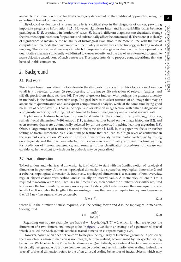
4. MethodMATHEMATICA was the programming environment used in this study. Fortunately, this programmingtool has an edge detection tool that allows one to find sharp boundaries between different areas of animage. First, fractal dimensions for all 7909 images were calculated. This process was accomplished inseveral steps described below.

1. Binarize all images and detect the edges, with MATHEMATICA’S built-in functions Binarize andEdgeDetect.

2. Calculate the integral image of each image. The process is detailed in [19]. The calculation of theintegral image is not necessary, but vastly speeds up the algorithm by allowing quick calculationof the number of pixels in a given box.

3. We take ε from three pixels to four pixels, with a step size of only 1. While this decision gives onlytwo data points, the results of our study justify our choice. Furthermore, the usage of larger sidelengths would have introduced misleading values for the fractal dimension into our calculations.

4. For each ε, the image is partitioned into non-overlapping boxes of side length ε. The number ofpixels in a given box is calculated from the integral image. The total number of non-empty boxesis summed, and put into an ordered pair with 1/ε. We then take the logarithm of both values.

5. The fractal dimension of each image is calculated by fitting a straight line to the just-calculateddata points of each image, and recording the slope of the line as the fractal dimension of theimage. The MATHEMATICA function Fit was used in this step.

Without loss of generality, we describe the procedure taken with the 40× slides. Figure 3 is an examplethat can be used as a reference. Similar steps were taken in the remaining cases. We used a randomlyselected set consisting of 50% of the benign tumour fractal dimensions and a randomly selected setconsisting of 50% of the malignant tumour fractal dimension as a training set, setting aside the restof the data for use as a validation set. We trained a support vector machine (SVM) algorithm, on thetraining set, to classify whether a tumour was benign or malignant based solely on fractal dimension.Strictly speaking, because we had only one image feature, an SVM was not absolutely necessary. Indeed,a cut-off fractal dimension value could have been found by hand. However, in the interests of precisionand certainty, we chose to use an SVM. Obviously, other machine-learning methods can be used here andwill most likely be equally successful in their performance. Moreover, with only one feature used, onecould indeed resort to classical linear discriminant analysis between clouds of points using for exampleMahalanobis distance [20] to replace a somewhat arbitrary determination of the cut-off dimension.

From the results of the SVM predictions on the validation set, we decided whether or not to continuewith further classification trials. Further trials were only pursued with the 40× slides.

A multiclass classification was then attempted. Instead of classifying the 40× slides by benign versusmalignant, we tried to classify the images based on the eight subtypes of benign and malignant tumours.That is, we predicted the tumour subtype to which a given tissue image belonged. A random half of thefractal dimensions of each subtype served as a training set.

Afterwards, we performed another classification trial, this time modifying the size of the training set.In total, 16 different SVMs were trained, each using a different training set. For each SVM, the training setconsisted of the fractal dimensions of a single benign subtype, and a single malignant subtype. Becausethere are four benign subtypes and four malignant subtypes, we have 16 different possible combinationsfor the training sets, and hence 16 SVMs. The SVMs were then tested against the fractal dimensions uponwhich they were not trained. For example, an SVM was trained against adenoma and ductal carcinoma,and subsequently tested against fibroadenoma, phyllodes tumour, tubular adenoma, lobular carcinoma,mucinous carcinoma and papillary carcinoma.

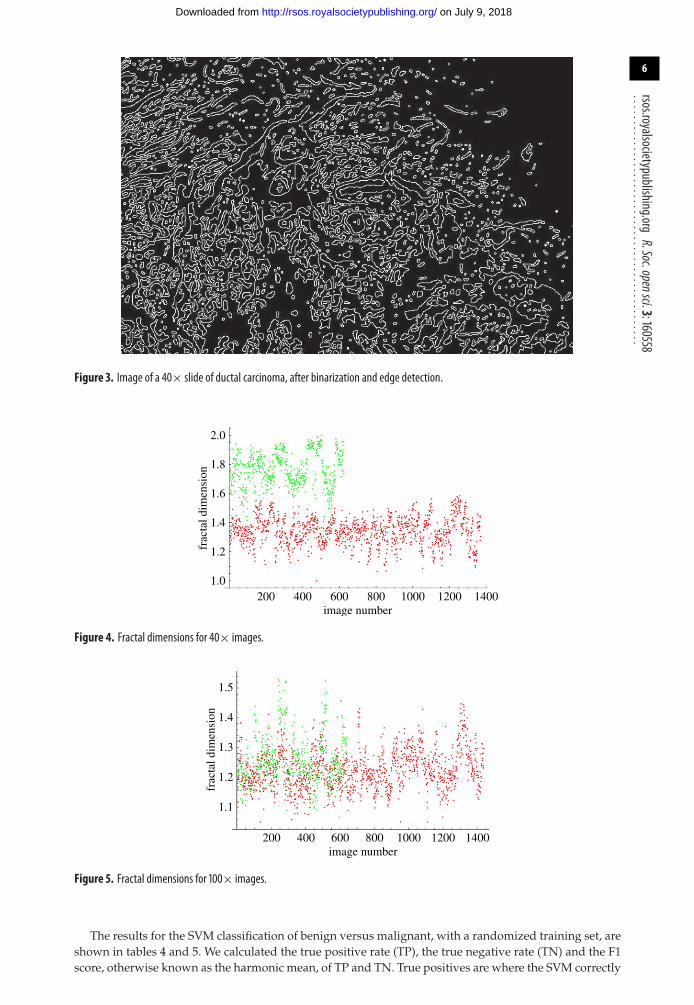
5. ResultsThe fractal dimensions for all images at each magnification are plotted in figures 4–7. The green dotsrepresent benign images, and the red dots represent malignant images. The y-axis corresponds to fractaldimension, and the x-axis corresponds to the arbitrary image numbering.

on July 9, 2018http://rsos.royalsocietypublishing.org/Downloaded from

6

rsos.royalsocietypublishing.orgR.Soc.opensci.3:160558

................................................

Figure 3. Image of a 40× slide of ductal carcinoma, after binarization and edge detection.

2.0

frac

tal d

imen

sion

1.8

1.6

1.4

1.2

1.0200 400 600

image number800 1000 1200 1400

Figure 4. Fractal dimensions for 40× images.

frac

tal d

imen

sion

1.5

1.4

1.3

1.2

1.1

200 400 600image number

800 1000 1200 1400

Figure 5. Fractal dimensions for 100× images.

The results for the SVM classification of benign versus malignant, with a randomized training set, areshown in tables 4 and 5. We calculated the true positive rate (TP), the true negative rate (TN) and the F1score, otherwise known as the harmonic mean, of TP and TN. True positives are where the SVM correctly

on July 9, 2018http://rsos.royalsocietypublishing.org/Downloaded from

7

rsos.royalsocietypublishing.orgR.Soc.opensci.3:160558

................................................

1.4

1.3

1.2

1.1

1.0fr

acta

l dim

ensi

on

200 400 600image number

800 1000 1200 1400

Figure 6. Fractal dimensions for 200× images.

1.4

1.3

1.2

1.1

1.0

frac

tal d

imen

sion

200 400 600image number

800 1000 1200

Figure 7. Fractal dimensions for 400× images.

Table 4. Classification accuracy for benign versus malignant images at all magnifications.

magnification TP TN F1

40× 0.990 0.968 0.979. . . . . . . . . . . . . . . . . . . . . . . . . . . . . . . . . . . . . . . . . . . . . . . . . . . . . . . . . . . . . . . . . . . . . . . . . . . . . . . . . . . . . . . . . . . . . . . . . . . . . . . . . . . . . . . . . . . . . . . . . . . . . . . . . . . . . . . . . . . . . . . . . . . . . . . . . . . . . . . . . . . . . . . . . . . . . . . . . . . . . . . . . . . . . . . . . . . . . . . . . . . . . . . . . . . . . . . . .

100× 0.983 0.090 0.165. . . . . . . . . . . . . . . . . . . . . . . . . . . . . . . . . . . . . . . . . . . . . . . . . . . . . . . . . . . . . . . . . . . . . . . . . . . . . . . . . . . . . . . . . . . . . . . . . . . . . . . . . . . . . . . . . . . . . . . . . . . . . . . . . . . . . . . . . . . . . . . . . . . . . . . . . . . . . . . . . . . . . . . . . . . . . . . . . . . . . . . . . . . . . . . . . . . . . . . . . . . . . . . . . . . . . . . . .

200× 0.974 0.090 0.165. . . . . . . . . . . . . . . . . . . . . . . . . . . . . . . . . . . . . . . . . . . . . . . . . . . . . . . . . . . . . . . . . . . . . . . . . . . . . . . . . . . . . . . . . . . . . . . . . . . . . . . . . . . . . . . . . . . . . . . . . . . . . . . . . . . . . . . . . . . . . . . . . . . . . . . . . . . . . . . . . . . . . . . . . . . . . . . . . . . . . . . . . . . . . . . . . . . . . . . . . . . . . . . . . . . . . . . . .

400× 0.940 0.146 0.253. . . . . . . . . . . . . . . . . . . . . . . . . . . . . . . . . . . . . . . . . . . . . . . . . . . . . . . . . . . . . . . . . . . . . . . . . . . . . . . . . . . . . . . . . . . . . . . . . . . . . . . . . . . . . . . . . . . . . . . . . . . . . . . . . . . . . . . . . . . . . . . . . . . . . . . . . . . . . . . . . . . . . . . . . . . . . . . . . . . . . . . . . . . . . . . . . . . . . . . . . . . . . . . . . . . . . . . . .

classified an image as malignant, and true negatives are where the SVM correctly classified an image asbenign. TP and TN are calculated as ratios between 0 and 1, rounded to three decimal digits. Note that tocalculate the F1 score, we have used the formula: F1 = (2 × TP × TN)/(TP + TN). This harmonic averageformula was used for simplicity and convenience. A different type of averaging can also be applied.

Based on the results in table 4, we chose only to pursue further testing with the 40× fractal dimensions,which gave us the best predictive power. We created another training set containing a random half of theimages of each tumour subtype. Another SVM was trained on this set, and had to classify the rest of theimages based on subtype. Accuracy, the number of correct predictions divided by the total number ofsamples, was 0.556.

Sixteen different SVMs were then trained, with each training set consisting of the fractal dimensionsof a single benign (BT) and single malignant subtype (MT). The SVM then tried to classify the remainingsubtypes by malignancy. As before, we calculated the TN, TP and F1 scores. We re-use the abbreviationsfor the subtypes, repeated here: adenosis (A), fibroadenoma (F), phyllodes tumour (PT) and tubularadenoma (TA). The malignant tumour images contain slides of ductal carcinoma (DC), lobular carcinoma(LC), mucinous carcinoma (C) and papillary carcinoma (PC). The resulting accuracies are in table 5.

on July 9, 2018http://rsos.royalsocietypublishing.org/Downloaded from

8

rsos.royalsocietypublishing.orgR.Soc.opensci.3:160558

................................................Table 5. Benign versus malignant classification accuracy with different training sets.

BT MT TP TN F1

A DC 0.988 0.953 0.970. . . . . . . . . . . . . . . . . . . . . . . . . . . . . . . . . . . . . . . . . . . . . . . . . . . . . . . . . . . . . . . . . . . . . . . . . . . . . . . . . . . . . . . . . . . . . . . . . . . . . . . . . . . . . . . . . . . . . . . . . . . . . . . . . . . . . . . . . . . . . . . . . . . . . . . . . . . . . . . . . . . . . . . . . . . . . . . . . . . . . . . . . . . . . . . . . . . . . . . . . . . . . . . . . . . . . . . . .

A LC 0.993 0.957 0.975. . . . . . . . . . . . . . . . . . . . . . . . . . . . . . . . . . . . . . . . . . . . . . . . . . . . . . . . . . . . . . . . . . . . . . . . . . . . . . . . . . . . . . . . . . . . . . . . . . . . . . . . . . . . . . . . . . . . . . . . . . . . . . . . . . . . . . . . . . . . . . . . . . . . . . . . . . . . . . . . . . . . . . . . . . . . . . . . . . . . . . . . . . . . . . . . . . . . . . . . . . . . . . . . . . . . . . . . .

A MC 0.979 0.967 0.973. . . . . . . . . . . . . . . . . . . . . . . . . . . . . . . . . . . . . . . . . . . . . . . . . . . . . . . . . . . . . . . . . . . . . . . . . . . . . . . . . . . . . . . . . . . . . . . . . . . . . . . . . . . . . . . . . . . . . . . . . . . . . . . . . . . . . . . . . . . . . . . . . . . . . . . . . . . . . . . . . . . . . . . . . . . . . . . . . . . . . . . . . . . . . . . . . . . . . . . . . . . . . . . . . . . . . . . . .

A PC 0.999 0.945 0.971. . . . . . . . . . . . . . . . . . . . . . . . . . . . . . . . . . . . . . . . . . . . . . . . . . . . . . . . . . . . . . . . . . . . . . . . . . . . . . . . . . . . . . . . . . . . . . . . . . . . . . . . . . . . . . . . . . . . . . . . . . . . . . . . . . . . . . . . . . . . . . . . . . . . . . . . . . . . . . . . . . . . . . . . . . . . . . . . . . . . . . . . . . . . . . . . . . . . . . . . . . . . . . . . . . . . . . . . .

F DC 0.982 0.930 0.955. . . . . . . . . . . . . . . . . . . . . . . . . . . . . . . . . . . . . . . . . . . . . . . . . . . . . . . . . . . . . . . . . . . . . . . . . . . . . . . . . . . . . . . . . . . . . . . . . . . . . . . . . . . . . . . . . . . . . . . . . . . . . . . . . . . . . . . . . . . . . . . . . . . . . . . . . . . . . . . . . . . . . . . . . . . . . . . . . . . . . . . . . . . . . . . . . . . . . . . . . . . . . . . . . . . . . . . . .

F LC 0.975 0.946 0.960. . . . . . . . . . . . . . . . . . . . . . . . . . . . . . . . . . . . . . . . . . . . . . . . . . . . . . . . . . . . . . . . . . . . . . . . . . . . . . . . . . . . . . . . . . . . . . . . . . . . . . . . . . . . . . . . . . . . . . . . . . . . . . . . . . . . . . . . . . . . . . . . . . . . . . . . . . . . . . . . . . . . . . . . . . . . . . . . . . . . . . . . . . . . . . . . . . . . . . . . . . . . . . . . . . . . . . . . .

F MC 0.995 0.922 0.957. . . . . . . . . . . . . . . . . . . . . . . . . . . . . . . . . . . . . . . . . . . . . . . . . . . . . . . . . . . . . . . . . . . . . . . . . . . . . . . . . . . . . . . . . . . . . . . . . . . . . . . . . . . . . . . . . . . . . . . . . . . . . . . . . . . . . . . . . . . . . . . . . . . . . . . . . . . . . . . . . . . . . . . . . . . . . . . . . . . . . . . . . . . . . . . . . . . . . . . . . . . . . . . . . . . . . . . . .

F PC 0.999 0.901 0.947. . . . . . . . . . . . . . . . . . . . . . . . . . . . . . . . . . . . . . . . . . . . . . . . . . . . . . . . . . . . . . . . . . . . . . . . . . . . . . . . . . . . . . . . . . . . . . . . . . . . . . . . . . . . . . . . . . . . . . . . . . . . . . . . . . . . . . . . . . . . . . . . . . . . . . . . . . . . . . . . . . . . . . . . . . . . . . . . . . . . . . . . . . . . . . . . . . . . . . . . . . . . . . . . . . . . . . . . .

PT DC 1.000 0.913 0.956. . . . . . . . . . . . . . . . . . . . . . . . . . . . . . . . . . . . . . . . . . . . . . . . . . . . . . . . . . . . . . . . . . . . . . . . . . . . . . . . . . . . . . . . . . . . . . . . . . . . . . . . . . . . . . . . . . . . . . . . . . . . . . . . . . . . . . . . . . . . . . . . . . . . . . . . . . . . . . . . . . . . . . . . . . . . . . . . . . . . . . . . . . . . . . . . . . . . . . . . . . . . . . . . . . . . . . . . .

PT LC 0.993 0.942 0.967. . . . . . . . . . . . . . . . . . . . . . . . . . . . . . . . . . . . . . . . . . . . . . . . . . . . . . . . . . . . . . . . . . . . . . . . . . . . . . . . . . . . . . . . . . . . . . . . . . . . . . . . . . . . . . . . . . . . . . . . . . . . . . . . . . . . . . . . . . . . . . . . . . . . . . . . . . . . . . . . . . . . . . . . . . . . . . . . . . . . . . . . . . . . . . . . . . . . . . . . . . . . . . . . . . . . . . . . .

PT MC 0.999 0.913 0.954. . . . . . . . . . . . . . . . . . . . . . . . . . . . . . . . . . . . . . . . . . . . . . . . . . . . . . . . . . . . . . . . . . . . . . . . . . . . . . . . . . . . . . . . . . . . . . . . . . . . . . . . . . . . . . . . . . . . . . . . . . . . . . . . . . . . . . . . . . . . . . . . . . . . . . . . . . . . . . . . . . . . . . . . . . . . . . . . . . . . . . . . . . . . . . . . . . . . . . . . . . . . . . . . . . . . . . . . .

PT PC 1.000 0.895 0.945. . . . . . . . . . . . . . . . . . . . . . . . . . . . . . . . . . . . . . . . . . . . . . . . . . . . . . . . . . . . . . . . . . . . . . . . . . . . . . . . . . . . . . . . . . . . . . . . . . . . . . . . . . . . . . . . . . . . . . . . . . . . . . . . . . . . . . . . . . . . . . . . . . . . . . . . . . . . . . . . . . . . . . . . . . . . . . . . . . . . . . . . . . . . . . . . . . . . . . . . . . . . . . . . . . . . . . . . .

TA DC 0.992 0.956 0.974. . . . . . . . . . . . . . . . . . . . . . . . . . . . . . . . . . . . . . . . . . . . . . . . . . . . . . . . . . . . . . . . . . . . . . . . . . . . . . . . . . . . . . . . . . . . . . . . . . . . . . . . . . . . . . . . . . . . . . . . . . . . . . . . . . . . . . . . . . . . . . . . . . . . . . . . . . . . . . . . . . . . . . . . . . . . . . . . . . . . . . . . . . . . . . . . . . . . . . . . . . . . . . . . . . . . . . . . .

TA LC 0.974 0.975 0.974. . . . . . . . . . . . . . . . . . . . . . . . . . . . . . . . . . . . . . . . . . . . . . . . . . . . . . . . . . . . . . . . . . . . . . . . . . . . . . . . . . . . . . . . . . . . . . . . . . . . . . . . . . . . . . . . . . . . . . . . . . . . . . . . . . . . . . . . . . . . . . . . . . . . . . . . . . . . . . . . . . . . . . . . . . . . . . . . . . . . . . . . . . . . . . . . . . . . . . . . . . . . . . . . . . . . . . . . .

TA MC 0.994 0.960 0.977. . . . . . . . . . . . . . . . . . . . . . . . . . . . . . . . . . . . . . . . . . . . . . . . . . . . . . . . . . . . . . . . . . . . . . . . . . . . . . . . . . . . . . . . . . . . . . . . . . . . . . . . . . . . . . . . . . . . . . . . . . . . . . . . . . . . . . . . . . . . . . . . . . . . . . . . . . . . . . . . . . . . . . . . . . . . . . . . . . . . . . . . . . . . . . . . . . . . . . . . . . . . . . . . . . . . . . . . .

TA PC 0.999 0.954 0.976. . . . . . . . . . . . . . . . . . . . . . . . . . . . . . . . . . . . . . . . . . . . . . . . . . . . . . . . . . . . . . . . . . . . . . . . . . . . . . . . . . . . . . . . . . . . . . . . . . . . . . . . . . . . . . . . . . . . . . . . . . . . . . . . . . . . . . . . . . . . . . . . . . . . . . . . . . . . . . . . . . . . . . . . . . . . . . . . . . . . . . . . . . . . . . . . . . . . . . . . . . . . . . . . . . . . . . . . .

mean 0.964. . . . . . . . . . . . . . . . . . . . . . . . . . . . . . . . . . . . . . . . . . . . . . . . . . . . . . . . . . . . . . . . . . . . . . . . . . . . . . . . . . . . . . . . . . . . . . . . . . . . . . . . . . . . . . . . . . . . . . . . . . . . . . . . . . . . . . . . . . . . . . . . . . . . . . . . . . . . . . . . . . . . . . . . . . . . . . . . . . . . . . . . . . . . . . . . . . . . . . . . . . . . . . . . . . . . . . . . .

6. DiscussionThe plots shown in figures 4–7 show visually the results of table 4. It is clear that with just fractaldimension as the sole feature, the best hope for diagnostic application is through examination of 40×slides. A possible explanation is that as one increases the magnification, it becomes more difficultto see higher-level features of the cell morphology that are often indicative of cancer, like poor celldifferentiation, and the additional details presented by these higher-resolution images are actuallymaking diagnostic interpretation more difficult. To quote an old adage: ‘it is hard to see the forest forthe trees’. It is notable that an F1 score of 0.979 was obtained for the 40× slides, with the use of only theone image feature of fractal dimension making this a very powerful yet simple process. This is consistentwith the numerous studies in the past that linked a change in the fractal dimension with the initiationand progression of cancer [21–23].

It is interesting to note that in Tambasco’s study [7], the fractal dimension is directly correlated withtumour grade. That is, for higher values of fractal dimension, a higher tumour grade was found, fromwhich can be deduced that the tumour was probably more malignant. However, our study found theopposite relationship, that higher values of fractal dimension tend to be associated with lower tumourmalignancy. A possible reason is the different stains that may have been used in obtaining histopathologyimages. The Tambasco study used a pan-keratin stain, which tends to exclude stromal cells and otherextracellular features from the tissue slides [7]. The tissue slides from BreaKHIS were stained withH&E [18], a common stain for histology specimens. The inclusion of extracellular features in the H&Estain could have resulted in an increased fractal dimension of the images. Indeed, if fractal dimension isan intuitive measure of complexity, then it seems natural that the complexity of a benign sample is higherthan that of a malignant sample probably owing to proper cell differentiation and hence the developmentof specific morphological features characteristic of a given cell type.

The use of fractal dimension to classify subtypes as the only feature had an accuracy of 0.556.Likely, there is not enough information contained in fractal dimension to distinguish betweendifferent subtypes of benign slides or malignant slides. More features would be required to effectivelyclassify subtypes.

According to the data in table 5, the use of different training sets for the SVM did not much affectthe accuracy of predictions. The average F1 score across all rows in table 5 was 0.964, close to the value

on July 9, 2018http://rsos.royalsocietypublishing.org/Downloaded from

9

rsos.royalsocietypublishing.orgR.Soc.opensci.3:160558

................................................in table 4 of 0.979. There are two implications. The first is the existence of great similarity in fractaldimension among benign and malignant tumours. The second is the capacity of fractal dimension to begeneralized to unseen subtypes. Accuracy of the SVM was not severely affected by limiting the trainingset to a certain subtype. Indeed, it seems that the only significant limiting factor was the size of thetraining set. Therefore, it is reasonable to suspect that fractal dimension may also be a precise measure ofmalignancy in benign and malignant subtypes that were not present in the BreaKHIS dataset.

7. ConclusionThe use of fractal dimension to classify tumours based on malignancy shows great potential for practicalapplications in pathological analysis of various types and subtypes of cancer. Here, we have only usedit for several subtypes of breast cancer. At the magnification of 40×, the F1 score was 0.979, usingan SVM trained on a random half of the BreaKHIS dataset. Multiclass classification seems to requiremore features, with an accuracy of just 0.556. However, the ability of fractal dimension to distinguishgenerally between benign and malignant slides seems formidable, given that reduction in the sizeand scope of the training set had little effect on the classification accuracy, which was an averageof 0.964.

Further data, including different subtypes and different cancers, should be used to verify thehypothesis. In particular, it is important to emphasize that the images produced are stain-dependent,and one must ensure uniformity and quality control in order to be able to produce reliable results. Ourdataset did not include normal tissue as control and this should be remedied in the future. In addition,we have not found information about the inclusion of tumour stroma in the images, so the issue ofstroma-poor or stroma-rich samples should be addressed separately in a future study involving otherdatasets. In addition, this method should be applied prospectively to truly determine its limitations in ablind experiment, as opposed to the retrospective analysis performed here. It would also be interestingto find a correlation between the fractal dimension of the pathology slide and a clinical outcome measuresuch as 5 year survival of the patient.

However, the usage of a simple, single image feature to predict tumour malignancy holds greatpromise in increasing the reliability of pathological diagnoses and the speed with which the biologicaldata are analysed. At the very least, this could be used to assist in the diagnostic procedures and reducethe time burden on pathologists who routinely deal with large numbers of patient samples and who areprone to both fatigue and human error with the significant consequences for patient outcomes.

Ethics. This work did not require an approval from a research ethics board, because we performed only computationaldata analysis, and no animal or human experimentation was involved.Data accessibility. The data used in this paper are publicly available and can be accessed online using the BreaKHISdatabase: http://web.inf.ufpr.br/vri/breast-cancer-database.Authors’ contributions. J.A.T. conceived the idea for this paper. A.C. carried out the computations and wrote the paper.J.A.T. and A.T. made the final edits of the paper.Competing interests. The authors declare no conflict of interest. We have no competing financial or non-financial interests.Funding. Funding for this research was generously provided by NSERC (Canada) and the Department of Physics at theUniversity of Alberta.Acknowledgements. We thank Philip Winter for technical assistance and for having found the BreaKHIS paper anddatabase.

References1. Liu FS. 1993 Histological grading and prognosis of

breast cancer. Zhonghua bing li xue za zhi, Chin. J.Pathol. 22, 36–37. (doi:10.1038/bjc.1957.43)

2. Elston CW, Ellis IO. 1991 Pathological prognosticfactors in breast cancer. I. The value of histologicalgrade in breast cancer: experience from a largestudy with long-term follow-up. Histopathology 19,403–410. (doi:10.1111/j.1365-2559.1991.tb00229.x)

3. Robbins P, Pinder S, de Klerk N, Dawkins H, HarveyJ, Sterrett G, Ellis I, Elston C. 1995 Histologicalgrading of breast carcinomas: a study of

interobserver agreement. Hum. Pathol. 26,873–879. (doi:10.1016/0046-8177(95)90010-1)

4. Nguyen PL, Schultz D, Renshaw AA, Vollmer RT,Welch WR, Cote K, D’Amico AV. 2004 The impact ofpathology review on treatment recommendationsfor patients with adenocarcinoma of the prostate.Urol. Oncol. 22, 295–299. (doi:10.1016/S1078-1439(03)00236-9)

5. Verkooijen HM . et al.2003 Interobserver variabilitybetween general and expert pathologists duringthe histopathological assessment of large-coreneedle and open biopsies of non-palpable breast

lesions. Eur. J. Cancer 39, 2187–2191. (doi:10.1016/S0959-8049(03)00540-9)

6. Demir C, Yener B. 2005 Automated cancer diagnosisbased on histopathological images: a systematicsurvey. Technical report no. TR-05-09: 1–16. Troy,NY: Department of Computer Science, RensselaerPolytechnic Institute.

7. Tambasco M, Magliocco AM. 2008 Relationshipbetween tumor grade and computed architecturalcomplexity in breast cancer specimens. Hum. Pathol.39, 740–746. (doi:10.1016/j.humpath.2007.10.001)

on July 9, 2018http://rsos.royalsocietypublishing.org/Downloaded from

10

rsos.royalsocietypublishing.orgR.Soc.opensci.3:160558

................................................8. Tambasco M, Eliasziw M, Magliocco AM. 2010

Morphologic complexity of epithelial architecturefor predicting invasive breast cancer survival. J.Transl. Med. 8, 140. (doi:10.1186/1479-5876-8-140)

9. Tambasco M, Braverman B. 2013 Scale-specificmultifractal medical image analysis. Comput. Math.Methods Med. 2013, 262931.(doi:/10.1155/2013/262931)

10. Waliszewski P, Wagenlehner F, Gattenlöhner S,Weidner W. 2015 On the relationship betweentumor structure and complexity of the spatialdistribution of cancer cell nuclei: a fractalgeometrical model of prostate carcinoma. Prostate75, 399–414. (doi:10.1002/pros.22926)

11. Waliszewski P. 2016 The quantitative criteria basedon the fractal dimensions, entropy, and lacunarityfor the spatial distribution of cancer cell nucleienable identification of low or high aggressiveprostate carcinomas. Front. Physiol. 7, 34.(doi:10.3389/fphys.2016.00034)

12. Li B, Meng MQH. 2012 Tumor recognition in wirelesscapsule endoscopy images using textural featuresand SVM-based feature selection. IEEE Trans. Inf.

Technol. Biomed. 16, 323–329. (doi:10.1109/TITB.2012.2185807)

13. Arevalo J, Cruz-Roa A, Arias V, Romero E, GonzálezFA. 2015 An unsupervised feature learningframework for basal cell carcinoma image analysis.Artif. Intell. Med. 64, 131–145. (doi:10.1016/j.artmed.2015.04.004)

14. Spyridonos PR. 2001 Computer-based grading ofhaematoxylin-eosin stained tissue sections ofurinary bladder carcinomas. Inf. Health Soc. Care 26,179–190. (doi:10.1080/1463923011006575)

15. Street WN, Wolberg WH, Mangasarian OL. 1993Nuclear feature extraction for breast tumordiagnosis. Proc. SPIE 1905, 861–870.(doi:10.1117/12.148698)

16. Cross SS. 1997 Fractals in pathology. J. Pathol. 182,1–8. (doi:10.1002/(SICI)1096-9896(199705)182:1<1::AID-PATH808>3.0.CO;2-B)

17. Mandelbrot BB. 1983 The fractal geometry ofnature. New York, NY: W. H. Freeman.

18. Spanhol F, Oliveira L, Petitjean C, Heutte L. 2015 Adataset for breast cancer histopathological imageclassification. IEEE Trans. Biomed. Eng. 63,1455–1462. (doi:10.1109/TBME.2015.2496264)

19. Crow FC. 1984 Summed-area tables for texturemapping. ACM SIGGRAPH Comput. Graph. 18,207–212. (doi:10.1145/964965.808600)

20. DeMaesschalck R, Jouan-Rimbaud D, Massart DL.2000 The Mahalanobis distance. Chemometr. Intell.Lab. Syst. 50, 1–18. (doi:10.1016/S0169-7439(99)00047-7)

21. Byng JW, Boyd NF, Fishell E, Jong RA, Yaffe MJ. 1996Automated analysis of mammographic densities.Phys. Med. Biol. 41, 909–923. (doi:10.1088/0031-9155/41/5/007)

22. Caldwell CB, Stapleton SJ, Holdsworth DW, Jong RA,Weiser WJ, Cooke G, Yaffe MJ. 1990 Characterisationof mammographic parenchymal pattern by fractaldimension. Phys. Med. Biol. 35, 234–247.(doi:10.1088/0031-9155/35/2/004)

23. Nguyen TM, Rangayyan RM. 2005 Shape analysis ofbreast masses in mammograms via the fractaldimension. In 27th Annual Int. Conf. of IEEEEngineering in Medicine and Biology Society,Shanghai, China, 1–4 September 2005,pp. 3210–3213. (doi:10.1109/IEMBS.2005.1617159)

on July 9, 2018http://rsos.royalsocietypublishing.org/Downloaded from