On Measuring Vulnerability toPoverty�

Indranil Dutta James FosterUniversity of Manchester, UK George Washington University, USA

Ajit MishraUniversity of Bath, UK

ABSTRACT

There is a growing interest on dynamic and broader concepts of depri-vation such as vulnerability, which takes in to account the destitution ofindividuals from future shocks. We use the framework of decision makingunder uncertainty to arrive at a new measure of vulnerability to poverty.We highlight the importance of current standard of living to better capturethe notion of vulnerability. In conceptualizing the new class of measures ofvulnerability we thus move beyond the standard expected poverty measuresthat is commonly found in the literature. We also axiomatically characterizethe new class of measure and discuss some of it�s properties.

April, 2010.

�We are highly indebted to Tony Shorrocks for introducing us to this topic and forhis constant encouragement and generous support. We are grateful to Sabina Alkire,Joydeep Dutta, Sashi Nandiebam, Prasanta Pattanaik, Horst Zank and conference andseminar participants at the University of Bath, University of Manchester, UC Riverside,OPHI, Oxford and WIDER, Helsinki and RES, Surrey for their comments. We are alsograteful to an anonymous referee whose comments have signi�cantly improved the paper.

1 Introduction

In recent years development policy has increasingly been linked to poverty

reduction. While it is important to focus on poverty, there is a growing

recognition that reducing just the level of poverty may not be a wholly

satisfactory approach to development. According to Amartya Sen (Asia

Week, October 1999), �..the challenge of development includes not only the

elimination of persistent and endemic deprivation, but also the removal of

vulnerability to sudden and severe destitution.� In a similar vein the World

Bank (1998) states that, �Protecting vulnerable groups during episodes of

macroeconomic contraction is vital to poverty reductions in developing coun-

tries.� Although the new emphasis has lead to an increased attention on

vulnerability, important questions about what we exactly mean by vulner-

ability, and how we should measure vulnerability remains open. In this

paper we conceptualize and characterize new class of vulnerability indices.

Vulnerability is widely used in a variety of contexts from climate change

to food insecurity. For most purposes, however, vulnerability measures are

composite indices mainly at the country level, which combine factors that

captures a country�s proneness to shocks and its� ability to recover from

shocks.1 While this approach may have its merits, especially given that

aggregate information is readily available, we follow a more micro-theoretic

approach where vulnerability of each individual is �rst calculated and then

individual vulnerabilities are aggregated to form the society or country�s

vulnerability. The latter approach is very similar to the measurement of

poverty, where a society�s poverty is the aggregate sum of individual poverty

levels (see Sen 1976).

An individual can be vulnerable to falling below a threshold across sev-

eral dimensions, such as health, food consumption and income, and across1See for instance the Commonwealth Vulnerability Index in Atkins et al (2000) or the

Economic Vulnerability Index in Bruguglio and Galea (2003).

1

di¤erent time periods. For simplicity, we restrict ourselves to conceptualiz-

ing vulnerability along a single dimension which we consider to be income.2

An important aspect of vulnerability where one has to ex-ante estimate what

happens in the future adds a layer of complexity to the concept. While it

is straightforward to calibrate individual�s poverty level (i.e. shortfall from

the poverty line), to measure an individual�s income vulnerability we need

to know the possible states of the world in the future and the probability

of their occurrence. The information on the di¤erent states of the world

becomes signi�cantly more complicated and di¢ cult to obtain as the length

of the future increases. Thus, as in other studies such as Kamanou and

Morduch (2002) and Lighon and Schecter (2003) we restrict ourselves to

measuring vulnerability just one period ahead.

An early study which attempted to empirically estimate vulnerability

was by Pritchett et al (2000). Vulnerability was de�ned as the probability

of falling below the poverty line in any of three consecutive time periods

in the future. Other papers such as Christianensen and Boisvert (2000),

Chaudhuri et al (2002) and Chaudhuri (2003) followed along similar lines to

measure vulnerability. A major drawback of these papers is that they fail to

consider the depth of the fall below the poverty line. More recently several

papers including Kamanou and Morduch (2002), Lighon and Schecter (2003)

and Christianensen and Subbarao (2005) extends this framework to include

the depth of the loss but the analysis is con�ned to only one time period

ahead. In particular Lighon and Schecter (2003) employ a slightly di¤erent

measure where they assume a speci�c individual utility function through

which they include a relative risk aversion parameter and base their analy-

sis on the expected short fall in utility in the future. Building on these

work, Calvo and Deron (2006) axiomatically characterize a new measure

of vulnerability which is sensitive to the size of the loss � increasing loss2While income vulnerability has an obvious policy importance, our analysis can be

applied to other dimensions such as food consumption.

2

increases vulnerability at an increasing rate. The common thread across

all these di¤erent measures is that they can broadly be classed as expected

poverty measures. So for instance the Lighon and Schecter measure is

the expected poverty gap, whereas Calvo and Dercon�s measure is the ex-

pected Chakravarty index and Kamanou and Morduch (2002) employs the

expected Foster-Greer-Thorbecke (FGT) index. A survey of the expected

poverty measures of vulnerability can be found in Hoddinott and Quisumb-

ing (2003).

One implication of the expected poverty measures would be that vulner-

ability apart from accounting the poor will also include people living on the

edge. As a consequence it will always indicate a higher percentage of peo-

ple who are vulnerable than who are poor.3 In other words the set of poor

will always be a subset within the broader set of the vulnerable.4 There-

fore, it is not a surprise that Ersado (2008), which adopts the methodology

of Lighon and Schecter (2003), �nds the �factors determining poverty and

vulnerability are quite similar.�

The other broad approach to measuring vulnerability is to consider the

variations around a given level of income which is di¤erent from the poverty

line. Morduch (1994) suggests deviations from the permanent income line

as a measure of vulnerability. More speci�cally he suggests considering the

inability to smooth consumption as a component of poverty. Consump-

tion smoothness as a method of risk sharing and reduction of vulnerability

has also been studied by Dercon and Krishnan (2000). This concept of

relating the lack of consumption or income smoothing to vulnerability, has

serious drawbacks including the fact that standard deviations around a given

consumption path may not be a good indicator of the vulnerability that indi-3One exception to this is the paper by Basu and Nolen (2005) where as the risk of

falling in to unemployment spreads across greater proportion of the population, there isa decrease in overall societal vulnerability.

4Chaudhuri et al (2002) �nds that the set of poor and the set of vulnerable are dis-tinct within the expected poverty framework. This result, however, holds only under theassumption that individuals with expected poverty less than 0.5 are not vulnerable.

3

viduals may face with uncertain future income.5 This method, however, has

the advantage of conceptually distinguishing poverty from vulnerability and

thus may yield separate sets of policy prescriptions to reduce vulnerability

and poverty.

In this paper we develop a new measure of vulnerability which is distinct

from expected poverty measures yet does not have the drawbacks of the con-

sumption smoothing approach. We draw on the two broad approaches to

measuring vulnerability to put forth a hybrid measure which includes the

shortfalls as in the expected poverty measures but it also imbibes the indi-

vidualistic aspect of the consumption smoothing approach where individuals

may have di¤erent minimum income levels (or standard of living) which they

strive to maintain in future periods. Unlike most of the current literature

on vulnerability we provide a full axiomatic characterization of our proposed

measure. The plan of the paper is as follows: the next section demonstrates

that vulnerability to poverty is not just expected poverty but is a distinct

concept from poverty; hence the set of poor or expected poor will not neces-

sarily be a subset of those who are vulnerable. In the following sections we

introduce and motivate the axioms and characterize a class of vulnerability

measure. We then go on to discuss a speci�c example of the measure. We

conclude by highlighting future directions of research.

2 The concept of Vulnerability measure

In general vulnerability at the individual level can be thought in terms of

the uncertainty in the outcomes of di¤erent indicators such as income and

consumption that the individual faces in the future. When it comes to

conceptualizing vulnerability, we start with some broad characteristics that

we expect a reasonable vulnerability measure to satisfy.5For a discussion of the shortcomings of this approach see Christianensen and Subbarao

(2005).

4

First, a measure of vulnerability has to be an ex-ante measure in the

sense it should inform us about potential deprivations in the future. Vul-

nerability is di¤erent from other measures of ill-being in essence for being a

dynamic concept that anticipates the loss of future income today. Second,

typically vulnerability is associated with a negative outcome. A reasonable

measure of vulnerability thus have to focus on downside risk. In other

words, we are interested in the shortfalls (from a given a reference point)

rather than the gains. The literature so far have mainly considered the

short falls from the poverty line � a notion that we shall question later.

Third, vulnerability is an individual speci�c concept since each individual

views risk di¤erently and therefore same shortfalls in income may re�ect

di¤erent levels of vulnerability. This di¤erence is also re�ected in the fact

that for same levels risk households do undertake di¤erent coping strategies.

A one size �ts all framework may not be appropriate in this context.

While we agree that vulnerability should be about downside risk, one

important way in which our conceptualization of vulnerability di¤ers from

the literature is by abandoning the assumption that the shortfall in income is

essentially the shortfall from a given poverty line. In a detailed study across

four communities in di¤erent parts of the world Moser (1996) �nds that �in-

dividuals and households ... mobilise their assets to protect their standard

of living in the face of economic crisis.� Similarly, Ersado (2008) in the con-

text of calibrating vulnerability in rural Siberia argues that �..in measuring

vulnerability not only should current income and consumption should be

taken in to account but their assets and changes in assets over time....� Our

methodology explicitly accounts for individual�s current standard of living

since it may convey important elements about a person�s vulnerability. In

this context the standard of living represents a broad set of factors includ-

ing individual�s assets and income along with other dimensions of well-being

such as health.

5

Individuals may be vulnerable if they are unable to maintain in the

future a certain minimum standard of living which may be di¤erent from

the poverty line. The current standard of living, especially if it is low,

also may indicate the severity of a future fall in to poverty. In other words,

individuals with low current standard of living may su¤er more severely from

a down turn in the future than some one with a higher current standard of

living. Just pegging vulnerability to current standard of living, however,

would make it very individualistic and we may end up declaring a person

whose annual income may reduce from million dollars to half a million as

more vulnerable compared to one whose may decrease from $300 to $200.

Therefore, we consider a reference line for each individual which is composed

of their current standard of living and the poverty line. The shortfall from

the reference line then represents vulnerability. The poverty line, which

indicates the minimum level of income below which individuals su¤er from

absolute deprivation, is the same for everyone. The reference line on the

other hand may di¤er for each individual because it also takes in to account

their current living standards. The merits of this type of hybrid reference

lines with a relative and absolute component have been discussed by Foster

(1998).

As is the case with most of the literature, we presume that if the poverty

line increases, so should the reference income line. It is quite reasonable that

the minimum standard of living that individuals would want to maintain in

the future should be positively tied to the poverty line, since income below

the poverty line indicate absolute deprivation. When it comes to the link

between reference line and the standard of living, we keep it open and assume

that they could either be positively or negatively correlated. Both these

possibilities are plausible.

Standard of living can be positively correlated to the reference line be-

cause an individual with a higher current standard of living may want to

6

maintain a similar level of living in the future too and for any deviation

from that could consider themselves vulnerable. A richer person, who has

never experienced poverty, may also �nd it much harder to cope once they

are in poverty than someone who has experienced poverty before. Hence for

similar levels of future income below the poverty line, a richer person may

be relatively more vulnerable. It implies that the reference line from which

the future shortfall is calculated is higher for the richer individual. This

becomes apparent in an interesting study of the unemployed in Northern

Ireland (NI) during 1983-1984 (see Evanson 1985). Two thirds of the NI

population were Catholic and the rest Protestant. The majority of the un-

employed were Catholics. The study considered two groups: one Protestant

and another Catholic and questioned them about their lived experience un-

der unemployment. On an average Protestant sample had a higher income

compared to the Catholic sample before unemployment. On the question

of �impact of unemployment on living standard�close to 90 percent of the

Protestant sample said they were worse under unemployment compared to

around 74 percent of the Catholic sample. Around 80 percent of the Protes-

tant sample reported �loss of status due to unemployment� compared to

around 54 percent of Catholic sample. Similarly a lot more percentage

of people from the Protestant group considered themselves to be depressed

most of the time compared to the Catholics. Although the Protestant sam-

ple on an average came from a higher income background, they also were

worse-o¤ compared to the Catholics under unemployment which implies a

higher level of discomfort associated with falling in to poverty from a higher

standard of living. It thus gives some credence to the notion that higher

current living standard may indicate higher vulnerability for similar levels

of below poverty future income.

On the other hand higher standard of living can imply a lower vul-

nerability in the sense that higher living standards today would reduce the

7

minimum income needed in the future. In other words, we would see a lower

reference line associated with higher current income. Individuals with lower

current living standard, may not have as much assets and networks, to help

them cope once they are in poverty in the future and hence the severity of

a fall in income below poverty would be much higher. In the context of the

Bangladesh famine of 1974, Sen (1981, p145) states: �It is the landless end

of village spectrum that is caught �rmly in the langarkhanas. The average

chance of ending up in langarkhanas for those with less than half an acre of

land was 412 times that of those owning between half an acre and one acre

of land, and 165 times that of those with 5 acres or more.�6 More strikingly

Sen (1981) �nds that the landless labourers were the worst e¤ected in terms

of the intensity of destitution and mortality during the famine. What it im-

plies is that people with no or very little asset are signi�cantly e¤ected when

it comes to sudden shocks to future income as happened in the Bangladesh

famine when there was a sudden collapse of their exchange entitlements (Sen

1981). Their assetlessness perhaps makes them unable to develop coping

mechanisms to overcome future income shocks. Lower the current assets

or income, the more likely are the people going to be vulnerable to poverty

from future income shocks. Thus the current levels of income, or assets

does play an important role in understanding vulnerability.

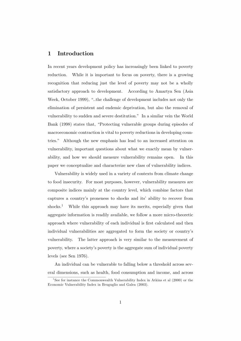
To illustrate our conceptual framework consider two individuals, A and

B, with A having a higher current income relative to B. Suppose the current

income yt, which for simplicity is a proxy for current standard of living, is

positively correlated with the reference line. Let the reference line be a

simple average of the poverty line z, and the current income. Thus for

yt > z, the reference line will lie below the current income and above the

poverty line and for yt < z, then the reference line will lie above the current

income but below the poverty line. Assume that the current income of both6Langarkhanas are soup kitchens which are opened temporarily to feed the famine

stricken.

8

A and B are above the poverty line.

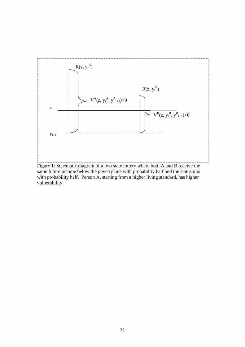
Suppose individuals face the following two state lottery: with probability

half in the �rst state both A and B receive yt+1 < z, and with probability

half in the second state their future income remain the same as the current

income. In the latter state since both receive income equal to their current

income which is above the poverty line, there is no shortfall and will thus

not matter for vulnerability. Therefore, we represent only the �rst state in

a schematic diagram below.

Insert Figure 1

As evident, for both individuals the fall in future income is the same from

the poverty line but di¤erent when considered from their respective current

income. In an expected poverty framework, both A and B would be con-

sidered to be equally vulnerable but in our approach they will have di¤erent

levels of vulnerability. If higher standard of living re�ects a higher reference

line, then as shown in the �gure above, the reference line will be some where

between the poverty line and the current income. Thus the expected fall

from the reference line will be higher for A (shown as V A) than B (shown as

V B), since A has a higher current income. Thus A has higher vulnerability

than B. Note that we consider vulnerability only if future income falls below

the poverty line, otherwise we may end up declaring as vulnerable very rich

individuals whose income might fall below their reference line but still may

be substantially higher than the poverty line or for that matter the income

of most of the population.

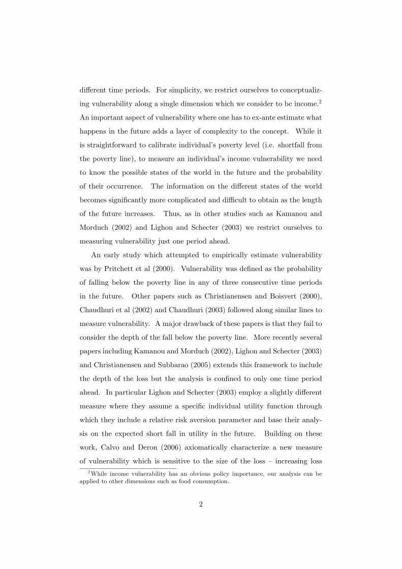
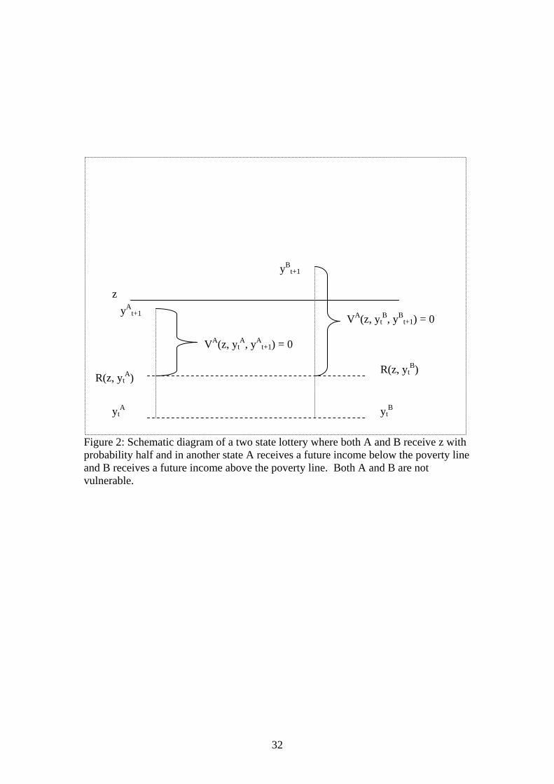
Now let us examine another situation where both individuals have the

same current income but di¤erent future incomes. Consider a two state

lottery with equal probabilities of occurrence where in state 1 both A and

B receive income greater than the poverty line and in state 2 A�s future

income is below the poverty line, while B�s will be above the poverty line.

9

Thus, whatever the state, B will be above the poverty line, whereas A has a

50 percent chance of being poor in the future. As earlier we represent the

state where individuals have a possibility of falling below the poverty line

through the following diagram.

Insert Figure 2

As shown in the �gure above, in state 2 for both individuals their future

incomes are above their reference line. Note that in state 1, both receive an

income above the poverty line and thus would not be deemed vulnerable at

all. In our methodology none of the individuals fall short of their reference

line and hence will not be vulnerable, although clearly one of them has a

high probability to remaining poor in the future. Echoing a similar view

World Bank (1997) state, �The poor are not necessarily vulnerable; for

example, subsistence farmers in remote areas are almost always poor but

are not particularly vulnerable to macroeconomic shocks.� However under

an expected poverty framework, individual A would de�nitely be vulnerable

since he with a positive probability he will remain below the poverty line in

the future. As earlier it is presumed here that the current income and the

reference line are positively correlated. If they were negatively correlated,

however, the reference line would be greater than the poverty line. Thus any

income below the poverty line, would be considered a positive vulnerability.

In the next section we develop these concepts in a formal framework.

2.1 Notation

Suppose an individual faces a �nite set of future incomes fy1t+1; y2t+1; ::; ynt+1g

with probability p = fp1; p2;::; png 2 P where P is the set of probability

distributions such that for all s = 1; ::i; j; ::; n; ps � 0; andnPs=1ps = 1.

Let the poverty line z 2 R++ indicates some minimum income that we

10

expect individuals to have, below which they are considered deprived. Since

our emphasis is on measuring vulnerability of the individual to fall below

poverty, we consider those individuals who have positive probability of falling

below the poverty line z. Thus by avoiding all n-tuple of future incomes

where none of the incomes will be below the given poverty line we will be

focussing only on individuals who has a chance of falling in to poverty in the

future. Individuals whose futute income in all states equal zero are also not

considered. These are the most deprived, but since maximal deprivation is

a certainty vulnerability, which essentially is about the uncertainty in the

future, may not be a relevant issue for such individuals.

We represent the shortfall that the individual faces for each di¤erent

level of future income yst+1 through a deprivation function ds which depends

not only on the level of income in future income yst+1 and the given poverty

line z, but also on an indicator of the standard of living yt 2 R+ of the

individual. Therefore, with any future income yt+1, the associated shortfall

is given by the function d(z; yt; yt+1) where: d : R++�R+�R+ �! R+ and

has the following three properties:

� (P1) d(z; yt; yt+1) 2 R+,

� (P2) d(z; yt; yt+1) is continuous in yt, yt+1, and z, and

� (P3) for �; � > 0 and d(z; yt; yt+1) > 0, d(z+�; yt; yt+1) > d(z; yt; yt+1),

and d(z; yt; yt+1) > d(z; yt; yt+1 + �).

Property (P1) implies that the level of deprivation will not be negative.

The lowest level of deprivation in any state therefore is, zero. Property (P2)

captures the intuition that small changes in yt, yt+1, and z will not lead

to big changes in the level of deprivation. The third property (P3) implies

that if the poverty line z increases the deprivation level will increase too and

if the level of future income yt+1 decreases then vulnerability will decrease.

Note that property P3 holds only when the deprivation is positive.

11

The individual faces a simple deprivation lottery L = (p1; d(z; yt; y1t+1);

:::; pn; d(z; yt; ynt+1)) which is the source of his vulnerability. For notational

convenience ds shall represent d(z; yt; yst+1).

Let F be the set of all deprivation lotteries. Our vulnerability measure

for an individual is a function V : F ! R+. The vulnerability to poverty

depends only on the level of deprivation in each state and the associated

level of probability. A permutation of the states, therefore, will not change

the overall level of vulnerability. In otherwords, it is state independent.

An alternative interpretation, which we will use more extensively, would

be that there are n di¤erent future states of nature and associated with each

state of nature s is an income yst+1 and a deprivation function d(z; yt; yst+1).

The level of income in each of these states re�ect the �nal amount that the

individual receives in the future. So if the individual is unemployed in one

of the future states, then the �nal income that we consider here will take in

to account any insurance that he may have and any bene�ts that he may

receive. Therefore, the coping strategies that individuals may have under

di¤erent states are built in to the �nal income levels.7

One departure from previous axiomatization of measures of vulnerability

is that we do not start with any pre-speci�ed functional form of the depri-

vation function, ds,associated with each state s. The reason is that instead

of comparing the future income in state s from a given benchmark z, we

now also have to take in to consideration the current standard of living yt.

Hence it is not a priori obvious how these three elements will interact to

provide a level of deprivation in each state.

2.2 The Measure

Consider a lottery L = (p1; d(z; yt; y1t+1); p2;d(z; yt; y2t+1); :::; pn; d(z; yt; y

nt+1)).

The general structure of a vulnerability measure V associated with lottery7Coping strategies can also include changing consumption patterns which we do not

consider in this paper.

12

L would be

V (L) =nXs=1

psh�z; yt; y

st+1

�where h is continuous in its arguments.8

However, we can take a step further and untangle the deprivation that

individuals may face in each state of the world. The deprivation in each

state measures the income shortfall in that state from a reference line which

is dependent on both z and yt. Let the shortfall in income in each future

state be: ds(z; yt; yst+1) = R(z; yt)�yst+1; s = 1; ::; n. A class of vulnerability

measures that only considers the level of absolute deprivation in each state

will be bV (L) = nXs=1

psf�R(z; yt)� yst+1

�: (1)

The reference line R(z; yt), re�ects the fact that when it comes to vulnera-

bility the individual considers both his current living standard (represented

here using yt) and also the poverty line as important. It should be noted

that the above equations represents a class of vulnerability measures at the

individual level. To measure the societal vulnerability level one can ag-

gregate the level of vulnerability across all individuals in the society. Our

axiomatization, however, will focus on characterizing a class of measures at

the individual level as represented in (1).

3 Axioms

Our �rst axiom captures the intuition that the vulnerability measure should

be decomposable. In other words, the vulnerability of a convex combination

of lotteries should be the same as the convex combination of the vulnerability

of each of the lotteries. The implication of this axiom would be to make

the vulnerability measure linear in probabilities. It will thus generate the8h can also be considered to re�ect the risk preference of individuals over future income.

13

von Nueman-Morgenstern expected utility structure for the vulnerability

measure.

Axiom 1 Axiom of Decomposability (A1): Consider any two deprivation

lotteries L and L0. Then for 0 � � � 1, V (�L+(1��)L0) = �V (L)+ (1�

�)V (L0) :

As in the case of the von Nueman-Morgenstern expected utility the above

axiom can be derived from more fundamental axioms on the lottery space.

Although this is more of a technical axiom, an intuitive interpretation of the

axiom can be provided along the following lines. Consider the case where

a farmer faces two states (say, normal rainfall and very low rainfall) in the

future but the outcome in those states depends on whether the government

undertakes a policy (such as of providing extra subsidy if it turns out to be

low rainfall and charging higher taxes if it is normal rainfall) which ex-ante

is uncertain. Thus, if the government undertakes the policy the farmer

faces the vulnerability V (L) from lottery L and if it does not then he faces

vulnerability V (L0) from L0. In such case according to Axiom 1 overall

vulnerability should be the �expected�vulnerability. It ignores the fact that

uncertainty in government policy may actually make the overall vulnerability

worse. In this sense the axiom implies that vulnerability is not e¤ected by

higher order uncertainty per se. Broadly what the axiom argues for is that,

if suppose, in the worst case the farmer faces vulnerability V (L0) and in

the best case he faces V (L), then given the uncertainty about whether it is

going to be V (L) or V (L0), it is reasonable to expect that ex-ante overall

vulnerability will be somewhere between V (L) and V (L0). If this is the

case then one natural expectation may be that where exactly between V (L)

and V (L0) the overall vulnerability will lie, should depend on the probability

with which L and L0 takes place. It is this intuition that Axiom 1 captures.

The intuition for our next axiom comes from Sen (1981) who in the

context of Sahelian farmers diversifying in to cash crops notes that although

14

they may have more income, they may be more vulnerable in the sense that

they are more prone to sudden collapse of their entitlement than previously.

Thus in some states of the world the farmers are better o¤ while in other

states they are worse o¤ compared to pre-diversi�cation in to cash crops.

In terms of the distribution it means that although overall the expected

income of the Sahelian farmer may have increased, the expected increase

in inequality between the states outweighs that bene�t and hence leads to

higher vulnerability. A reasonable measure of vulnerability thus should

incorporate the general intuition that as the �distribution�of income becomes

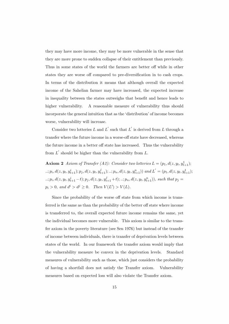
worse, vulnerability will increase.

Consider two lotteries L and L0such that L

0is derived from L through a

transfer where the future income in a worse-o¤ state have decreased, whereas

the future income in a better o¤ state has increased. Thus the vulnerability

from L0should be higher than the vulnerability from L.

Axiom 2 Axiom of Transfer (A2): Consider two lotteries L = (p1; d(z; yt; y1t+1);

::; pi; d(z; yt; yit+1); pj ; d(z; yt; y

jt+1); ::; pn; d(z; yt; y

nt+1)) and L

0= (p1; d(z; yt; y

1t+1);

::; pi; d(z; yt; yit+1� t); pj ; d(z; yt; y

jt+1+ t); ::; pn; d(z; yt; y

nt+1)), such that pj =

pi > 0, and di > dj � 0. Then V (L0) > V (L).

Since the probability of the worse o¤ state from which income is trans-

ferred is the same as than the probability of the better o¤ state where income

is transferred to, the overall expected future income remains the same, yet

the individual becomes more vulnerable. This axiom is similar to the trans-

fer axiom in the poverty literature (see Sen 1976) but instead of the transfer

of income between individuals, there is transfer of deprivation levels between

states of the world. In our framework the transfer axiom would imply that

the vulnerability measure be convex in the deprivation levels. Standard

measures of vulnerability such as those, which just considers the probability

of having a shortfall does not satisfy the Transfer axiom. Vulnerability

measures based on expected loss will also violate the Transfer axiom.

15

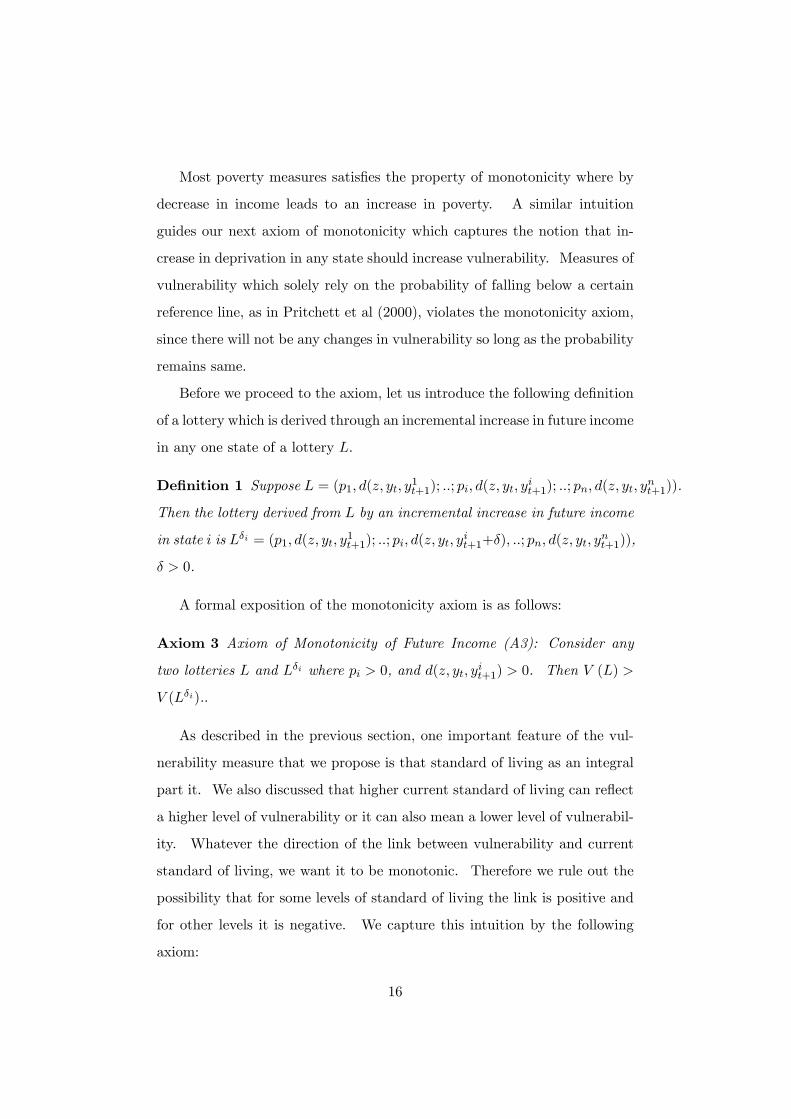
Most poverty measures satis�es the property of monotonicity where by

decrease in income leads to an increase in poverty. A similar intuition

guides our next axiom of monotonicity which captures the notion that in-

crease in deprivation in any state should increase vulnerability. Measures of

vulnerability which solely rely on the probability of falling below a certain

reference line, as in Pritchett et al (2000), violates the monotonicity axiom,

since there will not be any changes in vulnerability so long as the probability

remains same.

Before we proceed to the axiom, let us introduce the following de�nition

of a lottery which is derived through an incremental increase in future income

in any one state of a lottery L.

De�nition 1 Suppose L = (p1; d(z; yt; y1t+1); ::; pi; d(z; yt; yit+1); ::; pn; d(z; yt; y

nt+1)).

Then the lottery derived from L by an incremental increase in future income

in state i is L�i = (p1; d(z; yt; y1t+1); ::; pi; d(z; yt; yit+1+�); ::; pn; d(z; yt; y

nt+1)),

� > 0.

A formal exposition of the monotonicity axiom is as follows:

Axiom 3 Axiom of Monotonicity of Future Income (A3): Consider any

two lotteries L and L�i where pi > 0, and d(z; yt; yit+1) > 0. Then V (L) >

V (L�i).:

As described in the previous section, one important feature of the vul-

nerability measure that we propose is that standard of living as an integral

part it. We also discussed that higher current standard of living can re�ect

a higher level of vulnerability or it can also mean a lower level of vulnerabil-

ity. Whatever the direction of the link between vulnerability and current

standard of living, we want it to be monotonic. Therefore we rule out the

possibility that for some levels of standard of living the link is positive and

for other levels it is negative. We capture this intuition by the following

axiom:

16

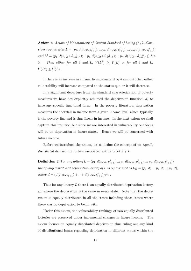
Axiom 4 Axiom of Monotonicity of Current Standard of Living (A4): Con-

sider two lotteries L = (p1; d(z; yt; y1t+1); ::; pi; d(z; yt; yit+1); ::; pn; d(z; yt; y

nt+1))

and L� = (p1; d(z; yt+�; y1t+1); ::; ps; d(z; yt+�; yit+1); ::; pn; d(z; yt+�; y

nt+1)),� >

0. Then either for all � and L, V (L�) � V (L) or for all � and L,

V (L�) � V (L).

If there is an increase in current living standard by � amount, then either

vulnerability will increase compared to the status-quo or it will decrease.

In a signi�cant departure from the standard characterization of poverty

measures we have not explicitly assumed the deprivation function, d, to

have any speci�c functional form. In the poverty literature, deprivation

measures the shortfall in income from a given income level which typically

is the poverty line and is thus linear in income. In the next axiom we shall

capture this intuition but since we are interested in vulnerability our focus

will be on deprivation in future states. Hence we will be concerned with

future income.

Before we introduce the axiom, let us de�ne the concept of an equally

distributed deprivation lottery associated with any lottery L.

De�nition 2 For any lottery L = (p1; d(z; yt; y1t+1); ::; pi; d(z; yt; yit+1); ::; pn; d(z; yt; y

nt+1))

the equally distributed deprivation lottery of L is represented as LE = (p1; d; :::; pk; d; :::; pn; d),

where d = (d(z; yt; y1t+1) + ::+ d(z; yt; ynt+1))=n .

Thus for any lottery L there is an equally distributed deprivation lottery

LE where the deprivation is the same in every state. Note that the depri-

vation is equally distributed in all the states including those states where

there was no deprivation to begin with.

Under this axiom, the vulnerability rankings of two equally distributed

lotteries are preserved under incremental changes in future income. The

axiom focuses on equally distributed deprivation thus ruling out any kind

of distributional issues regarding deprivation in di¤erent states within the

17

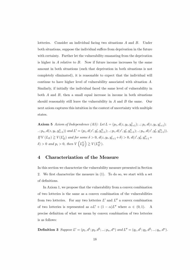
lotteries. Consider an individual facing two situations A and B. Under

both situations, suppose the individual su¤ers from deprivation in the future

with certainty. Further let the vulnerability emanating from the deprivation

is higher in A relative to B. Now if future income increases by the same

amount in both situations (such that deprivation in both situations is not

completely eliminated), it is reasonable to expect that the individual will

continue to have higher level of vulnerability associated with situation A.

Similarly, if initially the individual faced the same level of vulnerability in

both A and B, then a small equal increase in income in both situations

should reasonably still leave the vulnerability in A and B the same. Our

next axiom captures this intuition in the context of uncertainty with multiple

states.

Axiom 5 Axiom of Independence (A5): Let L = (p1; d(z; yt; y1t+1); ::; pi; d(z; yt; yit+1);

::; pn; d(z; yt; ynt+1)) and L

0 = (p1; d(z0; y0t; y01t+1); ::; pi; d(z

0; y0t; y0it+1); ::; pn; d(z

0; y0t; y0nt+1)).

If V (LE) = V (L0E) and for some � > 0, d(z; yt; yit+1+�) > 0, d(z0; y0t; y0it+1+

�) > 0 and pi > 0, then V�L�iE

�= V (L0�iE ).

4 Characterization of the Measure

In this section we characterize the vulnerability measure presented in Section

2. We �rst characterize the measure in (1). To do so, we start with a set

of de�nitions.

In Axiom 1, we propose that the vulnerability from a convex combination

of two lotteries is the same as a convex combination of the vulnerabilities

from two lotteries. For any two lotteries L0 and L00 a convex combination

of two lotteries is represented as �L0 + (1 � �)L00 where � 2 (0; 1). A

precise de�nition of what we mean by convex combination of two lotteries

is as follows:

De�nition 3 Suppose L0 = (p1; d1; p2; d2; :::; pn; dn) and L00 = (q1; d1; q2; d2; :::; qn; dn).

18

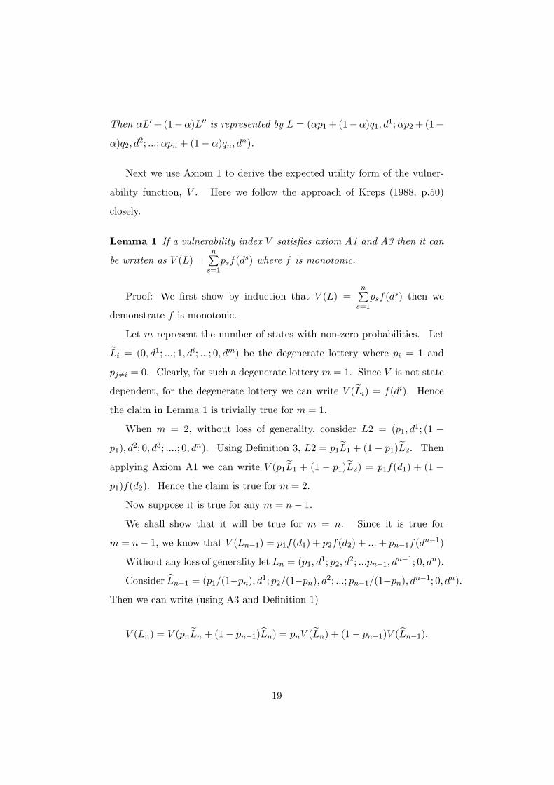
Then �L0+ (1��)L00 is represented by L = (�p1+ (1��)q1; d1;�p2+ (1�

�)q2; d2; :::;�pn + (1� �)qn; dn).

Next we use Axiom 1 to derive the expected utility form of the vulner-

ability function, V . Here we follow the approach of Kreps (1988, p.50)

closely.

Lemma 1 If a vulnerability index V satis�es axiom A1 and A3 then it can

be written as V (L) =nPs=1psf(d

s) where f is monotonic.

Proof: We �rst show by induction that V (L) =nPs=1psf(d

s) then we

demonstrate f is monotonic.

Let m represent the number of states with non-zero probabilities. LeteLi = (0; d1; :::; 1; di; :::; 0; dm) be the degenerate lottery where pi = 1 and

pj 6=i = 0. Clearly, for such a degenerate lottery m = 1: Since V is not state

dependent, for the degenerate lottery we can write V (eLi) = f(di): Hence

the claim in Lemma 1 is trivially true for m = 1:

When m = 2, without loss of generality, consider L2 = (p1; d1; (1 �

p1); d2; 0; d3; ::::; 0; dn). Using De�nition 3, L2 = p1eL1 + (1� p1)eL2. Then

applying Axiom A1 we can write V (p1eL1 + (1 � p1)eL2) = p1f(d1) + (1 �

p1)f(d2). Hence the claim is true for m = 2.

Now suppose it is true for any m = n� 1.

We shall show that it will be true for m = n. Since it is true for

m = n� 1, we know that V (Ln�1) = p1f(d1) + p2f(d2) + :::+ pn�1f(dn�1)

Without any loss of generality let Ln = (p1; d1; p2; d2; :::pn�1; dn�1; 0; dn):

Consider bLn�1 = (p1=(1�pn); d1; p2=(1�pn); d2; :::; pn�1=(1�pn); dn�1; 0; dn).Then we can write (using A3 and De�nition 1)

V (Ln) = V (pneLn + (1� pn�1)bLn) = pnV (eLn) + (1� pn�1)V (bLn�1):

19

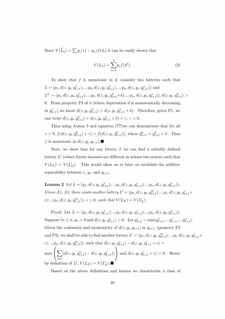
Since V (bLn) =P pi=(1� pn)f(di) it can be easily shown that

V (Ln) =

nXs=1

psf(ds): (2)

To show that f is monotonic in d, consider two lotteries such that

L = (p1; d(z; yt; y1t+1); ::; pk; d(z; yt; y

kt+1); ::; pn; d(z; yt; y

nt+1)) and

L�i = (p1; d(z; yt; y1t+1); ::; pk; d(z; yt; y

kt+1+�); ::; pn; d(z; yt; y

nt+1)), d(z; yt; y

kt+1) >

0. From property P3 of d (where deprivation d is monotonically decreasing

in yst+1) we know d(z; yt; ykt+1) > d(z; yt; y

kt+1 + �). Therefore, given P1, we

can write d(z; yt; ykt+1) = d(z; yt; ykt+1 + �) + , > 0.

Then using Axiom 3 and equation (??)we can demonstrate that for all

> 0, f(d(z; yt; bykt+1) + ) > f(d(z; yt; bykt+1)), where bykt+1 = ykt+1 + �. Thusf is monotonic in d(z; yt; yt+1).�

Next, we show that for any lottery L we can �nd a suitably de�ned

lottery L0 (where future incomes are di¤erent in atleast two states) such that

V (LE) = V (L0E). This would allow us to later on establish the additive

separability between z, yt; and yt+1.

Lemma 2 Let L = (p1; d(z; yt; y1t+1); ::; pi; d(z; yt; yit+1); ::; pn; d(z; yt; y

nt+1)).

Given A1, A3, there exists another lottery L0 = (p1; d(z; yt; y01t+1); ::; pi; d(z; yt; yit+1+

�); ::; pn; d(z; yt; y0nt+1)), � > 0, such that V (LE) = V (L

0E).

Proof: Let L = (p1; d(z; yt; y1t+1); ::; pi; d(z; yt; y

it+1); ::; pn; d(z; yt; y

nt+1)).

Suppose 8s � n; ps > 0 and d(z; yt; yst+1) > 0. Let yit+1 = min(y1t+1; ::; yit+1; ::; ynt+1).

Given the continuity and montonicity of d(z; yt; yt+1) in yt+1, (property P2

and P3), we shall be able to �nd another lottery L0 = (p1; d(z; yt; y01t+1); ::; pi; d(z; yt; yit+1+

�); ::; pn; d(z; yt; y0nt+1)), such that d(z; yt; y

it+1)� d(z; yt; yit+1 + �) =

max

0@Xs 6=i(d(z; yt; y

0st+1)� d(z; yt; yst+1))

1A and d(z; yt; yit+1 + �) > 0. Hence

by de�nition of L0, V (LE) = V (L0E):�

Based on the above de�nitions and lemma we characterize a class of

20

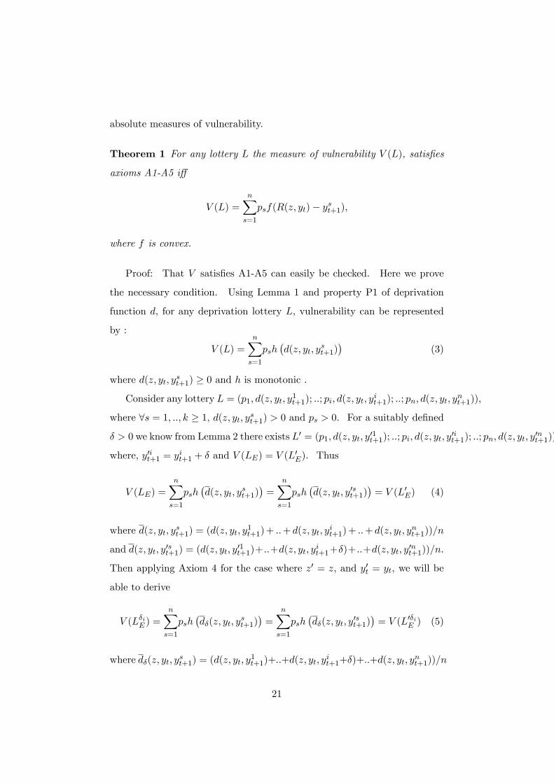
absolute measures of vulnerability.

Theorem 1 For any lottery L the measure of vulnerability V (L), satis�es

axioms A1-A5 i¤

V (L) =

nXs=1

psf(R(z; yt)� yst+1);

where f is convex.

Proof: That V satis�es A1-A5 can easily be checked. Here we prove

the necessary condition. Using Lemma 1 and property P1 of deprivation

function d, for any deprivation lottery L, vulnerability can be represented

by :

V (L) =

nXs=1

psh�d(z; yt; y

st+1)

�(3)

where d(z; yt; yst+1) � 0 and h is monotonic .

Consider any lottery L = (p1; d(z; yt; y1t+1); ::; pi; d(z; yt; yit+1); ::; pn; d(z; yt; y

nt+1)),

where 8s = 1; ::; k � 1, d(z; yt; yst+1) > 0 and ps > 0. For a suitably de�ned

� > 0 we know from Lemma 2 there exists L0 = (p1; d(z; yt; y01t+1); ::; pi; d(z; yt; y0it+1); ::; pn; d(z; yt; y

0nt+1))

where; y0it+1 = yit+1 + � and V (LE) = V (L

0E). Thus

V (LE) =

nXs=1

psh�d(z; yt; y

st+1)

�=

nXs=1

psh�d(z; yt; y

0st+1)

�= V (L0E) (4)

where d(z; yt; yst+1) = (d(z; yt; y1t+1)+ ::+ d(z; yt; y

it+1)+ ::+ d(z; yt; y

nt+1))=n

and d(z; yt; y0st+1) = (d(z; yt; y01t+1)+::+d(z; yt; y

it+1+�)+::+d(z; yt; y

0nt+1))=n.

Then applying Axiom 4 for the case where z0 = z; and y0t = yt, we will be

able to derive

V (L�iE ) =

nXs=1

psh�d�(z; yt; y

st+1)

�=

nXs=1

psh�d�(z; yt; y

0st+1)

�= V (L0�iE ) (5)

where d�(z; yt; yst+1) = (d(z; yt; y1t+1)+::+d(z; yt; y

it+1+�)+::+d(z; yt; y

nt+1))=n

21

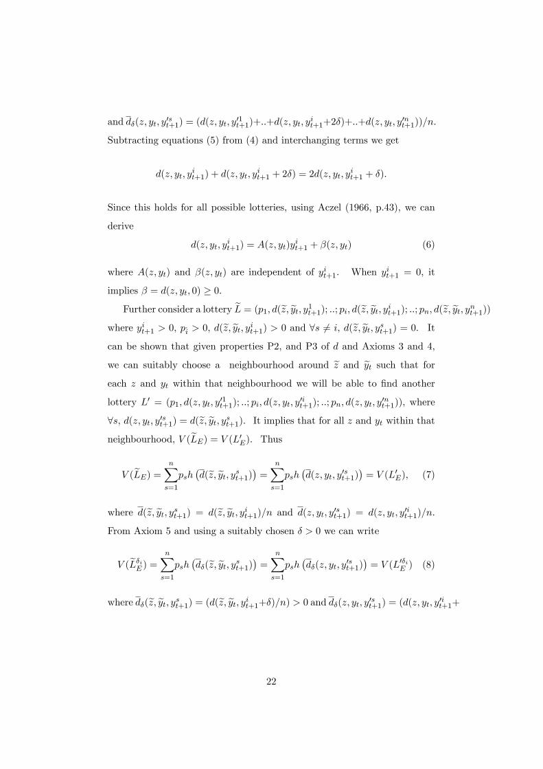
and d�(z; yt; y0st+1) = (d(z; yt; y01t+1)+::+d(z; yt; y

it+1+2�)+::+d(z; yt; y

0nt+1))=n.

Subtracting equations (5) from (4) and interchanging terms we get

d(z; yt; yit+1) + d(z; yt; y

it+1 + 2�) = 2d(z; yt; y

it+1 + �):

Since this holds for all possible lotteries, using Aczel (1966, p.43), we can

derive

d(z; yt; yit+1) = A(z; yt)y

it+1 + �(z; yt) (6)

where A(z; yt) and �(z; yt) are independent of yit+1. When yit+1 = 0, it

implies � = d(z; yt; 0) � 0.

Further consider a lottery eL = (p1; d(ez; eyt; y1t+1); ::; pi; d(ez; eyt; yit+1); ::; pn; d(ez; eyt; ynt+1))where yit+1 > 0, p_i > 0, d(ez; eyt; yit+1) > 0 and 8s 6= i, d(ez; eyt; yst+1) = 0. It

can be shown that given properties P2, and P3 of d and Axioms 3 and 4,

we can suitably choose a neighbourhood around ez and eyt such that foreach z and yt within that neighbourhood we will be able to �nd another

lottery L0 = (p1; d(z; yt; y01t+1); ::; pi; d(z; yt; y

0it+1); ::; pn; d(z; yt; y

0nt+1)), where

8s, d(z; yt; y0st+1) = d(ez; eyt; yst+1). It implies that for all z and yt within thatneighbourhood, V (eLE) = V (L0E). ThusV (eLE) = nX

s=1

psh�d(ez; eyt; yst+1)� = nX

s=1

psh�d(z; yt; y

0st+1)

�= V (L0E); (7)

where d(ez; eyt; yst+1) = d(ez; eyt; yit+1)=n and d(z; yt; y0st+1) = d(z; yt; y0it+1)=n.

From Axiom 5 and using a suitably chosen � > 0 we can write

V (eL�iE ) = nXs=1

psh�d�(ez; eyt; yst+1)� = nX

s=1

psh�d�(z; yt; y

0st+1)

�= V (L0�iE ) (8)

where d�(ez; eyt; yst+1) = (d(ez; eyt; yit+1+�)=n) > 0 and d�(z; yt; y0st+1) = (d(z; yt; y0it+1+

22

�)=n) > 0. Subtracting (7) from (8) and using (6), we can show

A(ez; eyt) = A(z; yt):Since this must hold for all values of z and yt within the suitably de�ned

neighbourhood, it can only be true if A(z; yt) = A(z; yt) = w, where w is a

constant. Thus

d(z; yt; yit+1) = wy

it+1 + �(z; yt) (9)

Next consider any lottery L and the associated lottery L�i , where pi > 0.

Using axiom A3 and (9) one can show w < 0. Further d(z; yt; yit+1) 2 R+(from property P1 of d(z; yt; yit+1)). Thus (6) can be written as

d(z; yt; yit+1) =

8<: �(R(z; yt)� yit+1) if R(z; yt) � yit+10 otherwise

; (10)

where R(z; yt) = (�(z; yt)=�) and � = jwj.

We next demonstrate that h is convex. Consider two lotteries L =

(p1; d(z; yt; y1t+1); ::; pi; d(z; yt; y

it+1); pj ; d(z; yt; y

jt+1); ::; pn; d(z; yt; y

nt+1)) and

L0= (p1; d(z; yt; y

1t+1); ::; pi; d(z; yt; y

it+1�t); pj ; d(z; yt; y

jt+1+t); ::; pn; d(z; yt; y

nt+1))

where pj = pi > 0, and d(z; yt; yit+1) > d(z; yt; yjt+1) > 0. Using axiom A2,

(3) and cancelling terms we get

((h(d(z; yt; yit+1�t))�h(d(z; yt; yit+1)) > h(d(z; yt; y

jt+1))�h(d(z; yt; y

jt+1+t))

Using (10), from the above equation one can derive

(h(di(z; yt; yit+1)+�)�h(di(z; yt; yit+1)) > h(dj(z; yt; y

jt+1))�h(dj(z; yt; y

jt+1)��)

(11)

where � = �t. Thus h is a convex function of the deprivation level, d

(Royden 1988).

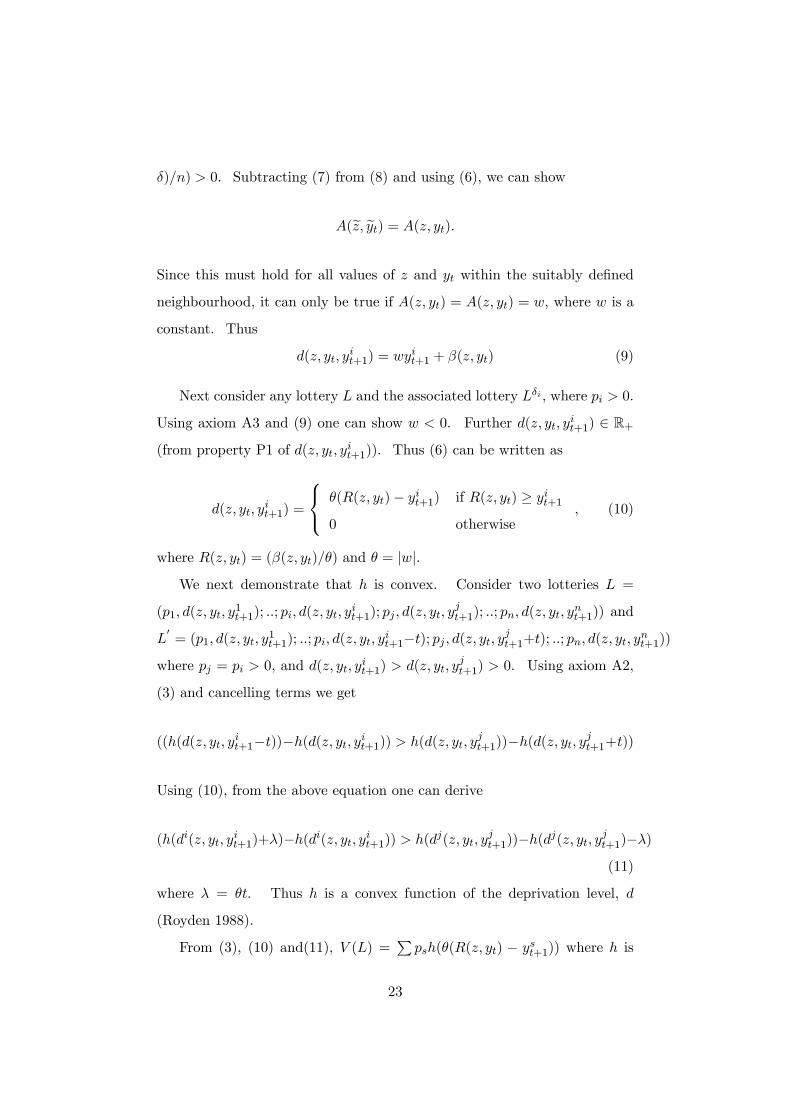
From (3), (10) and(11), V (L) =Ppsh(�(R(z; yt) � yst+1)) where h is

23

convex. Since � > 0 is a constant, we can write V (L) =Ppsf(R(z; yt) �

yst+1), where f is convex. �

5 Discussion

So far we have characterized a broad class of vulnerability measure. How-

ever, for empirical applications speci�c functional forms are required, which

we shall elaborate on in this section. In (1) both the reference income

R(z; yt), and vulnerability under a degenerate lottery, represented by f ,

have general structures that can be made more speci�c.

There are several functional forms that can be used for representing

R(z; yt) depending on how z and yt are related and whether yt is positively

or negatively correlated with R(z; yt). One interpretation of R(z; yt) is that

it is the minimum living standard that people should maintain in the future

to be not considered as vulnerable. It is, however, quite reasonable to expect

that for every doubling of the current income, the minimum living standard

R(z; yt) will not double too. In other words, reasonable R(z; yt) should

satisfy the condition that changes in current income does not translate to

equivalent changes in the reference line.

If yt and R(z; yt) are positively correlated, an interesting functional form

of the reference line is R(z; yt) = z1��y�t where 0 � � � 1 (see Foster 1998).

It is homogenous of degree 1 (HD-1) and satis�es the property that a percent

change in yt leads to a � � 1 percent change in R(z; yt). This implies that

the current income elasticity of the reference line is not greater than one

which concurs with our intuition that reference income should not vary too

much with changes in current income. Another functional representation of

the reference line is R(z; yt) = (1� �)z + �yt where 0 � � � 1. Clearly the

rate of change in reference income with respect to the current income is less

than one. So long as (1 � �)=� > z=yt, it is also the case that the current

income elasticity of the reference line is less or equal to one.

24

On the other hand if yt and R(z; yt) are negatively correlated, the ref-

erence line can be represented by R(z; yt) = z1+�=y�t where 0 � � � 1.

Clearly as yt increases, R(z; yt) decreases indicating that a currently richer

person would su¤er less vulnerability compared a poorer person for same

level of future income. Here again the absolute current income elasticity of

the reference line is less than one. The linear representation of the reference

line is R(z; yt) = (1 � �)z � �yt where 0 � � � 1. Under this functional

form, with su¢ ciently high yt it is possible to generate R(z; yt) < 0, which

implies that those with high levels of income in the current period would

not be vulnerable what ever their future income is.

Given a particular functional form of the reference line and depending on

the choice of f , speci�c classes of measures of vulnerability can be derived.

For example, we can generate the Foster-Greer-Thorbecke (FGT) class of

absolute vulnerability measures which is

V (L) =nXs=1

ps�Az1��y�t � yst+1

� (12)

where > 1. Note that if � 1, then the vulnerability function for each

state of the world will not be convex thus violating axiom A2. When � = 0,

the measure would be the standard expected FGT poverty index. When

� = 1, the measure is completely relative in the sense that it depends on the

current and future income. Thus by varying � we can get a whole set of

values of vulnerability ranging from the expected poverty measures to the

relative measures. From this perspective, the class of measure that we have

proposed is very general and incorporates the expected poverty measures as

a special case.

25

6 Conclusion

In this paper we have attempted to conceptualize and characterize a new

class of vulnerability measure. Detailed case studies indicate that existing

measures of vulnerability based on the expected poverty framework may be

unable to fully capture the di¤erent facets of vulnerability. The studies

also �nd that individual�s current levels of wealth and income impact their

income vulnerability by a¤ecting their ability to build up coping mechanisms

for future income shocks and also by their willingness to use current levels

of income and wealth as benchmarks for the future living standards. Our

proposed measure, by taking into account current assets and income, is

thus closer to the broader notion of vulnerability. It has to be noted that

although our exposition of the measure in this paper is based on income,

it can be applied for calibrating vulnerability along other dimensions of

well-being. Thus if we are interested in food insecurity, we can use food

consumption instead of income and arrive at a measure of vulnerability to

food deprivation.

We use the standard framework of decision making under uncertainty to

characterize a class of absolute measure of vulnerability. The measure that

we have characterized extremely general. For instance the functional form

of our reference line which combines the poverty line and some indicator

of the living standard (such as income) is left quite unrestricted. Thus,

unlike other measures we are able to consider two opposing view points: (a)

where current living standard reduces future vulnerability and (b) where

current living standards exacerbates future vulnerability, within one uni�ed

framework. We also provide speci�c examples of our measure by indicating

how the FGT indices can be adopted for our measures. Despite the gen-

erality, our axioms rule out some obvious measures of vulnerability such as

those belonging to FGT class of vulnerability measures (12) with = 0,1.

Although we have provided an example of our measure, depending on func-

26

tional structures many more vulnerability measures can be developed.

There are, however, some shortcomings in our analysis. In particular we

have considered vulnerability just one period ahead. Although analyzing

vulnerability too far in the future may be meaningless, vulnerability over

multiple time periods would considerably enrich the analysis. We have also

assumed a probability distribution over future states of the world. But in

a completely uncertain world we may not have those information and thus

may not be able to apply the standard von-Nueman Morgenstern framework.

Finally it is quite probable that some speci�c measures of the proposed class

of measures may not always satisfy reasonable properties. For instance

Menezes et al (1980) considers a downward shift of a distribution, keeping

the mean and the variance the same, as re�ecting higher down side risk and

thus higher vulnerability. It can, however, be easily shown that the FGT

class (12) for = 2 does not satisfy the property of higher vulnerability

emanating from a downward movement of the distribution. What would

be the most parsimonious structure that will capture all the di¤erent facets

of vulnerability remains a topic of further research.

27

References

Atkins, J. P., S. Mazzi and C.D. Easter (2000), A Commonwealth Vulner-

ability Index for Developing Countries: The Position of Small States,

Economic Paper 40, Common Wealth Secretariat.

Basu, K. and P. Nolen (2005), Vulnerability, Unemployment and Poverty:

A New Class of Measures, Its Axiomatic Properties and Applications,

Mimeo.

Bruguglio, L. and W. Galea (2003). Updating and Augmenting the Eco-

nomic Vulnerability Index. Occasional paper, University of Malta.

Calvo, C. and S. Dercon (2006), Measuring Individual Vulnerability, Mimeo.

Chaudhuri, S., J. Jalan and A. Suryahadi (2002), Assessing Household

Vulnerability to Poverty from Cross-Sectional Data: A Methodology

and Estimates from Indonesia, Working Paper, Columbia University.

Chaudhuri, S. (2003), Assessing Vulnerability to Poverty: Concepts, Em-

pirical Methods and Illustrative Examples,Working Paper, Columbia

University.

Christianensen, L. and R. N. Boisvert (2000) On Measuring Household

Food Vulnerability: Case Evidence from Nothern Mali, Working Pa-

per, World Bank.

Dercon, S. and P. Krishnan (2000), In Sickness and In Health: Risk Sharing

within Households in Rural Ethiopia, Journal of Political Economy,

108, 688-727.

Evanson, E. (1985), On the Edge: A study of Poverty and Long term

Unemployment in Northern Ireland, Child Poverty Action Group.

Ersado, L. (2008), Rural Vulnerability in Serbia, Working Paper 4010,

World Bank.

28

Foster, J (1998), Absolute versus Relative Poverty, American Economic

Review Papers and Proceedings, 88, 335-341.

Hoddinott, J. and A. Quisumbing (2003), Methods of Microeconometric

Risk and Vulnerability Assessments, SPDP Series 0324, World Bank

Kamanou, G., and J. Morduch (2002) Measuring Vulnerability to Poverty,

WIDER Discussion Paper, 2002/58

Kreps, D. (1988), Notes on the Theory of Choice, Westview Press, Boulder.

Ligon, E. and L. Schecter (2003), Measuring Vulnerability, Economic Jour-

nal, 113, C95-C102.

Menezes, C., C. Geiss and J. Tressler (1980), Increasing Downside Risk,

American Economic Review, 921-932.

Morduch, J. (1994), Poverty and Vulnerability, American Economic Review

Papers and Proceedings, 84, 221-225.

Moser, C. O. N. (1996) Confronting Crisis: A Comparative Study of House-

holds Response to Poverty and Vulnerability in Four Poor Urbane

Communities, Working Paper, ESD No. 8, World Bank.

Niculescu, C.P. and L-E, Persson (2006) Convex Functions and Their Ap-

plications: A Contemporary Approach, Springer, New York.

Pritchett, L., A. Suryahadi and S. Sumarto (2000), Quantifying Vulnera-

bility to Poverty, World Bank, Policy Research Working Paper 2437.

Royden, H. L. (1988), Real Analysis: 3rd Edition, McMillan, US.

Sen, A. (1976), Poverty: An Ordinal Approach to Measurement, Econo-

metrica, 44, 219-231.

Sen, A (1981), Poverty and Famines, Oxford University Press, Oxford.

29

Sen, A. (1999), A Plan for Asia�s Growth, Asia Week, October 8, 25. Avail-

able at: http://www.asiaweek.com/asiaweek/magazine/99/1008/viewpoint.html

Simon, C. P. and L. Blume, (1994), Mathematics for Economists, W.W.Norton

& Co., London

World Bank (1997), Poverty Lines, Policy Research and Poverty and Social

Policy DepartmentWorld Bank, No. 6. Available at http://www.worldbank.org/html/

prdph/lsms/research/povline/pl_n06.pdf.

30

31

Figure 1: Schematic diagram of a two state lottery where both A and B receive the same future income below the poverty line with probability half and the status quo with probability half. Person A, starting from a higher living standard, has higher vulnerability.

z

R(z, ytB)

R(z, ytA)

VA(z, ytA, yA

t+1)>0

yt+1

VB(z, ytB, yB

t+1)>0

32

Figure 2: Schematic diagram of a two state lottery where both A and B receive z with probability half and in another state A receives a future income below the poverty line and B receives a future income above the poverty line. Both A and B are not vulnerable.

z

R(z, ytB)

R(z, ytA)

VA(z, ytA, yA

t+1) = 0

yAt+1 VA(z, yt

B, yBt+1) = 0

yBt+1

ytB

ytA