on of Two-Dimensional Skeletonization Algorithms - IEEE

8/2/2019 on of Two-Dimensional Skeletonization Algorithms - IEEE

http://slidepdf.com/reader/full/on-of-two-dimensional-skeletonization-algorithms-ieee 1/23

1

Parallelization of Two‐Dimensional Skeletonization Algorithms

Bhavya Daya

Electrical &

Computer

Engineering

Department,

University

of

Florida

Abstract

Non‐ pixel based skeletonization techniques have advantages over traditional pixel ‐based method, such as distance

transform and thinning. One of the advantages includes a faster processing time. The disadvantage of non‐ pixel based

techniques is the complexity. Pixel ‐based techniques are easier to implement and computational efficiency can be achieved by

taking advantage of parallel computers. The parallelization of the pixel ‐based techniques, thinning and distance transform, is

formulated, designed, compared and optimized. One algorithm, the distance transform, proved superior in performance and

quality of skeletonization. It was showed that the serial and parallel distance transform algorithm performs better than the serial

and

parallel

thinning

algorithm.

Results

showed

that

the

proposed

parallel

algorithm

is

computationally

efficient

and

closely

aligns with the human’s perception of the underlying shape. Optimizations were performed without compromising the quality of

the skeletonization.

Many applications depend on the skeletonization algorithm. The parallelization of the skeletonization algorithm creates

a stepping stone for the entire image processing application to enter the parallel computing realm. Increasing the performance

of the skeletonization process will speed up the applications that depend on the algorithm.

1. Introduction

Image skeletonization is one of the many morphological image processing operations. By combining different

morphological image

processing

applications,

an

algorithm

can

be

obtained

for

many

image

processing

tasks,

such

as

feature

detection, image segmentation, image sharpening, and image filtering. Image skeletonization is especially suited to the

processing of binary images or grayscale images. The parallelization of the skeletonization algorithm will provide a stepping

stone for image processing applications to transcend to the parallel computing realm. Many sequential algorithms exist for

achieving a two‐dimensional binary image skeletonization.

For a skeleton of an image to be successful and useful in its designated application, it must possess three properties [1]:

1. It must be closely aligned with the human’s perception of the underlying shape

2. It must be robust against noise

3. It must be computed in an efficient and timely manner

Skeletonization is achieved by two common methods, thinning and distance transform. Thinning and distance

transform are pixel based techniques that need to process every pixel in the image [1]. This can incur a long processing time and

leads to reduced efficiency. Various techniques have been developed and implemented, but a large percentage of them possess

some common faults that limit their use. These faults include noise sensitivity, excessive processing time, and results not

conforming to a human’s perception of the underlying object in the image [1]. Since skeletonization is very often an

intermediate step towards object recognition, it should have a low computation cost.



2

2. Related Work

The literature survey unveiled that many different skeletonization algorithms are performed to obtain the three main

goals of a good algorithm. Some algorithms emphasize one goal more than another.

The connectivity of the image is also greatly considered in skeletonization algorithms. Many perform variations of the

distance transform

and

thinning

approaches.

Some

even

attempted

a hybrid

form

of

the

two.

[8]

Since

skeletonization

works

well when it is tailored for particular images, many algorithms were devised to obtain the skeletons of these specific image

types. The major problem of the algorithms is that it works well for some images and not others, especially with regard to

thinning algorithms.

Some complex techniques that have been developed that aren’t pixel‐based techniques. These techniques conform to

the skeleton requirements and are computed efficiently. [1] The parallelization of these algorithms would seem useless due to

its efficiency. A simple algorithm can achieve the performance on a parallel computer comparable or even better than a

complex algorithm on a sequential machine.

Some literature mentions that the transitioning of two‐dimensional skeletonization to three‐dimensional

skeletonization is a difficult process. The 3D skeletonization techniques were surveyed, most of them start off using the two‐

dimensional techniques of thinning or distance transform. [3]

3. Background

The generation of a digital image skeleton is often one of the first processing steps taken by a computer vision system

when attempting to extract features from an object in an image. Due to its compact shape representations, image

skeletonization has been studied for a long time in computer vision, pattern recognition and Optical Character Recognition. It is

a powerful tool for intermediate representation for a number of geometric operations on solid models.

An image skeleton is presumed to represent the shape of the object in a relatively small number of pixels, all of which

are, in some sense, structural and therefore necessary. The skeleton of an object is, conceptually, defined as the locus of center

pixels in the object. [3] Unfortunately, no generally agreed upon definition of a digital image skeleton exists. Of the literally

hundreds of

papers

on

the

subject

of

thinning

which

are

in

print,

the

vast

majority

are

concerned

with

the

implementation

of

a

variation on an existing thinning method, where the novel aspects are related to the performance of the algorithm. But for all

definitions, at least 4 requirements below must be satisfied for skeleton objects [3]:

1. Centeredness satisfaction: Skeleton is geometrically centered within the object boundary or as close as possible.

2. Connectivity preservation: The output skeleton should have the same connectivity as the original object and

should not contain any background element.

3. Topology must remain constant

4. As thin as possible: 1‐pixel thin is the requirement for a 2D skeleton, and in 3D, as thin as possible.

Although the

target

is

to

satisfy

the

skeleton

requirements,

many

algorithms

perform

well

on

certain

types

of

images.

Some algorithms provide an excellent skeleton for one image and a horrible one for another image. An algorithm should be fast

and reliable in producing a good skeleton on any image. The quality is just as important as the execution time of the algorithm.

The simplest type of image which is used widely in a variety of industrial and medical applications is binary, i.e. a black‐

and‐white or silhouette image. [4] A binary image is usually stored in memory as a bitmap, a packed array of bits. Binary image

processing has several advantages but some corresponding drawbacks:



3

Table 1: Advantages and Disadvantages of Binary Images

Advantages

• Easy to acquire

• Low storage: no more than 1 bit/pixel, often this can be reduced as such images are

very amenable to compression.

• Simple processing

Disadvantages

• Limited application: as the representation is only a silhouette, application is

restricted to tasks where internal detail is not required as a distinguishing

characteristic.

• Specialized

lighting

is

required

for

silhouettes:

it

is

difficult

to

obtain

reliable

binary

images without restricting the environment.

There are different categories of skeletonization methods: one category is based on distance transforms, and a

specified subset of the transformed image is a distance skeleton. [1] Another category is defined by thinning approaches; and

the result of skeletonization using thinning algorithms should be a connected set of digital curves or arcs. [1] Thinning

algorithms are a very active area of research, with a main focus on connectivity preserving methods allowing parallel

implementation. Images below display the results of a 2D skeletonization thinning algorithm.

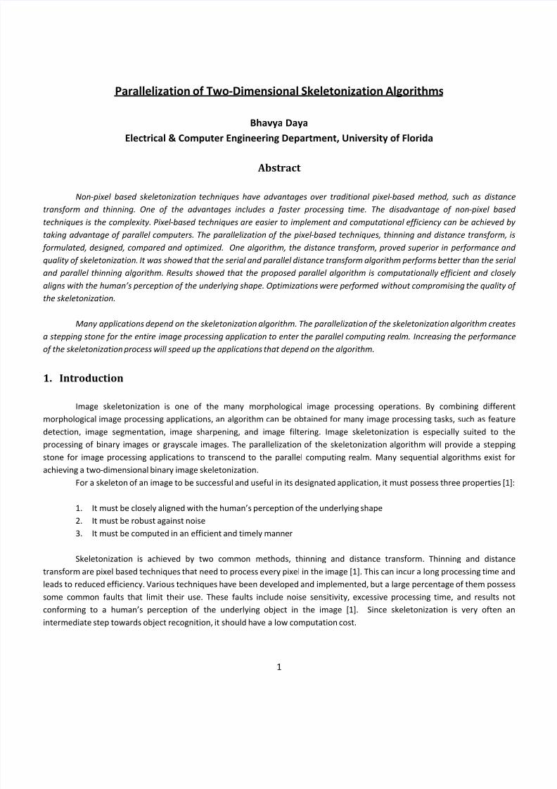
Thinning or erosion of the image is a method that iteratively peels off the boundary layer by layer from outside to

inside. The removal does not affect the topology of the image. This is a repetitive and time‐consuming process of testing and

deletion of each pixel. It is good for connectivity preservation. The problem with this approach is that the set of rules defining

the removal of a pixel is highly dependent on the type of image and different set of rules will be applied for different types of

images. Figure 4 is an image of the thinning process as applied to a three‐dimensional image. The phases are the thinning layers.

Figure 2: Intermediate Step [3] Figure 3: Skeleton of Original Image [3] Figure 1: Original Image [3]



4

Figure 4: Thinning applied to 3D image [5]

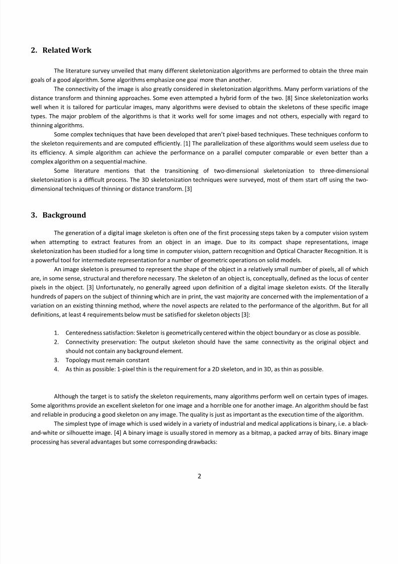
The distance transform is the other common technique for achieving the medial axis or skeleton of the image. There

are three main types of distance transforms, chamfer based, Euclidean and voronoi diagram based. [5] The simplest approach

for the skeletonization algorithm is the Euclidean distance transform. This method is based on the distance of each pixel to the

boundary and tries to extract the skeleton by finding the pixels in the center of the object; these pixels are the furthest from the

boundary. The distance coding is based on the Euclidean distance. This method is faster than the thinning approach and can be

done in high degree of parallelism. [1] Unfortunately, the output is not guaranteed to preserve connectivity. The distance

transform process applied to skeletonization can be visualized as in the figure below. The ridges on the image to the right

belong to the skeleton.

As mentioned earlier, the computation cost of these methods affects the use of the skeletonization algorithm.

Skeletonization is an essential part of image processing applications, with the increase in performance of skeletonization

techniques the applications will also have a lower computation cost.

4. Methodology The serial code for both algorithms was written for comparison with parallel algorithms. In order to determine if the

serial code was achieving a skeletonization that was appropriate, it was compared to MATLAB’s results for the skeletonization.

MATLAB contains

the

functionality

to

perform

the

distance

transform

skeletonization

process

and

the

thinning

skeletonization

process. MATLAB uses a different algorithm for performing the thinning skeletonization process and uses a different distance

transform for achieving skeletonization. The distance transform skeletonization process implemented in MATLAB achieves the

skeletonization by performing the Euclidean Distance Transform.

A shared memory architecture, Marvel Cluster, was chosen for implementation. The machine contains 16 symmetric

multiprocessors with 32 GB of memory. Both algorithms use the domain decomposition approach. The image matrix is stored in

shared memory for access by any processor. Each processor contains in local memory a piece of the entire image matrix that is

Figure 5: Original

Image [5] Figure 6: Distance

Transform [5]



5

relevant for its calculations. If other matrix values is not present in local memory and is required, the value is fetched from

shared memory.

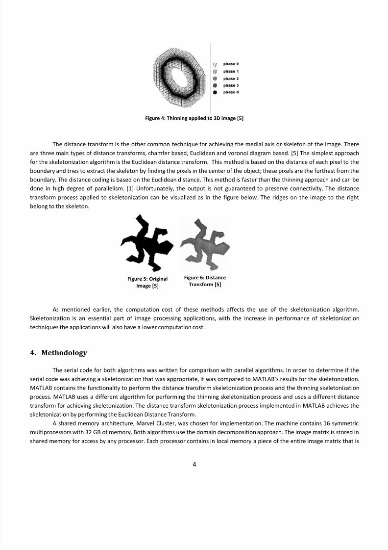
The image is statically allocated by dividing the image into strips. Each processor or thread is assigned to perform

computation on the strip that is allocated to it. Each processor performs the same computation on different sets of data or in

this case, different parts of the image matrix. The split allocation is shown in the image below.

Figure 7:

Thread

Allocation

The shared memory machine was chosen for this application for a couple main reasons. Before these reasons are

mentioned, it is useful to consider why clusters and a message passing machine were not utilized. Message passing machines

have proven in the past that performance obtained is greater than shared memory machines. Since there are a lot of data that

requires processing and the communication between processors without shared memory is predicted to be quite large, the

shared memory communication abstraction was chosen. The shared memory machine was predicted to perform well when the

application requires data decomposition and large amount of data.

4.1 Parallelization of

Distance

Transform

Algorithm

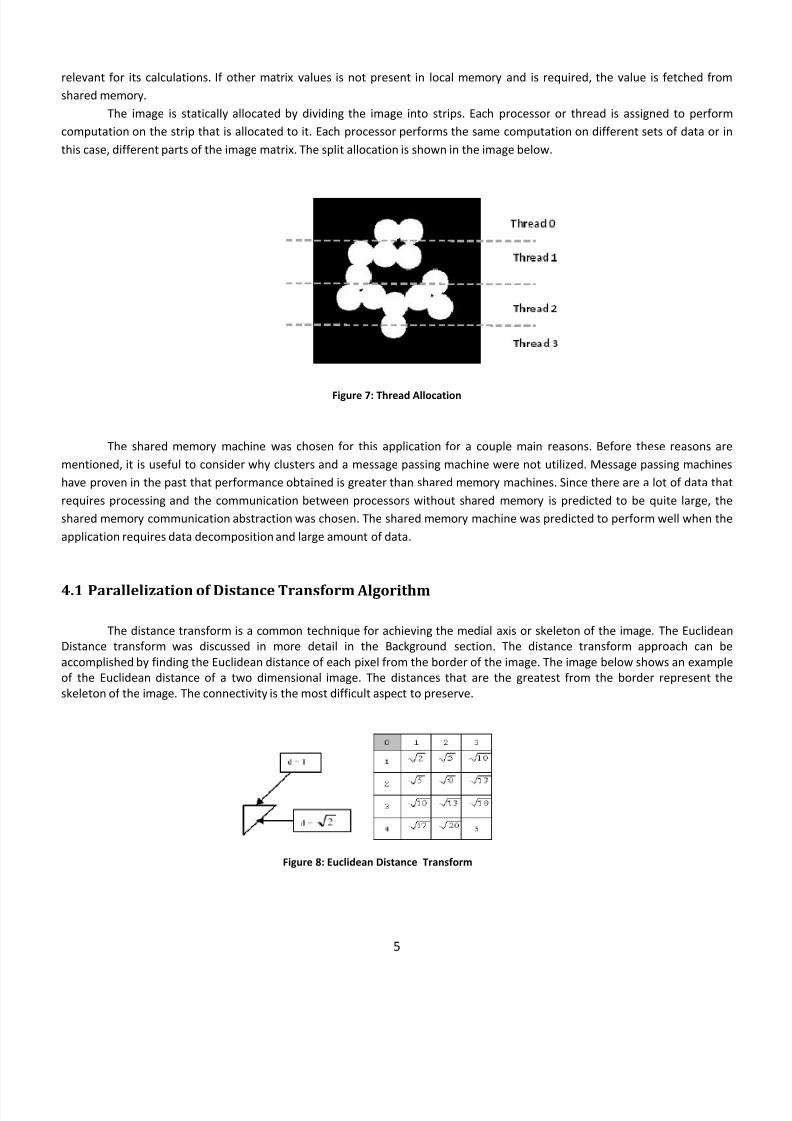
The distance transform is a common technique for achieving the medial axis or skeleton of the image. The Euclidean

Distance transform was discussed in more detail in the Background section. The distance transform approach can be

accomplished by finding the Euclidean distance of each pixel from the border of the image. The image below shows an example

of the Euclidean distance of a two dimensional image. The distances that are the greatest from the border represent the

skeleton of the image. The connectivity is the most difficult aspect to preserve.

Figure 8: Euclidean Distance Transform



6

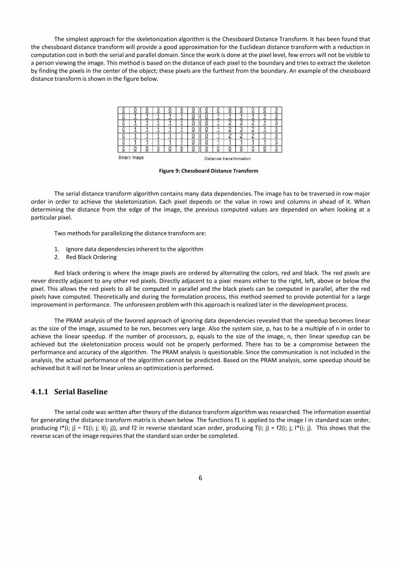
The simplest approach for the skeletonization algorithm is the Chessboard Distance Transform. It has been found that

the chessboard distance transform will provide a good approximation for the Euclidean distance transform with a reduction in

computation cost in both the serial and parallel domain. Since the work is done at the pixel level, few errors will not be visible to

a person viewing the image. This method is based on the distance of each pixel to the boundary and tries to extract the skeleton

by finding the pixels in the center of the object; these pixels are the furthest from the boundary. An example of the chessboard

distance transform is shown in the figure below.

The serial distance transform algorithm contains many data dependencies. The image has to be traversed in row major

order

in

order

to

achieve

the

skeletonization.

Each

pixel

depends

on

the

value

in

rows

and

columns

in

ahead

of

it.

When

determining the distance from the edge of the image, the previous computed values are depended on when looking at a

particular pixel.

Two methods for parallelizing the distance transform are:

1. Ignore data dependencies inherent to the algorithm

2. Red Black Ordering

Red black ordering is where the image pixels are ordered by alternating the colors, red and black. The red pixels are

never directly adjacent to any other red pixels. Directly adjacent to a pixel means either to the right, left, above or below the

pixel. This allows the red pixels to all be computed in parallel and the black pixels can be computed in parallel, after the red

pixels have

computed.

Theoretically

and

during

the

formulation

process,

this

method

seemed

to

provide

potential

for

a large

improvement in performance. The unforeseen problem with this approach is realized later in the development process.

The PRAM analysis of the favored approach of ignoring data dependencies revealed that the speedup becomes linear

as the size of the image, assumed to be nxn, becomes very large. Also the system size, p, has to be a multiple of n in order to

achieve the linear speedup. If the number of processors, p, equals to the size of the image, n, then linear speedup can be

achieved but the skeletonization process would not be properly performed. There has to be a compromise between the

performance and accuracy of the algorithm. The PRAM analysis is questionable. Since the communication is not included in the

analysis, the actual performance of the algorithm cannot be predicted. Based on the PRAM analysis, some speedup should be

achieved but it will not be linear unless an optimization is performed.

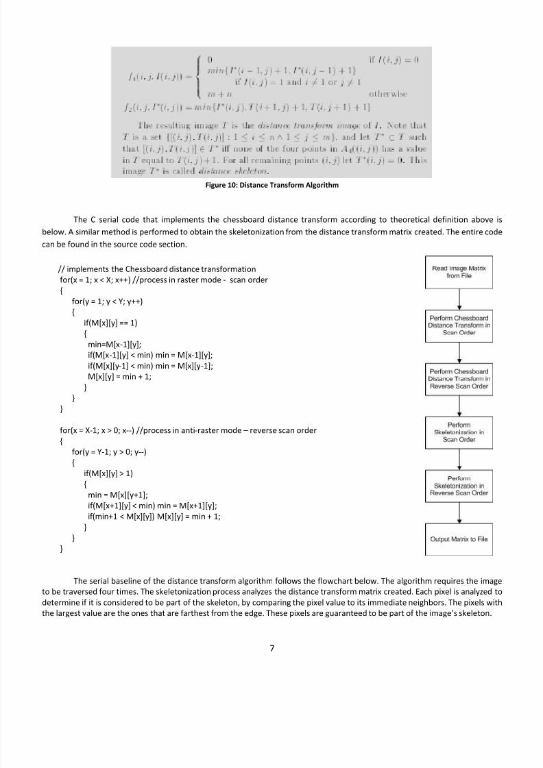
4.1.1 Serial Baseline The serial code was written after theory of the distance transform algorithm was researched. The information essential

for generating the distance transform matrix is shown below. The functions f1 is applied to the image I in standard scan order,

producing I*(i; j) = f1(i; j; I(i; j)), and f2 in reverse standard scan order, producing T(i; j) = f2(i; j; I*(i; j). This shows that the

reverse scan of the image requires that the standard scan order be completed.

Figure 9: Chessboard Distance Transform



7

Figure 10: Distance Transform Algorithm

The C serial code that implements the chessboard distance transform according to theoretical definition above is

below. A similar method is performed to obtain the skeletonization from the distance transform matrix created. The entire code

can be found in the source code section.

// implements

the

Chessboard

distance

transformation

for(x = 1; x < X; x++) //process in raster mode ‐ scan order

{

for(y = 1; y < Y; y++)

{

if(M[x][y] == 1)

{

min=M[x‐1][y];

if(M[x‐1][y] < min) min = M[x‐1][y];

if(M[x][y‐1] < min) min = M[x][y‐1];

M[x][y] = min + 1;

}

}

}

for(x = X‐1; x > 0; x‐‐) //process in anti‐raster mode – reverse scan order

{

for(y = Y‐1; y > 0; y‐‐)

{

if(M[x][y] > 1)

{

min = M[x][y+1];

if(M[x+1][y] < min) min = M[x+1][y];

if(min+1 < M[x][y]) M[x][y] = min + 1;

}

}

}

The serial baseline of the distance transform algorithm follows the flowchart below. The algorithm requires the image

to be traversed four times. The skeletonization process analyzes the distance transform matrix created. Each pixel is analyzed to

determine if it is considered to be part of the skeleton, by comparing the pixel value to its immediate neighbors. The pixels with

the largest value are the ones that are farthest from the edge. These pixels are guaranteed to be part of the image’s skeleton.





9

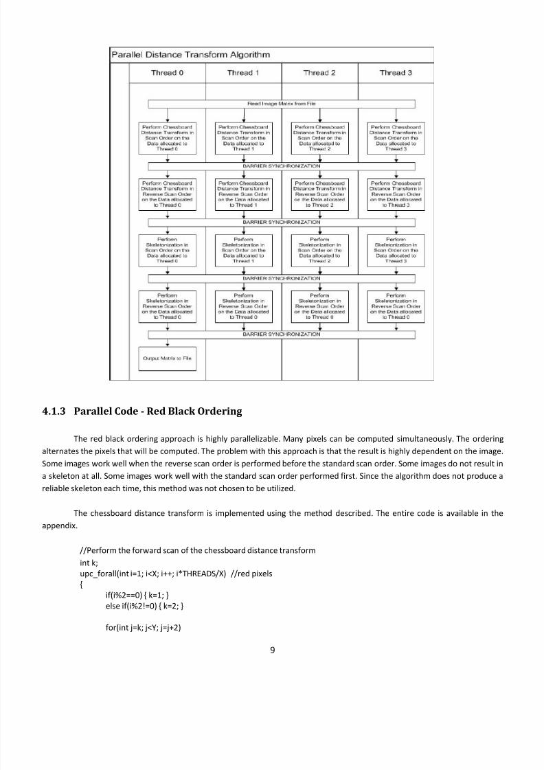
4.1.3 Parallel Code - Red Black Ordering

The red black ordering approach is highly parallelizable. Many pixels can be computed simultaneously. The ordering

alternates the pixels that will be computed. The problem with this approach is that the result is highly dependent on the image.

Some images work well when the reverse scan order is performed before the standard scan order. Some images do not result in

a skeleton at all. Some images work well with the standard scan order performed first. Since the algorithm does not produce a

reliable skeleton each time, this method was not chosen to be utilized.

The chessboard distance transform is implemented using the method described. The entire code is available in the

appendix.

//Perform the forward scan of the chessboard distance transform

int k;

upc_forall(int i=1; i<X; i++; i*THREADS/X) //red pixels

{

if(i%2==0) { k=1; }

else if(i%2!=0) { k=2; }

for(int j=k; j<Y; j=j+2)



10

{

if(A[i][j]==1)

{

int min=A[i‐1][j];

if(A[i‐1][j] < min) min = A[i‐1][j];

if(A[i][j‐1] < min) min = A[i][j‐1];

A[i][j] = min + 1;

}

}

}

upc_barrier;

upc_forall(int i=1; i<X; i++; i*THREADS/X) //black pixels

{

if(i%2==0) { k=2; }

else if(i%2!=0) { k=1; }

for(int j=k; j<Y; j=j+2)

{

if(A[i][j]==1)

{ int min=A[i‐1][j];

if(A[i‐1][j] < min) min = A[i‐1][j];

if(A[i][j‐1] < min) min = A[i][j‐1];

A[i][j] = min + 1;

}

}

}

//Perform reverse scan of the chessboard distance transform

upc_forall(int i=X‐1; i>0; i‐‐; i*THREADS/X) //red pixels

{

if(i%2==0) { k=1; }

else if(i%2!=0)

{ k=2;

}

for(int j=Y‐k; j>0; j=j‐2)

{

if(A[i][j]>1)

{

int min = A[i][j+1];

if(A[i+1][j] < min) min = A[i+1][j];

if(min+1 < A[i][j]) A[i][j] = min + 1;

}

}

}

upc_barrier;

upc_forall(int i=X‐1; i>0; i‐‐; i*THREADS/X) //black pixels

{

if(i%2==0) { k=2; }

else if(i%2!=0) { k=1; }

for(int j=Y‐k; j>0; j=j‐2)

{



11

if(A[i][j]>1)

{

int min = A[i][j+1];

if(A[i+1][j] < min) min = A[i+1][j];

if(min+1 < A[i][j]) A[i][j] = min + 1;

}

}

}

The skeletonization process stays the same for the red‐black ordering algorithm. Changes are only made to the

chessboard distance transform part of the program.

4.2 Parallelization of Thinning Algorithm

Thinning or erosion of the image is a method that iteratively peels off the boundary layer by layer from outside to

inside. The removal does not affect the topology of the image. This is a repetitive and time‐consuming process of testing and

deletion of each pixel. It is good for connectivity preservation. The problem with this approach is that the set of rules defining

the removal of a pixel is highly dependent on the type of image and different set of rules will be applied for different types of

images. Thinning is best when performed on alphabets and numbers.

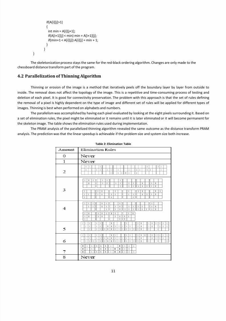
The parallelism

was

accomplished

by

having

each

pixel

evaluated

by

looking

at

the

eight

pixels

surrounding

it.

Based

on

a set of elimination rules, the pixel might be eliminated or it remains until it is later eliminated or it will become permanent for

the skeleton image. The table shows the elimination rules used during implementation.

The PRAM analysis of the parallelized thinning algorithm revealed the same outcome as the distance transform PRAM

analysis. The prediction was that the linear speedup is achievable if the problem size and system size both increase.

Table 2: Elimination Table



12

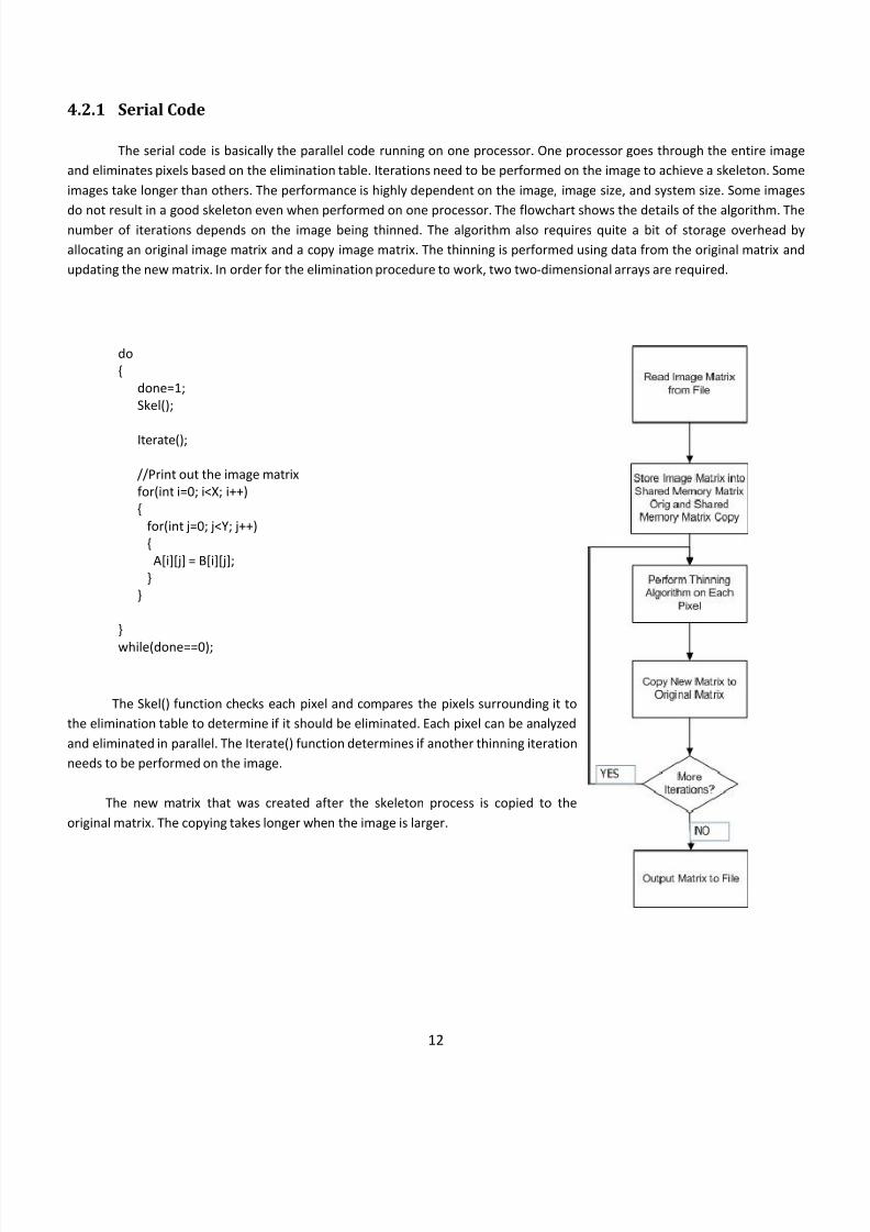
4.2.1 Serial Code

The serial code is basically the parallel code running on one processor. One processor goes through the entire image

and eliminates pixels based on the elimination table. Iterations need to be performed on the image to achieve a skeleton. Some

images take longer than others. The performance is highly dependent on the image, image size, and system size. Some images

do

not

result

in

a

good

skeleton

even

when

performed

on

one

processor.

The

flowchart

shows

the

details

of

the

algorithm.

The

number of iterations depends on the image being thinned. The algorithm also requires quite a bit of storage overhead by

allocating an original image matrix and a copy image matrix. The thinning is performed using data from the original matrix and

updating the new matrix. In order for the elimination procedure to work, two two‐dimensional arrays are required.

do

{

done=1;

Skel();

Iterate();

//Print out the image matrix

for(int i=0; i<X; i++)

{

for(int j=0; j<Y; j++)

{

A[i][j] = B[i][j];

}

}

}

while(done==0);

The Skel() function checks each pixel and compares the pixels surrounding it to

the elimination table to determine if it should be eliminated. Each pixel can be analyzed

and eliminated in parallel. The Iterate() function determines if another thinning iteration

needs to be performed on the image.

The new matrix that was created after the skeleton process is copied to the

original matrix. The copying takes longer when the image is larger.



13

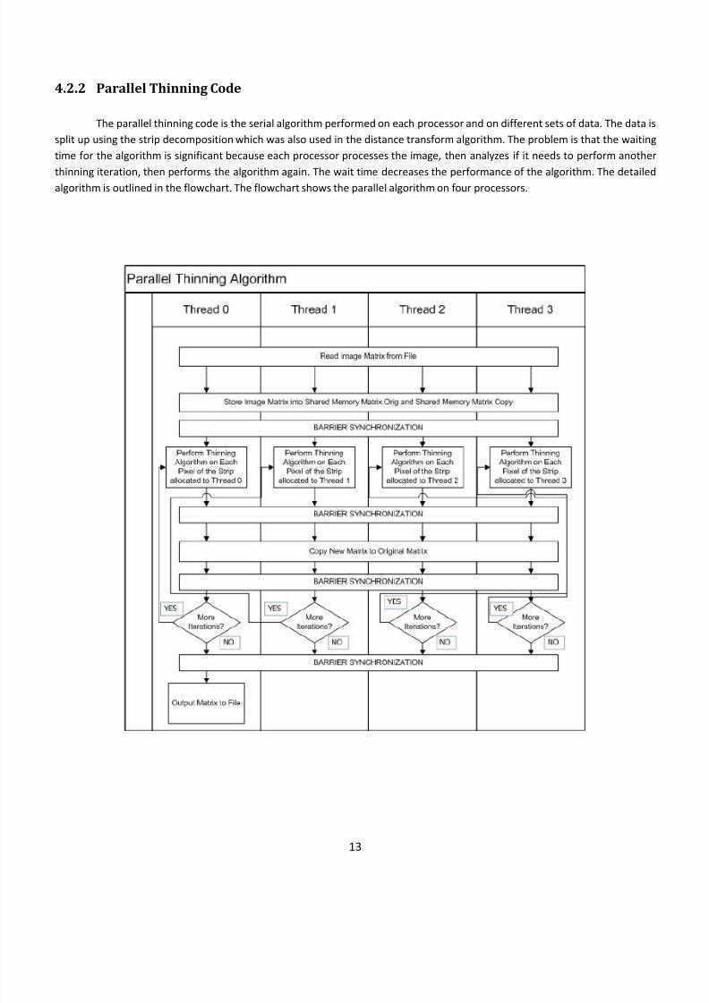
4.2.2 Parallel Thinning Code

The parallel thinning code is the serial algorithm performed on each processor and on different sets of data. The data is

split up using the strip decomposition which was also used in the distance transform algorithm. The problem is that the waiting

time for the algorithm is significant because each processor processes the image, then analyzes if it needs to perform another

thinning

iteration,

then

performs

the

algorithm

again.

The

wait

time

decreases

the

performance

of

the

algorithm.

The

detailed

algorithm is outlined in the flowchart. The flowchart shows the parallel algorithm on four processors.



14

5. Comparison of Distance Transform and Thinning Algorithms

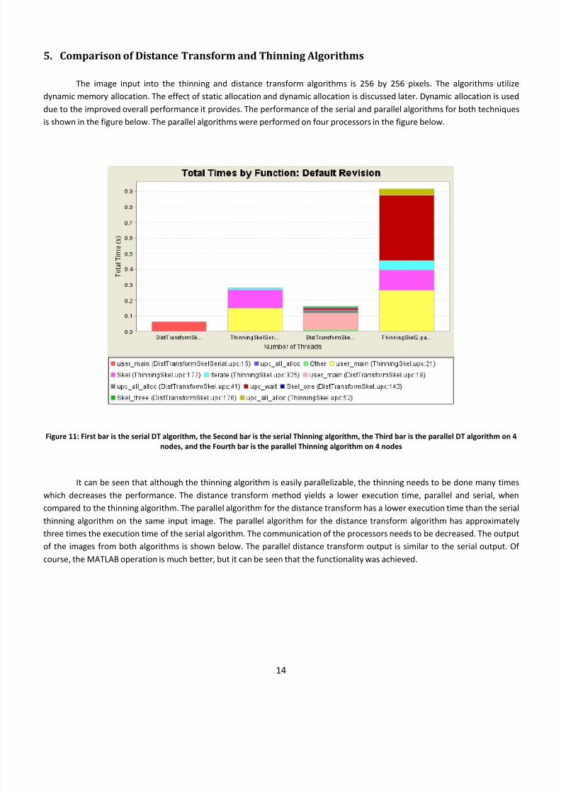
The image input into the thinning and distance transform algorithms is 256 by 256 pixels. The algorithms utilize

dynamic memory allocation. The effect of static allocation and dynamic allocation is discussed later. Dynamic allocation is used

due to the improved overall performance it provides. The performance of the serial and parallel algorithms for both techniques

is shown in the figure below. The parallel algorithms were performed on four processors in the figure below.

Figure 11: First bar is the serial DT algorithm, the Second bar is the serial Thinning algorithm, the Third bar is the parallel DT algorithm on 4

nodes, and the Fourth bar is the parallel Thinning algorithm on 4 nodes

It can be seen that although the thinning algorithm is easily parallelizable, the thinning needs to be done many times

which decreases the performance. The distance transform method yields a lower execution time, parallel and serial, when

compared to the thinning algorithm. The parallel algorithm for the distance transform has a lower execution time than the serial

thinning algorithm on the same input image. The parallel algorithm for the distance transform algorithm has approximately

three times the execution time of the serial algorithm. The communication of the processors needs to be decreased. The output

of the images from both algorithms is shown below. The parallel distance transform output is similar to the serial output. Of

course, the

MATLAB

operation

is

much

better,

but

it

can

be

seen

that

the

functionality

was

achieved.



15

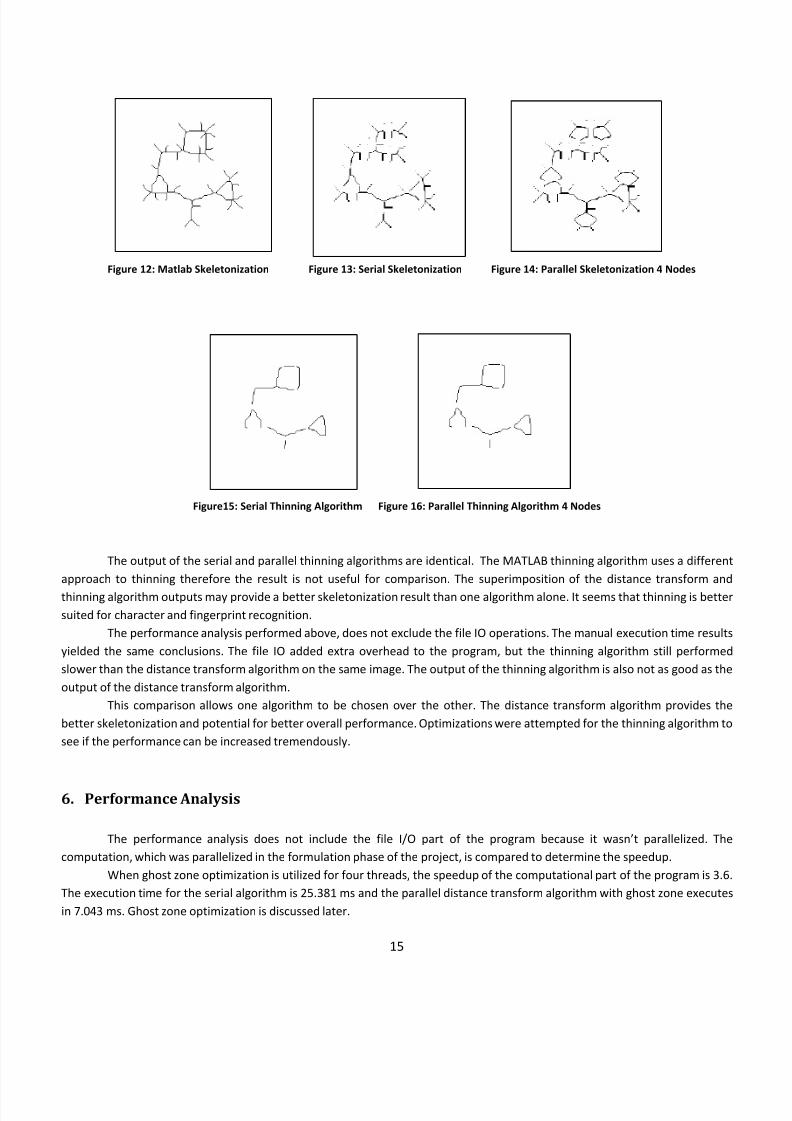
Figure 12: Matlab Skeletonization Figure 13: Serial Skeletonization Figure 14: Parallel Skeletonization 4 Nodes

Figure15: Serial Thinning Algorithm Figure 16: Parallel Thinning Algorithm 4 Nodes

The output of the serial and parallel thinning algorithms are identical. The MATLAB thinning algorithm uses a different

approach to thinning therefore the result is not useful for comparison. The superimposition of the distance transform and

thinning algorithm outputs may provide a better skeletonization result than one algorithm alone. It seems that thinning is better

suited for character and fingerprint recognition.

The performance analysis performed above, does not exclude the file IO operations. The manual execution time results

yielded the same conclusions. The file IO added extra overhead to the program, but the thinning algorithm still performed

slower than the distance transform algorithm on the same image. The output of the thinning algorithm is also not as good as the

output of the distance transform algorithm.

This comparison allows one algorithm to be chosen over the other. The distance transform algorithm provides the

better skeletonization and potential for better overall performance. Optimizations were attempted for the thinning algorithm to

see if the performance can be increased tremendously.

6. Performance Analysis The performance analysis does not include the file I/O part of the program because it wasn’t parallelized. The

computation, which was parallelized in the formulation phase of the project, is compared to determine the speedup.

When ghost zone optimization is utilized for four threads, the speedup of the computational part of the program is 3.6.

The execution time for the serial algorithm is 25.381 ms and the parallel distance transform algorithm with ghost zone executes

in 7.043 ms. Ghost zone optimization is discussed later.



16

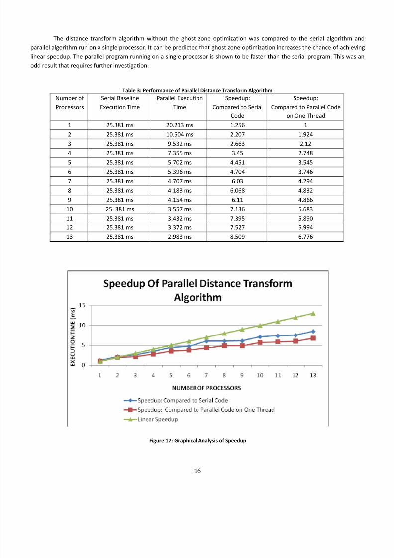
The distance transform algorithm without the ghost zone optimization was compared to the serial algorithm and

parallel algorithm run on a single processor. It can be predicted that ghost zone optimization increases the chance of achieving

linear speedup. The parallel program running on a single processor is shown to be faster than the serial program. This was an

odd result that requires further investigation.

Table 3: Performance of Parallel Distance Transform Algorithm

Number of

Processors Serial

Baseline

Execution Time

Parallel Execution

Time

Speedup:

Compared to Serial

Code

Speedup:

Compared to Parallel Code

on One Thread

1 25.381 ms 20.213 ms 1.256 1

2 25.381 ms 10.504 ms 2.207 1.924

3 25.381 ms 9.532 ms 2.663 2.12

4 25.381 ms 7.355 ms 3.45 2.748

5 25.381 ms 5.702 ms 4.451 3.545

6 25.381 ms 5.396 ms 4.704 3.746

7 25.381 ms 4.707 ms 6.03 4.294

8 25.381 ms 4.183 ms 6.068 4.832

9 25.381 ms 4.154 ms 6.11 4.866

10 25. 381 ms 3.557 ms 7.136 5.683

11 25.381 ms 3.432 ms 7.395 5.890

12 25.381 ms 3.372 ms 7.527 5.994

13 25.381 ms 2.983 ms 8.509 6.776

Figure 17: Graphical Analysis of Speedup



17

It seems that the communication increases as the number of processors increase. This communication is limiting the

approach to linear speedup. Another problem is that the algorithm used doesn’t consider data dependencies. Therefore as the

number of processors becomes larger than 15 processors, the image is significantly different from the serial baseline image. The

user can make a compromise and achieve four to five times speedup on five to six processors and still achieve the image

required.

7. Optimization of Algorithms

Both algorithms were optimized to analyze the performance increase. Thinning algorithm optimizations were

performed, in case the performance greatly increases after performing the optimization. Some optimizations relate to both

algorithms and were performed to see the impact it would have on overall performance. The common optimizations to both

algorithms are described below.

Experiment 1: Investigate the best configuration with Dynamic Memory Allocation for Both Algorithms

Dynamic memory allocation was investigated to optimize the memory on the threads. The best optimization for the

parallel thinning

algorithm

that

could

be

achieved

was

0.91325

seconds.

The

serial

thinning

algorithm

had

an

overall

execution

time of 280.5 milliseconds.

The other memory distributions didn’t reduce the communication overhead. The same was seen with the distance

transform algorithm. The best configuration resulted in 160 ms of overall execution time.

A=(shared int **)upc_all_alloc(THREADS, X*sizeof(int *));

for(i = 0; i < X; i++)

{

A[i] = (shared int *)upc_all_alloc(THREADS, Y*sizeof(int));

for(j = 0; j < Y; j++)

{

int temp;

fscanf(fpt, "%d", &temp);

A[i][j] = temp;

}

}

Experiment 2: Attempt to Parallelize the File I/O Operations

It was attempted to make each thread only read in the data necessary for most of its computation. This will cause the

execution time to decrease. The parallel I/O operations were not working as needed. The file reading was not being properly

done. The data from the file does not match with the data found in the vector. Since there are problems, focus has been turned

to reducing the communication and hiding that communication behind computation.

Much of the other processing besides the computation is the file input and output. All the processors need to be aware

of the file and open it. Parallelizing this will significantly improve the performance of the parallel program. When the

functionality of this improves, then it can be used to decrease the file I/O aspect of the program.



18

7.1 Thinning Algorithm

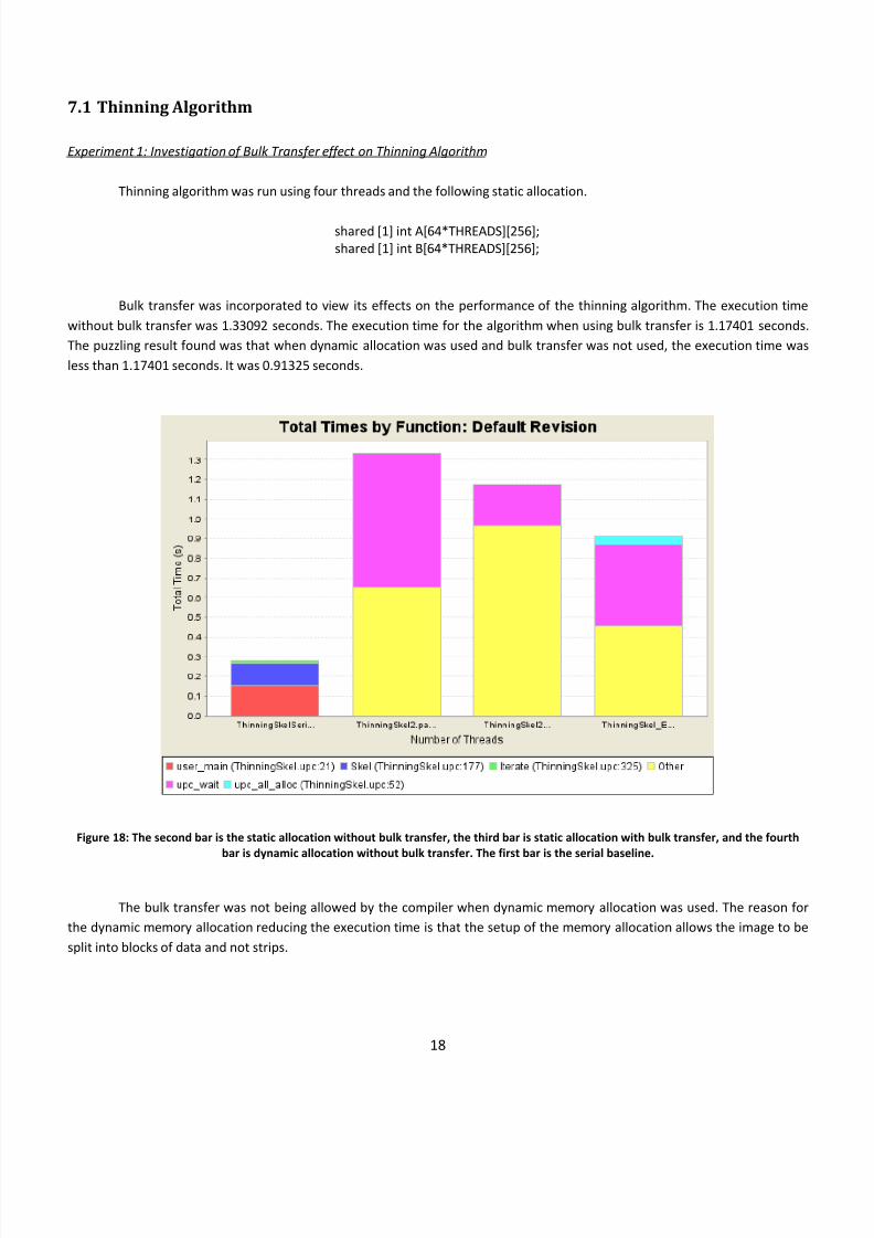
Experiment 1: Investigation of Bulk Transfer effect on Thinning Algorithm Thinning algorithm was run using four threads and the following static allocation.

shared [1] int A[64*THREADS][256];

shared [1] int B[64*THREADS][256];

Bulk transfer was incorporated to view its effects on the performance of the thinning algorithm. The execution time

without bulk transfer was 1.33092 seconds. The execution time for the algorithm when using bulk transfer is 1.17401 seconds.

The puzzling result found was that when dynamic allocation was used and bulk transfer was not used, the execution time was

less than 1.17401 seconds. It was 0.91325 seconds.

Figure 18: The second bar is the static allocation without bulk transfer, the third bar is static allocation with bulk transfer, and the fourth

bar is dynamic allocation without bulk transfer. The first bar is the serial baseline.

The bulk transfer was not being allowed by the compiler when dynamic memory allocation was used. The reason for

the dynamic memory allocation reducing the execution time is that the setup of the memory allocation allows the image to be

split into blocks of data and not strips.



19

7.2 Distance Transform Algorithm

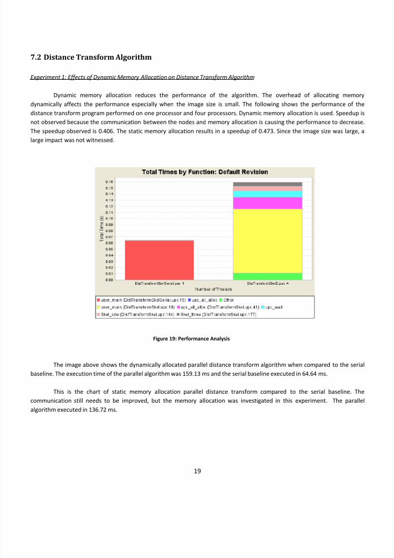
Experiment 1: Effects of Dynamic Memory Allocation on Distance Transform Algorithm

Dynamic

memory

allocation

reduces

the

performance

of

the

algorithm.

The

overhead

of

allocating

memory

dynamically affects the performance especially when the image size is small. The following shows the performance of the

distance transform program performed on one processor and four processors. Dynamic memory allocation is used. Speedup is

not observed because the communication between the nodes and memory allocation is causing the performance to decrease.

The speedup observed is 0.406. The static memory allocation results in a speedup of 0.473. Since the image size was large, a

large impact was not witnessed.

The image above shows the dynamically allocated parallel distance transform algorithm when compared to the serial

baseline. The execution time of the parallel algorithm was 159.13 ms and the serial baseline executed in 64.64 ms.

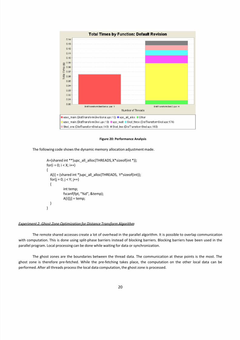
This

is

the

chart

of

static

memory

allocation

parallel

distance

transform

compared

to

the

serial

baseline.

The

communication still needs to be improved, but the memory allocation was investigated in this experiment. The parallel

algorithm executed in 136.72 ms.

Figure 19: Performance Analysis



20

The following code shows the dynamic memory allocation adjustment made.

A=(shared int **)upc_all_alloc(THREADS, X*sizeof(int *));

for(i = 0; i < X; i++)

{

A[i] = (shared int *)upc_all_alloc(THREADS, Y*sizeof(int));

for(j = 0;

j < Y;

j++)

{

int temp;

fscanf(fpt, "%d", &temp);

A[i][j] = temp;

}

}

Experiment 2: Ghost Zone Optimization for Distance Transform Algorithm

The remote shared accesses create a lot of overhead in the parallel algorithm. It is possible to overlap communication

with computation.

This

is

done

using

split

‐phase

barriers

instead

of

blocking

barriers.

Blocking

barriers

have

been

used

in

the

parallel program. Local processing can be done while waiting for data or synchronization.

The ghost zones are the boundaries between the thread data. The communication at these points is the most. The

ghost zone is therefore pre‐fetched. While the pre‐fetching takes place, the computation on the other local data can be

performed. After all threads process the local data computation, the ghost zone is processed.




21

The execution time of the parallel distance transform algorithm drops to 107.41 ms. The ghost zone execution is good

for performance improvement, but the improvement will be more visible when there are more processors and larger images.

The

speedup

is

0.602.

Figure 21: Ghost Zone




22

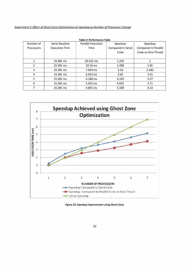
Experiment 3: Effect of Ghost Zone Optimization on Speedup as Number of Processors Change

Table 4: Performance Table

Number of

Processors

Serial Baseline

Execution Time

Parallel Execution

Time

Speedup:

Compared to

Serial

Code

Speedup:

Compared to

Parallel

Code on One Thread

1 25.381 ms 20.232 ms 1.254 1

2 25.381 ms 10.16 ms 2.498 1.99

3 25.381 ms 7.834 ms 3.24 2.582

4 25.381 ms 6.953 ms 3.65 2.91

5 25.381 ms 6.186 ms 4.103 3.27

6 25.381 ms 5.452 ms 4.655 3.71

7 25.381 ms 4.891 ms 5.189 4.14

Figure 23: Speedup Improvement using Ghost Zone



23

8. Conclusion

The analysis of both pixel‐based algorithms revealed that parallelization will cause performance

improvement but it will not be linear. After implementation, optimization and analysis, it was found that the best

algorithm

is

the

distance

transform

algorithm

when

executed

on

five

to

six

processors.

The

performance

and

accuracy are decent at this system size. The optimizations can be further investigated to achieve linear speedup.

Many different methods, such as parallel file I/O, can speed up the algorithm tremendously. Future work should

focus on obtaining linear speedup on a small system size. Based on preliminary results, it seems possible to achieve

the goal.

9. References

[1] “An effective skeletonization method based on adaptive selection of contour points”

Morrison, P.; Ju Jia Zou; Information Technology and Applications, 2005. ICITA 2005. Third International Conference

on Volume 1, 4‐7 July 2005 Page(s):644 ‐ 649 vol.1

[2] “Parallel digital signal processing: an emerging market.” 24 Feb 2008.

<http://focus.ti.com/lit/an/spra104/spra104.pdf>

[3] “Efficient 3D binary image skeletonization” Tran, S.; Shih, L.; Computational Systems

Bioinformatics Conference, 2005. Workshops and Poster Abstracts. IEEE 8‐11 Aug. 2005 Page(s):364 ‐ 372

[4] "Binary image." Wikipedia, The Free Encyclopedia. 17 Jan 2008, 21:52 UTC. Wikimedia

Foundation, Inc. 24 Feb 2008 <http://en.wikipedia.org/w/index.php?title=Binary_image&oldid=185070806>.

[5] “Skeletonization.” 24 Feb 2008. <http://www.inf.u‐szeged.hu/~palagyi/skel/skel.html>

[6] "Distance transform." Wikipedia, The Free Encyclopedia. 20 Feb 2008, 07:22 UTC.

Wikimedia Foundation, Inc. 24 Feb 2008

<http://en.wikipedia.org/w/index.php?title=Distance_transform&oldid=192754303>.

[7] “Marvel Machine.” High Performance Computing and Simulation Lab. 24 Feb 2008

< http://www.hcs.ufl.edu/lab/marvel.php>

[8] “Skeletonization by blocks for large 3D datasets: application to brain microcirculation”

Fouard, C.; Cassot, E.; Malandain, G.; Mazel, C.; Prohaska, S.; Asselot, D.; Westerhoff, M.; Marc‐Vergnes, J.P.;

Biomedical Imaging: Macro to Nano, 2004. IEEE International Symposium on 15‐18 April 2004 Page(s):89 ‐ 92 Vol. 1

Documents

on of Two-Dimensional Skeletonization Algorithms - IEEE