Embed Size (px)
Citation preview
On Rank Problems for Subspaces of Matricesover Finite Fields
by
John Sheekey
A dissertation presented to
University College Dublin in partial
fulfillment of the requirements for the degree of
Doctor of Philosophy
in the College of Engineering, Mathematical
and Physical Sciences
August 2011
School of Mathematical Sciences
Head of School: Dr. Mıcheal O Searcoid
Supervisor of Research: Professor Roderick Gow
Contents
Table of Contents . . . . . . . . . . . . . . . . . . . . . . . . . . . . . . . . iiAcknowledgements . . . . . . . . . . . . . . . . . . . . . . . . . . . . . . . iiiAbstract . . . . . . . . . . . . . . . . . . . . . . . . . . . . . . . . . . . . . iv
1 Introduction to constant rank subspaces 11.1 Constant rank subspaces . . . . . . . . . . . . . . . . . . . . . . . . . 11.2 Symmetric bilinear forms and quadratic forms . . . . . . . . . . . . . 51.3 Subspaces of matrices as codes . . . . . . . . . . . . . . . . . . . . . 13
2 Semifields and constant rank subspaces 162.1 Semifields . . . . . . . . . . . . . . . . . . . . . . . . . . . . . . . . . 162.2 Semifields as subspaces of matrices . . . . . . . . . . . . . . . . . . . 21
3 Constant rank subspaces of symmetric and hermitian matrices 263.1 Counting theorem for subspaces of function spaces . . . . . . . . . . 263.2 Bounds for constant rank subspaces . . . . . . . . . . . . . . . . . . 293.3 Constant rank 3 spaces of symmetric matrices over arbitrary fields . 39
4 Primitive elements in finite semifields 454.1 Primitive elements . . . . . . . . . . . . . . . . . . . . . . . . . . . . 454.2 Primitive element theorems . . . . . . . . . . . . . . . . . . . . . . . 51
5 Semifields from skew-polynomial rings 545.1 Skew-polynomial rings . . . . . . . . . . . . . . . . . . . . . . . . . . 545.2 Connections with known constructions . . . . . . . . . . . . . . . . . 62
6 Isotopy classes of semifields from skew-polynomial rings 746.1 Isotopy relations . . . . . . . . . . . . . . . . . . . . . . . . . . . . . 746.2 Counting isotopy classes for finite semifields . . . . . . . . . . . . . . 76
Bibliography 88
ii
Acknowledgements
This thesis would not have been possible without the help and support of all my
family, friends, colleagues and teachers.
Thank you to my parents, Peter and Theresa, for their unwavering and unconditional
support. To everyone at UCD, I could not have wished for a better place to spend
four years of my life.
To all my teachers, mentors and co-authors, for their willingness to share their
wisdom, and for inspiring me to pursue a career in mathematics. In particular to my
supervisor, Rod Gow, for his unfailing enthusiasm and patience, and his generosity
with his time and knowledge.
iii
Abstract
In this thesis we are concerned with themes suggested by rank properties of subspaces
of matrices. Historically, most work on these topics has been devoted to matrices over
such fields as the real or complex numbers, where geometric or analytic methods may
be applied. Such techniques are not obviously applicable to finite fields, and there
were very few general theorems relating to rank problems over finite fields.
In this thesis we are concerned mainly with constant rank subspaces of matrices over
finite fields, with particular focus on two subcases: (1) constant rank subspaces of
symmetric or hermitian matrices; and (2) constant full rank subspaces of matrices,
which correspond to nonassociative algebraic structures known as semifields.
In Chapter 1 we will introduce constant rank subspaces of matrices, and review the
known results on the maximum dimension of such a subspace. In Chapter 2 we will
recall the definition of a semifield, and illustrate how these algebraic structures are
related to constant rank subspaces of matrices.
In Chapter 3 we will prove a general theorem on subspaces of function spaces, and
apply the results to obtain new upper bounds on subspaces of matrices, which are
sharp in some cases.
In Chapter 4 we will study primitive elements in finite semifields, and prove their
existence for a certain family of semifields. In Chapters 5 and 6 we will introduce a
construction for semifields using skew-polynomial rings. We will show how they are
related to other known constructions, use this representation to obtain new results,
and provide elegant new proofs for some known results.
iv
Chapter 1
Introduction to constant rank
subspaces
In this chapter we will define constant rank subspaces, establish some notation,
survey the known results and applications, and introduce some concepts and results
which will be needed in subsequent chapters.
1.1 Constant rank subspaces
1.1.1 Definitions and Notations
Let F denote an arbitrary field, Mm×n(F) denote the space of m× n matrices over
F, and Mn(F) := Mn×n(F), where m and n are positive integers. We will assume
unless otherwise stated that m ≤ n. For any non-zero subspace U of Mm×n(F) let
U× denote the subset of non-zero elements in U .
Let V denote a vector space n-dimensional over F. Let K denote an extension field
of F of degree 2 (assuming such an extension exists), and let W denote a vector
space n-dimensional over K.
We denote the space of n×n symmetric matrices over F by Sn(F). If F has a degree
1
Chapter 1: Introduction to constant rank subspaces
2 extension K admitting an F-automorphism of order 2, we denote the space of n×nhermitian matrices over K by Hn(F). Note that Hn(F) is not a vector space over K,
but is a vector space over F of dimension n2. Note that the notation is potentially
ambiguous, since such an extension field K need not be unique. However, in this
work we will only be considering hermitian matrices over finite fields, which of course
possess a unique degree 2 extension.
Let p be a prime, q a power of p. Let Fq denote the finite field of q elements.
Definition 1.1. Let U be a non-zero subspace of Mm×n(F). We say that U is a
constant rank r subspace if every element of U× has rank r.
Much research has been done to investigate the maximum possible dimension of a
constant rank r subspace. The results and techniques differ greatly according to
properties of the underlying field.
We will focus on constant rank subspaces of Mm×n(F), Sn(F) and Hn(F), with
particular attention to finite fields and constant rank n subspaces.
1.1.2 Existing bounds for the maximum dimension of constant rank
subspaces
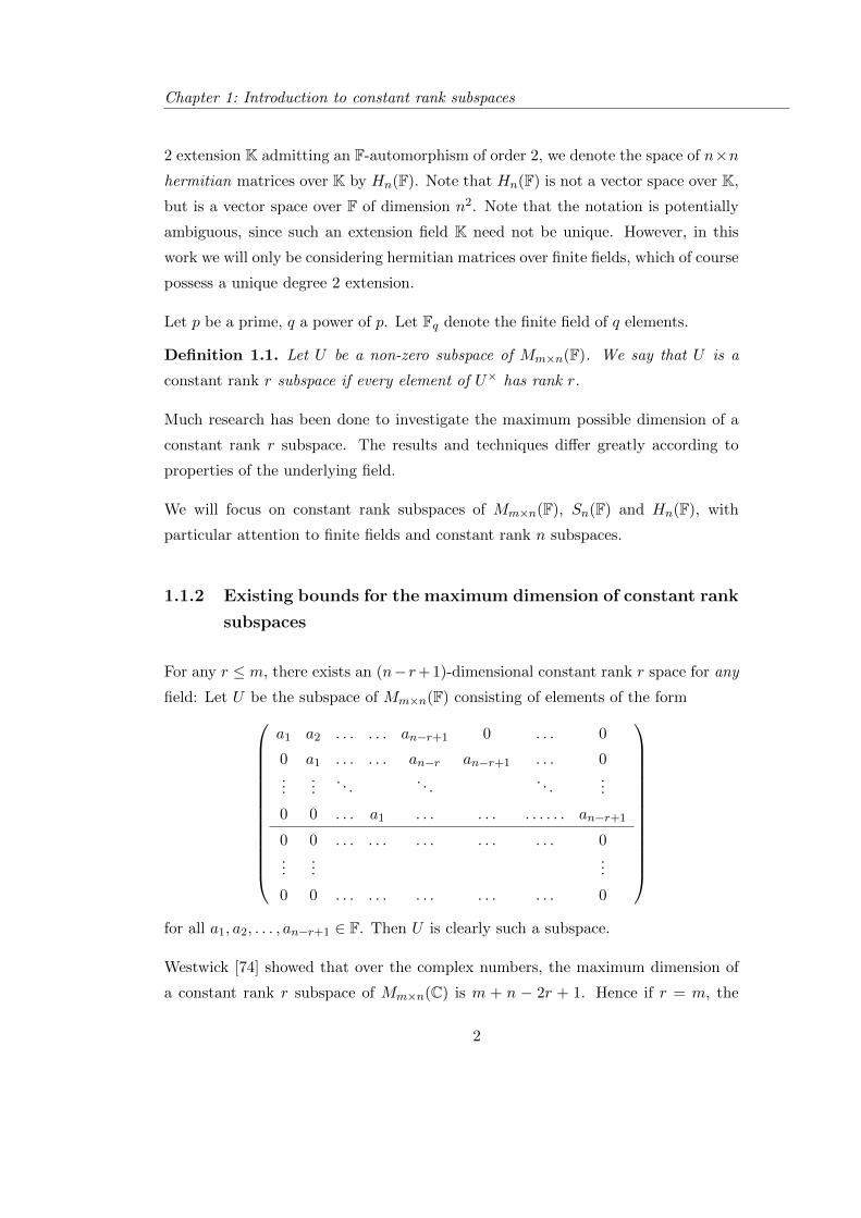
For any r ≤ m, there exists an (n−r+1)-dimensional constant rank r space for any
field: Let U be the subspace of Mm×n(F) consisting of elements of the form
a1 a2 . . . . . . an−r+1 0 . . . 0
0 a1 . . . . . . an−r an−r+1 . . . 0...
.... . .
. . .. . .
...
0 0 . . . a1 . . . . . . . . . . . . an−r+1
0 0 . . . . . . . . . . . . . . . 0...
......
0 0 . . . . . . . . . . . . . . . 0
for all a1, a2, . . . , an−r+1 ∈ F. Then U is clearly such a subspace.
Westwick [74] showed that over the complex numbers, the maximum dimension of
a constant rank r subspace of Mm×n(C) is m + n − 2r + 1. Hence if r = m, the
2
Chapter 1: Introduction to constant rank subspaces
above construction is optimal. Ilic and Landsberg [34] showed that the maximum
dimension of a constant rank r subspace of Sn(C) is n − r + 1 if r is even, using
techniques of complex algebraic geometry. The maximum dimension of a constant
rank r subspace of Sn(C) or Sn(R) is 1 if r is odd. We will discuss the case where
r is odd further in Section 3.3.2. Much study has been dedicated to the problem of
constant rank subspaces over R and C, for example in [5], [12], [48], [57], [74], [75].
Large constant rank spaces can be constructed using division algebras defined over
F (see Corollary 2.8).
Lemma 1.2. Suppose there exist an n-dimensional constant rank n subspace U of
Mn(F). Then for any 1 ≤ r ≤ m ≤ n there exists an n-dimensional constant rank r
subspace U ′ of Mm×n(F).
Proof. Let A be an arbitrary rank r element of Mm×n(F). Let
U ′ = AX : X ∈ U.
It is clear that every non-zero element of U ′ has rank r. It remains to show that
dim(U ′) = n. Suppose AX = AY for some X,Y ∈ U , X 6= Y . Then A(X −Y ) = 0.
But 0 6= X − Y ∈ U , and so X − Y is invertible. But then we must have A = 0,
a contradiction. Hence the map from U to U ′ defined by X 7→ AX is injective and
surjective, implying dim(U ′) = dim(U) = n and hence proving the result.
A presemifield is a division algebra where multiplication is not assumed to be asso-
ciative, and a multiplicative identity is not assumed to exist. These structures will
be defined and discussed in Chapter 2, and the following theorem is well known and
will be proved.
Theorem 1.3. There exist an n-dimensional constant rank n subspace of Mn(F) if
and only if there exists a presemifield n-dimensional over F.
Note that a field is certainly a presemifield. As every finite field admits an extension
field of degree n for all n, we have the following theorem:
Theorem 1.4. For every 1 ≤ r ≤ m ≤ n there exists an n-dimensional constant
rank r subspace of Mm×n(Fq) for all q.
3
Chapter 1: Introduction to constant rank subspaces
Beasley and Laffey showed in [5] that this dimension bound is optimal when the
conditions |F| ≥ r + 1 and n ≥ 2r − 1 are imposed. We will see a similar restriction
on field size later in Section 3.3. This restriction is imposed to ensure the existence
of a non-root of a polynomial of degree r.
Theorem 1.5. Suppose |F| ≥ r + 1 and n ≥ 2r − 1. Suppose U is a constant rank
r subspace of Mm×n(F). Then dim(U) ≤ n.
In [26] the following upper bound was proved for finite fields:
Theorem 1.6. Let U be a constant rank r subspace of Mm×n(Fq). Then dim(U) ≤m+ n− r.
This bound was proved via character theory, using character values calculated by
Delsarte in [16]. In Section 3.2.1 we will provide an new proof of this theorem.
The above bounds do not rule out the possibility of constant rank r subspaces of
n × n matrices of dimension larger than n if r is large, or the field size is small.
Indeed there exist subspaces which meet the bound of Theorem 1.6 over the field of
two elements, as shown in [6], [7], [26].
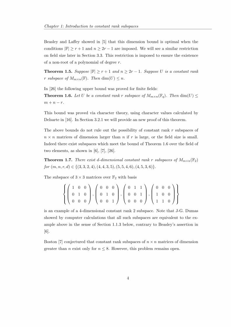
Theorem 1.7. There exist d-dimensional constant rank r subspaces of Mm×n(F2)
for (m,n, r, d) ∈ (3, 3, 2, 4), (4, 4, 3, 5), (5, 5, 4, 6), (4, 5, 3, 6).
The subspace of 3× 3 matrices over F2 with basis
1 0 0
0 1 0
0 0 0
,
0 0 0
0 1 0
0 0 1
,
0 1 1
0 0 1
0 0 0
,
0 0 0
1 0 0
1 1 0
is an example of a 4-dimensional constant rank 2 subspace. Note that J-G. Dumas
showed by computer calculations that all such subspaces are equivalent to the ex-
ample above in the sense of Section 1.1.3 below, contrary to Beasley’s assertion in
[6].
Boston [7] conjectured that constant rank subspaces of n× n matrices of dimension
greater than n exist only for n ≤ 8. However, this problem remains open.
4
Chapter 1: Introduction to constant rank subspaces
1.1.3 Equivalence
We consider some linear maps on Mm×n(F) which preserve rank. Let X and Y be
invertible elements of Mm(F) and Mn(F) respectively. Then the maps
A 7→ XA
A 7→ AY
clearly preserve rank.
Let σ be an automorphism of F. For A ∈ Mm×n(F), define Aσ to be the matrix
obtained by applying σ to every entry of A. Then the map A 7→ Aσ is also a linear
map which preserves rank.
Clearly these above maps generate a group E of linear maps which preserve rank,
consisting of elements of the form φX,Y,σ : A 7→ XAσY .
We can extend these maps to subspaces of matrices. Let φ ∈ E, and U a subspace
of Mm×n(F). Then define
U 7→ Uφ := Aφ : A ∈ U.
Clearly U is a constant rank r subspace if and only if Uφ is a constant rank r
subspace.
We say that two subspaces U and U ′ are equivalent if there exists an element φ ∈ Esuch that U ′ = Uφ.
Note that if m = n, then the map sending each matrix to its transpose, A 7→ AT ,
is another linear map which preserves rank. However, we will exclude these maps
from the definition of equivalence of subspaces.
1.2 Symmetric bilinear forms and quadratic forms
In this section we will recall the connections between symmetric matrices, bilinear
forms, and quadratic forms, which we will exploit later in this work.
5
Chapter 1: Introduction to constant rank subspaces
1.2.1 Bilinear forms
Definition 1.8. Let V be a vector space n-dimensional over a field F. A bilinear
form is a map B : V × V → F such that
B(u+ v, w) = B(u,w) + B(v, w)
B(u, v + w) = B(u, v) + B(u,w)
B(λu, v) = B(u, λv) = λB(u, v)
for all u, v, w ∈ V , and all λ ∈ F.
Denote the set of all bilinear form on V ×V by Bn(F). It is well known that bilinear
forms are related to matrices in the following way: let e1, e2, . . . , en be an F-
basis for V . Let u and v be elements of V , and suppose u =∑
i uiei, v =∑
i viei
for ui, vi ∈ F. Then by the above defining properties of bilinear forms, we have
that
B(u, v) =
n∑i,j=1
uivjB(ei, ej).
Hence the action of B is completely determined by its action on all pairs of basis
elements. Define bij := B(ei, ej) for each i, j. Then the above can be written
as
B(u, v) =
n∑i,j=1
uivjbij . (1.1)
Consider now the matrix B := (bij)i,j ∈Mn(F). Identify each element u =∑
i uiei ∈V with the column vector
u =
u1
u2
...
un
.
Then it is clear from the definition of matrix multiplication and equation 1.1 that
B(u, v) = uTBv. (1.2)
Note that the entries of the matrix B depends on the choice of basis. Hence we refer
to B as the matrix representing B with respect to the basis e1, e2, . . . , en. Suppose
e′1, e′2, . . . , e′n is another F-basis for V , and let B′ be the matrix representing B
6
Chapter 1: Introduction to constant rank subspaces
with respect to this basis. Then if we let X denote the change of basis matrix, it is
clear that
B′ = XTBX.
Conversely, clearly every n× n matrix over F defines a bilinear form in the manner
of equation 1.2. Hence the Bn(F) can be identified with Mn(F) through the choice
of a basis for V . Similarly, if V ′ is a vector space m-dimensional vector space over
F, we can define Bm×n(F) to be the set of bilinear forms on V ′ × V , and identify
Bm×n(F) 'Mm×n(F), where ‘'’ denotes F-isomorphism of vector spaces.
1.2.2 Symmetric matrices and quadratic forms
A bilinear form B is said to be symmetric if B(u, v) = B(v, u) for all u, v ∈ V . Denote
the set of symmetric bilinear forms by Sn(F). It is clear from the definitions that
if B represents B with respect to some basis, then B is a symmetric bilinear form
if and only if B = BT , i.e. B is a symmetric matrix. Conversely, every symmetric
matrix defines a symmetric bilinear form. Hence we can see that
Sn(F) ' Sn(F).
Definition 1.9. A quadratic form is a function Q : V → F such that
Q(λu+ µv) = λ2Q(u) + µ2Q(v) + λµBQ(u, v), (1.3)
where BQ is a bilinear form on V × V .
We call BQ the associated bilinear form (or polarization) of Q. The set of quadratic
forms on V forms an F-vector space. We denote this space by Qn(F).
Rearranging (1.3) gives us
BQ(u, v) = Q(u+ v)−Q(u)−Q(v).
It is clear that this bilinear form is in fact symmetric. Furthermore, if the charac-
teristic of F is not two, we see that
Q(u) =BQ(u, u)
2,
7
Chapter 1: Introduction to constant rank subspaces
since 4Q(u) = Q(2u) = Q(u + u) = Q(u) + Q(u) + BQ(u, u). Conversely, when the
characteristic of F is not two, then given a symmetric bilinear form B we can define
a quadratic form QB by
QB(u) :=B(u, u)
2.
Hence when char(F) 6= 2 we have a bijection between the space of quadratic forms
and the space of symmetric bilinear forms. It is easily checked that this is in fact a
vector space isomorphism, and so
Qn(F) ' Sn(F) ' Sn(F).
Remark 1.10. Let x = (x1, x2, . . . , xn) be a vector of indeterminates. Given a
quadratic form Q we can define a polynomial Q(x) ∈ F[x1, x2, . . . , xn]. Then Q(x)
can be shown to be homogeneous of degree 2. This is sometimes given as the
definition of a quadratic form.
1.2.3 Hermitian matrices and hermitian forms
Let F be a field, and let K be an field extension of F of degree 2. There exists an
F-automorphism of K of order 2, i.e. an involution, which we will denote by bar,
a 7→ a. We can extend the automorphism to an F-linear transformation on a vector
space or matrix ring over K: for an element X of a vector or matrix space, denote
by X the element obtained by applying the bar automorphism to all coefficients or
entries of X.
Definition 1.11. Let W be a vector space n-dimensional over K. A hermitian form
is a map H : W ×W → F such that
H(u+ v, w) = H(u,w) +H(v, w)
H(u, v + w) = H(u, v) +H(u,w)
H(λu, v) = λH(u, v)
H(u, v) = H(v, u)
for all u, v, w ∈W , and all λ ∈ K.
8
Chapter 1: Introduction to constant rank subspaces
As in the case of bilinear forms, we can define a matrix H representing H with
respect to some K-basis e′′i of W , by setting H = (hij), where hij := H(e′′i , e′′j ).
Then
H(u, v) = uHv.
The properties in definition 1.11 imply that H is a hermitian matrix, i.e.
HT
= H.
We will denote the set of hermitian forms by Hn(F). Clearly every hermitian matrix
defines a hermitian form, and so we have
Hn(F) ' Hn(F),
where Hn(F) is the space of hermitian matrices with entries in K, and ' here denotes
isomorphism as F-vector spaces. Note that Hn(F) is an F-vector space, but not a
K-vector space: if H is a hermitian matrix, and λ ∈ K, then λH is hermitian if and
only if λ = λ, i.e. if and only if λ ∈ F. The dimension of Hn(F) over F is n2.
Definition 1.12. A quadratic hermitian form is a map h : W → F such that
h(u) = H(u, u)
for some hermitian form H.
We can see that h(u) does indeed lie in F for all u, as h(u) = H(u, u) = H(u, u) =
h(u). Hence h is a map from W to F.
Let QHn(F) denote the space of quadratic hermitian forms defined on W . Then by
definition and by the above we have
QHn(F) ' Hn(F) ' Hn(F).
Note that the concepts of hermitian forms, hermitian matrices and quadratic her-
mitian forms are analogous to symmetric bilinear forms, symmetric matrices and
quadratic forms respectively. We say a hermitian matrix represents a quadratic
hermitian form in the analogous way.
9
Chapter 1: Introduction to constant rank subspaces
1.2.4 Isotropic vectors
In the following, by “quadratic (hermitian) form” we will mean “quadratic form
(resp. quadratic hermitian form)”.
Definition 1.13. Let f be a quadratic (hermitian) form. A vector u is said to be
isotropic with respect to f if
f(u) = 0.
Definition 1.14. Let f be a quadratic (hermitian) form over a finite field F. Let a
be an element of F, and define
Nf (a) := |u ∈ V | f(u) = a|.
The main theorems of Chapter 3 rely on the fact that the number of isotropic vectors
with respect to a quadratic (hermitian) form over a finite field is well known and easy
to calculate. From the above definition, the number of isotropic vectors is denoted
by Nf (0). To illustrate this, we need to introduce the concepts of the radical and
rank of a form.
Let B be a bilinear form defined on V . Define the right radical of B by
radr(B) := v : B(u, v) = 0 for all u ∈ V .
The left radical radl(B) is defined similarly. These two subspaces have the same
dimension. If B is symmetric, then clearly radr(B) = radl(B) =: rad(B).
We say that a bilinear form is non-degenerate if radr(B) = 0, and degenerate other-
wise. We define the rank of a bilinear form by
rank(B) := n− dim(radr(B)) = n− dim(radl(B)).
It is straightforward to see that
rank(B) = rank(B),
where B is the matrix representing B with respect to some basis. If B′ is the matrix
representing B with respect to some other basis, then we saw that B′ = XTBX for
some invertible matrix X. Hence it is clear that the rank does not depend on the
choice of basis, and B is non-degenerate if and only if B is invertible.
10
Chapter 1: Introduction to constant rank subspaces
Suppose now Q is a quadratic form on V , and BQ its associated bilinear form. We
say that Q is non-degenerate if Q(u) 6= 0 for all u ∈ rad(BQ), u 6= 0. If char(F) 6= 2,
then it is clear that Q is non-degenerate if and only if BQ is non-degenerate. We
define rad(Q) := rad(BQ), and rank(Q) := rank(BQ).
Suppose now char(F) 6= 2. Suppose dim(rad(Q)) = n− r, i.e. rank(Q) = r. Let V ′
be a subspace of V such that dim(V ′) = r, V ′⋂
rad(Q) = 0 and V = V ′ ⊕ rad(Q).
Then for any u ∈ V there exist unique v ∈ V ′, w ∈ rad(Q) such that u = v + w.
Then we see that Q(v + w) = 0⇔ Q(v) = 0, since
Q(v + w) =BQ(v + w, v + w)
2
=BQ(v, v) + BQ(v, w) + BQ(w, v) + BQ(w,w)
2
=BQ(v, v)
2
= Q(v).
Consider now Q′ := Q|V ′ , the restriction of Q to V ′. Then Q′ is non-degenerate.
For suppose v′ ∈ rad(Q′). Then for any v ∈ V ′, w ∈ rad(Q), we have
BQ(v′, v + w) = BQ(v′, v) + BQ(v′, w)
= BQ′(v′, v) + BQ(v′, w)
= 0 + 0
= 0.
But then v′ ∈ rad(BQ), and hence v′ = 0, proving the assertion. Hence we have
that
NQ(0) = |rad(Q)|NQ′(0)
= qn−rank(Q)NQ′(0)
Suppose now that Q is a non-degenerate quadratic form on V , where V has even
dimension n = 2k over a finite field Fq. A subspace V ′ of V is said to be totally
isotropic with respect to Q if Q(v′) = 0 for all v′ ∈ V ′. We define the Witt index of
Q to be the maximum dimension of a totally isotropic subspace. It is well known
that the Witt index is either k or k − 1 over a finite field. For the purposes of this
work we will define the type of a quadratic form as follows:
11
Chapter 1: Introduction to constant rank subspaces
Definition 1.15. Let Q be a non-degenerate quadratic form on V , where V has
even dimension n = 2k over Fq. Define the type ε(Q) by
ε(Q) :=
+1 if Q has Witt index k
−1 if Q has Witt index k − 1
We say that Q has positive type or negative type respectively. If Q is degenerate,
we define
ε(Q) := ε(Q′),
where Q′ = Q|V ′ for some V ′ such that dimV ′ = rank(Q), V ′⋂
rad(Q) = 0.
The following theorem can be found in [54], Theorem 6.26, where the quantity
denoted by η((−1)n/2∆) is the same as our ε(Q):
Theorem 1.16. Suppose Q is a non-degenerate quadratic form on V , where V is
r-dimensional over Fq. Then the number of isotropic vectors with respect to Q is
given by
NQ(0) =
qr−1 if r is odd
qk−1(qk + ε(Q)(q − 1)) if r = 2k is even
Then for an arbitrary quadratic form we get the following corollary:
Corollary 1.17. Suppose Q is a quadratic form on V , where V is n-dimensional
over Fq, and suppose rank(Q) = r. Then the number of isotropic vectors with
respect to Q is given by
NQ(0) =
qn−1 if r is odd
qn−k−1(qk + ε(Q)(q − 1)) if r = 2k is even
Proof. We saw above that the number of isotropic vectors is given by NQ(0) =
|rad(Q)|.NQ′(0), where Q′ is non-degenerate on some r-dimensional vector space V ′.
As |rad(Q)| = qn−r, the result follows immediately from Theorem 1.16.
We can similarly calulate the number of isotropic vectors with respect to a quadratic
hermitian form, using the number of isotropic vectors with respect to a non-degenerate
quadratic hermitian form calculated in [70], Lemma 10.4.
12
Chapter 1: Introduction to constant rank subspaces
Theorem 1.18. Suppose h is a quadratic hermitian form on W , where W is n-
dimensional over Fq2, and suppose rank(h) = r. Then the number of isotropic
vectors with respect to Q is given by
NQ(0) = q2n−r−1(qr + (−1)r(q − 1)).
1.3 Subspaces of matrices as codes
In this section we will discuss two applications of subspaces of matrices to coding
theory.
Let F be a field, and V ' Fn an n-dimensional vector space over F. A code is a
subset C of V . A code is said to be an F-linear code if it is an F-subspace of V . The
length of a code is given by n = dimF V . The cardinality of a code is defined to be
|C|, and the rank of a linear code is defined to be dimFC. A code is said to be a
(n, |C|)-code, and a linear code is said to be an [n, dimFC]-linear code.
Let ω : C × C → N be a metric on C. We define the weight of a codeword a
to be w(a) := ω(a, 0). The classical example is the Hamming weight : if v =
(v1, v2, . . . , vn) ∈ Fn is a vector, then the Hamming weight h(v) is defined to be
the number of non-zero coefficients vi.
The weight enumerator of a linear code C of length with respect to some weight
function w is defined to be the polynomial
W (x) :=∑w
awxw,
where aw denotes the number of elements of C with weight w.
1.3.1 Rank metric codes
Define a metric on the space of n× n matrices by
ω(A,B) := rank(A−B).
13
Chapter 1: Introduction to constant rank subspaces
A subset of matrices C ⊆ Mn(F), together with the weight function arising from
this metric, is said to be a rank metric code. If C is a subspace of Mn(F), then C
is a linear code. These codes were introduced by Delsarte [16], and further studied
in for example [69], [28]. In [29] Gabidulin considered symmetric rank codes, corre-
sponding to subspaces of symmetric matrices. Hence we can view a d-dimensional
constant rank r subspace of Mn(F) as an [n, d]-linear, constant weight r, rank metric
code.
1.3.2 Codes from quadratic and hermitian forms
Subspaces of quadratic and hermitian forms have been used to define codes by
Goethals [32] and de Boer [14] as follows.
Let U be a d-dimensional subspace of quadratic forms on V ' Fn, i.e U < Qn(F).
Let P(V ) denote the projective space of V . The number of elements of P(V ) is given
by [n]q := qn−1q−1 . For each f ∈ U define a vector cf ∈ F[n]q by
cf := [f(u) : u ∈ P(V )],
for some fixed ordering of V . Define the set CU by
CU := cf : f ∈ U.
Then CU is a subspace of F[n]q , and dim(CU ) = dim(U) = d. Therefore CU is an
[[n]q, d]-linear code over F, with weight function being the Hamming weight.
Note that f(u) = 0 ⇔ f(λu) = 0 for all λ ∈ F. Hence the Hamming weight of a
codeword cf is then given by
w(cf ) =qn −Nf (0)
q − 1.
As we know the value of Nf (0) from Lemma 1.17 above, we can easily calculate the
weight enumerator of the code CU as follows. Define
Aεr := |f ∈ U | rank(f) = r and ε(f) = ε| if r is even;
Ar := |f ∈ U | rank(f) = r| if r is odd.
14
Chapter 1: Introduction to constant rank subspaces
Lemma 1.19. Let U be a subspace of Qn(F), and let CU be the code as defined
above. Then
aw =
Aεr if w = qn−
r2−1(q
r2 − ε), r even∑
r oddAr if w = qn−1
0 otherwise
Suppose U is a constant rank r subspace. If r is odd, then the code CU is a constant
weight qn−1 code. In fact, if every element of U has odd rank, then CU is also a
constant weight qn−1 code. If r is even, then CU is either a constant weight code,
or a two-weight code. Two-weight codes have been studied extensively, and if the
code is projective then it has important connections with strongly regular graphs and
partial geometries, dating back to Delsarte [15]. Note that a code being “projective”
means that no two columns of its generator matrix are linearly dependent. See for
example [10] and [51], Section 2.6. We will see an example of a two-weight code
arising from a subspace of quadratic forms in Section 3.2.3.
Similarly, given a d-dimensional subspace of quadratic hermitian forms U ≤ QHn(F),
we can define a [[n]q2 , d] code CU over F. If U is a constant rank r subspace, then
CU is a constant weight q2n−k−1(qk+(−1)k+1
q+1
)code.
15
Chapter 2
Semifields and constant rank
subspaces
In this chapter we introduce semifields, survey some properties, and show how they
are related to constant rank subspaces.
2.1 Semifields
Definition 2.1. A semifield (S,+, ) is a set with two binary operations, + and ,satisfying the following axioms.
(S1) (S,+) is a group with identity element 0.
(S2) x (y + z) = x y + x z and (x+ y) z = x z + y z, for all x, y, z ∈ S.
(S3) x y = 0 implies x = 0 or y = 0.
(S4) For all a, b ∈ S there exist unique x, y ∈ S such that a x = b and y a = b.
(S5) ∃1 ∈ S such that 1 x = x 1 = x, for all x ∈ S.
We call the operations + and addition and multiplication respectively. Multipli-
cation is not assumed to be associative or commutative. Multiplication is left- and
16
Chapter 2: Semifields and constant rank subspaces
right-distributive over addition, by (S2). Axioms (S3)-(S5) imply that (S×, ) forms
a loop. If S is finite, then (S4) is implied by the other axioms.
A presemifield is a structure satisfying (S1)− (S4), i.e. a multiplicative identity is
not assumed.
It is easily shown that the additive group of a finite (pre)semifield is elementary
abelian, and the exponent of the additive group is called the characteristic of the
semifield.
Contained in a semifield are the following important substructures, relating to the
concept of nucleus. The left nucleus Nl(S), the middle nucleus Nm(S), and the right
nucleus Nr(S) are defined as follows:
Nl(S) := x : x ∈ S | x (y z) = (x y) z, ∀y, z ∈ S, (2.1)
Nm(S) := y : y ∈ S | x (y z) = (x y) z, ∀x, z ∈ S, (2.2)
Nr(S) := z : z ∈ S | x (y z) = (x y) z, ∀x, y ∈ S. (2.3)
The intersection N(S) of the nuclei is called the associative centre, and the elements
of N(S) which commute with all other elements of S form the centre Z(S).
It is clear from the definition that the each of the nuclei are associative division
algebras, and the centre is a field. The well known Wedderburn-Dickson Theorem
[22], [72] states:
Every finite associative division algebra is commutative.
Hence we have the following is a standard result:
Theorem 2.2. Let S be a finite semifield. Then Nl(S), Nr(S), Nm(S) and Z(S) are
all isomorphic to finite fields.
If there is no confusion, we denote these substructures by Nl, Nm, Nr and Z.
Some further properties of finite semifields [46]:
1. S is a vector space V over its centre.
2. S is a (not necessarily associative) division algebra over its centre.
17
Chapter 2: Semifields and constant rank subspaces
3. S is a left-vector space Vl over its left nucleus.
4. S is a right-vector space Vr over its right nucleus.
5. S is a left-vector space Vlm and a right-vector space Vrm over its middle nucleus.
We denote the dimension of Vl over Nl by nl, and define nm and nr similarly. We
define the parameters of S to be the tuple
(#Z,#Nl,#Nm,#Nr).
Note that while Z is clearly a subfield of each of the nuclei, there is no restriction on
the orders of the nuclei. See for example [65], where the classification of semifields
of order 64 demonstrates the spectrum of possible parameters.
2.1.1 History and examples
All fields and division rings are semifields. We will call a semifield proper if multi-
plication is not associative.
The classical example of a proper semifield over the real numbers is the octonions.
This was first discovered by Graves in 1843, and independently in 1845 by Cayley.
Frobenius and Hurwitz showed that the only normed semifields over the real number
are the real numbers, the complex numbers, the quaternions, and the octonions. Bott
and Milnor [8], and independently Kervaire [45], proved that any semifield over the
real numbers must have dimension 1,2,4 or 8.
Finite semifields were first considered by Dickson in 1906 [23]. He constructed the
first non-trivial example of a finite semifield, as follows: Let Fqn be a field for some
q odd, and consider the Fq-vector space Fqn × Fqn . Let addition be vector space
addition, and define a multiplication on V by
(a, b) (c, d) := (ac+ γbσdσ, ad+ bc)
for all a, b, c, d ∈ Fqn , where σ ∈ Aut(Fqn), and γ is a non-square in Fqn . Then this
defines a commutative semifield.
The following construction is due to Albert [2].
18
Chapter 2: Semifields and constant rank subspaces
Definition 2.3. Let F be a field, and K an extension field of F of degree n. Let
ρ, τ ∈ Aut(K : F), and γ ∈ K. Define a multiplication on K by
x y := xy − γxρyτ .
If γ /∈ xρ−1yτ−1 : x, y ∈ K, then P(K, ρ, τ, γ) := (K, ) is a presemifield. A
generalized twisted field GT(K, ρ, τ, γ) is a semifield isotopic to P(K, ρ, τ, γ).
Note that this construction works for arbitrary fields. In the case where K = Fqnis a finite field, and F = Fq, we have that ρ = σk, τ = σm for some k,m, where
σ is the Frobenius automorphism x 7→ xq. We then denote the twisted field by
GT(Fqn , k,m, γ). Then GT(Fqn , k,m, γ) is a semifield if
NFqn :Fq(γ) = γγσ . . . γσn−1 6= 1.
We will study these semifields further in Chapter 4.
There are many families and constructions known for finite semifields. See [43], [53]
for an overview of the available constructions. In Chapter 5 we will consider an
important family known as cyclic semifields.
The classification of finite semifields is far from complete, and probably infeasible.
Full classification by computer search has to date only been achieved up to order
243: see [21], [65], [66], [67]. The majority of semifields of small order have no known
algebraic or geometric construction: for example, in [65] classification for order 64
found 332 isotopy classes (see Section 2.1.3 below), while only 35 were previously
known. Similarly, there exist 80 Knuth orbits (see Section 2.2.2 below) of order 64,
while only 13 were previously known.
2.1.2 Projective planes
Finite semifields are of interest in finite geometry due to their connection with
projective planes:
Definition 2.4. A projective plane is a set of points P, a set of lines L and an
incidence relation I on P × L such that
• for every pair of distinct points p1, p2 ∈ P, there exists a unique line l ∈ Lsuch that (p1, l), (p2, l) ∈ I;
19
Chapter 2: Semifields and constant rank subspaces
• for every pair of distinct lines l1, l2 ∈ L, there exists a unique point p ∈ P such
that (p, l1), (p, l2) ∈ I;
• there exist four points, no three of which are incident with the same line.
Every semifield coordinatizes a projective plane. See [17]. A semifield coordinatizes a
translation plane which is also a dual translation plane. Conversely, every translation
plane which is also a dual translation plane defines a semifield.
2.1.3 Isotopy
Let (S, ) and (S′, ′) be semifields n-dimensional over their centre F. We say that
S and S are isotopic if there exists a triple (F,G,H) of non-singular F-linear trans-
formations from S to S′ such that
xF ′ yG = (x y)H
for all x, y ∈ S. Isotopy is an equivalence relation on the set of semifields, and the
equivalence class of a semifield S under this relation is called the isotopy class of S,
denoted by [S].
The concept of isotopy was introduced by Albert [1]. Semifields are classified up to
isotopy in part due the following important theorem of Albert [3]:
Theorem 2.5. Two semifields are isotopic if and only if the planes they coordinatize
are isomorphic.
The following is also a standard result [39], [46]:
Theorem 2.6. The parameters (#Z,#Nl,#Nm,#Nr) of a semifield are invariant
under isotopy.
It is well known that every presemifield is isotopic to a semifield. This can be
shown by the so-called Kaplansky trick: Let (P, ) be a presemifield. Choose some
0 6= e ∈ P. Define a new multiplication ′ by
(x e) ′ (e y) = x y
for all x, y ∈ P. Then (P, ′) is a semifield with identity element e e.
20
Chapter 2: Semifields and constant rank subspaces
2.2 Semifields as subspaces of matrices
Suppose S is a presemifield, n-dimensional over its centre F. For each x ∈ S, left
multiplication by x defines an endomorphism Lx ∈ End(V ) as follows:
Lx(y) := x y
for each y ∈ S. As S contains no zero divisors, Lx is invertible for each 0 6= x ∈ S.
Moreover, Lx is F-linear and
Lλx+y = λLx + Ly
for all x, y ∈ S, λ ∈ F. Hence the set
LS := Lx : x ∈ S
forms an n-dimensional constant rank n F-subspace of End(V ) ' Mn(F). The set
LS is called the semifield spread set corresponding to S.
In fact, as S is a right-vector space over Nr, left-multiplication is an invertible Nr-linear transformation of S. Hence LS can be viewed as a subset of End(Vr) 'Mnr(Nr). Similarly, RS can be viewed as a subset of End(Vl) 'Mnl(Nl).
However, Lxa does not necessarily equal aLx for all a ∈ Nr. Hence the space LS is
not a Nr-subspace of Mnr(Nr). It is however an F-subspace of Mnr(Nr).
Similarly, the set of transformations of right-multiplication, denoted by RS := Rx :
x ∈ S, is an F-subspace of Mnl(Nl).
Conversely, suppose we have an n-dimensional constant rank n subspace U of End(V ).
As U and V both have dimension n over F, there exists an F-isomorphism φ : V → U .
Now define a multiplication ‘’ on V by
x y := φ(x)y.
Then clearly SU := (V, ) is a presemifield, and LSU = U by definition. Hence we
get the standard result:
Theorem 2.7. There exists an n-dimensional constant rank n subspace U of Mn(F)
if and only if there exists a presemifield S which is n-dimensional over F.
21
Chapter 2: Semifields and constant rank subspaces
This theorem together with Lemma 1.2 gives the following corollary:
Corollary 2.8. Suppose there exists a presemifield S which is n-dimensional over
its centre F. Then for any 1 ≤ r ≤ m ≤ n, there exists a constant rank r subspace
of Mm×n(F) of dimension n.
2.2.1 Isotopy and semifield spread sets
Let S and S′ be isotopic via (F,G,H). Let Lx and L′x denote left multiplication by
x in S and S′ respectively. Then we see that
Lx(y) = x y
= (xF ′ yG)H−1
= (L′xF (yG))H−1
= (H−1L′xFG)(y)
for all x, y ∈ S. Hence
LS = H−1LS′G.
Note that F,G,H are invertible F-linear transformations of V . Hence if we view LS
as a subspace of End(V ), then we can view G,H as invertible elements of End(V ).
If we view LS as a subspace of End(Vr) however, G and H do not necessarily lie in
End(Vr). Nonetheless, we do have the following result, which can be found in [53],
where the authors credit the result to Maduram [55]:
Theorem 2.9. Two semifields S and S′ are isotopic if and only if there exist in-
vertible elements X,Y ∈ End(Vr) and σ ∈ Aut(Nr) such that
LS = XLσS′Y.
Note that this theorem says that S and S′ are isotopic if and only if LS and LS′ are
equivalent in the sense of Section 1.1.3.
22
Chapter 2: Semifields and constant rank subspaces
2.2.2 Knuth cubical array and Knuth orbit
Let A be an n-dimensional (not necessarily associative) algebra over a field F, and
let e0, e1, . . . , en−1 be an F-basis for A. Then for each i, j we have
ei ej =
n−1∑i,j,k=0
αijkek (2.4)
for some aijk ∈ F. We call the coefficients aijk the structure constants of A. We form
the 3-dimensional (hyper)cube TA := (aijk)i,j,k. Conversely, given any hypercube T
we can define an algebra AT by defining a multiplication on Fn as in (2.4).
We can see how this hypercube is related to the endomorphisms of multiplication
as follows:
Lei = (aijk)j,k
Rej = (aijk)i,k
Lv =n−1∑i=0
viLei =n−1∑i=0
vi(aijk)j,k
Rv =
n−1∑i=0
viRei =
n−1∑i=0
vj(aijk)i,k
Given a vector v ∈ Fn, we can define three maps φv1, φv2, φ
v3 from the set of hypercubes
of order 3 to Mn(F), which act on a hypercube T = (aijk)i,j,k by:
φv1(T ) = (
n−1∑i=0
viaijk)j,k
φv2(T ) = (n−1∑j=0
vjaijk)i,k
φv3(T ) = (
n−1∑k=0
vkaijk)i,j .
We call φvm a projection of T . If v 6= 0 we say this projection is non-trivial.
Definition 2.10. A hypercube is said to be be non-singular if every non-trivial
projection is a non-singular matrix.
23
Chapter 2: Semifields and constant rank subspaces
Note that these definitions are a special case of the larger theory of tensors, but
we will not need this theory for the purposes of this work. See [52] for more on
this.
We can see now from the definitions above that Lv = φv1(TA) and Rv = φvw(TA),
and hence
LA = φv1(TA) : v ∈ Fn
RA = φv2(TA) : v ∈ Fn.
Knuth [46] showed that A is a semifield if and only if TA is non-singular. Knuth
also showed that there is an action of the symmetric group S3 on hypercubes which
preserves nonsingularity: given an element π ∈ S3 and a hypercube T = (aijk)i,j,k,
define
T π := (aπ(ijk))i,j,k.
Then by ([46] Theorem 4.3.1), T π is non-singular if and only if T is non-singular.
Hence given a semifield S with associated hypercube T , we can define up to six
semifields Sπ with associated hypercubes T π. We define the Knuth orbit of a
semifield to be the set of isotopy classes
K(S) := [Sπ] : π ∈ S3.
If two semifields lie in the same Knuth orbit, we say that they are Knuth derivatives
of each other. The semifield S(23) is usually called the transpose of S, and the
semifield S(12) is usually called the dual of S. The dual of S is equal to the opposite
algebra of S.
2.2.3 Commutative semifields and symmetric matrices
Let S be a semifield, and let T = (aijk)i,j,k be the associated hypercube. Then it is
clear that S is commutative if and only if aijk = ajik for all i, j, k. Consider then
the semifield S(132), and its spread set
LS(132) = φv3(T ) : v ∈ V ⊂Mn(F).
24
Chapter 2: Semifields and constant rank subspaces
As T is non-singular, every element of this set is an invertible matrix. Moreover, as
it is the spread set of a semifield, it is an n-dimensional constant rank n subspace
of Mn(F). We can see that every element of this set is symmetric, since
[φv3(T )]T = (n−1∑k=0
vkajik)i,j
= (
n−1∑k=0
vkajik)i,j
= φv3(T )
Hence we get the following known result [42]:
Theorem 2.11. Let F be a field. Then there exists an n-dimensional constant rank
n subspace of Sn(F) if and only if there exists a commutative semifield n-dimensional
over F.
This gives us the following simple corollary on constant rank subspaces of symmetric
matrices over finite fields:
Corollary 2.12. Let Fq be any finite field. Then there exists an r-dimensional
constant rank r subspace of Sn(Fq).
Proof. We know that every finite field has an extension field of degree r for all r.
Hence by Theorem 2.11 there exists an r-dimensional constant rank r subspace of
Sr(Fq), and for r ≤ n we can embed this space into Sn(Fq) simply by addending the
appropriate zero matrices. This clearly does not affect the dimension or the rank,
proving the claim.
Remark 2.13. Commutative semifields have important applications in areas such
as cryptography, due to their connection with so-called Dembowski-Ostrom polyno-
mials. See for example [18] for more on this.
25
Chapter 3
Constant rank subspaces of
symmetric and hermitian
matrices
In this chapter we will investigate constant rank subspaces of symmetric and hermi-
tian matrices over finite fields. We provide optimal bounds in the hermitian case, and
bounds in the symmetric case that are optimal in some cases. We will then consider
some constant rank subspaces of symmetric matrices over arbitrary fields.
3.1 Counting theorem for subspaces of function spaces
Let F be a field, and Ω some non-empty set. The F-valued function space on Ω is the
set of functions from Ω to F, and is denoted by FΩ. We can easily impose a vector
space structure on FΩ as follows: given an element α ∈ F and a function f ∈ FΩ,
define the function αf by
(αf)(ω) := α(f(ω))
for all ω ∈ Ω.
Example 3.1. Let V , V ′ be n,m-dimensional vector spaces over F respectively, and
let W be an n-dimensional vector space over K, where K is a degree two extension
26
Chapter 3: Constant rank subspaces of symmetric and hermitian matrices
of F. Recall that we are assuming m ≤ n throughout.
• A bilinear form B is an element of the function space FV ′×V , and the set of all
bilinear forms is a subspace of FV ′×V .
• A quadratic form Q is an element of the function space FV , and the set of all
quadratic forms is a subspace of FV .
• A hermitian form H is an element of the function space KW×W , and the set
of all hermitian forms is an F-subspace of KW×W , but not a K-subspace.
• A quadratic hermitian form h is an element of the function space FW , and the
set of all quadratic hermitian forms is a subspace of FW .
By the above correspondence, we can also consider
Mm×n(F) ' Bm×n(F) ≤ FV ′×V ;
Hn(F) ' hn(F) ≤ FW ,
and if q is odd,
Sn(F) ' Qn(F) ≤ FV .
As in Section 1.2.4, we denote by Nf (α) the number of elements ω ∈ Ω such that
f(ω) = α.
Let U be an F-subspace of FΩ. We define
NU (0) := |ω ∈ Ω | f(ω) = 0 ∀f ∈ U|.
We will call such an element a common zero of U . In this section we will prove
a general expression for NU (0), which we will then apply to subspaces of bilinear,
quadratic and quadratic hermitian forms, eventually leading to our main result of
this section on constant rank subspaces. The proof is a generalization of a result of
Fitzgerald and Yucas [27].
Theorem 3.2. Let Fq be a finite field, Ω a finite set, and U a d-dimensional subspace
of FΩq . Then
NU (0) =
(∑f∈U Nf (0)
)− qd−1|Ω|
qd−1(q − 1)(3.1)
27
Chapter 3: Constant rank subspaces of symmetric and hermitian matrices
Proof. Let f1, f2, . . . , fd be an Fq-basis for U . Define a map µ : Ω→ Fdq by
µ(ω) := (f1(ω), f2(ω), . . . , fd(ω))
for ω ∈ Ω. Then
NU (0) = |ω ∈ Ω|µ(ω) = (0, 0, . . . , 0)|.
For each λ = (λ1, λ2, . . . , λd) ∈ Fdq , define fλ ∈ U by
fλ := λ1f1 + λ2f2 + . . .+ λdfd.
Then given ω ∈ Ω, we have
fλ(ω) =d∑i=1
λifi(ω) = λ · µ(ω),
where the dot denotes the usual dot product. Denote λ⊥ = υ ∈ Fdq | λ · υ = 0.Then fλ(ω) = 0 if and only if µ(ω) ∈ λ⊥.
Hence the number of zeros of fλ is given by
Nfλ(0) =∑υ∈λ⊥
|ω | µ(ω) = υ|.
We now sum this equation over all λ ∈ Fdq , giving∑f∈U
Nf (0) =∑λ∈Fdq
Nfλ(0) =∑λ∈Fdq
∑υ∈λ⊥
|ω | µ(ω) = υ|.
Next we reverse the order of summation, exploiting the fact that υ ∈ λ⊥ if and only
if λ ∈ υ⊥, giving ∑f∈U
Nf (0) =∑υ∈Fdq
∑λ∈υ⊥
|ω | µ(ω) = υ|.
Now |υ⊥| is equal to qd if υ = 0, and qd−1 otherwise. Hence∑f∈U
Nf (0) = qd|ω | µ(ω) = 0|+ qd−1∑
06=υ∈Fdq
|ω | µ(ω) = υ|.
But we know that |ω | µ(ω) = 0| = NU (0), and∑06=υ∈Fdq
|ω | µ(ω) = υ| = |Ω| −NU (0).
28
Chapter 3: Constant rank subspaces of symmetric and hermitian matrices
Therefore ∑f∈U
Nf (0) = qdNU (0) + qd−1(|Ω| −NU (0)).
Rearranging and solving for NU (0) gives
NU (0) =
(∑f∈U Nf (0)
)− qd−1|Ω|
qd−1(q − 1),
as claimed.
3.2 Bounds for constant rank subspaces
3.2.1 Bilinear forms
We now apply Theorem 3.2 to subspaces of bilinear forms, and use the resulting
formula to obtain new proof for Theorem 1.6.
Lemma 3.3. Let B be a bilinear form defined on V ′ × V , where V ′, V is m,n-
dimensional over Fq respectively, and m ≤ n. Suppose B has rank r. Then the
number of zeros of B is given by
NB(0) = qm+n−r−1 (qr + q − 1) .
Proof. Define v⊥ = u | B(u, v) = 0. Then NB(0) =∑
v |v⊥|. Now if v ∈ radr(B),
then |v⊥| = qm. If v /∈ radr(B), then |v⊥| = qm−1. Hence
NB(0) = qm|radr(B)|+ qm−1(qn − |radr(B)|)
= qm.qn−r + qm−1(qn − qn−r)
= qm+n−r−1 (qr + q − 1) .
as claimed.
Theorem 3.4. Let U be a d-dimensional subspace of Mm×n(Fq). Let Ar denote the
number of elements of U of rank r. Then
NU (0) =
m∑r=0
Arqm+n−d−r.
29
Chapter 3: Constant rank subspaces of symmetric and hermitian matrices
Proof. We will view U as a subspace of FV ′×V . We know from Lemma 3.3 that the
number of zeros of a bilinear form depends only on rank, and so
∑f∈U
Nf (0) =n∑r=0
Arqm+n−r−1 (qr + q − 1)
= qm+n−1(
n∑r=0
Ar) +
n∑r=0
Arqm+n−r−1(q − 1).
Now∑
r Ar = qd, and |Ω| = |V ′ × V | = qm+n. Hence∑f∈U
Nf (0)
− qd−1|Ω| =n∑r=0
Arqm+n−r−1(q − 1).
Applying Theorem 3.2 gives us
NU (0) =
∑nr=0Arq
m+n−r−1(q − 1)
qd−1(q − 1)
=
n∑r=0
Arqm+n−d−r,
as claimed.
We can now provide a new proof to Theorem 1.6:
Theorem 3.5. Let U be a constant rank r subspace of Mm×n(Fq). Then
dim(U) ≤ m+ n− r.
Proof. As above, view U as a subspace of FV ′×V . Let d = dim(U). Then A0 = 1,
Ar = qd − 1, and Ai = 0 otherwise. Hence Theorem 3.4 gives us
NU (0) = qm+n−d + (qd − 1)qm+n−d−r
= qm+n−d−r(qr + qd − 1).
But NU (0) is a positive integer, and qr+qd−1 is a positive integer relatively prime to
q, and hence qm+n−d−r must be a positive integer. This implies that d ≤ m+n− r,as claimed.
30
Chapter 3: Constant rank subspaces of symmetric and hermitian matrices
Note that elements of the form (u, 0) and (0, v) are zeros of every bilinear form.
We will call these ‘trivial’, and see that we have qm + qn − 1 of these. Suppose
m = n = d = r, i.e. suppose we have an n-dimensional subspace of n× n invertible
matrices. Then NU (0) = 2qn − 1, implying that U has no non-trivial common
zeros.
Suppose m = n, r = n − 1, and d = n + 1. Then NU (0) = qn+1 + qn−1 − 1 =
(2qn − 1) + qn−1(q − 1)2, implying that U has qn−1(q − 1)2 non-trivial common
zeros.
3.2.2 Hermitian forms
We now apply Theorem 3.2 to subspaces of hermitian forms, and use the resulting
formula to obtain an upper bound for the dimension of a constant rank subspace of
hermitian forms. This bound will be shown to be sharp.
Theorem 3.6. Let U be a d-dimensional subspace of quadratic hermitian forms on
W , where W be a vector space n-dimensional over Fq2. Let Ar denote the number
of elements of U of rank r. Then
NU (0) =
n∑r=0
(−1)rArq2n−d−r.
Proof. Consider U as a subspace of FWq . By Theorem 1.18 we know that if h ∈ Uhas rank r, then Nh(0) = q2n−1 + (−1)rq2n−r−1(q − 1). Hence
∑h∈U
Nh(0) =n∑r=0
Ar(q2n−1 + (−1)rq2n−r−1(q − 1))
= q2n+d−1 +n∑r=0
Ar(−1)rq2n−r−1(q − 1),
using the fact that∑
r Ar = qd. We know that |Ω| = |W | = q2n, and so(∑h∈U
Nh(0)
)− qd−1|Ω| =
n∑r=0
(−1)rArq2n−r−1(q − 1).
31
Chapter 3: Constant rank subspaces of symmetric and hermitian matrices
Inputting this formula into equation 3.1 gives us
NU (0) =
∑nr=0(−1)rArq
2n−r−1(q − 1)
qd−1(q − 1)
=n∑r=0
(−1)rArq2n−r−d,
as claimed.
The number NU (0) is a positive integer, as the zero vector is clearly isotropic with
respect to every form. The above Theorem 3.6 leads to the following result in the
spirit of the Chevalley-Warning Theorem (see for example [54], Theorem 6.5):
Corollary 3.7. Suppose we have d quadratic hermitian forms defined on W ' Fnq2 .
Then if n > d, the forms have a non-trivial common zero. More precisely, the
number of common zeros is divisible by qn−d.
Proof. We may suppose that the forms are linearly independent over Fq. Let U be
the Fq-subspace spanned by these forms. We have that
NU (0) = qn−d
(n∑r=0
(−1)rArqn−r
).
Each Ar is an integer, and as r ≤ n, qn−r is also an integer for all r. Hence the
expression inside the brackets above is an integer, proving the claim.
In fact we can improve this divisibility property further. Let rmax denote the maxi-
mum rank of elements of U , i.e. the largest r such that Ar 6= 0. Then
NU (0) = q2n−d−rmax
(n∑r=0
(−1)rArqrmax−r
),
and so the number of common zeros is divisible by q2n−d−rmax .
We are now ready to prove our main theorem on the maximum dimension of a con-
stant rank subspace of hermitian matrices, or equivalently, subspaces of (quadratic)
hermitian forms.
32
Chapter 3: Constant rank subspaces of symmetric and hermitian matrices
Theorem 3.8. Let U be an Fq-subspace of Hn(Fq) of constant rank r and dimension
d. Then
d ≤
r if r is odd
2n− r if r is even
Proof. Following the notation above, we have that Ar = qd − 1, A0 = 1 and Ai = 0
otherwise. Inserting these values into the formula from Theorem 3.6 gives us that
NU (0) = q2n−d + (−1)r(qd − 1)q2n−r−d.
If r is odd, we have
NU (0) = q2n−r−d(qr − qd + 1).
But NU (0) must be a positive integer, and hence qr − qd + 1 must be a positive
integer, implying d ≤ r as claimed.
If r is even, we have
NU (0) = q2n−r−d(qr + qd − 1).
Now qr + qd − 1 is a positive integer, and is relatively prime to q. Hence q2n−r−d
must also be a positive integer, implying d ≤ 2n− r as claimed.
We now show that these bounds are sharp.
Lemma 3.9. Suppose there exists a constant rank k subspace U of Mm×(n−m)(K)
which is d-dimensional over K. Then there exists a constant rank 2k subspace U ′ of
Hn(F) which is 2d-dimensional over F.
Proof. Let U ′ be the set of elements of the form(0m A
AT
0n−m
),
for all A ∈ U . Then it is straightforward to see that each element of U ′ is hermitian
and has rank 2k. Furthermore, U ′ is clearly a subspace of dimension 2d over F.
Hence we have our main theorem of this section:
Theorem 3.10. The maximum dimension of a constant rank r subspace of Hn(Fq)is precisely r if r is odd, and 2n− r if r is even.
33
Chapter 3: Constant rank subspaces of symmetric and hermitian matrices
Proof. We know from Corollary 2.12 that there exists an r-dimensional constant
rank r subspace of Sn(Fq) ≤ Hn(Fq) for all r. Let r = 2m be even. We know from
Theorem 1.4 that there exists a constant rank n −m subspace of Mm×(n−m)(Fq2)
which has dimension n −m over Fq2 . Hence by Lemma 3.9 there exists a constant
rank r subspace of Hn(Fq) which has dimension 2(n−m) = 2n−r over Fq. These two
constructions, together with the bound proved in Theorem 3.8 prove the assertion.
3.2.3 Quadratic forms
We now obtain similar formulae for subspaces of quadratic forms.
Theorem 3.11. Let U be a d-dimensional subspace of quadratic forms on V × V ,
where V is a vector space n-dimensional over Fq. When 0 6= r is even, let Aεr denote
the number of elements of U of rank r and type ε. When r is odd, let Ar denote the
number of elements of U of rank r, and define A+0 = 1, A−0 = 0 for ease of notation.
Then
NU (0) =∑r even
(A+r −A−r )qn−d−
r2 .
Proof. By Theorem 1.17, and using∑
r oddAr +∑
r even(A+r + A−r ) = qd, we have
that∑Q∈U
NQ(0) =∑r odd
Arqn−1 +
∑r even
((A+
r +A−r )qn−1 + (A+r −A−r )qn−
r2−1(q − 1)
)= qn+d−1 +
∑r even
(A+r −A−r )qn−
r2−1(q − 1).
Now |Ω| = |V | = qn, and so∑Q∈U
NQ(0)
− qd−1|Ω| =∑r even
(A+r −A−r )qn−
r2−1(q − 1).
Hence by Theorem 3.2 we have
NU (0) =
∑r even(A+
r −A−r )qn−r2−1(q − 1)
qd−1(q − 1)
=∑r even
(A+r −A−r )qn−d−
r2 ,
as claimed.
34
Chapter 3: Constant rank subspaces of symmetric and hermitian matrices
Consider now constant rank subspaces of Qn(Fq). We know that Qn(Fq) is an Fq-subspace of Hn(Fq). Hence we know from 3.8 that if U is a constant rank r subspace,
where r is odd, then U has dimension at most r, and by Corollary 2.12 there exists a
subspace meeting this bound. The results for constant rank r subspaces of Qn(Fq)are not as complete for r even, due to the fact that the distribution amongst positive
and negative type element is required. However, we can make some progress with
some assumptions on the distribution.
Theorem 3.12. Let U be a d-dimensional constant rank r subspace of Qn(Fq),where r is even. Then
d ≤ n− r
2
if ε(Q) = 1 for all non-zero Q ∈ U ,
d ≤ r
2
if ε(Q) = −1 for all non-zero Q ∈ U , and
d ≤ n
if U contains equal number of non-zero elements of each type.
Proof. Suppose ε(Q) = ε for all Q ∈ U . Then A0 = 1, Aεr = qd − 1, and Ai, A±i = 0
otherwise. Hence by Theorem 3.11 we have
NU (0) = qn−d + ε(qd − 1)qn−d−r2 .
If ε = 1, then
NU (0) = qn−d−r2 (q
r2 + qd − 1).
But NU (0) is a positive integer, and the number inside the brackets above is a
positive integer relatively prime to q, implying that d ≤ n− r2 , as claimed.
If ε = −1 then
NU (0) = qn−d−r2 (q
r2 − qd − 1),
implying that d ≤ r2 .
If U contains equal number of non-zero elements of each type, then A0 = 1, A+r =
A−r = qd−12 , and Ai, A
±i = 0 otherwise. Hence
NU (0) = qn−d,
35
Chapter 3: Constant rank subspaces of symmetric and hermitian matrices
implying d ≤ n, as claimed.
We can construct subspaces meeting the bound for cases (1) and (2) for q odd. We
start with case (1):
Lemma 3.13. Suppose char(F) 6= 2, and suppose there exists a constant rank m
subspace U of Mm×(n−m)(F) which is d-dimensional over F. Then there exists a
constant rank 2m subspace U ′ of Sn(F) which is d-dimensional over F, and in which
every non-zero element has positive type.
Proof. Let U ′ be the set of elements of the form(0m A
AT 0n−m
),
for all A ∈ U . Then it is straightforward to see that each element of U ′ is symmetric
and has rank 2k. Furthermore, U ′ is clearly a subspace of dimension d over F.
Now an element X ∈ Sn(F) of rank 2m has positive type if and only if there exists
an (n−m)-dimensional subspace of V which is totally isotropic with respect to QX .
It is clear that the subspace of vectors of the form (0, 0, . . . , 0, vm+1, . . . , vn) forms
such a subspace, proving the claim.
Corollary 3.14. Suppose r = 2m is even and q is odd. Then the maximum di-
mension of a constant rank r subspace of Sn(Fq) where every non-zero element has
positive type, is precisely n−m.
Proof. We know from Theorem 1.4 that there exists a constant rank m subspace of
Mm×(n−m)(Fq) which has dimension n − m over Fq. Hence by Lemma 3.13 there
exists a constant rank r subspace of Sn(Fq) which has dimension n−m over Fq. This
construction, together with the bound proved in Theorem 3.12 prove the assertion.
We now show that the bound described in Theorem 3.12, case (2) is sharp. To do
this, we begin by recalling some facts about the embedding of a field into a matrix
ring.
36
Chapter 3: Constant rank subspaces of symmetric and hermitian matrices
Suppose that we embed the field Fq2m into M2m(Fq) by its regular representation
over Fq. Then we obtain an 2m-dimensional subspace, U , say, of M2m(Fq) in which
each non-zero element is invertible. Given S ∈ U , we have
detS = N(S),
where we identify S with an element of Fq2m and N denotes the norm mapping from
F×q2m
to F×q .
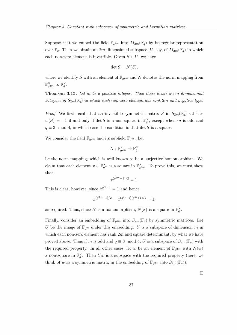
Theorem 3.15. Let m be a positive integer. Then there exists an m-dimensional
subspace of S2m(Fq) in which each non-zero element has rank 2m and negative type.
Proof. We first recall that an invertible symmetric matrix S in S2m(Fq) satisfies
w(S) = −1 if and only if detS is a non-square in F×q , except when m is odd and
q ≡ 3 mod 4, in which case the condition is that detS is a square.
We consider the field Fq2m and its subfield Fqm . Let
N : F×q2m→ F×q
be the norm mapping, which is well known to be a surjective homomorphism. We
claim that each element x ∈ F×qm is a square in F×q2m
. To prove this, we must show
that
x(q2m−1)/2 = 1.
This is clear, however, since xqm−1 = 1 and hence
x(q2m−1)/2 = x(qm−1)(qm+1)/2 = 1,
as required. Thus, since N is a homomorphism, N(x) is a square in F×q .
Finally, consider an embedding of Fq2m into S2m(Fq) by symmetric matrices. Let
U be the image of Fqm under this embedding. U is a subspace of dimension m in
which each non-zero element has rank 2m and square determinant, by what we have
proved above. Thus if m is odd and q ≡ 3 mod 4, U is a subspace of S2m(Fq) with
the required property. In all other cases, let w be an element of Fq2m with N(w)
a non-square in F×q . Then Uw is a subspace with the required property (here, we
think of w as a symmetric matrix in the embedding of Fq2m into S2m(Fq)).
37
Chapter 3: Constant rank subspaces of symmetric and hermitian matrices
Hence we have:
Corollary 3.16. Suppose r = 2m is even and q is odd. Then the maximum di-
mension of a constant rank r subspace of Sn(Fq) where every non-zero element has
negative type, is precisely m.
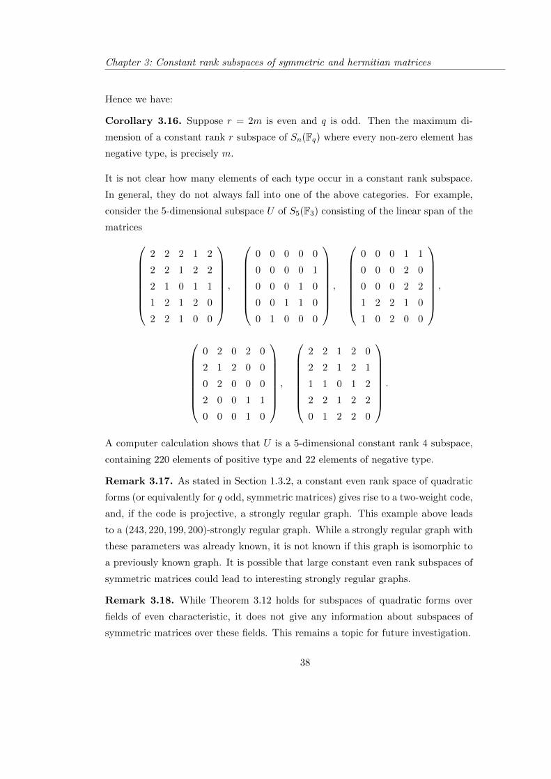
It is not clear how many elements of each type occur in a constant rank subspace.
In general, they do not always fall into one of the above categories. For example,
consider the 5-dimensional subspace U of S5(F3) consisting of the linear span of the
matrices
2 2 2 1 2
2 2 1 2 2
2 1 0 1 1
1 2 1 2 0
2 2 1 0 0
,
0 0 0 0 0
0 0 0 0 1
0 0 0 1 0
0 0 1 1 0
0 1 0 0 0
,
0 0 0 1 1
0 0 0 2 0
0 0 0 2 2
1 2 2 1 0
1 0 2 0 0
,
0 2 0 2 0
2 1 2 0 0
0 2 0 0 0
2 0 0 1 1
0 0 0 1 0
,
2 2 1 2 0
2 2 1 2 1
1 1 0 1 2
2 2 1 2 2
0 1 2 2 0
.
A computer calculation shows that U is a 5-dimensional constant rank 4 subspace,
containing 220 elements of positive type and 22 elements of negative type.
Remark 3.17. As stated in Section 1.3.2, a constant even rank space of quadratic
forms (or equivalently for q odd, symmetric matrices) gives rise to a two-weight code,
and, if the code is projective, a strongly regular graph. This example above leads
to a (243, 220, 199, 200)-strongly regular graph. While a strongly regular graph with
these parameters was already known, it is not known if this graph is isomorphic to
a previously known graph. It is possible that large constant even rank subspaces of
symmetric matrices could lead to interesting strongly regular graphs.
Remark 3.18. While Theorem 3.12 holds for subspaces of quadratic forms over
fields of even characteristic, it does not give any information about subspaces of
symmetric matrices over these fields. This remains a topic for future investigation.
38
Chapter 3: Constant rank subspaces of symmetric and hermitian matrices
3.3 Constant rank 3 spaces of symmetric matrices over
arbitrary fields
In this section we will consider constant odd rank subspaces of symmetric matrices
over different fields, with particular focus on constant rank 3 subspaces.
3.3.1 Constant odd rank subspaces over R
Recall the definition of the order of a polynomial f =∑
i fiyi:
ord(f) := infi | fi 6= 0
Lemma 3.19. Let A be an element of Sn(R), and let char(A) =∑n
i=0 aiyi. Then
rank(A) = n− ord(char(A)).
Proof. It is well known that every real symmetric matrix is similar to a diagonal
matrix. Hence A is similar to diag(b1, b2, . . . , bn) for some bi ∈ R, and rank(A) =
#i | bi 6= 0. Therefore char(A) =∏ni=1(y − bi), and hence the largest power of y
dividing char(A) is #i | bi = 0 = n−rank(A). Hence ord(char(A)) = n−rank(A),
proving the claim.
Hence we have the following result, which is not assumed to be new:
Lemma 3.20. Suppose U is a constant rank r subspace of Sn(R), where r is odd.
Then dim(U) ≤ 1.
Proof. Suppose U has dimension d, and let E1, E2, . . . , Ed be a basis of U . Then
char(
d∑i=1
xiEi) = det(y −d∑i=1
xiEi) = yd +
n∑i=0
fi(x1, x2, . . . , xd)yn−i
where fi is a homogeneous polynomial of degree i in R[x1, x2, . . . , xd]. By Lemma
3.19, fi ≡ 0 for i ≤ r, and fr has no non-trivial zeros (for otherwise U would contain
elements of rank not equal to r). But it is well known that any homogeneous
polynomial of odd degree in R[x1, x2, . . . , xd] has a non-trivial zero unless d = 1,
proving the result.
39
Chapter 3: Constant rank subspaces of symmetric and hermitian matrices
Note that the same result holds for any real closed field, as the proof only relies
on the fact that every symmetric matrix is diagonalizable, and the fact that every
homogeneous polynomial of odd degree has a non-trivial zero, both of which hold
true for real closed fields.
3.3.2 Constant rank 3 subspaces of symmetric matrices over arbi-
trary fields
It seems reasonable to ask if a constant rank r subspace of symmetric matrices over
an arbitrary field has dimension at most r when r is odd. We have proved this is true
for a finite field, and an application of the Kronecker pair theory, discussed below,
shows that over an algebraically closed field, the maximum dimension of an odd
constant rank subspace of symmetric matrices is 1. As an indication that a general
result for all fields might be true, we shall present a proof that, over an arbitrary
field, the maximum dimension of a constant rank 3 subspace of symmetric matrices
is 3.
Let V be a finite dimensional vector space over the field F and let f and g be
symmetric bilinear forms defined on V × V . A basic result in the theory of bilinear
forms, due essentially to Kronecker, shows that there is a decomposition
V = V1 ⊥ V2 ⊥ V3
of V into subspaces V1, V2 and V3. This decomposition is orthogonal with respect
to both f and g: that is, f(vi, vj) = 0 for all vi ∈ Vi 6= Vj 3 vj , and the same holds
true for g. See for example [71], Theorem 3.1.
We may choose the notation so that f is non-degenerate on V1, g is non-degenerate
on V2, and V3 is the orthogonal direct sum (with respect to f and g) of basic singular
subspaces. We allow the possibility that any of the Vi is a zero subspace and also
that g is non-degenerate on V1, or f is non-degenerate on V2.
A basic singular subspace U , say, with respect to f and g, has odd dimension, 2k+1,
say, and the restriction of each of f and g to U × U has even rank 2k. In fact, the
subspace spanned by the restrictions of f and g forms a constant rank 2k subspace.
40
Chapter 3: Constant rank subspaces of symmetric and hermitian matrices
Hence the restrictions of f and g to the subspace V3 above span a constant rank 2s
subspace for some s.
If f and g each have rank r, then the restrictions of f and g to V1 ⊥ V2 each have
rank r − 2s. If s = 0, then V3 is clearly contained in the radical of both f and
g.
We wish to show that if f and g span a constant rank 3 subspace, then we must
have s = 0 and dim(V3) = n− 3, and hence f and g have the same radical.
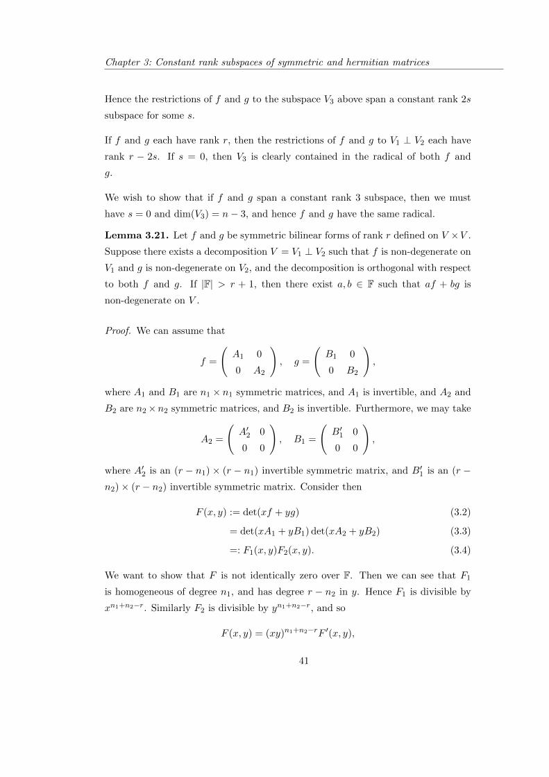
Lemma 3.21. Let f and g be symmetric bilinear forms of rank r defined on V ×V .
Suppose there exists a decomposition V = V1 ⊥ V2 such that f is non-degenerate on
V1 and g is non-degenerate on V2, and the decomposition is orthogonal with respect
to both f and g. If |F| > r + 1, then there exist a, b ∈ F such that af + bg is
non-degenerate on V .
Proof. We can assume that
f =
(A1 0
0 A2
), g =
(B1 0
0 B2
),
where A1 and B1 are n1 × n1 symmetric matrices, and A1 is invertible, and A2 and
B2 are n2×n2 symmetric matrices, and B2 is invertible. Furthermore, we may take
A2 =
(A′2 0
0 0
), B1 =
(B′1 0
0 0
),
where A′2 is an (r − n1) × (r − n1) invertible symmetric matrix, and B′1 is an (r −n2)× (r − n2) invertible symmetric matrix. Consider then
F (x, y) := det(xf + yg) (3.2)
= det(xA1 + yB1) det(xA2 + yB2) (3.3)
=: F1(x, y)F2(x, y). (3.4)
We want to show that F is not identically zero over F. Then we can see that F1
is homogeneous of degree n1, and has degree r − n2 in y. Hence F1 is divisible by
xn1+n2−r. Similarly F2 is divisible by yn1+n2−r, and so
F (x, y) = (xy)n1+n2−rF ′(x, y),
41
Chapter 3: Constant rank subspaces of symmetric and hermitian matrices
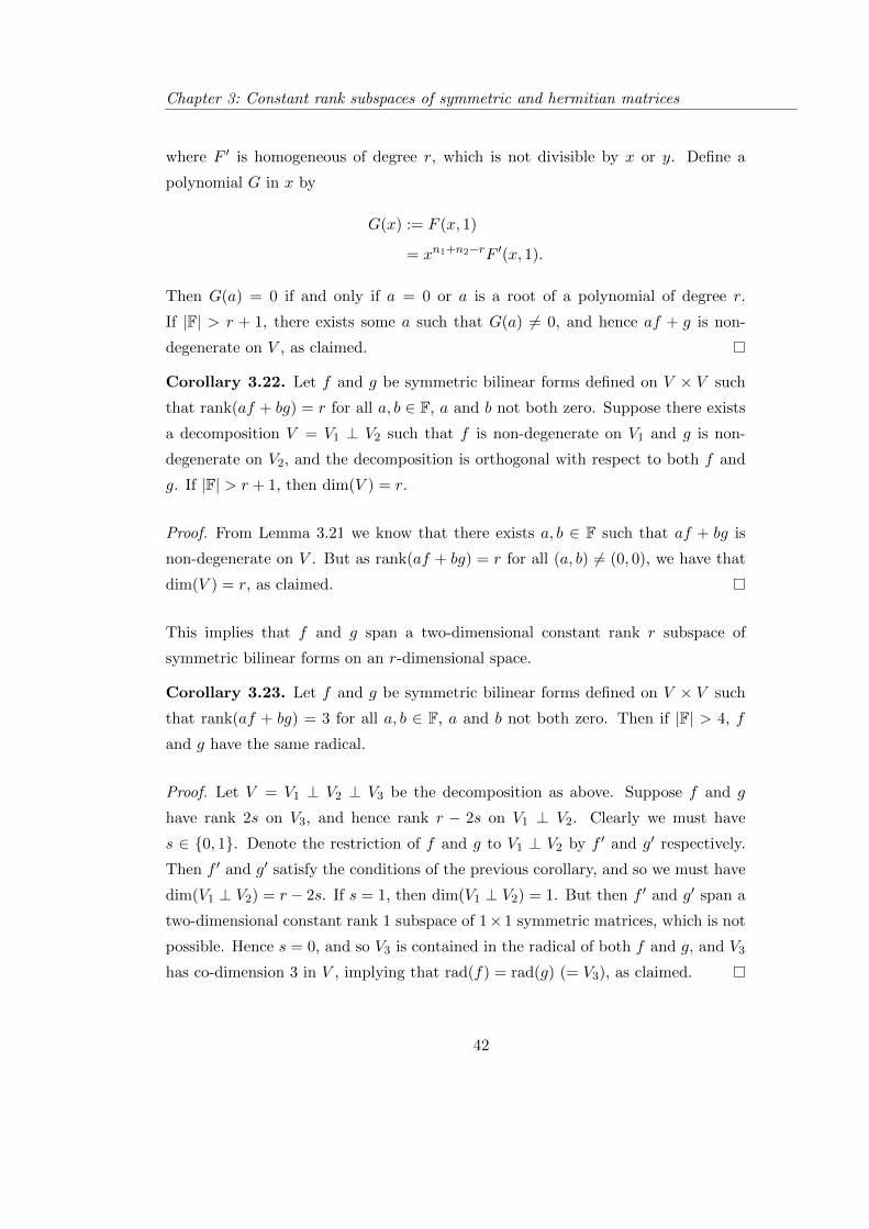
where F ′ is homogeneous of degree r, which is not divisible by x or y. Define a
polynomial G in x by
G(x) := F (x, 1)
= xn1+n2−rF ′(x, 1).
Then G(a) = 0 if and only if a = 0 or a is a root of a polynomial of degree r.
If |F| > r + 1, there exists some a such that G(a) 6= 0, and hence af + g is non-
degenerate on V , as claimed.
Corollary 3.22. Let f and g be symmetric bilinear forms defined on V × V such
that rank(af + bg) = r for all a, b ∈ F, a and b not both zero. Suppose there exists
a decomposition V = V1 ⊥ V2 such that f is non-degenerate on V1 and g is non-
degenerate on V2, and the decomposition is orthogonal with respect to both f and
g. If |F| > r + 1, then dim(V ) = r.
Proof. From Lemma 3.21 we know that there exists a, b ∈ F such that af + bg is
non-degenerate on V . But as rank(af + bg) = r for all (a, b) 6= (0, 0), we have that
dim(V ) = r, as claimed.
This implies that f and g span a two-dimensional constant rank r subspace of
symmetric bilinear forms on an r-dimensional space.
Corollary 3.23. Let f and g be symmetric bilinear forms defined on V × V such
that rank(af + bg) = 3 for all a, b ∈ F, a and b not both zero. Then if |F| > 4, f
and g have the same radical.
Proof. Let V = V1 ⊥ V2 ⊥ V3 be the decomposition as above. Suppose f and g
have rank 2s on V3, and hence rank r − 2s on V1 ⊥ V2. Clearly we must have
s ∈ 0, 1. Denote the restriction of f and g to V1 ⊥ V2 by f ′ and g′ respectively.
Then f ′ and g′ satisfy the conditions of the previous corollary, and so we must have
dim(V1 ⊥ V2) = r − 2s. If s = 1, then dim(V1 ⊥ V2) = 1. But then f ′ and g′ span a
two-dimensional constant rank 1 subspace of 1× 1 symmetric matrices, which is not
possible. Hence s = 0, and so V3 is contained in the radical of both f and g, and V3
has co-dimension 3 in V , implying that rad(f) = rad(g) (= V3), as claimed.
42
Chapter 3: Constant rank subspaces of symmetric and hermitian matrices
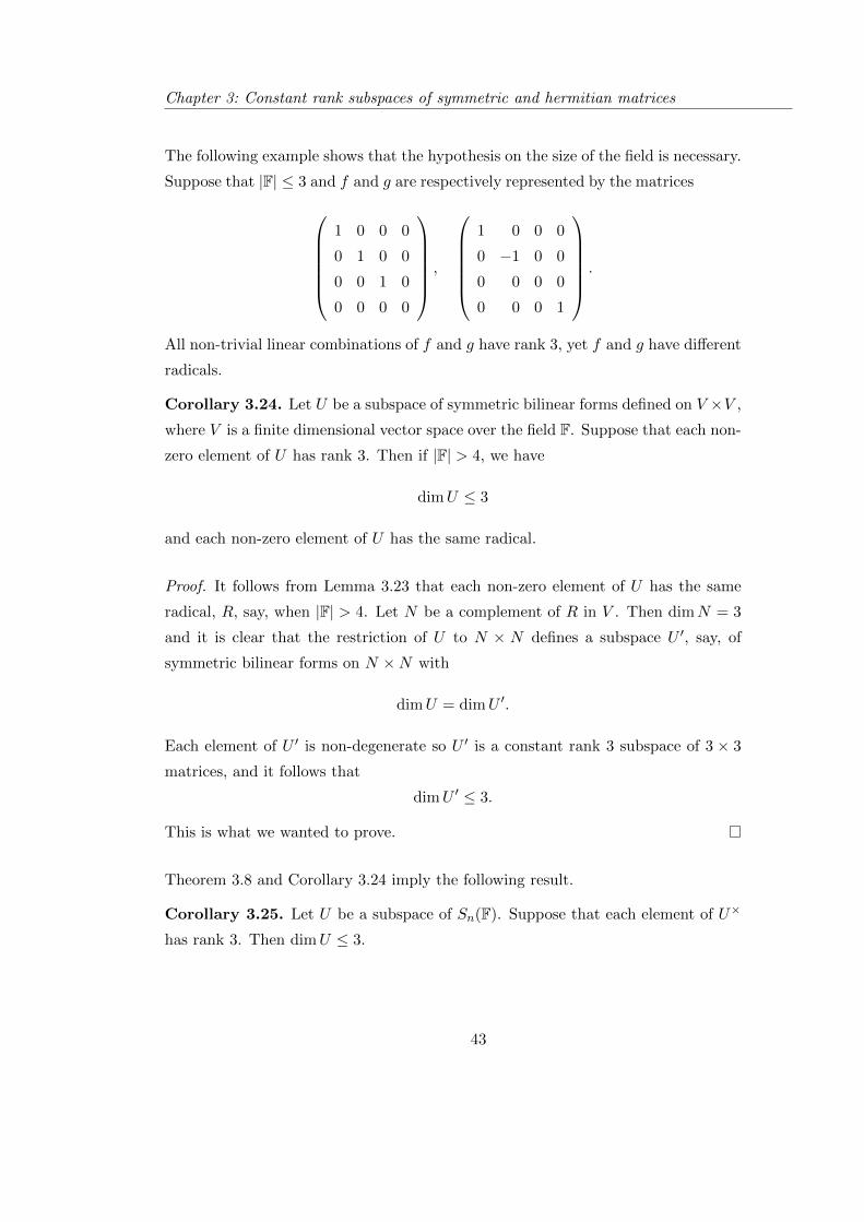
The following example shows that the hypothesis on the size of the field is necessary.
Suppose that |F| ≤ 3 and f and g are respectively represented by the matrices
1 0 0 0
0 1 0 0
0 0 1 0
0 0 0 0
,
1 0 0 0
0 −1 0 0
0 0 0 0
0 0 0 1
.
All non-trivial linear combinations of f and g have rank 3, yet f and g have different
radicals.
Corollary 3.24. Let U be a subspace of symmetric bilinear forms defined on V ×V ,
where V is a finite dimensional vector space over the field F. Suppose that each non-
zero element of U has rank 3. Then if |F| > 4, we have
dimU ≤ 3
and each non-zero element of U has the same radical.
Proof. It follows from Lemma 3.23 that each non-zero element of U has the same
radical, R, say, when |F| > 4. Let N be a complement of R in V . Then dimN = 3
and it is clear that the restriction of U to N × N defines a subspace U ′, say, of
symmetric bilinear forms on N ×N with
dimU = dimU ′.
Each element of U ′ is non-degenerate so U ′ is a constant rank 3 subspace of 3 × 3
matrices, and it follows that
dimU ′ ≤ 3.
This is what we wanted to prove.
Theorem 3.8 and Corollary 3.24 imply the following result.
Corollary 3.25. Let U be a subspace of Sn(F). Suppose that each element of U×
has rank 3. Then dimU ≤ 3.
43
Chapter 3: Constant rank subspaces of symmetric and hermitian matrices
Remark 3.26. In this chapter we have seen that the dimension of a constant rank
3 subspace of Sn(F) is at most 3 for any field F, and also that the dimension of a
constant rank r subspace of Sn(Fq) at most r for any odd r and any finite field Fq.This suggests that result may hold true for any odd r and any field F. However, this
question remains open at this time.
44
Chapter 4
Primitive elements in finite
semifields
In this chapter, we prove the existence of left and right primitive elements in semi-
fields of prime degree over their centre Fq, for q large enough. For this chapter, by
semifield we will always mean finite semifield.
4.1 Primitive elements
Let S be a (pre)semifield n-dimensional over Fq, and a an element of S. For this
chapter we will denote multiplication in S by juxtaposition. We recursively define
the left powers of a by
a(1 = a;
a(i = aa(i−1
for all i > 1. We define the right powers ai) of a similarly. The left and right powers
do not coincide in general.
Definition 4.1. A (pre)semifield S is said to be left primitive if there exists some
a ∈ S such that
S× = a(i : i = 1, . . . , qn−1.
45
Chapter 4: Primitive elements in finite semifields
If such an a exists, we say that a is a left primitive element of S.
We define right primitive similarly.
It is well known that every finite field is left and right primitive ([54], Theorem
2.8). Wene [73] considered the existence of primitive elements of finite semifields,
and showed that they exist in many small semifields. Rua [64] showed that Knuth’s
binary semifield [47] of order 32 does not contain a left or right primitive element.
Knuth’s binary semifields consist of elements of the field Fqn for q even, n odd, with
multiplication defined by
x ? y = xy + (Tr(x)y + Tr(y)x)2.
(Note: for q = 2, n up to 23, all others have primitive elements by computer
calculation.)
Rua and Hentzel [33] showed that for order 32 and 64 there exist semifields which
are left primitive but not right primitive (and vice-versa), and also semifields which
are neither left nor right primitive. No other examples of non-primitive semifields
are known.
In this chapter we will prove the following theorem:
Theorem 4.2. Let S be a semifield, n-dimensional over its centre Fq. Then
(a) if n = 3, for any q, S is both left and right primitive;
(b) if n is prime and q is large enough, S is both left and right primitive.
4.1.1 Primitive elements as invertible matrices
Let S be a (pre)semifield n-dimensional over its centre Fq. We saw in section 2.2
that the set of endomorphisms of left (resp. right) multiplication LS (resp. RS) can
be represented as an n-dimensional constant rank n subspace of Mn(Fq).
Given a matrix A ∈Mn(Fq), the characteristic polynomial of A is defined as
char(A) := det(yI −A) ∈ Fq[y].
46
Chapter 4: Primitive elements in finite semifields
Let Fq(A) denote the Fq-subspace of Mn(Fq) spanned by the powers of A. Then it
is well known ([54] Section 2.5) that
• Fq(A) is a field isomorphic to Fqn if and only if char(A) is irreducible.
• A is a primitive element of Fq(A) if and only if char(A) is primitive.
Hence char(A) is primitive if and only if Ai 6= Aj for 0 ≤ i < j < qn − 1.
We can exploit this using the following important lemma. An alternative proof of
the result can be found in [33].
Lemma 4.3. Let S be a (pre)semifield. Then x is left primitive if and only if Lx
has primitive characteristic polynomial. Similarly, x is right primitive if and only if
Rx has primitive characteristic polynomial over Fq.
Proof. By definition,
x(i = Li−1x x.
Then for any 0 < i < j ≤ qn−1, we have x(i = x(j if and only if (Li−1x −Lj−1
x )x = 0.
Suppose x is left primitive in S. Then Li−1x 6= Lj−1
x for 0 < i < j ≤ qn − 1. Hence
Lx has primitive characteristic polynomial.
Conversely, suppose Lx has primitive characteristic polynomial. Then (Li−1x −Lj−1
x )
is an invertible matrix for 0 < i < j ≤ qn − 1. Hence (Li−1x − Lj−1
x )x 6= 0, and so
x(i 6= x(j for 0 < i < j ≤ qn − 1, implying x is left primitive and thus proving the
claim.
The proof for right primitive elements is similar.
For the binary semifield of order 32 described above, one can check that the set of
characteristic polynomials is given by char(Lx) = y5 + y+ 1, y5 + y4 + y+ 1, y5 +
y4 + 1, none of which is primitive, as expected.
Note that if a (pre)semifield S has a left identity element, i.e. an element e such
that ex = x for all x, if and only if I ∈ LS, where I denotes the identity matrix.
Similarly, S has a right identity element if and only if I ∈ RS.
47
Chapter 4: Primitive elements in finite semifields
Hence to prove that every semifield of prime dimension n over its centre Fq contains a
left and right primitive element, it suffices to show that every n-dimensional constant
rank n subspace of Mn(Fq) containing the identity matrix has an element with
primitive characteristic polynomal.
4.1.2 Homogeneous polynomials over finite fields
In this section, we investigate certain homogeneous polynomials defined in terms
of n-dimensional constant rank n subspaces of Mn(Fq). We begin with a general
definition.
Let F be a field, K be an extension field of F, and let g ∈ K[x1, . . . , xn] be a
polynomial with coefficients in K. Let σ be an automorphism of K fixing F. Then
we let gσ denote the polynomial obtained by applying σ to each coefficient of g.
Definition 4.4. Let K be a cyclic extension of degree n of the field F and let σ
generate the Galois group of K over F. Let f be a non-zero homogeneous polynomial
of degree n in F[x1, . . . , xn]. We say that f is a norm form (with respect to K) if
there exists a basis a1, . . . , an for K over F with
f = ggσ · · · gσn−1,
where
g = a1x1 + · · ·+ anxn ∈ K[x1, . . . , xn].
Suppose that f is a norm form, as above, and the coefficient of xn1 in f is 1. Then
it follows that
1 = a1aσ1 · · · aσ
n−1
1 .
We set
bi = a−11 ai, 1 ≤ i ≤ n.
It is clear that b1 = 1, b2, . . . , bn is a basis for K over F and we may write
f = hhσ · · ·hσn−1,
48
Chapter 4: Primitive elements in finite semifields
where
h = x1 + b2x2 + · · ·+ bnxn.
Thus, under the given hypothesis that the coefficient of xn1 in f is 1, we may represent
the norm form f as a product of Galois conjugate linear polynomials in which the
coefficient of x1 in each is 1.
Note that when we state that f ∈ Fq[x1, . . . , xn] is a norm form of degree n, it
can only be such with respect to Fqn and then we may take σ to be the Frobenius
automorphism λ→ λq of Fqn .
4.1.3 Associated polynomial of semifields
Let U be an n-dimensional constant rank n subspace of Mn(Fq), containing the
identity. Let B = E1, . . . , En be an ordered Fq-basis for U . We know from
Section 2.2 that every such U is the semifield spread set LS of some (pre)semifield
S.
Definition 4.5. Let U and B be as above. Then the associated polynomial of U
with respect to B is the polynomial given by
fU,B(x1, x2, . . . , xn) := det(x1E1 + · · ·+ xnEn).
If we use a different basis B1, say, of U , the corresponding polynomial fU,B1 is
obtained from fU,B by making an invertible linear transformation on the variables
and is thus an equivalent polynomial.
It follows that such properties of the associated polynomials as being irreducible
or a norm form are independent of the choice of basis and depend only on the
subspace.
By abuse of language, we shall henceforth talk of the associated polynomial of U to
be that obtained for an arbitrary choice of ordered basis B in which the first basis
element E1 is the identity matrix and we shall write fU in place of fU,B.
We note the following properties of fU .
49
Chapter 4: Primitive elements in finite semifields
(1) fU is a homogeneous polynomial of degree n.
(2) fU has no non-trivial zeros over Fq, as all non-zero elements of U are invertible.
(3) The coefficient of xn1 is 1 (since E1 = I).
(4) If X = λ1E1 + λ2E2 + . . . + λnEn, λi ∈ Fq, and char(X) is the characteristic
polynomial of X, then
char(X) = det(yI −X) = fU (y − λ1,−λ2, . . . ,−λn) ∈ Fq[y].
Following the notation introduced in Section 2.2, let
LFqn = Lz | z ∈ Fqn
be the semifield spread set of Fqn , an n-dimensional subspace of Mn(Fq). Given
z ∈ Fqn , the eigenvalues of Lz are
z, zq, . . . , zqn−1
and consequently the characteristic polynomial of Lz is
n−1∏i=0
(y − zqi).
Theorem 4.6. Let U be an n-dimensional constant rank n subspace of Mn(Fq),containing the identity matrix. Let E1 = I, . . . , En be an ordered Fq-basis for U
and let fU be the associated polynomial of U with respect to this basis. Suppose that
fU is a norm form, with
f = ggσ · · · gσn−1,
where g = x1 + a2x2 + · · · + anxn and 1, a2, . . . , an is an Fq-basis for Fqn. Given
elements λ1, . . . , λn of Fq, let
A = λ1E1 + λ2E2 + · · ·+ λnEn, z = λ1 + λ2a2 + · · ·+ λnan
be corresponding elements in U and Fqn, respectively. Then A and Lz have the same
characteristic polynomial.
50

Chapter 4: Primitive elements in finite semifields
Proof. By property 4, after Definition 4.5 above,
char(A) = det(yI −A) = fU (y − λ1,−λ2, . . . ,−λn)
=
n−1∏i=0
(y − λ1 − λ2a2 − . . .− λnan)σi
=
n−1∏i=0
(y − z)σi =
n−1∏i=0
(y − zqi).
As we observed earlier, this is the characteristic polynomial of Lz.
Corollary 4.7. Let U be an n-dimensional constant rank n subspace of Mn(Fq),containing the identity matrix. Suppose that the associated polynomial fU is a norm
form. Then each monic irreducible polynomial of degree n in Fq[y] occurs as the
characteristic polynomial of exactly n elements of U .
Hence we have the following immediate consequence of Corollary 4.7 and Lemma
4.3:
Corollary 4.8. Let S be a semifield n-dimensional over Fq. Suppose that the
associated polynomial fLS is a norm form. Then S contains a left primitive element.
Similarly, if fRS is a norm form, then S contains a right primitive element.
4.2 Primitive element theorems
We now apply some known results on norm forms to obtain the main results of this
chapter on primitive elements.
Recall the definition of a generalized twisted field GT(Fqn , k,m, γ) from Definition
2.3. Menichetti ([56], Corollaries 29,32) proved the following theorem:
Theorem 4.9. Let S be a semifield n-dimensional over Fq. Then fLS (resp. fRS) is
a norm form if and only if S is isotopic to a generalized twisted field GT(Fqn , k,m, γ)
for gcd(n, k) = gcd(n,m).
Hence Theorem 4.9 and Corollary 4.8 give us the following theorem:
51
Chapter 4: Primitive elements in finite semifields
Theorem 4.10. Let S be a generalized twisted field GT(Fqn , k,m, γ), where gcd(n, k) =
gcd(n,m). Then S contains both a left and right primitive element.
Remark 4.11. Note that our theorem does not apply to all twisted fields. However,
this does not preclude the possibility that all twisted fields contain left and right
primitive elements.
Remark 4.12. Rua proved the above theorem for n = 3 in [64], by explicitly con-
sidering the multiplication in a twisted field. Our above proof does not require any
knowledge of the multiplication, as it depends only on the fact that the associated
polynomial is a norm form.
For some values of q and n, all semifields of size qn with centre Fq have associated
polynomials which are norm forms, as shown by Menichetti, and hence are both left
and right primitive. We will discuss these cases now, beginning with the well known
Lang-Weil bound :
Theorem 4.13 (Lang-Weil). Let f be an absolutely irreducible homogeneous poly-
nomial in Fq[x1, . . . , xn] of degree d. Let N be the number of zeros of f over Fq.Then N satisfies
|N − qn−1| ≤ (d− 1)(d− 2)qn−32 + Cqn−2
for some C which does not depend on q.
When originally proved, the Lang-Weil theorem, [50], was ineffective, as explicit
bounds for C were not available. More recently, explicit bounds for C have been
proven. See, for example, [30]. As far as we know, the best bound currently available
was proved by Cafure and Matera, [9], Theorem 5.2.
Theorem 4.14 (Cafure and Matera). Let f be as above. Then
|N − qn−1| ≤ (d− 1)(d− 2)qn−32 + 5d
133 qn−2
Hence if q is large enough, a homogeneous polynomial f of degree n in Fq[x1, . . . , xn]
which has no non-trivial zeroes cannot be absolutely irreducible. If n is prime, this
implies that f must be a norm form. Here “q is large enough” means that q satisfies
the equation
qn−1 − 1 > (n− 1)(n− 2)qn−32 + 5n
133 qn−2.
52
Chapter 4: Primitive elements in finite semifields
The above sketches the proof of the following theorem:
Theorem 4.15. Let f be a homogeneous polynomial of degree n in Fq[x1, . . . , xn].
Suppose f has no non-trivial zero in Fq. Then
(a) if n = 3, for any q, f is a norm form;
(b) if n is prime and q is large enough, f is a norm form.
Case (a) was essentially known to Dickson, [24], whose proof was later corrected by
Carlitz, [11]. Case (b) is due to [56], Proposition 17 (where the theorem is stated
in terms of hypersurfaces in projective spaces). Hence Theorem 4.15 and Corollary
4.8 give us:
Theorem 4.16. Let S be a semifield, n-dimensional over its centre Fq. Then
(a) if n = 3, for any q, S is both left and right primitive;
(b) if n is prime and q is large enough, S is both left and right primitive.
Remark 4.17. As an example, if we take n = 5, the condition “q large enough”
becomes q > 6296, i.e. any semifield 5-dimensional over its centre Fq for q > 6296
has both a left and right primitive element. For q < 6296, we only know that the
theorem does not hold for q = 2, and does hold for q = 3.
Remark 4.18. Note that Corollary 4.7 implies that if the associated polynomial
of a semifield S which is n-dimensional over its centre Fq is a norm form, then
every monic irreducible polynomial of degree dividing n occurs as the characteristic
polynomial of an element of LS.
However, this is not a necessary condition for a semifield to be left primitive. For
example, Knuth’s binary semifield S of order 27 contains left (and right) primitive
elements, but not every irreducible polynomial of degree 7 over F2 occurs as the
characteristic polynomial of an element of LS. Furthermore, the LS contains (non-
identity) elements whose characteristic polynomial is not irreducible.
Remark 4.19. It is well known that every finite field contains a primitive element.
Little is known about the existence of primitive elements in other families of semi-
fields. See for example [13], [73].
53
Chapter 5
Semifields from
skew-polynomial rings
In this chapter we will introduce a particular construction for semifields using skew-
polynomial rings. We will show that these are isotopic to cyclic semifields as defined
by Jha and Johnson in [40], and use this representation to obtain new results. We
will also discuss this construction over arbitrary fields, and show how it is connected
to some classical constructions of algebras.
In this chapter F will denote a field, K an extension field of F of degree n, σ an
F-automorphism of K fixing precisely F, and V a vector space of dimension d over
K (and hence dimension nd over F).
5.1 Skew-polynomial rings
Let F be a field, K an extension field, σ an F-automorphism of K. We define a
σ-derivation to be an F-linear map δ : K→ K such that
(ab)δ = aσbδ + aδb
for all a, b ∈ K. The following definition is due to Ore [61]:
54
Chapter 5: Semifields from skew-polynomial rings
Definition 5.1. The skew polynomial ring R = K[t;σ, δ] is defined to be the set
of polynomials in t with coefficients in K, where addition is defined termwise, and
multiplication is defined by ta = aσt+ aδ for all a ∈ K.
Note that the definition in [61] actually allows the coefficient ring K to be a division
ring rather than a field. However, for the purposes of this work we will restrict to
the case where K is a field.
Furthermore, we will restrict to the case where δ = 0, because of the following
theorem of Jacobson [38] Prop 1.2.20:
Theorem 5.2. Let R = K[t;σ, δ] be a skew-polynomial ring over a field K, and
suppose σ 6= id. Then R is isomorphic to K[t;σ′, 0] for some σ′.
We will denote K[t;σ, 0] by K[t;σ]. We will denote the fixed field of σ by F, and the
order of σ by n. We define degree in the usual way, and say that an element f is
irreducible in R if there do not exist any a, b ∈ R with deg(a), deg(b) < deg(f) such
that f = ab. The following important properties of skew-polynomial rings will be
needed in this chapter:
Theorem 5.3 (Ore [61]). Let R = K[t;σ] be a skew-polynomial ring. Then
1. multiplication in R is associative and R satisfies both distributive laws;
2. multiplication in R is not commutative unless σ is the identity automorphism;
3. R is left- and right-Euclidean;
4. R is a left- and right-principal ideal domain;
5. the centre of R is F[tn;σ] ' F[y], where F is the fixed field of σ and the
isomorphism maps tn to y;
6. if f1, f2, . . . , fr, g1, g2, . . . , gs are irreducible elements of R, and
f1f2 . . . fr = g1g2 . . . gs
then r = s and there is a permutation π ∈ Sr such that deg(fi) = deg(gπ(i))
for all i.
55
Chapter 5: Semifields from skew-polynomial rings
Note that properties (1),(3),(4) and (6) also hold for R = K[t;σ, δ].
Hence we can define a semifield as follows:
Theorem 5.4. Let V be the vector space consisting of elements of R of degree
strictly less than d. Let f ∈ R be an irreducible of degree d. Define a multiplication
f on V by
a f b := ab mod rf
where juxtaposition denotes multiplication in R, and ‘ mod r’ denotes remainder
on right division by f . Then Sf = (V, f ) is semifield of dimension nd over F.
Proof. This multiplication is well defined, as R is right-Euclidean. We check that Sfhas no zero divisors. Suppose a, b ∈ Sf , and a f b = 0. This implies ∃h ∈ Sf such
that ab = hf . Comparing degrees, part (6) of Theorem 5.3 gives a contradiction
unless a or b is the zero polynomial. The other properties of a semifield are easily
verified. Obviously Sf has dimension d over K, and hence dimension nd over F.
This construction was considered by Ore [60] and Jacobson [35] in order to de-
fine a class of associative algebras, known as cyclic algebras. Though they did not
consider non-associative structures, the fact that the above construction leads to a
multiplication with no zero divisors was essentially known to them. Petit [63] then
explicitly constructed non-associative algebras in this manner. This point will be
further discussed in Section 5.2 below.
Remark 5.5. Note that for any 0 6= α ∈ K, the polynomials f and αf define the
same semifield.
Remark 5.6. Note that defining the multiplication using remainder on left division
by f also defines a semifield. However, in Section 5.1.2 we will show that the
semifields obtained are Knuth derivatives of each other.
For the rest of this chapter we will write mod for modr unless otherwise stated, and
write divides for right divides.
56
Chapter 5: Semifields from skew-polynomial rings
5.1.1 Eigenring and nuclei
Definition 5.7. Let f be an irreducible element of R of degree d. Define the eigen-
ring of f by
E(f) = u ∈ R | deg(u) < d, f divides fu
Theorem 5.8. [63] Let f be a monic irreducible element of R of degree d, and let
Sf be the semifield as defined above. Then
Nr(Sf ) = E(f)
and
E(f) = Sf ⇔ f ∈ Z(R)
where Z(R) denotes the centre of R.
Proof. First we will prove the second assertion. Suppose E(f) = Sf . Let
f =d∑i=0
fiti
where fi ∈ K, and fd = 1 as f is monic. As t ∈ E(f) by assumption, we must have
ft ≡ 0 mod f . But then
ft mod f = ft− tf
=d∑i=0
(fi − fσi )ti
= 0,
implying that fi = fσi for all i, and so fi ∈ F for all i. Now as α ∈ E(f) for all
α ∈ K, we have
fa mod f = fα− ασdf
=d∑i=0
(ασi − ασd)fiti
= 0,
implying that for each i we have fi = 0 or ασi
= ασd
for all a ∈ K. As f is
irreducible, we must have f0 6= 0 (for otherwise t would divide f). Hence if fi 6= 0,
57
Chapter 5: Semifields from skew-polynomial rings
we have ασi
= α for all α ∈ K, and so σi = id. Hence if fi 6= 0 then n divides i.
Therefore f ∈ F[tn;σ] = Z(R), as claimed.
Conversely, if f ∈ Z(R) then clearly fu = uf is divisible by f for all u, and so
E(f) = Sf .
We now show that Nr(Sf ) = E(f). For any a, b, c ∈ F of degree less than d = deg(f)
we can find unique u, v, w, z ∈ R of degree less than d such that
ab = uf + v, and
bc = wf + z,
i.e. a f b = v, b f c = z. Then
(a f b) f c = v f c = vc mod f,
while
a f (b f c) = a f z = az mod f.
But as R is associative, we have that
ufc+ vc = (ab)c = a(bc) = awf + az,
and hence
az = ufc+ vc mod f.
Therefore
(a f b) f c = a f (b f c)⇔ ufc = 0 mod f.
Let c be in the right nucleus. One can choose a, b such that u = 1. Then fc = 0
mod f , implying that c ∈ E(f). Conversely, if c ∈ E(f) then ufc = 0 mod f for
all u, and hence c is in the right nucleus, as claimed.
Hence we get the following corollary:
Corollary 5.9. [63] Sf is associative if and only if f ∈ Z(R).
We will see in Lemma 6.7 that if K is a finite field, then every element of Z(R) is
reducible. This is also implied by the Wedderburn-Dickson theorem, for otherwise
we would obtain a non-commutative finite division algebra. We will see in Section
5.2 however that such elements can exist over infinite fields.
58
Chapter 5: Semifields from skew-polynomial rings
Theorem 5.10. [63] Suppose f is a monic irreducible element of R = K[t;σ] such
that f /∈ Z(R). The left and middle nuclei of Sf are given by
Nl(Sf ) = Nm(Sf ) = (K).1
i.e. they are the set of constant polynomials, and the centre is
Z(Sf ) = (F).1.
Proof. Let a, b, c ∈ R, and u, v, w, z be as defined in the proof of Theorem 5.8. We
saw that (a f b) f c = a f (b f c)⇔ ufc = 0 mod f .
We show that an element is in the left nucleus if and only if it has degree zero. First
suppose a has degree zero. Then for any b, ab has degree strictly less than d, and
hence u = 0 for all b. Therefore ufc = 0 mod f for all b, c, and so a ∈ Nl.
Suppose now deg(a) = r > 0, and let ar be the leading coefficient of a. Let b =1
a−σr
rtd−r. Then ab is monic, and has degree d, and so u = 1. Let c be some element
not in E(f), i.e. fc 6= 0 mod f . We know that such an element exists as f /∈ Z(R).
Then ufc = fc 6= 0 mod f , and so a /∈ Nl.
The proof for Nm is similar.
The centre is a subfield of Nl, and so consists of all constant polynomials which
commute with t. Since ta = aσt for all a ∈ K, the centre is therefore equal to the
fixed field of σ, which is F.
The nuclei of Sf were calculated in a different way by Dempwolff in [20], when he
calculated the nuclei of cyclic semifields, which we will show in Section 5.2.4 to be
equivalent to this construction.
5.1.2 Semifields from different skew-polynomial rings
In this section, we consider the isotopism problem for semifields constructed from
different skew polynomial rings.
59
Chapter 5: Semifields from skew-polynomial rings
Consider the more general skew polynomial ring of the form K[t;σ, δ]. As noted
above, Jacobson showed that if K is a field, then this ring is isomorphic to K[t;σ′]
for some σ′. We will now illustrate this for finite fields.
For any x ∈ K the map
δx : a 7→ x(a− aσ)
is a σ-derivation. It is easily verified that for a finite field, every σ-derivation is of
this form. The following theorem shows, K[t;σ, δx] is isomorphic to K[t;σ] for all x,
and hence the semifields obtained are isotopic.
Theorem 5.11. Let R = K[t;σ] and R′ = K[t;σ, δx] be skew-polynomial rings.
Denote the multiplication in R and R′ by and ′ respectively. Then R and R′ are
isomorphic via the map φ : R→ R′ defined by
a(t) 7→ a(t− x),
where the evaluation of a(t − x) occurs in R′ (i.e. φ(t2) = (t − x) ′ (t − x)). The
map φ is linear and
φ(a b) = φ(a) ′ φ(b)
for all a, b ∈ R
Proof. Clearly by the definition of φ, φ(ti tj) = φ(ti) ′ φ(tj) for all i, j, and
φ(α βti) = φ(α) ′ φ(βti) for all α, β ∈ K and all i. Hence it suffices to show that
φ(t α) = φ(t) ′ φ(α)
for all α ∈ K. Now
φ(t α) = φ(ασt) = φ(ασ) ′ φ(t) = ασ ′ (t− x) = ασt− xασ
while
φ(t) ′ φ(α) = (t− x) ′ α = ασt+ x(α− ασ)− xα = ασt− xασ
and the result holds.
Note that defining the multiplication using remainder on left division by f also
defines a semifield. Denote this semifield by fS, and the multiplication by ‘f’. The
following theorems show that the semifields obtained are Knuth derivatives of each
other.
60
Chapter 5: Semifields from skew-polynomial rings
Theorem 5.12. Let R = K[t;σ] and R′′ = K[t;σ−1] be skew-polynomial rings.
Denote the multiplication in R and R′′ by and ′′ respectively. Then R and R′ are
anti-isomorphic via the map ψ : R→ R′ defined by
ψ(∑
aiti)
=∑
aσ−ii ti,
i.e.
ψ(a b) = ψ(b) ′′ ψ(a)
Proof. For any a, b,
ψ(a b) = ψ
∑i,j
aibσi
j ti+j
=∑i,j
aσ−i−ji (bσ
i
j )σ−i−j
ti+j
=∑i,j
(bσ−jj )(aσ
−ii )σ
−jti+j
=∑i,j
ψ(b)j(ψ(a)i)σ−j ti+j
= ψ(b) ′′ ψ(a),
as claimed.
Corollary 5.13. Let R, R′′ and ψ be as above. Let f be irreducible in R. Then
1. ψ(f) is irreducible in R′;
2. If Sf = R mod Rf , and ψ(f)S′′ = R′′ mod ψ(f)R′, then Sf and ψ(f)S′′ are
anti-isomorphic (and hence Knuth derivatives of each other).
Proof. (1) Clear, for if ψ(f) = ψ(a)′′ψ(b), then by the previous theorem, f = ba.
But then a or b must be a unit, and as ψ preserves degrees, ψ(a) or ψ(b) must be a
unit.
(2) We claim that ψ is an anti-isomorphism from Sf to ψ(f)S′′. Clearly ψ is a bijective
linear map. We need to show that
ψ(a f b) = ψ(b)ψ(f) ′′ ψ(a),
61
Chapter 5: Semifields from skew-polynomial rings
where
a f b = a b mod r f, and
ψ(b)ψ(f) ′′ ψ(a) = ψ(b) ′′ ψ(a) mod l ψ(f).
Let a b = u f + v, where deg(v) < d = deg(f). Then using the above theorem we
obtain
ψ(a f b) = ψ(v)
= ψ(a b− u f) = ψ(a b)− ψ(u f)
= ψ(b) ′′ ψ(a)− ψ(f) ′′ ψ(u) = ψ(b) ′′ ψ(a) mod l ψ(f)
= ψ(b)ψ(f) ′′ ψ(a),
as claimed.
Hence we have
K(Sf ) : f irreducible in K[t;σ] = K(fS) : f irreducible in K[t;σ−1].
Remark 5.14. It is not clear when different skew polynomial rings R = K[t;σ] and
R′ = K[t;σ′] define isotopic semifields. It is a necessary condition that σ and σ′ have
the same order.
We will see in Section 5.2.4 that a result of Kantor and Liebler implies that every
semifield Sf for f ∈ K[t;σ] is isotopic to Sf for some f ∈ K[t;σ−1]. Hence we have
that
[Sf ] : f irreducible in K[t;σ] = [Sf ] : f irreducible in K[t;σ−1].
Therefore combining this with the above result, we have
K(Sf ) : f irreducible in K[t;σ] = K(fS) : f irreducible in K[t;σ].
5.2 Connections with known constructions
5.2.1 Knuth semifields
We will now explicitly calculate the multiplication in Sf when f has degree 2
for illustrative purposes and for later comparison with previously known construc-
62
Chapter 5: Semifields from skew-polynomial rings
tions.
Suppose f ∈ K[t;σ] has degree d. Then it has been shown by Ore ([62] Theorem
3) that f =∑
i fiti has a linear right divisor if and only if there exists an element
α ∈ K such that
f0 + f1α+ f2α1+σ + f3α
1+σ+σ2+ . . .+ fdα
1+σ+...+σd−1= 0.
Hence if f = t2 − xt− y, then f is irreducible if and only if
ασ+1 − xα− y = 0
has no solutions α ∈ K.
Suppose now f = t2 − xt − y is irreducible. Write elements a + bt ∈ Sf as a tuple
(a, b) ∈ K2. Then
(a+ bt)(c+ dt) = ac+ (bcσ + ad)t+ bdσt2
= ac+ (bcσ + ad)t+ bdσ(f + xt+ y)
≡ (ac+ xbdσ) + (bcσ + ad+ ybdσ)t mod rf
Hence
(a, b) f (c, d) = (ac+ xbdσ, ad+ bcσ + ybdσ). (5.1)
Similarly, if we let fS denote the semifield obtained by taking remainder on left
division by f , then
(a, b)f (c, d) = (ac+ xbσ−1dσ−2, aσd+ bc+ ybdσ
−1). (5.2)
In [46], section 7.4, Knuth defined four classes of semifields two-dimensional over K.
We will denote them by (K1)− (K4). The multiplications are defined by
(K1) (ac+ xbσdσ−2, bc+ aσd+ ybσdσ
−1)
(K2) (ac+ xbσd, bc+ aσd+ ybσd)
(K3) (ac+ xbσ−1dσ−2, bc+ aσd+ ybdσ
−1)
(K4) (ac+ xbσ−1d, bc+ aσd+ ybd)
where we assume that ασ+1 + xα− y = 0 has no solutions α ∈ K.
Then comparing these with equations 5.1 and 5.2 gives us:
63
Chapter 5: Semifields from skew-polynomial rings
Theorem 5.15. Let f be an irreducible polynomial of degree 2 in K[t;σ]. Then
• Sopf is a semifield of type (K2).
• fS is a semifield of type (K3).
Note that the condition that ασ+1 +xα−y = 0 has no solutions α ∈ K is equivalent
to the condition that f ′ = t2 + xt− y is irreducible. But as we will see in the next
section, the map t 7→ −t is an isomorphism of K[t;σ], and so f = t2 − xt − y is
irreducible if and only if f ′ is irreducible.
Hence we can see that these two families can be thought of as a special case of
the construction using skew-polynomial rings. Knuth implicitly showed that these
families are Knuth derivatives of each other, as noted in [4]. We see from Section
5.1.2 that that this is a special case of the more general fact that the families Sf :
f irreducible and fS : f irreducible are Knuth derivatives of each other.
5.2.2 Cyclic algebras
Given a field K, an automorphism σ of K with fixed field F, and a non-zero element
γ of F, we define the cyclic algebra (K, σ, γ) as follows: Let e0, e1, . . . , ed−1 be a
K-basis for the vector space Kd. Define a multiplication on Kd by
eiα = ασiei
for all α ∈ K, and
eiej =
ei+j if i+ j < d
γei+j−d if i+ j ≥ d
As can be seen in ([38], Section 1.4), if we identify ei ↔ ti, then
(K, σ, γ) ' K[t;σ]
〈tn − γ〉' Stn−γ .
Hence this construction is a special case of the above construction using skew-
polynomial rings. As shown in Theorem 5.8, given a skew-polynomial ring R and
an element f , the algebra Sf is associative if and only if f is in the centre of R, and
Sf is a division algebra if and only if f is irreducible in R. Hence the cyclic algebra
(K, σ, γ) is always associative, and is a division algebra if and only if f ∈ Z(R). We
64
Chapter 5: Semifields from skew-polynomial rings
will see in Lemma 6.7 that for skew-polynomial rings over finite fields, every central
element is reducible. However, over many fields this is not true, and much study has
been done on the problem of deciding when a cyclic algebra is a division algebra.
Cyclic division algebras have been used in space-time coding, e.g. in [59].
It is not clear whether irreducible elements must exist for all degrees in an arbitrary
skew-polynomial ring. This remains a problem for future research.
5.2.3 Nonassociative analogues of cyclic algebras
Ore and Jacobson, when studying cyclic algebras, each considered structures ob-
tained from the vector space of residue classes of R = K[t;σ] modulo a left ideal
Rf . As they were interested only in associative algebras, they restricted to a sub-
structure, the eigenring E(f). They each proved (in different ways) the following
theorem ([60], p. 242 and [35], p. 201-202):
Theorem 5.16. If f is irreducible in R, then E(f) is a[n associative] division
algebra.
As we have seen in the previous sections, if we choose a specific representative of
each residue class (the unique element of degree less than deg(f)), then the structure
Sf obtained is a non-associative algebra. The theorem then extends to:
Theorem 5.17. If f is irreducible in R, then Sf is a division algebra.
The proof relies only on the theorem of Ore (Theorem 5.3 above). Hence it is perhaps
fair to say that the construction of the semifields Sf was, in essence, known to Ore
and Jacobson.
Petit [63] explicitly constructed the semifields Sf in 1966, and calculated the nuclei.
This work was brought to the author’s attention by W.M. Kantor subsequent to the
original submission of this thesis.
Sandler [68] considered non-associative generalizations of cyclic algebras over finite
fields. These can be seen to be precisely algebras of the form Sf , where f = tn−γ ∈K[t;σ] and γ /∈ F. He showed that this defines a semifield if and only if γ does not
lie in any proper subfield of K.
65
Chapter 5: Semifields from skew-polynomial rings
Jha and Johnson further generalized this by defining cyclic semifields, using the
theory of semilinear transformations. We will now show that these semifields are
precisely the semifields (isotopic to) semifields of the form Sf , f ∈ R.
5.2.4 Equivalence with cyclic semifields
Definition 5.18. A semilinear transformation on a vector space V = Kd is an
additive map T : V → V such that
T (αv) = ασT (v)
for all α ∈ K, v ∈ V , for some σ ∈ Aut(K). The set of invertible semilinear
transformations on V form a group called the general semilinear group, denoted by
ΓL(d,K).
Note that choosing a basis for V gives us
T (v) = A(vσ)
where A is some invertible K-linear transformation from V to itself, σ is an auto-
morphism of K, and vσ is the vector obtained from v by applying the automorphism
σ to each coordinate of v with respect to this basis.
Definition 5.19. An element T of ΓL(d,K) is said to be irreducible if the only
T -invariant subspaces of V are V and 0.
In [40] Jha and Johnson defined a semifield as follows.
Theorem 5.20. Let T be an irreducible element of ΓL(d,K). Fix a K-basis e0, e1, . . . , ed−1of V . Define a multiplication on V by
a b = a(T )b =d−1∑i=0
aiTi(b)
where a =∑d−1
i=0 aiei. Then ST = (V, ) defines a semifield.
We call a semifield ST a cyclic semifield. It is clear that the spread set of endomor-
phisms of left multiplication of ST is given by
LST = d∑i=0
aiTi : ai ∈ K.
66
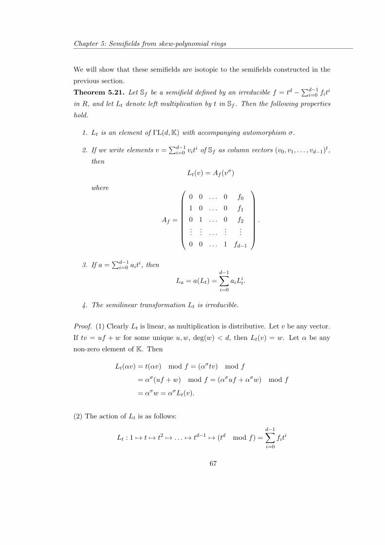
Chapter 5: Semifields from skew-polynomial rings
We will show that these semifields are isotopic to the semifields constructed in the
previous section.
Theorem 5.21. Let Sf be a semifield defined by an irreducible f = td −∑d−1
i=0 fiti
in R, and let Lt denote left multiplication by t in Sf . Then the following properties
hold.
1. Lt is an element of ΓL(d,K) with accompanying automorphism σ.
2. If we write elements v =∑d−1
i=0 viti of Sf as column vectors (v0, v1, . . . , vd−1)t,
then
Lt(v) = Af (vσ)
where
Af =
0 0 . . . 0 f0
1 0 . . . 0 f1
0 1 . . . 0 f2
...... . . .
......
0 0 . . . 1 fd−1
.
3. If a =∑d−1
i=0 aiti, then
La = a(Lt) =d−1∑i=0
aiLit.
4. The semilinear transformation Lt is irreducible.
Proof. (1) Clearly Lt is linear, as multiplication is distributive. Let v be any vector.
If tv = uf + w for some unique u,w, deg(w) < d, then Lt(v) = w. Let α be any
non-zero element of K. Then
Lt(αv) = t(αv) mod f = (ασtv) mod f
= ασ(uf + w) mod f = (ασuf + ασw) mod f
= ασw = ασLt(v).
(2) The action of Lt is as follows:
Lt : 1 7→ t 7→ t2 7→ . . . 7→ td−1 7→ (td mod f) =d−1∑i=0
fiti
67
Chapter 5: Semifields from skew-polynomial rings
and so Lt(v) = Af (vσ) as claimed.
(3) By definition,
La(b) = a f b =
(d−1∑i=0
aiti
)b mod f =
d−1∑i=0
ai(tib mod f) =
d−1∑i=0
aiLti(b)
while
a(Lt)(b) :=
d−1∑i=0
aiLit(b).
Hence it suffices to show that Lit(b) = Lti(b) for all i. Suppose Lit(b) = (tib) mod f
for some i. Let Lit(b) = b′. Then tib = cf + b′ for some c, and
Li+1t (b) = Lt(L
it(b)) = Lt(b
′)
= Lt(tib− cf) = t(tib− cf) mod f
= (ti+1b− tcf) mod f = (ti+1b) mod f
= Lti+1(b).
Hence the result follows by induction.
(4) Let W be a Lt-invariant subspace of V such that 0 < r := dim(W ) < d. Choose
some non-zero w ∈W . Then the set
w,Ltw,L2tw, . . . , L
rtw ⊂W
is linearly dependent. Hence there exist elements a0, a1, . . . , ad in K, not all zero,
such thatd−1∑i=0
ai(Litw) = 0.
Let a =∑d−1
i=0 aiti. Then (
d−1∑i=0
aiLit
)w = a(Lt)w = 0.
By part (3) of this theorem, a(Lt) = La, and so
a f w = 0.
But a f w = 0 implies a = 0 or w = 0, a contradiction. Hence Lt is irreducible.
68
Chapter 5: Semifields from skew-polynomial rings
Corollary 5.22. The spread set of endomorphisms of left multiplication of elements
in Sf is a(Lt) | a ∈ Sf.
The following theorem is an immediate consequence of the definition of ST and
Theorem 5.21.
Theorem 5.23. If f is irreducible in R, and Lt,f denotes the semilinear transfor-
mation v 7→ tv mod f , then Sf = SLt,f .
Kantor and Liebler [44] noted that conjugate semilinear transformations define iso-
topic semifields.
Lemma 5.24. Suppose T = φ−1Uφ for some φ ∈ ΓL(d,K), and let ρ ∈ Aut(K) be
the accompanying automorphism of φ. Let ST = (V, ), SU = (V, ?). Then
φ(a b) = aρ ? φ(b).
Hence to show that
[ST ] = [Sf ],
where T runs through all irreducible elements of ΓL(d,K) and f runs through all
irreducible elements of K[t;σ] of degree d, it suffices to show that T is ΓL(d,K)-
conjugate to Lt,f for some f irreducible of degree d in K[t;σ].
Theorem 5.25. Let T be any irreducible element of ΓL(d,K) with automorphism
σ. Then T is GL(d,K)-conjugate to Lt,f for some f ∈ R = K[t;σ], and hence ST is
isotopic to Sf .
Proof. Identify V with the set of polynomials of degree ≤ d − 1 in R and choose
some non-zero element v ∈ V . Consider the basis
v, Tv, T 2v, . . . , T d−1v,
and define a transformation φ ∈ GL(d,K) by
φ(ti) := T iv,
for i = 0, 1, . . . , d− 1. Then there exist fi ∈ K such that
T dv =
d−1∑i=0
fiTiv.
69
Chapter 5: Semifields from skew-polynomial rings
We claim that
Tφ = φLt,f ,
with
f = td −d−1∑i=0
fiti ∈ R.
It suffices to show that these transformations coincide on ti for all i. Suppose first
that i < d− 1. Then
Tφ(ti) = T (T iv) = T i+1v,
while
φLt,f (ti) = φ(ti+1 mod f) = φ(ti+1) = T i+1v,
as claimed. Suppose now i = d− 1. Then
Tφ(td−1) = T (T d−1v) = T dv =
d−1∑i=0
fiTiv,
while
φLt,f (td−1) = φ(td mod f) = φ
(d−1∑i=0
fiti
)=
d−1∑i=0
fiTiv,
and so
Tφ = φLt,f
as claimed.
Note that the polynomial f depends on the choice of v, and hence T may be ΓL(d,K)-
conjugate to Lt,g for some other g ∈ K[t;σ]. We will see in the Chapter 6 when two
semilinear transformations Lt,g and Lt,f are ΓL(d,K)-conjugate.
Remark 5.26. The following observation of Kantor and Liebler (in [44]), together
with the above theorems, allow us to prove the assertion in Remark 5.14.
If T is an irreducible semilinear transformation with automorphism σ, then T−1
is an irreducible semilinear transformation with automorphism σ−1, and ST and
ST−1 are isotopic. (See [44], Remark 4.1, where the statement is made in terms of
projective planes.)
70
Chapter 5: Semifields from skew-polynomial rings
This implies that every semifield Sf for f ∈ K[t;σ] is isotopic to Sf for some f ∈K[t;σ−1]. In fact it can be shown that f is the reciprocal of f . Hence we have that
[Sf ] : f irreducible in K[t;σ] = [Sf ] : f irreducible in K[t;σ−1].
5.2.5 Quaternion algebras and Cayley-Dickson algebras
In this section we will recall the well-known construction of quaternion algebras
and Cayley-Dickson algebras, and show that they can be constructed using skew-
polynomial rings.
Definition 5.27. Let F be a field with char(F) 6= 2, and let a, b be non-zero elements
of F. Define the quaternion algebra Q(a, b)F to be the set of elements of the form
α+ βi+ γj + δk
for all α, β, γ, δ ∈ F, with multiplication defined by the relations
i2 = a, j2 = b, ij = −ji = k.
Note that these algebras are sometimes denoted in the literature by(a,bF
). These
algebras are generalizations of Hamilton’s quaternions, H = Q(−1,−1)R.
If a is a non-square in F, we see that F(i) = F(√a) is a field extension of F of degree
2. It is easily seen that there exists an automorphism σ on F(i) defined by
(α+ βi)σ = α− βi.
Then we can write elements of Q(a, b)F in the form
λ+ µj,
for λ, µ ∈ F(i). Then the multiplication is determined by
jλ = j(α+ βi)
= αj + βji
= αj − βij
= (α− βi)j
= λσj,
71
Chapter 5: Semifields from skew-polynomial rings
for all λ ∈ F, and j2 = b.
Consider now the skew-polynomial ring R = F(i)[t;σ], and the polynomial f = t2−b.Constructing the division algebra Sf as in Section 5.1, we can see that by identifying
j with t, these two constructions coincide precisely, and so if σ is the automorphism
of F(√a) sending
√a to −
√a then
Q(a, b)F 'F(√a)[t;σ]
〈t2 − b〉= Sf .
Definition 5.28. Let F be a field, and K a separable quadratic field extension of Fwith non-trivial Galois automorphism σ. Let b be a non-zero element of K. Define
a multiplication on K×K by
(α, β)(γ, δ) := (αγ + bδβσ, ασδ + γβ)
for α, β, γ, δ ∈ K. The algebra obtained is called the Cayley-Dickson double of Kwith scalar b, and is denoted by Cay(K, b).
The algebra Cay(K, b) is associative if and only if b ∈ F, as implied by Corollary 5.9.
These were originally defined for b ∈ F, and extended to b ∈ K by Dickson [25]. If
we take K = F(√a), then we have
Cay(K, b) ' Q(a, b)F.
Comparing this definition with equation 5.1, we see that the Cayley-Dickson double
of a field, and hence the quaternion algebras, are special cases of the construction
from skew-polynomial rings.
For the case of Hamilton’s quaternions, we have
H =C[t;σ]
〈t2 + 1〉= St2+1,
where σ denotes complex conjugation.
It can be shown that if R = K[t;σ] is a skew-polynomial ring, then there exists an
anti-automorphism of R if and only if σ2 = 1, and all anti-automorphisms are of the
form ∑akt
k 7→∑
aσ−k+mk (λt)k,
72
Chapter 5: Semifields from skew-polynomial rings
where 0 6= λ ∈ K and m ∈ 0, 1. The proof of this is similar to the proofs of
Theorem 5.12 and Lemma 6.1 in the next chapter, and so is omitted here. If f is
irreducible in R and lies in the centre of R, then the restriction of this map to Sf is
an anti-automorphism of Sf . Choosing m = 1, λ = −1, we see that we obtain the
usual quaternion conjugation: if a = α+ βi ∈ C, b = γ + δi ∈ C, then
(a+ bj) = aσ − bj
= (α+ βi)σ − (γ + δi)j
= α− βi− γj − δij.
Note that the Cayley-Dickson doubling process can also be applied to a division
algebra D. This does not, in general, coincide with residue algebras obtained from
D[t;σ], as the Cayley-Dickson process uses this anti-automorphism above rather
than an automorphism, and the order of multiplication of elements of D do not
match.
73
Chapter 6
Isotopy classes of semifields
from skew-polynomial rings
In this chapter we will consider the problem of deciding when two semifields Sf and
Sg are isotopic. We will then apply these results to obtain an improved upper bound
on the number of isotopy classes over a finite field.
6.1 Isotopy relations
We begin by considering automorphisms of skew-polynomial rings. The following
lemma is not assumed to be new, but a proof is included for lack of convenient
reference.
Lemma 6.1. Let φ be an automorphism of R = K[t;σ], where σ is not the identity
automorphism. Then
φ(f) = fρ(αt)
where ρ ∈ Aut(K) and α ∈ K×.
Proof. As φ is bijective, it preserves the degree of elements of R. Let ρ be the field
automorphism obtained by the restriction of φ to K, and assume φ(t) = αt + β,
74
Chapter 6: Isotopy classes of semifields from skew-polynomial rings
α, β ∈ K, α 6= 0. Choose γ ∈ K such that γσ 6= γ. Computing φ(t)φ(γ) = φ(tγ) =
φ(γσt) = φ(γσ)φ(t), we see that β = 0, and the assertion follows.
Automorphisms of R can be used to define isomorphisms between semifields.
Theorem 6.2. Let f be a monic irreducible of degree d in R. Let φ be an automor-
phism of R. Define g = φ(f). Then Sf and Sg are isomorphic, and
φ(a f b) = φ(a) g φ(b).
Proof. For any a, b ∈ R of degree less than d, there exist unique u, v ∈ R such that
deg(u),deg(v) < d and
ab = uf + v.
Then a f b = v = ab− uf . As φ is an automorphism of R, we have that
φ(a f b) = φ(ab− uf) = φ(a)φ(b)− φ(u)φ(f) = φ(a) g φ(b)
as claimed.
We now consider another type of isotopism between these semifields.
Definition 6.3. Let f and g be monic irreducibles of degree d in R. We say that
f and g are similar if there exists a non-zero element u of R of degree less than d
such that
gu ≡ 0 mod f.
Theorem 6.4. Suppose f and g are similar. Then Sf and Sg are isotopic, and
(a g b)H = a f bH
where bH = b f u, gu ≡ 0 mod f .
Proof. Let a g b = ab− vg. Then
(a g b)H = (ab− vg)H
= (ab− vg)u mod f
= (abu− vgu) mod f
≡ abu mod f,
75
Chapter 6: Isotopy classes of semifields from skew-polynomial rings
as gu ≡ 0 mod f .
Let b f u = bu− wf . Then
a f bH = a f (b f u)
= a f (bu− wf)
= a(bu− wf) mod f
≡ abu mod f,
and the result holds.
In [36] Jacobson investigated when two skew polynomials are similar. In the next
section we will include a proof for skew polynomial rings over finite fields for the
sake of completeness, and because some of the concepts introduced will be of use
later in this chapter for counting isotopy classes.
6.2 Counting isotopy classes for finite semifields
For this section we will assume K = Fqn , F = Fq are finite fields, although some of
the concepts introduced remain valid for arbitrary fields.
Let A(q, n, d) denote the number of isotopy classes of semifields of order qnd defined
by the skew polynomial ring Fqn [t;σ], with
(#Z,#Nl,#Nm,#Nr) = (q, qn, qn, qd),
i.e.
A(q, n, d) := |[Sf ] : f irreducible in Fqn [t;σ], deg(f) = d|.
In this section we will apply the isotopy relations outlined in the previous section to
obtain a new upper bound for A(q, n, d).
Definition 6.5. Let f ∈ R be irreducible of degree d. Define the minimal central
left multiple of f , denoted by mzlm(f), as the monic polynomial of minimal degree
in the centre Z ' Fq[tn;σ] ' Fq[y] that is right-divisible by f .
76
Chapter 6: Isotopy classes of semifields from skew-polynomial rings
In [31] Giesbrecht showed that mzlm(f) exists, is unique, has degree d and is irre-
ducible when viewed as an element of Fq[y] (the proof of which is included in the
next lemma). Note that this is related to the bound of f : if t does not divide f ,
then R.mzlm(f) is the largest two-sided ideal of R contained in the left ideal R.f .
See for example [37].
Lemma 6.6. Let f ∈ R be irreducible of degree d. Let mzlm(f) = f(tn) for some
f ∈ Fq[y]. Then f is irreducible.
Proof. Suppose f = gh for some g, h ∈ Fq[y], with deg(g) < deg(f). As f does not
divide g(tn), and f is irreducible, we must have that gcrd(f, g(tn)) = 1. By Theorem
5.3 (3) R is right-Euclidean, and hence there exist a, b ∈ R such that
af + bg(tn) = 1.
Right multiplying by h(tn), we get afh(tn) + bg(tn)h(tn) = h(tn). But as h(tn)
commutes with f , and as f divides f(tn) = g(tn)h(tn), there exists some c ∈ R such
that
ah(tn)f + bcf = (ah(tn) + bc)f = h(tn).
But then f divides h(tn), and by definition of minimal central left multiple, we must
have deg(h) = deg(f), and so f is irreducible in Fq[y].
Lemma 6.7. Let h be an element of R such that h = h(tn), where h ∈ Fq[y] is
monic, irreducible and has degree d in y and h 6= y. Then
(1)R
Rh'Mn(Fqd);
(2) any irreducible divisor f of h = h(tn) has degree d;
(3) if A denotes the isomorphism of part (1), and f is an irreducible (right) divisor
of h, then the matrix A(f +Rh) has rank n− 1.
By abuse of notation we will write A(a) = A(a+Rh) for a ∈ R.
Proof. (1) First we show that Rh is a maximal two-sided ideal in R. For suppose
there exists some g ∈ R such that Rg is a two-sided ideal, deg(g) < deg(h) and
77
Chapter 6: Isotopy classes of semifields from skew-polynomial rings
Rh ⊂ Rg. Then
g = g(tn)ts
for some g ∈ Fq[y] (see for example [38] Theorem 1.2.22). As t does not divide h,
we must have that s = 0, and
h = ag
for some a ∈ R. As h and g are in the centre of R, a must also be in the centre of
R, and so a = a(tn) for some a ∈ Fq[y]. But then
h(y) = a(y)g(y)
As h is irreducible in Fq[y], we must have g ∈ Fq, and so g ∈ Fq. Therefore Rg = R,
proving that Rh is maximal.
It follows that RRh is a finite simple algebra and hence isomorphic to a full matrix
algebra over its centre ([49] Chapter 17). It is easily shown (see for example [31],
proof of Theorem 4.3) that the centre Z(RRh
)is the image of the centre of R, and
is given by
Z
(R
Rh
)=Z(R) +Rh
Rh' Fq[y]
Fq[y]h(y)' Fqd
as h is a degree d irreducible in Fq[y].
As the dimension of RRh as a vector space over Fq is n2d, we see that
R
Rh'Mn(Fqd)
as claimed.
(2) Let f be an irreducible divisor of h, and let r = deg(f). Then f generates a
maximal left ideal in R, and also in RRh . This maximal left ideal
(RRh
)f is then
(n2d− nr)-dimensional over Fq.
By part (1), we know that RRh is isomorphic to M := Mn(Fqd). It is well known that
maximal left ideals in M are all of the form AnnM (U) for some 1-dimensional space
U < (Fqd)n, and are (n2−n)-dimensional over Fqd , and hence (n2−n)d-dimensional
over Fq. Therefore r = d, as claimed.
(3) The left ideal M.A(f) is equal to AnnM (Ker(A(f))), and so A(f) has rank n−1
as claimed.
78
Chapter 6: Isotopy classes of semifields from skew-polynomial rings
Remark 6.8. The number of monic irreducible elements of degree d in R can be
seen to be
N(q, d)
(qnd − 1
qd − 1
).
This was calculated by Odoni [58], and is an upper bound for A(q, n, d). However,
we will see that this is far from optimal.
We can now calculate the size of the eigenring, and hence the right nucleus of Sf .
Lemma 6.9. If f ∈ R is irreducible of degree d, then |E(f)| = qd.
Proof. Let u have degree less than nd, and let u = af + u′ for deg(u′) < f . Then
fu ≡ 0 mod f if and only if u′ ∈ E(f), as
fu = f(af + u′) ≡ fu′ mod f.
Let h = mzlm(f).
Let E′ be the set of all u+Rh ∈ R/Rh such that (f+Rh)(u+Rh) = (v+Rh)(f+Rh)
for some v +Rh ∈ R/Rh. Then u+Rh ∈ E′ if and only if there exists some v ∈ Rsuch that fu+Rh = vf+Rh, which occurs if and only if there exists v ∈ R such that
fu ≡ vf mod h. But then as f divides h, we have fu ≡ vf mod f ≡ 0 mod f .
Hence we have that
E′ = (af + u′) +Rh : a ∈ R,deg(a) < d(n− 1), u′ ∈ E(f)
=(E(f) +Rf) +Rh
Rh.
Hence we have that |E′| = qdn(n−1)|E(f)|.
By part (1) of Lemma 6.7, RRh 'Mn(Fqd) = M . If A denotes this isomorphism, then
by part (3) of Lemma 6.7, A(f) := A(f+Rh) has rank n−1. Let Ker(A(f)) =< v >
for 0 6= v ∈ (Fqd)n. Then
u+Rh ∈ E′ ⇔ A(f)A(u) ∈M.A(f)⇔ A(u)v = λv
for some λ ∈ Fqd . Then A(u)− λI ∈ AnnM (v), and so
|E′| = qd|AnnM (v)| = qd(n2−n+1).
79
Chapter 6: Isotopy classes of semifields from skew-polynomial rings
Hence from the two expressions for |E′| we get |E(f)| = qd, as claimed.
Remark 6.10. We see that
E(f) = z mod f : z ∈ Z(R)
i.e. E(f) consists of the remainders of all central elements on right division by f .
The parameters of the semifield Sf now easily follow from Theorem 5.10, Theorem
5.8 and Lemma 6.9.
Theorem 6.11. If f ∈ R is irreducible of degree d, then the semifield Sf has
parameters
(#Z,#Nl,#Nm,#Nr) = (q, qn, qn, qd).
The following theorem tells us exactly when two irreducibles are similar.
Theorem 6.12. Let f and g are irreducible in R. Then mzlm(g) = mzlm(f) if
and only if f and g are similar.
Proof. Suppose first that mzlm(g) = mzlm(f). Let h denote mzlm(f), and write
h = af . Then RRh 'Mn(Fqd). As above, let A denote this isomorphism. By Lemma
6.7,
rank(A(f)) = rank(A(g))(= n− 1),
and the equality of ranks shows there exist invertible matrices A(u), A(v) such that
A(u)A(f) = A(g)A(v). Then uf ≡ gv mod h, so there exists some b such that
gv = uf + bh = uf + baf = (u+ ba)f.
We can write v = v′ + cf , where deg(v′) < d and v′ 6= 0 (for otherwise, v = cf , and
so v has non-trivial common divisor with h, so A(v) is not invertible). Then
g(v′ + cf) = (u+ ba)f
⇒ gv′ = (u+ ba− gc)f ⇒ gv′ = u′f
and g and f are similar, as claimed.
80
Chapter 6: Isotopy classes of semifields from skew-polynomial rings
Suppose now that f and g are similar. By definition, gu = vf for some u, v of degree
less than d. It can be shown that
mzlm(ab) = mzlm(a)mzlm(b)
if gcrd(a, b) = 1. See for example [31]. Hence
mzlm(v)mzlm(f) = mzlm(g)mzlm(v),
and as mzlm(f) and mzlm(g) are irreducible in Fq[y], by uniqueness of factorization
in Fq[y] the result follows.
Hence the number of isotopy classes is upper bounded by the number of irreducible
polynomials of degree d in Fq[y]. This was proved in a different way by Dempwolff
[19]. The next theorem allows us to further improve this bound.
Definition 6.13. Consider the group
G = ΓL(1, q) = (λ, ρ) | λ ∈ F×q , ρ ∈ Aut(Fq).
Define an action of G on I(q, d) by
f (λ,ρ)(y) = λ−dfρ(λy).
Theorem 6.14. Let f, g ∈ R be irreducibles of degree d, with mzlm(f) = f(tn),
mzlm(g) = g(tn) for f , g ∈ Fq[y]. If
g = f (λ,ρ)
for some λ ∈ F×q , ρ ∈ Aut(Fq), then Sf and Sg are isotopic.
Proof. Choose some α ∈ Fqn such that
NFqn/Fq(α) = λ.
Then
(αt)n = αασ . . . ασn−1
tn = λtn.
Define
h(t) = fρ(αt).
81
Chapter 6: Isotopy classes of semifields from skew-polynomial rings
By Theorem 6.2, Sf and Sh are isomorphic. Let mzlm(h) = h(tn).
Let φ be the automorphism of R defined by φ(a) = aρ(αt). Then as φ(f) = h and
f(tn) = uf for some u ∈ R,
φ(f(tn)) = φ(u)φ(f) = φ(u)h.
But
φ(f(tn)) = fρ((αt)n) = fρ(λtn).
As this is in the centre of R, and is divisible by h, we must have that h(y) divides
fρ(λtn), and so, as their degrees are equal and both are monic,
h(y) = λ−dfρ(λy) = g(y).
By Theorem 6.4, as h and g have the same minimal central left multiple, Sg and Share isotopic, and hence Sf and Sg are isotopic, as claimed.
Hence the number of isotopy classes is upper bounded as follows.
Theorem 6.15. The number of isotopism classes of semifields Sf of order qnd
obtained from Fqn [t;σ] is less than or equal to the number of G-orbits on the set of
monic irreducible polynomials of degree d in Fq[y].
Proof. Suppose f and g are two monic irreducible polynomials in Fqn [t;σ] of degree
d, with mzlm(f) = f(tn), mzlm(g) = g(tn) for f , g ∈ Fq[y]. Then by [31], f and g
are monic irreducible of degree d in Fq[y]. Moreover, if fG = gG, then by Theorem
6.14, Sf and Sg are isotopic.
6.2.1 Comparison with existing bounds
We saw in Section 5.2.4 that these semifields are isotopic to so-called cyclic semifields
as defined by Johnson and Jha [40]. Here we note the existing bounds on the number
of isotopy classes, and compare our new bound to these.
Let N(q, d) = #I(q, d), where I(q, d) is the set of monic irreducibles of degree d in
Fq[y]. This number is well known ([54], Theorem 3.25) and equal to∑s|d
µ(s)qd/s,
82
Chapter 6: Isotopy classes of semifields from skew-polynomial rings
where µ denotes the Moebius function.
Recall that A(q, n, d) denotes the number of isotopy classes of semifields of order qnd
defined by the skew polynomial ring Fqn [t;σ].
In [41], the authors consider cyclic semifields two-dimensional over their left nucleus,
with right and middle nuclei isomorphic to Fq2 . The above defines the opposite
semifield to those in this paper. Hence they are considering semifields Sf , where
f ∈ Fq2 [t;σ] is an irreducible of degree d (denoted by n in their paper). They prove
the lower bound
A(q, 2, d) ≥ N(q, d)
2hq(q − 1)
where q = ph.
In [44], the authors obtain an upper bound
A(q, n, d) ≤ qd − 1.
They also obtained an upper bound for the total number of isotopy classes of semi-
fields of order qnd obtained from semilinear transformations of order qnd:
ndqnd/2 log2(q).
As we will see in the next section, a result of Dempwolff [19] leads to the upper
bound:
A(q, n, d) ≤ N(q, d).
Following from (Theorem 6.15) we have the new upper bound:
A(q, n, d) ≤M(q, d),
where M(q, d) denotes the number of orbits in I(q, d) under the action of G defined
in Definition 6.13.
Note that if q = ph for p prime, then |G| = h(q − 1), and so
N(q, d)
h(q − 1)≤M(q, d) ≤ N(q, d) < qd − 1.
Example: For q = 2, 3, 4, 5, n = d = 2, the upper bounds M(q, d) = 1, 2, 1, 3are tight by computer calculation. This was checked using the computer package
83
Chapter 6: Isotopy classes of semifields from skew-polynomial rings
MAGMA. For each irreducible polynomial Fi of degree 2 in Fq[y], the element Fi(t2)
of Fq2 [t;σ] was formed, and a divisor fi of degree 2 in Fq2 [t;σ] was calculated. From
this, the subspace of endomorphisms of left multiplication LSfi was calculated and
represented as a subspace of M4(Fq). These were then tested pairwise for equivalence
(in the sense of Section 1.1.3), and the above results were returned.
Example: If q is prime, and (q − 1, d) = 1, then M(q, d) = N(q,d)q−1 .
Remark 6.16. It is likely that a closed formula for M(q, d), similar to that for
N(q, d), exists. However, we have not been able to obtain such a formula at the
time of this writing.
Remark 6.17. To produce a specific example of every isotopy class of cyclic semi-
fields, it suffices to find representatives fi of each G-orbit of I(q, d). We form the
skew-polynomials fi(tn), and calculate a particular irreducible divisor fi of each,
using for example the algorithm of Giesbrecht [31]. Then the semifields Sfi are
representatives of each isotopy class.
Remark 6.18. As noted in Remark 5.14, the semifields obtained from irreducibles
in Fqn [t;σ] and Fqn [t;σ−1] are isotopic. Hence the total number of isotopy classes
defined by degree d irreducibles in Fqn [t;σ] for all σ fixing precisely Fq is upper
bounded by φ(n)2 M(q, d), when n 6= 2, where φ is Euler’s totient function.
6.2.2 Application to conjugacy classes of irreducible semilinear trans-
formations
In this section we will apply the above work to obtain a new proof of a theorem of
Dempwolff.
Theorem 6.19. Let f and g be two monic irreducibles of degree d in R = K[t;σ].
Then
1. Lt,f and Lt,g are GL(d,K)-conjugate if and only if f and g are similar;
2. Lt,f and Lt,g are ΓL(d,K)-conjugate if and only if f and gρ are similar for
some ρ ∈ Aut(K).
84
Chapter 6: Isotopy classes of semifields from skew-polynomial rings
Proof. Suppose Lt,fφ = φLt,g for some φ ∈ ΓL(d,K), where φ has automorphism ρ.
Let φ(1) = u. Then
φ(ti) = φ(Lit,g(1)) = Lit,fφ(1) = Lit,f (u) = tiu mod f
for all i = 0, 1, . . . , d− 1. Now, with g = td −∑d−1
i=0 giti, we have
φLt,g(td−1) = φ(td mod g)
= φ
(d−1∑i=0
giti
)=
d−1∑i=0
gρi φ(ti)
=d−1∑i=0
gρi (tiu mod f) =
(d−1∑i=0
gρi ti
)u mod f
= (td − gρ)u mod f.
But as Lt,fφ = φLt,g, this is equal to
Lt,fφ(td−1) = Lt,f (td−1u mod f).
Let td−1u = af + b where deg(b) < d. Then
Lt,f (td−1u mod f) = Lt,f (td−1u− af)
= (tdu− taf) mod f = tdu mod f.
Hence
(td − gρ)u ≡ tdu mod f
and so
gρu = 0 mod f
i.e. f and gρ are similar. If φ ∈ GL(n,K), then ρ is the identity automorphism, and
so f and g are similar.
This provides an alternate proof of the following result proved by Dempwolff ([19],
Theorem 2.10).
Corollary 6.20. Let T and U be two irreducible elements of ΓL(d,Fqn), where
the accompanying automorphism σ of both T and U is a generator of Gal(Fqn ,Fq).Then
85
Chapter 6: Isotopy classes of semifields from skew-polynomial rings
(1) T and U are GL(d,Fqn)-conjugate if and only if Tn and Un have the same
minimal polynomial over Fq;
(2) T and U are ΓL(d,Fqn)-conjugate if and only if the minimal polynomials of
Tn and Un over Fq are Aut(Fq) conjugate.
Proof. (1) By Theorem 5.25, we may assume T is GL(d,Fqn)-conjugate to Lt,f , U
is GL(d,Fqn)-conjugate to Lt,g, for some f, g ∈ R irreducibles of degree d. Let
mzlm(f) = f(tn) for f ∈ Fq[y], and suppose f(tn) = af . As σ has order n, Tn and
Un are Fqn-linear. We claim that f is the minimal polynomial of Lnt,f over Fq, and
hence the minimal polynomial of Tn over Fq. For any v,
f(Lnt,f )v = f(tn)v mod f
= vf(tn) mod f = vaf mod f = 0.
Hence f(Lnt,f ) = 0. Suppose now h(Lnt,f ) = 0 for some h ∈ Fq[y]. Then
h(Lnt,f )(1) = h(tn) mod f = 0.
But then f divides h(tn), and h(tn) is in the centre of R, so f divides h. Therefore
f is the minimal polynomial of Lnt,f (and hence Tn) over Fq as claimed.
Similarly, if mzlm(g) = g(tn), then g is the minimal polynomial of Lnt,g, and Un,
over Fq.
By Theorem 6.19, Lt,f and Lt,g are GL(d,Fqn)-conjugate if and only if mzlm(f) =
mzlm(g). Hence T and U are GL(d,Fqn)-conjugate if and only if Tn and Un have
the same minimal polynomial over Fq.
(2) Similarly, T and U are ΓL(d,Fqn) conjugate if and only if f = gρ for some
ρ ∈ Aut(Fq), i.e. if and only if the minimal polynomials Tn and Un over Fq are
Aut(Fq) conjugate.
As we know that these minimal polynomials are irreducible and have degree d in
Fq[y], this result of Dempwolff implies:
The number of conjugacy classes of irreducible elements of ΓL(d,Fqn) with automor-
phism σ is precisely #I(q, d).
86
Chapter 6: Isotopy classes of semifields from skew-polynomial rings
Hence we have
A(q, n, d) ≤ N(q, d) = #I(q, d).
As we have seen in the previous section, we have improved this bound to
A(q, n, d) ≤M(q, d) = #I(q, d)G.
87
Bibliography
[1] Albert, A. A.; On nonassociative division algebras, Trans. Amer. Math. Soc. 72
(1952) 296-309.
[2] Albert, A.A.; Generalized twisted fields, Pacific J. Math. 11 (1961) 1-8.
[3] Albert, A. A.; Finite division algebras and finite planes, Proc. Sympos. Appl.
Math. 10 (1960) 53-70.
[4] Ball, S.; Lavrauw, M.; On the Hughes-Kleinfeld and Knuth’s semifields two-
dimensional over a weak nucleus, Des. Codes Cryptogr. 44 (2007) 63-67.
[5] Beasley, L.B.; Laffey, T.J.; Linear operators on matrices: the invariance of rank-
k matrices, Linear Algebra Appl. 133 (1990) 175-184. Erratum, Linear Algebra
Appl. 180 (1993) 2.
[6] Beasley, L.B.; Spaces of rank-2 matrices over GF(2), Electron. J. Algebra 20
(1999) 11-18.
[7] Boston, N.; Spaces of constant rank matrices over GF(2), Electron. J. Algebra
20 (2010) 1-5.
[8] Bott, R,; Milnor, J.; On the parallelizability of the spheres, Bull. Amer. Math.
Soc. 64 (1958) 87-89.
[9] Cafure, A.; Matera, G.; Improved explicit estimates on the number of solutions
of equations over a finite field, Finite Fields Appl. 12 (2006), 155-185.
88
Bibliography
[10] Calderbank, R.; Kantor, W.M.; The geometry of two-weight codes, Bull. London
Math. Soc. 18 (1986), 97-122.
[11] Carlitz, L.; A theorem of Dickson on nonvanishing cubic forms in a finite field,
Proc. Amer. Math. Soc. 8 (1957), 975-977.
[12] Causin, A.; Pirola, G.P.; A note on spaces of symmetric matrices, Linear Alge-
bra Appl. 426 (2007) 533-539.
[13] Cordero, M.; Jha, V.; On the Multiplicative Structure of Quasifields and Semi-
fields: Cyclic and Acyclic Loops, Note Mat. 29 (2009) 45-59.
[14] de Boer, M. A.; Codes spanned by quadratic and Hermitian forms, IEEE Trans.
Inform. Theory 42 (1996) 1600-1604.
[15] Delsarte, P.; Weights of linear codes and strongly regular normed spaces, Dis-
crete Math. 3 (1972) 47-64.
[16] Delsarte, P.; Bilinear forms over a finite field, with applications to coding theory,
J. Combin. Theory Ser. A 25 (1978) 226-241.
[17] Dembowski, P.; Finite Geometries, Springer, 1968.
[18] Dembowski, P.; Ostrom, T.G.; Planes of order n with collineation groups of
order n2, Math. Z. 103 (1968) 239-258.
[19] Dempwolff, U.; On irreducible semilinear transformations, Forum Math. 22
(2010), 1193-1206.
[20] Dempwolff, U.; Autotopism groups of cyclic semifield planes, to appear in J.
Algebraic Combin.
[21] Dempwolff, U.: Semifield planes of order 81, J. Geom. 89 (2008), 1-16.
[22] Dickson, L. E.; On finite algebras, Nachrichten der Gesellschaften der Wis-
senschaften zu Gottingen (1905) 358-393.
[23] Dickson, L.E.; On commutative linear algebras in which division is always
uniquely possible, Trans. Amer. Math. Soc. 7 (1906) 514-522.
89
Bibliography
[24] Dickson, L.E.; On triple algebras and ternary cubic forms, Bull. Amer. Math.
Soc. 14 (1907-1908), 160-169.
[25] Dickson, L. E.; Linear algebras with associativity not assumed, Duke Math. J.
1 (1935) 113-125.
[26] Dumas, J.-G.; Gow, R.; McGuire, G.; Sheekey, J.; Subspaces of matrices with
special rank properties, Linear Algebra Appl. 433 (2010), 191-202.
[27] Fitzgerald, R. W.; Yucas, J. L.; Pencils of quadratic forms over finite fields,
Discrete Math. 283 (2004), 71-79.
[28] Gabidulin, E. M.; Theory of codes with maximum rank distance, Probl. Inf.
Transm. 21 (1985) 1-12.
[29] Gabidulin, E. M.; Pilipchuk, N. I.; Symmetric rank codes, translation in Probl.
Inf. Transm. 40 (2004) 103-117.
[30] Ghorpade, S.R.; Lachaud, G.; Etale cohomology, Lefschetz theorems and the
number of points of singular varieties over finite fields, Mosc. Math. J. 2 (2002),
589-631.
[31] Giesbrecht, Mark: Factoring in skew-polynomial rings over finite fields, J. Sym-
bolic Comput. 26 (1998) 463-486.
[32] Goethals, J-M.; Nonlinear codes defined by quadratic forms over GF(2), Infor-
mation and Control 31 (1976) 43-74.
[33] Hentzel, I.R.; Rua, I.F.; Primitivity of finite semifields with 64 and 81 elements,
Internat. J. Algebra Comput. 17 (2007), 1411-1429.
[34] Ilic, B.; Landsberg, J.M.; On symmetric degeneracy loci, spaces of matrices of
constant rank and dual varieties, Math. Ann. 314 (1999), 159-174.
[35] Jacobson, N.; Non-commutative polynomials and cyclic algebras. Ann. of Math.
(2) 35 (1934) 197-208.
[36] Jacobson, N.; Pseudo-linear transformations, Ann. of Math. (2) 38 (1937), no.
2, 484–507.
90
Bibliography
[37] Jacobson, N.; The Theory of Rings, American Math. Soc. (1943).
[38] Jacobson, N.; Finite-dimensional division algebras over fields, Springer (1996).
[39] Jha, V.; Johnson, N. L.; The centre of a finite semifield plane is a geometric
invariant, Arch. Math. 50 (1988) 93-96.
[40] Jha, V.; Johnson, N. L.; An analog of the Albert-Knuth theorem on the orders of
finite semifields, and a complete solution to Cofman’s subplane problem, Algebras
Groups Geom. 6 (1989) 1-35.
[41] Johnson, N. L.; Marino, G.; Polverino, O.; Trombetti, R.; On a generalization
of cyclic semifields, J. Algebraic Combin. 29 (2009) 1-34.
[42] Kantor, W.M.; Commutative semifields and symplectic spreads, J. Algebra 270
(2003) 96-114.
[43] Kantor, W.M.; Finite semifields, Finite geometries, groups, and computation,
de Gruyter, Berlin (2006), 103-114,
[44] Kantor, W. M.; Liebler, R.A.; Semifields arising from irreducible semilinear
transformations, J. Aust. Math. Soc. 85 (2008) 333-339.
[45] Kervaire, M.A.; Non-parallelizability of the n-sphere for n > 7, Proc. Nat. Acad.
Sci. USA 44 (1958) 280-283.
[46] Knuth, D.E.; Finite semifields and projective planes, J. Algebra 2 (1965), 182-
217.
[47] Knuth, D. E.; A class of projective planes, Trans. Amer. Math. Soc. 115 (1965)
541-549.
[48] Lam, K.Y.; Yiu, P.; Linear spaces of real matrices of constant rank, Linear
Algebra Appl. 195 (1993) 6979.
[49] Lang, S.; Algebra, third ed., Addison-Wesley, Reading, Mass (1993).
[50] Lang, S.; Weil, A.; Number of points of varieties in finite fields, Amer. J. Math.
76 (1954), 819-827.
91
Bibliography
[51] Lavrauw, M.; Scattered spaces with respect to spreads, and eggs in finite projec-
tive spaces. Ph.D Thesis.
[52] Lavrauw, M.; Finite semifields and nonsingular tensors, Des. Codes Cryptogr.,
to appear.
[53] Lavrauw, M.; Polverino, O.; Finite Semifields. Chapter to appear in Current
research topics in Galois geometries. Nova Academic Publishers (J. De Beule
and L. Storme, Eds.).
[54] Lidl, R.; Niederreiter, H.; Finite Fields, Encyclopedia of Mathematics and its
Applications, Addison-Wesley, Reading, Mass. (1983).
[55] Maduram, D. M.; Transposed translation planes, Proc. Amer. Math. Soc. 53
(1975) 265-270.
[56] Menichetti, G.; n-dimensional division algebras over a field with a cyclic exten-
sion of degree n, Geom. Dedicata 63 (1996), 69-94
[57] Meshulam, R.; On k-spaces of real matrices, Linear and Multilinear Algebra 26
(1990) 3941.
[58] Odoni, R. W. K.; On additive polynomials over a finite field. Proc. Edinburgh
Math. Soc. (2) 42 (1999) 1-16.
[59] Oggier, F.; Cyclic algebras for noncoherent differential space-time coding, IEEE
Trans. Inform. Theory 53 (2007) 3053-3065.
[60] Ore, O.; Formale Theorie der linearen Differentialgleichungen II, Jour. fur
Math. 168 (1932) 233-252
[61] Ore, O.; Theory of non-commutative polynomials. Ann. of Math. (2) 34 (1933),
480-508.
[62] Ore, O.; On a special class of polynomials, Trans. Amer. Math. Soc. 35 (1933),
559-584.
[63] Petit, J-C.; Sur certains quasi-corps generalisant un type d’anneau-quotient,
Seminaire Dubriel. Algebre et theorie des nombres 20 (1966-1967), 1-18.
92
Bibliography
[64] Rua, I.F.; Primitive and non primitive finite semifields, Comm. Algebra 32
(2004), 793-803
[65] Rua, I.F.; Combarro, E.F.; Ranilla, J.; Classification of semifields of order 64,
J. Algebra 322 (2009) 4011-4029.
[66] Rua, I.F.; Combarro, E.F.; Ranilla, J.; New advances in the computational
exploration of semifields, Int. J. Comput. Math. 88 (2011) 1990-2000.
[67] Rua, I.F.; Combarro, E.F.; Ranilla, J.; Determination of division algebras with
243 elements, arXiv:1010.0228v1.
[68] Sandler, R.; Autotopism groups of some finite non-associative algebras, Amer.
J. Math. 84 (1962) 239-264.
[69] Roth, R. M.; Maximum-rank array codes and their application to crisscross
error correction, IEEE Trans. Info. Theory 37 (1991) 328-336.
[70] Taylor, D. E.; The geometry of the classical groups, Heldermann Verlag, Berlin,
1992.
[71] Waterhouse, W. C.; Pairs of quadratic forms, Invent. Math. 37 (1976) 157-164.
[72] Wedderburn, J. H. M.; A theorem on finite algebras, Trans. Amer. Math. Soc.
6 (1905) 349-352.
[73] Wene, G.P.; On the multiplicative structure of finite division rings, Aequationes
Math. 41 (1991) 222-233.
[74] Westwick, R.; Spaces of matrices of fixed rank. Linear and Multilinear Algebra
20 (1987) 171-174.
[75] Westwick, R.; Spaces of matrices of fixed rank. II, Linear Algebra Appl. 235
(1996) 163-169
93
![Untitled-1 [] · 2019. 4. 17. · inequalities, permutations and combinations, binomial theorem, number theory. Vector spaces and subspaces, linear dependence, matrices: their rank](https://img.pdfslide.net/doc/110x75/600b555f1bfe3420db70b400/untitled-1-2019-4-17-inequalities-permutations-and-combinations-binomial.jpg)


