On Testing of Individual BioequivalenceWeizhen WANG

Individual bioequivalence has received much attention in the recent literature. One wants to determine whether it is suitable for agiven individual to switch formulations from a reference drug to a test drug. Some researchers have argued that the formulationmeans, subject-by-formulation interaction, and within-subject variances should be included in a single measurement of inequiva­lence, and due to the complexity of the hypotheses there is a need to use a 2 x 3 or even higher-order crossover design for studiesof this type. In this article exact level-a tests are first provided under normality assumptions, and a 2 x 3 crossover design is shownto be sufficient for assessing individual bioequivalence. Some simulations for the proposed test and two examples are presented.

KEY WORDS: Crossover design; Noncentral t distribution; Power; Reparametrization.

1. INTRODUCTION

Basically, there are two general concepts for bioequiva­lence: population bioequivalence and individual bioequiva­lence. As the term implies, population bioequivalence em­phasizes whether two drugs have similar effects on theentire population of patients. There are two aspects of pop­ulation bioequivalence: average bioequivalence, which isrecommended by the U.S. Food and Drug Administration(FDA), and variance bioequivalence. Anderson and Hauck(1983), Brown, Hwang, and Munk (1997), and Schuirmann(1987) proposed several testing procedures to address thefirst problem. For the variance problem, two testing pro­cedures have been provided by Liu and Chow (1992) andWang (1997a). Wang (1997a) also pointed out that bioequiv­alences in mean and in intrasubject variability are indeedone problem.

However, physicians and patients may have more inter­est in whether the two drugs have similar effects on eachindividual. More precisely, for a given individual, is it suit­able to switch to the generic drug from the brand namedrug? Anderson and Hauck (1990), in their very influentialwork, first identified this problem and proposed the conceptof individual bioequivalence. They assumed the followingsimplified 2 x 2 crossover design without the period effects:

¥iT = J1T + bvr + CiT

and

where r is a predetermined constant. Consider the hypothe­ses

Ho; PTR ::::; Po vs HA: PTR > Po, (3)

where Po is a constant larger than 1/2. If the null hypothesisis rejected on more than lOOpo% patients, then the patientcan switch to the generic drug, and individual bioequiva­lence is established. Anderson and Hauck (1990) also pro­vided a nonparametric testing procedure for (3) using a bi­nomial distribution. This procedure is not always valid, andthe size of the test may be much larger than the test level.A mild condition that guarantees the validity of their testwas given by Hwang and Wang (1997). Under the normalassumptions on Yij, much more powerful tests than Ander­son and Hauck's for (3) have been given by Wang (1995)and Wang and Hwang (1997).

One shortcoming of individual bioequivalence hypothe­ses (3) is that the within-subject variability has not beentaken into account. Noticing this, Schall and Luus (1993)and Schall (1995) suggested using a 2 x 3 crossover designin which the test formulation and the reference formulationare administrated on each subject once and twice,

and

(1)(4)

where Yij is the response of the ith subject for the jth for­mulation, where j = R (reference formulation) or T (testformulation), i = 1,2, ... ,n; J1j is the population average ofthe jth formulation; bij is the mean deviation from the pop­ulation average of a given individual; and Cij is the (within­subject) random error in observing Yij. It is assumed thatbij and Cij are mutually independent. Define

so that one can compare the difference between two formu­lations with the variation of the reference formulation oneach subject. Let a} = var(ciT), a~ = var(ciR) = var(c~R)'

and a1 = var(biT - biR). For mathematical convenience,Schall and Luus (1993) proposed a moment-based approachto assess individual bioequivalence comparing the secondmoments of YiT - ¥iR and of Y./R - YiR that is equal to2a~. More precisely, consider the hypotheses

PTR = Pr(IJ1T + bcr - J1R - biRI ::::; r), (2) Ho: EIYiT - YiRI2~ 2rma~ versus

HA: EIYiT - YiRI2 < 2rma~, (5)Weizhen Wang is Assistant Professor, Department of Mathematics and

Statistics, Wright State University, Dayton, OH 45435 (E-mail: wwang@math.wright.edu). The author gratefully acknowledges two referees, theassociate editor, and editor for their helpful comments and suggestionsthat substantially improved the article.

880

© 1999 American Statistical AssociationJournal of the American Statistical Association

September 1999, Vol. 94, No. 447, Theory and Methods

Wang: Testing Individual Bioequivalence 881

where 1m is a prespecified constant. Individual bioequiva­lence is established if we successfully reject the null hy­pothesis. More generally, the FDA (U.S. Food and DrugAdministration 1997) draft guidance on bioequivalence sug­gests considering

where () = J-lT - J-l Rand C1,C2, /1, and a are nonnegative con­stants (see also Anderson and Hauck 1996). Schall and Luus(1993) extended the idea of Anderson and Hauck (1990)and proposed another type of individual bioequivalence us­ing probability instead of moment; see (20). It is clear that(6) reduces to (5) if we choose a = 0 and choose c; and11 appropriately. The new types of individual bioequiva­lence hypotheses in both (5) and (6) have better interpreta­tion than (3), because variation among the responses of thereference formulation has been taken into account. Thesefollow a so-called aggregate approach (see Anderson andHauck 1996; Chen 1997), because univariate criteria areused. Liu and Chow (1996) used a disaggregate approach inwhich three sets of hypotheses with regard to three param­eters a-} /uk, ub, and () are considered simultaneously (seealso Liu 1995). However, it would be difficult to declare in­dividual bioequivalence if using the disaggregate approach.Thus in this article I focus on the aggregate approaches.

Example 1. Some real datasets from bioequivalencestudies are available on the FDA web site: http.Z/www.fda.gov/ cder/bioequivdata/index.htm.Monoamine oxidase (MAO) inhibitor (drug 14), a genericdrug to treat depression, and is compared with the referencedrug using the following 2 x 4 crossover design:

Now, two questions arise:

1. Is the 2 x 3 crossover design (4) sufficient to assessindividual bioequivalence?

2. How does one construct tests for (5)?

In the case of no subject-by-formulation interaction (i.e.,ub = 0), Wang (1997b) showed that the 2 x 2 crossoverdesign (1) is sufficient for assessing bioequivalence (5). Heconsidered a general class of testing problems that includes(5) for ub = 0 and provided exact a-level tests. However,the subject-by-formulation interaction cannot be ignored ingeneral. Here I will show that the 2 x 3 crossover design (4)is sufficient to assess bioequivalence (5) under the followingnormality assumptions:

iid ( 2 )ber - bin '" N 0, U D ,

I iid ( 2 )ciR '" N 0, UR

with the b's independent of the s's. So far, there is no solidstatistical testing procedure for (5) other than bootstrap re­sults (see Schall 1995) when ub oj- O. In a bioequivalencestudy the sample size is quite limited, typically from 20 to30. Exact testing procedures based on a finite sample wouldcertainly be desirable. In this article I derive exact level-atests for (5) using an approach similar to that specified inan earlier work (Wang 1997b).

Section 2 contains all preliminaries. Section 3 constructstwo tests for (5) and presents the numerical calculations.Section 4 discusses two real examples, including Example1, and gives a detailed step-by-step description of how toimplement the proposed test. Section 5 applies the methoddeveloped in Section 3 to the other types of individualbioequivalence hypotheses, including (6) and (20). The Ap­pendix provides all proofs.

2. PRELIMINARIES

I first introduce a reparametrization:

(9)

(8)U, = Y/R - YiR,

2 2 2 2/2U =uD+uT+uR ,

TT. _ V _ Y/R + YiRVt - L i'I' 2'

() = J-lT - J-lR,

where Hm({3) = J(2,m- .5);1- 1 and ;1 E (1/(2,m­.5), 2]' so that H A is not empty. To obtain test statistics, thefollowing data transformations are needed:

for i = 1, ... , n. It is clear that Vi and U, are independentand that

To make inferences about () / a, let {j be the sample meanof the sample {V1 , ... , Vn } and let &2 be its sample variance.

Then by straightforward calculation, (5) can be written asTR

RT

PeriodI II III IV

T RR T

Sequence 1Sequence 2

which is similar to that recommended by the FDA (U.S.Food and Drug Administration 1997). The pharmacokineticparameters, AUCo- t , AUCO-(XH and Cm ax (see U.S. Foodand Drug Administration 1997 for definitions), are recordedfrom 38 subjects on 4 components A, B, C, and D of theMAO inhibitor. The test formulation and the reference for­mulation are both administered twice to each subject sothat the subject-by-formulation interaction and the within­subject variation of the reference formulation can be de­tected. However, as I show later, such a 2 x 4 design is notnecessary to achieve this. The goal here is to establish theindividual bioequivalence for the MAO inhibitor by per­forming data analysis on one or several pharmacokineticparameters.

882 Journal of the American Statistical Association, September 1999

Because the Vi's are iid N(O, (72 ) , we obtain

o (.;nO)al.;n '" t n - 1 ~ ,

where tn - 1 ( .;nOIa) denotes a random variable that has anoncentral t distribution with n - 1 df and a noncentralityparameter, .;nOla. To make inferences about (3, I introduce

(10)

than a, then the function T defines a level-a test; if thesupremum of the type I error is equal to a, then T definesa size-a test. With the help of a modern computer, the nu­merical evaluation can easily be done. Finally, we provideguidance on how to choose the function T.

Lemma 2. Consider testing the hypotheses (7) for anyfixed value of (3. There is a uniformly most powerful invari­ant level-a test based on the Vi's for (7) with the rejectionregion

then {3I (3 follows an F distribution with n and n - 1 df.These two statistics, 01a and {3, serve as the test statistics. I 0 I

( ) . ::rl r;;;n < To ((3),It is clear that any test of 7 based on these two statistics v v t.

is invariant under the group of scale change. The parameterspace now is !lm = {(Ola, (3): (3 E (1/(2,m - .5), 2]},whichis a horizontal strip in n 2 . Figure 1 gives the parameter where To((3) is determined by the equationspace !lm, Ho and HA of (7), when v.; = 1.5.

Which kind of rejection region should the desired testhave? The form of hypotheses (7) suggests the following. Pr(ltn - 1 (.;nHm ((3 ))I < To((3)) = a.

(12)

(13)

Lemma 1. For any fixed value of (3, the power function,as a function of 01a, of a test with the rejection region

where T is any nonnegative function, is unimodal and sym­metric about O.

Therefore, for any given nonnegative function T, onecan check whether it defines a level-a test by evalu­ating its type I error at the boundary of Ho,aHo ={( J(2,m - .5)(3 - 1, (3): (3 E (1/(2,m - .5), 2]}, which ispart of parabolic curve. If the type I errors are all no larger

la/~' < T({3),(II)

This lemma is not realistic, because (3 is an unknownparameter. However, the function T should be somewhatrelated to To.

3. TESTS OF INDIVIDUAL BIOEQUIVALENCE

A naive choice of T is T({3) = To ({3). The numericalcalculations show that the type I error if T is chosen inthis way is much larger than the test level, which indicatesthat To({3) overestimates To ((3) systematically. That To isan increasing function is trivial because H m is increasing.Therefore, To((3) can be underestimated by underestimating

32atheta/sigma

-1-2~'--_....l.--_-'-_--'-__.L..-_....l.--.....::::-J..'O::::;"--'-__.L..-_........._--'-_---'_--'0_3

O.----""T"""--r-.......,.--,--""T"""-.....,-.......,.--,.---......---,----..,,.......---'"!N

B NQ)..c

Figure 1. The Hypothesis Spaces of (7) With "[m = 1.5. Om is the horizontal strip.4 < {3 ~ 2. the solid parabolic curve is 8Ho• and HA is insidethe curve.

Wang: Testing Individual Bioequivalence 883

where k is a positive constant to be determined. The ratio­nale behind the definition is that {3 is underestimated by k~.Because H A is empty when (3 ~ 1/(2,m- .5), H a cannotbe rejected when k~ is small. Similarly, when (3 is close to2, one is basically testing 10/al ~ Hm(2). It is clear that alarger k yields a more powerful test. Therefore, the largest kis chosen so that the test has level a. To do so, partition theinterval [1/(2,m- .5),2] as {3a = 1/(2,m- .5), ... ,{3" = 2with equal increment. Simulate the type I error of the test(14) at each of Wi = (J(2,m- .5){3i - 1, (3i) at aHa fori = 0, ... , v for an initial value of k. Throughout this ar­ticle, each power or type I error is based on 100,000 sim­ulations coded in Gauss software. If the maximum type Ierror is less than the test level a, then choose a larger k forthe next round of simulations; otherwise, choose a smallervalue for k. For example, if "[m. = 1.5,n = 24 and a = .05,choose v = 50, which makes the points {3i dense enoughin the interval [.4, 2]. I simulate 51 type I errors for eachvalue of k and keep track of the maximum type I error (i.e.,the size of the test). I choose k = .618 at last, which givesthe maximum type I error .0497 attained at point (0, .4) onthe boundary of H a. Figure 2 shows the rejection region ofthis test, the area between two solid curves. To simulate thepower or the type I error of (14), I use

!(O/a,{3) ~f p (Ia/~I < T(~)) (15)

(3. I define a rejection region

Ia/~ I < T(~) = { ~"(2)Ta(k{3 )

if k~ ~ 1/(2,m- .5)

if k~ > 2

otherwise,

(14)

_ p (I z + ..;nO/a I T ({3 x;,./n )) (16)- Xn-d~ < x;_d(n - 1) ,

where Z is N(O, 1),X~ follows a chi-squared distributionwith u df for u = n, n - 1, and they are all independent.

It is important that 1m be chosen neither too small nortoo large. If "[m is no larger than 1 (i.e., the second momentof liT - liR is controlled to be at most that of Y:R - liR),then it is very difficult to have a reasonable power for estab­lishing individual bioequivalence. On the other hand, if 1mis too large, then some non-individually bioequivalent drugmay have the chance to establish bioequivalence. I recom­mend that 1m be chosen from the interval [1.5, 2]. Table1 provides the values of the constant k, the size and themaximum power of (14) when "[m. = 1.5 and the samplesize n is 18-38, typical numbers of subjects in bioequiv­alence studies. Numerical calculations show that the sizeand the maximum power of (14) are always achieved atpoints (O/a,{3) = (0,.4) and (O/a,{3) = (0,2). In terms ofthe original parameters, (O/a,{3) = (0,.4) if JLT = JLR anda1 + a} = 2a'h, and (O/a, (3) = (0,2) if JLT = JLR anda1 +a} = O.

I now provide a detailed simulation study on the powerfunction and the type I error of (14) when n = 24. Here thetest level a is chosen to be .05. If 1m = 1.5, then aHa ={(O/a, (3): {3 E (.4,2], O/a = ';2.5/3 - I}. Table 2 presentsthe type I error at aHa and the power at 0/a = 0,.4 and1 when {3 changes from .4 to 2 with 10 equal increments.It can be seen that all type I errors are less than the testlevel .05. By Lemma 1, the test is known to be a .05-leveltest if its type I error at aHa is at most .05. Notice that thetype I error decreases when {3 increases and the type I erroris only .0004 when (3 = 2, so it is possible to uniformlyimprove the power of (14) by enlarging its rejection region,

NI"')

DON

VN

~

o..r::. 0

.E NCI)

..0

N

DO

o

-6 -4 -2 a 2 4

thetohot/(sig mahat/sqrtfn)

6 8

Figure 2. The Rejection Regions of Tests (14) and (17) When "1m = 1.5, n = 24, and a = .05. The region inside the solid curve is for (14). Theunion of this region and two dashed regions is for (17).

884 Journal of the American Statistical Association, September 1999

Table 1. The Constant k, Size, and Maximum Power of the Test (14) Table 2. The Type I Error at the Boundary of Ho and the Power atWhen "[m = 1.5, the Level 0' = .05, and the O!a- = t .4, and 1 for the Test (14) When 0' = .05, n = 24,

Number of Subjects n Varies "[tn = 1.5, and {3 =.4 + .16i fori = 0, ... ,10

n k Size Maximum power (a-~ + a-~)/a-~ Type I error B/a = 1 O/a- = .04 O/a- = 0

18 .586 .0500 .9487 0 2 .0499 4e-05 .0151 .050020 .597 .0499 .9636 1 1.29 .0213 .0008 .0785 .195522 .607 .0497 .9754 2 .89 .0133 .0052 .1997 .396724 .618 .0497 .9840 3 .64 .0090 .0196 .3531 .585926 .626 .0497 .9890 4 .46 .0063 .0494 .5047 .730528 .633 .0496 .9929 5 .33 .0043 .0987 .6360 .829830 .641 .0496 .9952 6 .24 .0029 .1647 .7394 .893832 .648 .0499 .9970 7 .16 .0018 .2444 .8169 .934234 .655 .0500 .9980 8 .10 .0011 .3293 .8722 .958836 .660 .0499 .9986 9 .04 .0007 .4154 .9115 .974038 .666 .0500 .9992 10 0 .0004 .4968 .9382 .9838

while still controlling the size of the test. To obtain a powerof .8, (3 should be at least 1.2 (i = 5, in Table 2); that is,(a-b + a}) / (Jk :S 1/3, when () = O. It is no surprise thatsmall subject-by-formulation interaction and within-subjectvariability are needed for the test formulation to obtain alarge power. In fact, the reference formulation has a powerof only .328 to establish individual bioequivalence to itself.For such a case, ((Jb + (J}) / (Jk = 1. Table 3 presents asimilar numerical study for "[m. = 2 with k = .618. Again,the type I error is controlled to be at most .05. A powerlarger than .8 can be obtained only when (3 > .8; that is,((Jb + (J})/(Jk < .75.

I close this section with an attempt to improve (14) inpower uniformly. Notice that the type I error of (14) isless than the test level, especially when (3 is large, so therejection region of (14) may be enlarged at large /3. Define

if k/3 :S 1/(2'Ym - .5)

if k/3 > k1 (17)

otherwise,

where the constant k is the one in (14) and k1, less than 2,is a new constant to be determined. It is clear that the newtest is uniformly more powerful than (14) if its size is stilla, because it has a larger rejection region. When 'Ym = 1.5and n = 24, numerical calculations show that k1 = 1.09.[See Fig. 2 for the rejection region of the new test, whichequals the region of (14) plus two dashed areas.] Table 4presents the simulations of the type I error and power of(17). The test level is still controlled at .05, and the powerincrements over (14) are substantial when ()/(J is close to1. In the application, however, one may be cautious aboutusing this test, because the boundary of the rejection regionis not continuous at /3 = kdk. It is of interest to obtain amore powerful test with a smooth rejection region.

4. EXAMPLES

Here I apply (14) for individual bioequivalence (5) with"[m. = 1.5 on two examples. The test level a here is .05.

Example I (Continued). From the discussion in the pre­vious section, there is no need to use a 2 x 4 crossoverdesign. One only needs a 2 x 3 crossover design in which

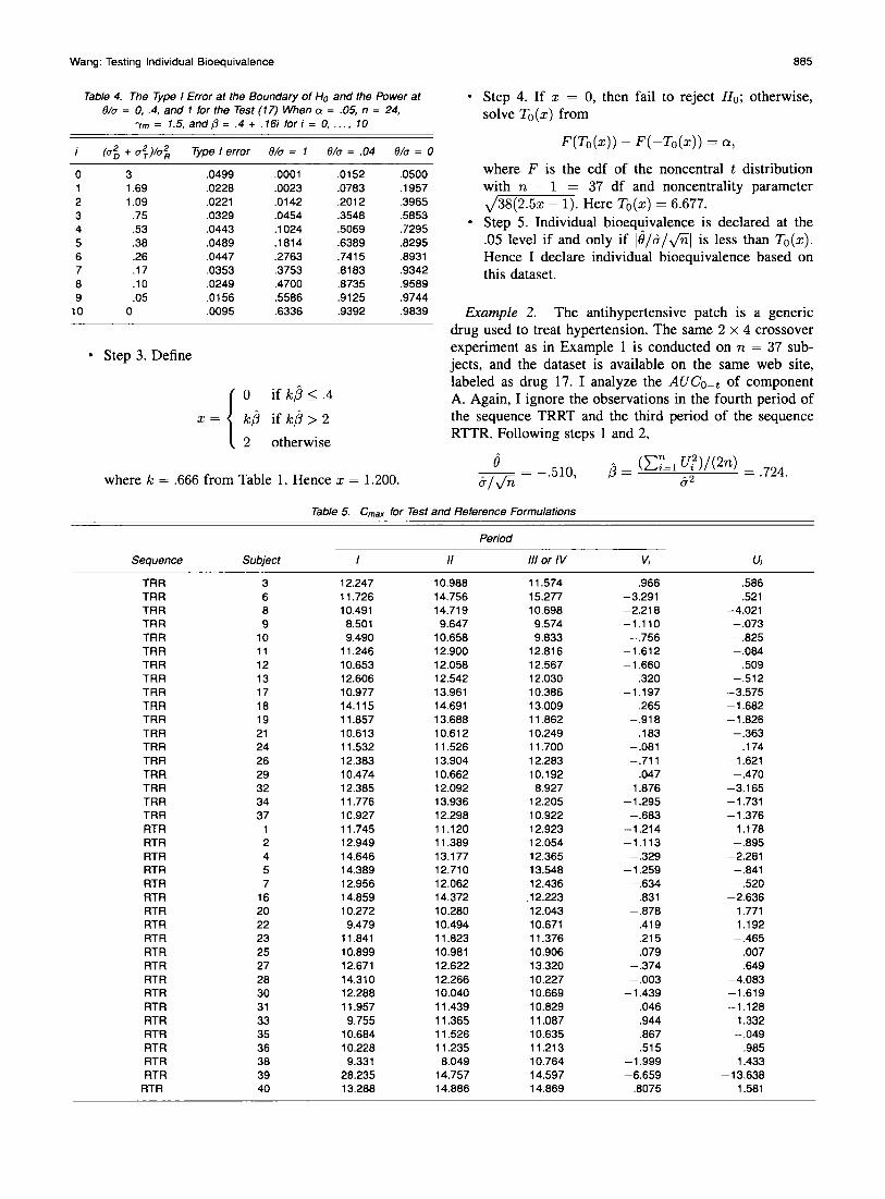
the test and reference formulations are administrated oneach subject once and twice. For the component C of theMAO inhibitor, Cm ax is obtained on two sequences: TRRTand RTTR. Therefore, for the purpose of illustration, I ig­nore the observations in the fourth period of sequence 1and the third period of sequence 2 and pretend to have a2 x 3 crossover design; Table 5 redisplays the data. Notethat subjects 14 and 15 are not given. Thus the sample sizeis n = 38. As pointed out by a referee, in practice moststudies are conducted as four-period designs. For such de­signs, a solution is to use the average of two responsesof test formulation instead of a single response. Somewhatsurprisingly, more parameters and more test statistics areinvolved, and the hypothesis spaces are regions in R3 in­stead of R 2

• This concept is beyond the scope of this article,even though the idea of reparameterization can still be ap­plied, and would be of interest for future research. Assumea three-period design; the analyses on Cm ax proceeds asfollows:

o Step 1. Obtain U, and Vi on each subject using thetransformations (8); for example, V3 = 12.247­(11.574 + 10.988)/2 and U3 = 11.574 - 10.988. Theresults are given in Table 5.

o Step 2. Obtain the sample mean {) = - .607 and thesample standard deviation a = 1.453 of V;'s and thesum of squares of Ui'», L ul = 289.231. Then

{)a/Vii = -2.573,

Table 3. The Type I Error at the Boundary of Ho and the Power atO/a- = 0, .4, and 1 for the Test (14) When 0' = .05, n = 24, "[m = 2,

and (3 = 1/3.5 + (2 - 1/3.5)ilI0 for i = 0, ... , 10

(a-~ + a-~)/a-~ Type I error O/a- = 1 O/a- = .04 O/a- = 0

0 3 .0500 5e-05 .0152 .04991 1.69 .0164 .0023 .1333 .29402 1.09 .0092 .0196 .3525 .58513 .75 .0057 .0731 .5737 .78424 .53 .0040 .1686 .7389 .89335 .38 .0026 .2938 .8467 .94796 .26 .0016 .4266 .9110 .97437 .17 .0010 .5521 .9487 .98708 .10 .0007 .6583 .9701 .99339 .05 .0003 .7440 .9825 .9965

10 0 .0001 .8100 .9896 .9981

Wang: Testing Individual Bioequivalence

Table 4. The Type I Error at the Boundary of Ho and the Power at()/a = 0, .4, and 1 for the Test (17) When Q = .05, n = 24,

"tm = 1.5, and{3 =.4 + .16i fori = 0, ... ,10

(a~ + a~)/a~ Type I error ()ja = 1 ()/a = .04 ()/a = 0

0 3 .0499 .0001 .0152 .05001 1.69 .0228 .0023 .0783 .19572 1.09 .0221 .0142 .2012 .39653 .75 .0329 .0454 .3548 .58534 .53 .0443 .1024 .5069 .72955 .38 .0489 .1814 .6389 .82956 .26 .0447 .2763 .7415 .89317 .17 .0353 .3753 .8183 .93428 .10 .0249 .4700 .8735 .95899 .05 .0156 .5586 .9125 .9744

10 0 .0095 .6336 .9392 .9839

• Step 3. Define

o if k;3 < .4

k;3 if k;3 > 2

2 otherwise

where k = .666 from Table 1. Hence x = 1.200.

885

• Step 4. If x = 0, then fail to reject H o; otherwise,solve To(x) from

F(To(x)) - F( -To(x)) = Q,

where F is the cdf of the noncentral t distributionwith n - 1 = 37 df and noncentrality parameterJ38(2.5x - 1). Here To(x) = 6.677.

• Step 5. Individual bioequivalence is declared at the.05 level if and only if IB/&/Jnl is less than To(x) .Hence I declare individual bioequivalence based onthis dataset.

Example 2. The antihypertensive patch is a genericdrug used to treat hypertension. The same 2 x 4 crossoverexperiment as in Example I is conducted on n = 37 sub­jects, and the dataset is available on the same web site,labeled as drug 17. I analyze the AUCo- t of componentA. Again, I ignore the observations in the fourth period ofthe sequence TRRT and the third period of the sequenceRTTR. Following steps 1 and 2,

o&/In = -.510,

Table 5. Cmax for Test and Reference Formulations

Period

Sequence Subject /I 11/ or IV Vi Vi

TRR 3 12.247 10.988 11.574 .966 .586TRR 6 11.726 14.756 15.277 -3.291 .521TRR 8 10.491 14.719 10.698 -2.218 -4.021TRR 9 8.501 9.647 9.574 -1.110 -.073TRR 10 9.490 10.658 9.833 -.756 -.825TRR 11 11.246 12.900 12.816 -1.612 -.084TRR 12 10.653 12.058 12.567 -1.660 .509TRR 13 12.606 12.542 12.030 .320 -.512TRR 17 10.977 13.961 10.386 -1.197 -3.575TRR 18 14.115 14.691 13.009 .265 -1.682TRR 19 11.857 13.688 11.862 -.918 -1.826TRR 21 10.613 10.612 10.249 .183 -.363TRR 24 11.532 11.526 11.700 -.081 .174TRR 26 12.383 13.904 12.283 -.711 -1.621TRR 29 10.474 10.662 10.192 .047 -.470TRR 32 12.385 12.092 8.927 1.876 -3.165TRR 34 11.776 13.936 12.205 -1.295 -1.731TRR 37 10.927 12.298 10.922 -.683 -1.376RTR 1 11.745 11.120 12.923 -1.214 1.178RTR 2 12.949 11.389 12.054 -1.113 -.895RTR 4 14.646 13.177 12.365 -.329 -2.281RTR 5 14.389 12.710 13.548 -1.259 -.841RTR 7 12.956 12.062 12.436 -.634 -.520RTR 16 14.859 14.372 .12.223 .831 -2.636RTR 20 10.272 10.280 12.043 -.878 1.771RTR 22 9.479 10.494 10.671 .419 1.192RTR 23 11.841 11.823 11.376 .215 -.465RTR 25 10.899 10.981 10.906 .079 .007RTR 27 12.671 12.622 13.320 -.374 .649RTR 28 14.310 12.266 10.227 -.003 -4.083RTR 30 12.288 10.040 10.669 -1.439 -1.619RTR 31 11.957 11.439 10.829 .046 -1.128RTR 33 9.755 11.365 11.087 .944 1.332RTR 35 10.684 11.526 10.635 .867 -.049RTR 36 10.228 11.235 11.213 .515 .985RTR 38 9.331 8.049 10.764 -1.999 1.433RTR 39 28.235 14.757 14.597 -6.659 -13.638

RTR 40 13.288 14.886 14.869 .8075 1.581

886

Now x = k/3 = .479, where k = .662. Solving the equationin step 4, To(.479) = 1.055, and the individual bioequiva­lence is established.

5. OTHER CONSIDERATIONS

The method of constructing the test (14) for (7) can beeasily applied to the following hypotheses:

Ho: I~ I ~ H({3) versus HA : I~ I < H({3), (18)

where H is a given nonnegative nondecreasing function,with the test statistics .;nO/U and /3. Equation (13) can besolved with H m replaced by H, then a new T can be definedas in (14) with an appropriate choice of k.

Return to the hypotheses (6). The parameters a1 and a}are not identifiable based on (8). Therefore, we are not ableto deal with the cases of Cl i- C2. But when Cl = C2 = cand a = 0, then (6) can be written as

where Hg({3) = Vhl + 1.5c){3 - c for {3 E (C/hl +1.5c), 2]. Hence a test can be derived as shown in Section 3.The same test is also a valid test for (6) with a > O. How­ever, this test may be conservative when used for a > O.This is because the null hypothesis of (6) for a > 0 is in­cluded in that for a = O. The hypotheses (6) with a = 0are recommended, because they are invariant under scalechanges and also give higher credits to the test formulationwith a small variability than the hypotheses with a > O.

There is another application for the hypotheses (18).Schall (1995) proposed an individual bioequivalence basedon probability that generalizes (2). He considered the fol­lowing:

Journal of the American Statistical Association, September 1999

where H p is determined by

<I> (rpJ2i] - Hp(;3))VI + ;3/2

_ <I> (_ rpJ2i] + Hp(;3)) = (23)VI + /3/2 Po·

Here <I> is the cdf of N(O, 1) and ;3 E ({3o, 1], where

_ 2[<I>-1(po/2 + 1/2}f{3o - 4r~ - [<I>-1(Po/2 + 1/2)]2'

Moreover, H; is a nondecreasing function.In summary, a method of constructing tests for a general

class of testing problems (18), including individual bioe­quivalence based on moment or probability, has been pro­posed. Higher-order crossover designs (more than 2 x 3)are not necessary for assessing bioequivalence. The simu­lation studies show that the proposed tests are, at least in apractical sense, exact a-level tests. Uniform improvementin power on the proposed tests is possible and of interestfor future research.

APPENDIX: PROOFS

Proof of Lemma 1

Let X~-l = (n - 1)&2Ia 2. For given X~-l,iJ1&1..;n is inde­

pendent of /3, and the conditional distribution of /3 depends on {3only. Therefore, the conditional probability

Pr (I&/~I < T(/3)IX~-l)

=Ej cp(z)dz,{lz+O/u/vnl<Xn_l T(~)/.;n=T}

where cp is the pdf of N(O, 1), is unimodal and symmetric about 0as a function of 01a, as is the unconditional probability

where

H o: PTRI ::; Po versus HA: PTRI > Po, (20)

Proof of Lemma 2

and rp > <I>-1(Po/2 + 1/2)/-./2 and Po are positive con­stants. Here <I> is the cdf of N(O, 1). If the null hypothesisis rejected, then individual bioequivalence is declared. Forexample, if rp = 1.96 and Po = .8, then on more than80% subjects, about 95% of the differences between the re­sponses from the test and reference formulations are within1.96 times -./2aR, the standard deviation of the differencebetween two responses of the reference formulation. Allone needs to do is write (20) in the form of (18).

Lemma 3. The hypotheses (20) can be written as

It is well known that the noncentral t distribution family isstrictly totally positive of order 3 to noncentrality parameter 01a(see Lehmann 1986). Then (12) defines a uniformly most powerfultest for (7) based on the statistic iJ I& by problem 30 of Lehmann(1986, p. 120) for a fixed {3. Because iJI&is maximal invariant withrespect to the group of scale change, (12) defines a uniformly mostpowerful invariant test.

Proof of Lemma 3

Because YiT - YiR follows a normal distribution N(O, (1 +(3/2)u2

) ,

PTRI = <I> (,Py'2fJ - Olu) _ <I> ( IPy'2fJ + OIU) .VI + {3/2 Vi + {3/2

It is clear that PTRI is decreasing in 10lui for any fixed {3. Thus H p

is determined by (5). If the alternative space HA is not empty, then{3 > {3o. To show that H; is nondecreasing, it only must be shown

Wang: Testing Individual Bioequivalence

that PTRI is increasing in fJ. Note that PTRI is an integration ofa standard normal density function on an interval with a radius

IPV2fJ/ JI + fJ/2 and a center at -O/(aJI + fJ/2). The radiusincreases and the center moves toward 0 as fJ gets large. Therefore,for a fixed 0/a, the probability PT RI is increasing in fJ, and theproof is complete.

[Received October 1997. Revised March 1999.J

REFERENCESAnderson, S., and Hauck, W. W. (1983), "A New Procedure for Testing

Equivalence in Comparative Bioavailability and Other Clinical Trials,"Communications in Statistics, Part A-Theory and Methods, 12, 2663­2692.

--- (1990), "Consideration of Individual Bioequivalence,' Journal ofPharmacokinetics and Biopharmaceutics, 18, 259-273.

--- (1996), "Comment," Statistical Science, 11, 303.Brown, L. D., Hwang, J. T. G., and Munk, A. (1997), "An Unbiased Test for

the Bioequivalence Problem," The Annals of Statistics, 26, 2345-2367.Chen, M. L. (1997), "Individual Bioequivalence-A Regulatory Update,"

Journal of Biopharmaceutical Statistics 7, 5--11.Chow, S. C., and Liu, 1. P. (1992), Design and Analysis of Bioavailability

and Bioequivalence Studies, New York: Marcel Dekker.Hwang, J. T. G., and Wang, W. (1997), "The Validity of the Test of Indi­

vidual Equivalence Ratios," Biometrika, 84, 893-900.Lehmann, E. T. (1986), Testing Statistical Hypotheses (2nd ed.), New York:

Wiley.

BB?

Liu, J. P. (1995), "Use of the Repeated Crossover Design in AssessingBioequivalence,' Statistics in Medicine, 14, 1067-1078.

Liu, J. P., and Chow, S. C. (1992), "On Assessment of Bioequivalencein Variability of Bioavailability Studies," Communications in Statistics.Part A-Theory and Methods, 21, 2591-2607.

--- (1996), "Comment," Statistical Science, 11,306-312.Schall, R. (1995), "Assessing of Individual and Population Bioequivalence

Using the Probability that Bioavailabilities are Similar," Biometrics, 51,615---{)26.

Schall, R., and Luus, H. G. (1993), "On Population and Individual Bioe­quivalence,' Statistics in Medicine, 12, 1109-1124.

Schuirmann, D. J. (1987), "A Comparison of the Two One-Sided TestsProcedure and the Power Approach for Assessing the Equivalence ofAverage Bioavailability,' Journal of Pharmacokinetics and Biopharma­ceutics, 15, 657---{)80.

U.S. Food and Drug Administration (1997), Guidancefor 1ndustry:1n VivoBioequivalence Studies Based in Population and Individual Bioequiva­lence Approaches, Rockville, MD: Author.

Wang, W. (1995), "On Assessment of Bioequivalence,' Ph.D. thesis, Cor­nell University.

--- (1997a), "Optimal Unbiased Tests for Equivalence in Intra-SubjectVariability," Journal of the American Statistical Association, 92, 1163­1170.

---(1997b), "Assessing Individual Bioequivalence Using 2 x 2Crossover Design," technical report, Wright State University, Dept. ofMathematics and Statistics.

Wang, W., and Hwang, J. T. G. (1997), "A Nearly Unbiased Test for In­dividual Bioequivalence,' technical report, Cornell University, StatisticsCenter.