On the Abruptness of Bølling–Allerød Warming

ZHAN SU AND ANDREW P. INGERSOLL

Division of Geological and Planetary Sciences, California Institute of Technology, Pasadena, California

FENG HE

Center for Climatic Research, Nelson Institute for Environmental Studies, University of Wisconsin–Madison, Madison,

Wisconsin, and College of Earth, Ocean, and Atmospheric Sciences, Oregon State University, Corvallis, Oregon

(Manuscript received 23 September 2015, in final form 30 March 2016)

ABSTRACT

Previous observations and simulations suggest that an approximate 38–58C warming occurred at intermediate

depths in theNorthAtlantic over severalmillennia duringHeinrich stadial 1 (HS1), which induces warm salty water

(WSW) lying beneath surface cold freshwater. This arrangement eventually generates ocean convective available

potential energy (OCAPE), themaximumpotential energy releasable by adiabatic vertical parcel rearrangements in

an ocean column. The authors find that basin-scale OCAPE starts to appear in the NorthAtlantic (;67.58–73.58N)and builds up over decades at the end ofHS1with amagnitude of about 0.05 J kg21. OCAPEprovides a key kinetic

energy source for thermobaric cabbeling convection (TCC). Using a high-resolution TCC-resolved regional model,

it is found that this decadal-scale accumulation of OCAPE ultimately overshoots its intrinsic threshold and is

released abruptly (;1 month) into kinetic energy of TCC, with further intensification from cabbeling. TCC has

convective plumes with approximately 0.2–1-km horizontal scales and large vertical displacements (;1km), which

make TCC difficult to be resolved or parameterized by current general circulation models. The simulation herein

indicates that these local TCC events are spread quickly throughout the OCAPE-contained basin by internal wave

perturbations. Their convective plumes have large vertical velocities (;8–15 cms21) and bring the WSW to the

surface, causing an approximate 28C sea surface warming for the whole basin (;700 km) within a month. This

exposes a huge heat reservoir to the atmosphere, which helps to explain the abrupt Bølling–Allerød warming.

1. Introduction

In the last deglaciation, the North Atlantic region expe-

rienced notable surface cooling during Heinrich stadial 1

[HS1,;17 ka (1 ka5 1000 years ago); Clark et al. 2002;

Hemming 2004]. Potential surface meltwater discharge

to the North Atlantic, as assumed in numerous studies

(Broecker 1994; Ganopolski and Rahmstorf 2001; Buizert

et al. 2014; Carlson and Clark 2012), may contribute to this

cooling. The cooling is followed by an abrupt (years to de-

cades) surface warming at the end of HS1, that is, at the

onset of the Bølling–Allerød (BA) warming (;14.5ka)

(McManus et al. 2004; Alley 2007). This abrupt warming is

one of the Dansgaard–Oeschger (D–O) warm events (i.e.,

the warming phase of D–O events). As reviewed by

Rahmstorf 2002, there are many mechanisms proposed

to explain the D–O events. (e.g., Liu et al. 2009; Weaver

et al. 2003; Knorr and Lohmann 2007; Ganopolski and

Rahmstorf 2001). With exceptions (e.g., Clement and Cane

1999), most mechanisms are closely related to the Atlantic

meridional overturning circulation (AMOC) such as the

idea of ‘‘thermohaline circulation bistability’’ (Broecker

et al. 1985) and ‘‘salt oscillator’’ (Broecker et al. 1990).

Ganopolski and Rahmstorf (2001, 2002) propose a mech-

anism associated with the stability of AMOCand stochastic

resonance, which explains many key observed features

of D–O events, including the three-phase time evolution,

spatial pattern, and hemispheric seesaw. In this paper, we

focus on themechanism for explaining the abruptness of the

D–O surface warm events (e.g., the abrupt BA warming

during the transition from HS1 to BA). This has not re-

ceived as much attention as the cooling in the North At-

lantic inducedby, for example, the shutdownof theAMOC.

Many previous studies for the D–O warm events in-

volve an established convective-threshold mechanism

Corresponding author address: Zhan Su, Division of Geological

and Planetary Sciences, California Institute of Technology, Pasa-

dena, CA 91125.

E-mail: zssu@caltech.edu

1 JULY 2016 SU ET AL . 4965

DOI: 10.1175/JCLI-D-15-0675.1

� 2016 American Meteorological Society

(e.g., Ganopolski and Rahmstorf 2001; Winton 1995;

Rasmussen and Thomsen 2004; Winton and Sarachik

1993): the cold freshwater (CFW) typically overlies the

warm salty water (WSW) in the North Atlantic after

Heinrich events, where the WSW gradually warms up (as

detailed below). This warming of intermediate-depth

WSW and the potential reduction of surface freshwater

supply reduce the static stability of the ocean until the

threshold of static instability is exceeded in the North At-

lantic. Then the convection renews and brings the WSW

upward. This rapidly releases a large amount of stored

potential energy of heat to the surface and invigorates the

AMOC. Therefore this convective-threshold mechanism

may explain the abrupt D–O warm events. Rahmstorf

(2001) has investigated the threshold onset of convection

(for CFW overlying WSW) and its bistable nature, which

could strongly modulate theAMOC and the climate of the

North Atlantic (see also Rahmstorf 1994, 1995a,b).

In this study we propose amodified convective-threshold

mechanism as an amendment to the above established

convective-threshold mechanism. The main difference is as

follows. In the modifiedmechanism, convection occurs due

to thermobaric instability, which occurs before static in-

stability (the established mechanism) is reached. In other

words, the convection that truly occurs in the BA warming

may be due to the thermobaric instability rather than the

static instability. In contrast to the static instability, ther-

mobaric instability is a different type of fluid instability

(Ingersoll 2005). It not only releases the stored heat of

WSW, but also releases the ocean convective available

potential energy (OCAPE) into kinetic energy of the con-

vection. Further, it typically induces a much more abrupt

(shorter time scale) ocean overturning (verticalmixing) and

typically reaches deeper depths than static instability in

convection events (Denbo and Skyllingstad 1996; Akitomo

1999). Finally, it may provide an intrinsic/self-consistent

component for the climate system. This is because it relies

on the heat/salt transport of the global ocean circulation,

rather than an essentially ‘‘arbitrary’’ surface freshwater

forcing assumed innumerous studies (see section4 formore

discussion). However, whether it substantially changes the

evolution of the BAwarming is less clear. It is possible that

both themodified and the established convective-threshold

mechanisms, if they can both occur, would eventually lead

to a similar final overturning state of the North Atlantic

after years or decades, although what truly occurs may

be the modified mechanism rather than the established

mechanism as mentioned above.

Although the surface freshwater forcing may make

a contribution, both the modified and the established

convective-threshold mechanisms are associated with the

observed millennial-scale (;38–58C) warming at interme-

diate depths (;1–2-km depths) of the North Atlantic

during HS1 (Thiagarajan et al. 2014; Marcott et al. 2011;

Alvarez-Solas et al. 2010). The induced intermediate-depth

ocean is about 48Cwarmer than the shallower water above

[Thiagarajan et al. 2014; see similar observations in

Rasmussen et al. (2003), Rasmussen and Thomsen (2004),

and Dokken and Jansen (1999)]. Many numerical simula-

tions also indicate similar millennial-scale warming (;28–98C) at intermediate depths of North Atlantic, as a re-

sponse to the largely reduced AMOC during stadials

(Shaffer et al. 2004; Stouffer et al. 2006; Clark et al. 2007;

Arzel et al. 2010; Brady and Otto-Bliesner 2011). For ex-

ample, Fig. 1 illustrates the almost 38C warming at around

0.3–2-km depths in theNorthAtlantic duringHS1 (;2300-

yr duration) from the Community Climate System Model,

version 3 (CCSM3), simulation of the last deglaciation (Liu

et al. 2009; He et al. 2013). This phenomenon may have at

least two explanations: 1) Less convective heat is lost into

the atmosphere from the intermediate-depth North At-

lantic due to the suppressed deep convection during sta-

dials (Knutti et al. 2004); also, 2) heat is transported from

the Southern Ocean and tropical Atlantic, which may be

related to the vertical heat diffusion and eddy stirrings, to

the North Atlantic at intermediate depths by the subpolar

gyre and the weakened AMOC during stadials (Winton

1995; Mignot et al. 2007; Shaffer et al. 2004).

In section 2, we demonstrate that millennial-scale

warming at intermediate depths of the North Atlantic

during HS1 could eventually generate OCAPE to a large

FIG. 1. The changes of Atlantic zonal mean potential tempera-

ture u (8C) during HS1 (;2300-yr duration), from the CCSM3

simulation of the last deglaciation (Liu et al. 2009; He et al. 2013).

The figure shows that the North Atlantic became warmer (;1.58–38C) at intermediate depths (beneath;200-m depth) but remained

unchanged or became colder at the ocean surface at 408–808N. This

millennial-scale process generates WSW lying beneath CFW,

which could accumulate OCAPE (Fig. 3).

4966 JOURNAL OF CL IMATE VOLUME 29

magnitude (;0.05 J kg21). OCAPE is a vital kinetic en-

ergy source for thermobaric cabbeling convection [TCC;

see TCC studies inAkitomo et al. (1995), Akitomo (1999,

2006), andHarcourt 2005)]. In section 3, we present high-

resolution numerical simulations for our modified

convective-threshold mechanism: We illustrate that this

continual accumulation of OCAPE eventually overshoots

its intrinsic threshold and causes a sudden release of

OCAPE that powers dramatic TCC events. This brings

warm salty water to the surface and warms the sea sur-

face of the whole basin (;700-km scale) by about 28Cwithin one month. In section 4 we discuss implications.

2. Basin-scale OCAPE in the North Atlantic at theend of HS1

OCAPE is a newly developed and well-defined con-

cept (Su et al. 2016a,b). It quantifies the maximal po-

tential energy of an ocean column that is available to be

released into kinetic energy by the transition from the

current state to the minimum potential energy (PE)

state through adiabatic vertical parcel rearrangements:

OCAPE5PE(current state)2PE(minimum PE state) .

(1)

The same energy concept, although not as formally for-

mulated as OCAPE, was discussed in section 7 of Ingersoll

(2005) and sections 2 and 3 of Adkins et al. (2005). Al-

though OCAPE can be computed numerically for any

idealized equation of state, all OCAPE values in this

manuscript are computed based on the full nonlinear

equation of state of seawater (Jackett et al. 2006). OCAPE

typically appears in an ocean columnwhen cold freshwater

lies above warm salty water. This type of ocean column

may be susceptible to TCC even if the column has a stati-

cally stable stratification. Thus TCC is not the regular sur-

face buoyancy-driven convection. OCAPE offers a main

kinetic energy source for TCC and it arises from thermo-

baricity—the significant increase of the thermal expan-

sion coefficient of seawater with the depth (Fig. 2a). The

appendix illustrates the mechanism for the release of

OCAPE into kinetic energy during TCC events.

TCC is difficult to be directly observed due to its short

time scales (;days) and severe polar observational condi-

tions during wintertime. However, indirect observational

evidences and theoretical or numerical analysis suggest that

the modern Weddell Sea is susceptible to TCC (i.e., the

release of OCAPE to kinetic energy) [detailed in Akitomo

et al. (1995), Akitomo (1999, 2006), McPhee (2000, 2003),

andHarcourt (2005)]. OCAPE exists in themodern ocean:

Figs. 2c,d display a statically stable stratified profile with

CFW overlying WSW that was observed in the Weddell

Sea (McPhee et al. 1996). This profile contains a column-

averaged OCAPE of 1.1 3 1023 Jkg21 [equivalent to a

velocity of 4.7 cms21 if converted into kinetic energy, fol-

lowing the scaling of velocity approximately (2 3 kinetic

energy/mass)0.5]. Figures 2e–h show our simulated TCC

initialized by this observed profile and triggered by realis-

tic surface perturbations (homogeneous brine rejection

equivalent to 1cmday21 sea ice formation, applied to the

whole domain for the initial 4.2 days). The model is two-

dimensional (vertical and horizontal) and nonhydrostatic

in a rotating frame [essentially the samemodel ofAkitomo

et al. (1995) and Akitomo (2006), using the full nonlinear

equation of state from Jackett et al. (2006)]. We apply a

numerical resolution of 50m in the horizontal and 10m in

the vertical, which allows the resolving of TCC (Akitomo

2006; Harcourt 2005). TCC begins after about 2 days and

drives a thorough mixing within 10 days for the whole

10-km domain. The convective plumes have a horizontal

scale of approximately 0.2–1 km and vertical velocities

of 4–7 cms21, which are powered by OCAPE and cabb-

eling effect. This result is consistent with those of Akitomo

(2006), who simulates that TCC causes an approximate

1-km depth of convective overturning for an approxi-

mate 10-km horizontal-scale water column aroundMaud

Rise of theWeddell Sea. TCChence impacts theWeddell

gyre dynamics and the production of Antarctic Bottom

Water there (e.g., Su et al. 2014).

Next we demonstrate that OCAPE could exist in the

North Atlantic at the end of HS1. We use the monthly

output from the CCSM3 simulation of the last deglaciation

(Liu et al. 2009; He et al. 2013. See Fig. 1 for its simulated

intermediate-depth warming during HS1, which induces

CFWoverlyingWSWand thusmay generateOCAPE). As

shown in Figs. 3a–d, we find that a basin-scale OCAPE

pattern first appears in the North Atlantic (;67.58–73.58N)

at about the end of HS1 (14.542ka) and grows larger in

both the horizontal scale (;700 km) and the magnitude

(;0.05Jkg21) for a few decades until the BA warming. In

detail, we show in Fig. 3c a dashed white line (;68W and

67.58–73.58N; 14.536ka) that approximately crosses the

center of the OCAPE pattern. It has CFW (;0–0.5-km

depths) overlying the WSW and has a statically stable

stratification (Fig. 3e). Its averaged OCAPE is about

0.05Jkg21,meaning a convection velocity of approximately

30cms21 if all OCAPE is converted into kinetic energy.

We now discuss the credibility of the build-up of

OCAPE found in CCSM3 (Figs. 3a–d). (i) The OCAPE

of an ocean column is totally determined by its temperature–

salinity (T–S) profile (Su et al. 2016a). Accurate T–S

data for the deglacial climate are scarce. CCSM3 offers

currently one of the most advanced coupled GCM

simulations for the T–S estimate: Through realistic

changes in boundary conditions and forcing, it captures

1 JULY 2016 SU ET AL . 4967

many major features of the deglacial climate evolution,

including some T–S signals as inferred from observa-

tions (Liu et al. 2009; Shakun et al. 2012; Buizert et al.

2014). DiagnosingOCAPE in otherGCMswould be our

future work. (ii) Vertical mixing could partly dissipate

OCAPE (Su et al. 2016b). CCSM3 parameterizes ver-

tical mixing due to breaking internal waves and other

processes (Collins et al. 2006). CCSM3 includes the

mechanism for the diabatic dissipation of OCAPE and

yet OCAPE is present. (iii) As introduced in section 1,

observations indicate about 38–58C warming at in-

termediate depths of the North Atlantic during HS1

(Thiagarajan et al. 2014; Marcott et al. 2011; Alvarez-

Solas et al. 2010). This induces CFW overlying WSW.

Further, the North Atlantic should have a very weak

stratification before the transition from HS1 to BA,

because of either intermediate-depth warming or the

potential surface buoyancy loss (e.g., a decrease of fresh-

water supply at surface) (Ganopolski and Rahmstorf

2001; Rasmussen and Thomsen 2004; Winton 1995).

From Su et al. [2016a, Eqs. (16c) and (17c) therein], for

weakly stratified quasi-two-layer oceans, the OCAPE

is always positive and would increase following the

warming of WSW.1 Therefore, in principle, OCAPE

would be built up due to the intermediate-depth (i.e.,

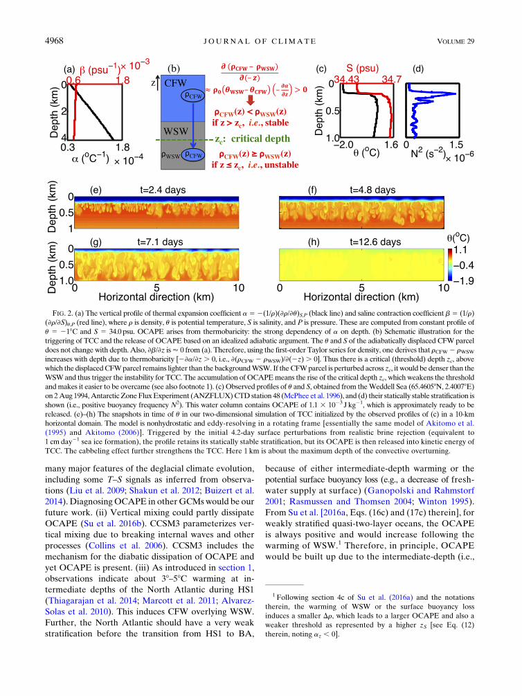
FIG. 2. (a) The vertical profile of thermal expansion coefficient a52(1/r)(›r/›u)S,P (black line) and saline contraction coefficient b5 (1/r)

(›r/›S)u,P (red line), where r is density, u is potential temperature, S is salinity, and P is pressure. These are computed from constant profile of

u 5 218C and S 5 34.0 psu. OCAPE arises from thermobaricity: the strong dependency of a on depth. (b) Schematic illustration for the

triggering of TCC and the release of OCAPE based on an idealized adiabatic argument. The u and S of the adiabatically displaced CFW parcel

does not change with depth. Also, ›b/›z is’ 0 from (a). Therefore, using the first-order Taylor series for density, one derives that rCFW2 rWSW

increases with depth due to thermobaricity [2›a/›z. 0, i.e., ›(rCFW 2 rWSW)/›(2z). 0]. Thus there is a critical (threshold) depth zc, above

which the displacedCFWparcel remains lighter than the backgroundWSW. If theCFWparcel is perturbed across zc, it would be denser than the

WSWand thus trigger the instability for TCC. The accumulation of OCAPEmeans the rise of the critical depth zc, which weakens the threshold

andmakes it easier to be overcame (see also footnote 1). (c) Observed profiles of u and S, obtained from theWeddell Sea (65.46058N, 2.40078E)on 2Aug 1994,AntarcticZoneFluxExperiment (ANZFLUX)CTDstation 48 (McPhee et al. 1996), and (d) their statically stable stratification is

shown (i.e., positive buoyancy frequency N2). This water column contains OCAPE of 1.1 3 1023 J kg21, which is approximately ready to be

released. (e)–(h) The snapshots in time of u in our two-dimensional simulation of TCC initialized by the observed profiles of (c) in a 10-km

horizontal domain. The model is nonhydrostatic and eddy-resolving in a rotating frame [essentially the same model of Akitomo et al.

(1995) and Akitomo (2006)]. Triggered by the initial 4.2-day surface perturbations from realistic brine rejection (equivalent to

1 cm day21 sea ice formation), the profile retains its statically stable stratification, but its OCAPE is then released into kinetic energy of

TCC. The cabbeling effect further strengthens the TCC. Here 1 km is about the maximum depth of the convective overturning.

1 Following section 4c of Su et al. (2016a) and the notations

therein, the warming of WSW or the surface buoyancy loss

induces a smaller Dr, which leads to a larger OCAPE and also a

weaker threshold as represented by a higher zS [see Eq. (12)

therein, noting az , 0].

4968 JOURNAL OF CL IMATE VOLUME 29

WSW) warming before the transition from HS1 to BA.

We emphasize that the intermediate-depth warming

alone (i.e., without surface freshwater forcing) in prin-

ciple can induce the accumulation of OCAPE and the

occurrence of TCC.

OCAPE keeps accumulating to a large magnitude

while the water column remains in a statically stable

stratification. This OCAPE accumulation continuously

weakens the intrinsic threshold (see footnote 1) until

the threshold is finally overshot, after which OCAPE is

then released. Based on an idealized adiabatic argu-

ment, this intrinsic threshold is estimated by the energy

barrier in a stable stratification that CFW parcels have

to overcome to reach the critical depth within the

WSW,where CFWparcels become equally dense as the

surrounding WSW and thermobaricity allows them to

accelerate downward and release OCAPE (Fig. 2b, see

also the appendix). This estimate of threshold, how-

ever, should be treated only conceptually rather than

quantitatively because real-ocean diabatic processes

like cabbeling instability at the CFW–WSW interface

would complicate this estimation (Harcourt 2005).

Although climate models like CCSM3 are capable of

resolving the accumulation of OCAPE as shown above

(Figs. 3a–d), it is difficult for them to account for the

rapid release of OCAPE and thus TCC, for two rea-

sons: 1) Current ocean GCMs have resolutions that are

too coarse to resolve TCC, which has convective

plumes with a typical horizontal scale of approximately

0.2–1 km [e.g., Figs. 2e–h; see alsoAkitomo et al. (1995)

and Akitomo (2006)]. 2) The GCM convective pa-

rameterizations typically apply strong local diapycnal

mixing in the vertical wherever the column is statically

unstable (e.g., the K-profile parameterization; Large

et al. 1994). This cannot account for the effect of TCC:

the acceleration from thermobaricity produces vertical

movement of CFWparcels to large depths (;1 km; e.g.,

Figs. 2f–h) without substantial mixing at intermediate

depths. Therefore, in the CCSM3 simulation the hy-

drographic section shown in Fig. 3e is not followed by

obvious convection (or strong vertical mixing) due to

its statically stable stratification (e.g., Fig. 3e vs Fig. 3f,

showing minimal changes of potential temperature

even after four years). In contrast, we demonstrate in

FIG. 3. (a)–(d) Decadal-scale accumulation of a basin-size (;700 km) OCAPE pattern in the North Atlantic at about the end of HS1,

diagnosed using the monthly output (March data shown here) of the CCSM3 simulation of the last deglaciation (Liu et al. 2009; He et al. 2013).

TheOCAPEpattern starts to appear (a) about 14.542 ka and (b)–(d) grows in size andmagnitude in the following decade. (e)As an example, the

vertical section of u, S, and N2 for the dashed white line displayed in (c) (;68W and 67.58–73.58N; 14.536ka). This section has CFW overlying

WSW,as required forOCAPEgeneration (seeFig. 2b). It has a statically stable stratification (N2. 0) despite of its largeOCAPE.Becauseof this

statically stable stratification, this section is not followed by obvious convection or verticalmixing in theCCSM3 simulation. (f) For example, even

after four years (14.532 ka), the u field still remains roughly unchanged in the CCSM3 simulation. (Contrast this lack of activity with our eddy-

resolving simulation of TCC shown in Fig. 4.) Note that (a)–(d) share the same horizontal and vertical axis, and so do (e) and (f).

1 JULY 2016 SU ET AL . 4969

section 3 that the hydrographic section shown in Fig. 3e

is actually susceptible to TCC using a high-resolution

eddy-resolving simulation (Fig. 4).

3. Simulated abrupt TCC events at the end of HS1

The decadal-scale OCAPE accumulation shown in

Figs. 3a–d may induce TCC at the end of HS1, once the

intrinsic threshold is overshot. Here we use a two-

dimensional high-resolution simulation to investigate

this possibility. The model and its numerical resolution

are the same as the one mentioned in section 2 (for

Figs. 2e–h). We have done simulations at finer resolu-

tions, and they yield consistent results. A 2Dmodel reduces

the computational burden and generates a simulation

of TCC consistent with a 3D model (Akitomo 2006; see

section 4 for more discussion). Our simulation domain

is a depth–latitude section located at around 68W and

67.58–73.58N (white dashed line section shown in Fig. 3c,

;700 km horizontally). The bathymetry of this section is

about 2–2.2 km deep and for convenience we set the

domain bottom at a fixed 2-km depth.

For this section, numerous simulations are tested us-

ing various initializations from decadal-scale monthly

outputs of CCSM3 that contain OCAPE (e.g., the ones

shown in Figs. 3a–d). There are many examples in these

hydrographic snapshots where TCC could occur, among

which the earliest one is most relevant to real-ocean

processes. Here we test various perturbation strengths:

50–200Wm22 homogeneous surface cooling applied for

the whole domain for the initial 1 day,2 which also

generates internal waves. These perturbations represent

the regular strength of wintertime surface buoyancy

forcing in the North Atlantic (Marshall and Schott

1999). We find that all OCAPE patterns earlier than

March at 14.536ka (e.g., Figs. 3a,b) cannot be released

at all into kinetic energy in our test simulations. This is

because for these snapshots, the prescribed perturbations

are not strong enough to cross the threshold of thermo-

baric instability [section 4c of Su et al. (2016a)].However,

with the build-up of OCAPE due to intermediate-

depth warming, the threshold becomes weaker until it

is eventually crossed by the regular strength of per-

turbations. This is the threshold mechanism of why

OCAPE can be accumulated to a large amount and

suddenly triggered to be released into kinetic energy of

TCC (Ingersoll 2005; Adkins et al. 2005).

The earliest snapshot from CCSM3 that is susceptible

to thermobaric instability under our prescribed pertur-

bations is from March at 14.536ka, which initially has a

statically stable stratification (Fig. 3e). Therefore, the

triggered TCC is not based on the established convective-

threshold mechanism, which requires a static instability

(i.e., N2 , 0; see also footnote 2). Here TCC could be

triggered in our simulation by a surface cooling pertur-

bation that is stronger than approximately 70Wm22

(applied for the whole domain for the initial 1 day), which

characterizes the magnitude of threshold for thermobaric

instability for this snapshot of ocean. Further, the trig-

gered TCC and the impact are essentially independent of

the initial trigger as long as the direct contribution of the

perturbation to kinetic energy is small (Su et al. 2016b). In

contrast, the snapshot 1 month earlier (i.e., February at

14.536ka from CCSM3) requires a domain-wide 1-day

surface cooling larger than approximately 800Wm22 for

the triggering of TCC. This contrast of the required per-

turbations (800 vs 70Wm22) is mainly because that from

February toMarch the NorthAtlantic experiences strong

surface buoyancy loss in the GCM, which weakens the

stratification and reduces the threshold for thermobaric

instability (see also footnote 1; again the intermediate-

depthwarming alone could similarly reduce the threshold

to this point, but it would take a longer time). Once

triggered, both snapshots of ocean have been similarly

overturned byTCC for thewhole domainwithin amonth.

Here we focus on the simulation initialized by the snap-

shot of March at 14.536ka, as detailed below.

The associated simulation of TCC is visualized in Fig. 4

(for the whole domain, ;700km wide) and Fig. 5 (for a

local zooming, ;40km wide). After only about 0.6 days

of surface cooling of 100Wm22, the perturbed CFW

plumes sink into the WSW at two separate locations

(;69.88 and 70.88N) nearly simultaneously (Figs. 4b and

5b; see schematic in Fig. 2b). These two locations have

about the maximal initial OCAPE in the whole domain

(Fig. 3c) and are most susceptible to TCC. These initial

convective plumes generate strong internal waves that

spread the initial huge local convective perturbations

(;2km vertically) northward and southward, which are

much stronger perturbations than normal background

internal waves. These trigger other TCC events quickly

along the way for the whole domain (Figs. 4c–e and 5c,d).

These TCC events have convective plumes with hor-

izontal scales of approximately 0.2–1km and large ver-

tical velocities of approximately 8–15 cm s21. They only

occur within the region that initially contains OCAPE,

because TCC is powered by the release of OCAPE into

kinetic energy with further intensification from the

2 This magnitude of cooling changes the ocean stratification by

only a small amount. As a scaling, consider 100Wm22 cooling

applies to the top 100m of water (turbulent mixed layer) for 1 day.

Then this water is cooled by (100Wm22 3 1 day 3 1m2)/

(4200 J kg21 8C21 3 103 kgm23 3 100m3 1m2);0.028C, which is

much smaller than typical sea surface cooling from a big hurricane

system ;18C.

4970 JOURNAL OF CL IMATE VOLUME 29

cabbeling effect. TCC causes strong local (;1-km

depth) turbulent stirring, which vertically mixes the lo-

cal water column within about 8 days (Fig. 5f). For the

entire basin (;700-km scale), these TCC events cause a

thorough vertical mixing (Fig. 4f) and thus increases the

domain-averaged sea surface temperature by around

28C within a month (Fig. 4g). This dramatic surface

warming in North Atlantic exposes a huge basin-scale

heat reservoir to the atmosphere and thus may directly

contribute to the abrupt BA warming. These TCC

events may further contribute to the BA warming by

strengthening the AMOC, which causes more north-

ward heat transport by decadal time scales (e.g.,

Banderas et al. 2012; Hogg et al. 2013; Buizert

et al. 2014).

We also test simulation with the same configuration as

above but excluding thermobaricity in the equation of

state [the equation of state here follows Eq. (17) of Su

et al. (2016b): the vertical profile of thermal expansion

coefficient a(z) should be replaced by a constant a(z 5500m), i.e., the value ofa at the CFW–WSW interface at

;500-m depth in this scenario]. In this scenario the

convection does not occur. This is because our mech-

anism relies on OCAPE to power the convection, while

OCAPE is zero if excluding thermobaricity [see Eqs.

(16c) and (17c) of Su et al. 2016a]. In contrast to

a nonthermobaric convection event (i.e., by static in-

stability), thermobaric instability supports deep pene-

trative convection that alters water properties to typically

greater depths (;2 km), occurs by a more abrupt time

scale (;days), and spreads horizontally in the OCAPE

region.

4. Implications and further work

Our proposed convective threshold is provided by

a quasi-two-layer structure (CFW overlying WSW;

Fig. 4a) and thermobaricity, which permits decadal-scale

FIG. 4. (a)–(f) Snapshots in time of the u field in our eddy-resolving two-dimensional simulation of TCC events in

North Atlantic at about the end of HS1 (;68W and 67.58–73.58N; 14.536 ka). The model is nonhydrostatic and eddy-

resolving in a rotating frame [essentially the samemodel of Akitomo et al. (1995) andAkitomo (2006)], using the full

equation of state of seawater (Jackett et al. 2006). We apply a vertical resolution of 10m and a horizontal resolution

of 50m, which allow the resolving of TCC (Akitomo 2006; Harcourt 2005). The simulation is initialized by the u and S

snapshot output from CCSM3 simulation shown in Fig. 3e. This is the earliest monthly snapshot output that contains

OCAPE (e.g., among Figs. 3a–d and many others) and is also susceptible to TCC in our simulations. Before that, this

region is not susceptible to TCC. The domain size is approximately 700-km horizontal and 2-km vertical, with

a sponge layer on the sides (not shown). TCC is triggered by a 1-day perturbation from inhomogeneous surface

cooling of approximately 100Wm22. Because of the release of OCAPE, TCC starts at about t 5 0.6–0.8 day si-

multaneously at two locations as shown in (b). The convective plumes have a horizontal size of approximately 0.2–

1 km and spread quickly northward and southward by internal wave perturbations as shown in (c)–(f). Within

amonth, this basin-scale NorthAtlantic region (;700 km) has been thoroughlymixed by TCC events as shown in (f),

which increases the sea surface temperature (SST) abruptly by about 28C as shown in (g). [See Fig. 5 for the detail of

convective plumes and its lateral spreading (by zooming into an approximate 40-km horizontal local domain).]

1 JULY 2016 SU ET AL . 4971

accumulation of OCAPE to a large amplitude. This

accumulation process weakens and finally overshoots

the threshold, which releases OCAPE abruptly into ki-

netic energy to minimize the system’s potential energy

(Reddy 2002).

An advantage of our modified convective-threshold

mechanism for the BA warming is that the time scale of

basin-size sea surface warming by TCC events is only

about onemonth, which is much shorter than the years to

hundreds of years’ time scales of regular buoyancy-driven

convection events from the established convective-

threshold mechanism (Ganopolski and Rahmstorf 2001;

see also Buizert et al. 2014; Clark et al. 2002). This is

consistent with previous studies that TCC typically occurs

in a much shorter time scale than regular convection

(Akitomo 1999; Denbo and Skyllingstad 1996). Thus the

time scale of our result is helpful to explain the abrupt

transition from one to three years of observed from the

Greenland during the BA warming (Steffensen et al.

2008).However, the difference between themodified and

the established convective-threshold mechanisms may

not be easily reflected from the paleo observations due to

their relatively low temporal and/or spatial resolutions

(e.g., Thiagarajan et al. 2014). Further, our TCC mecha-

nism is likely tomix the ocean to deeper depths in a single

convection event (Denbo and Skyllingstad 1996), but it is

possible that after years or decades the final overturning

state at the end of the BA warming is the same. Finally,

TCC can be an intrinsic/self-consistent component in the

climate system. This is because TCC relies on the accu-

mulation ofOCAPEby the intermediate-depthwarming,

as a response to the heat/salt transport of the global ocean

circulation. This is in a strong contrast to the simple-

minded configuration of an essentially arbitrary surface

freshwater forcing that controls the convection, which is

used in numerous studies.

As far as we know, our study provides a first simula-

tion to explore the potential importance of thermobaric

instability for the abrupt paleoclimate changes. Our

current simulation is idealized and should be treated

with caveats. (i) Our model does not (and is difficult to)

include the sea ice cover. Martinson (1990) and McPhee

(2003) demonstrate the principal role of sea ice in

maintaining the ocean column’s stability. During con-

vection the warm water brought to the surface would

melt the sea ice and thus restratify the ocean column.

This may offer a strong negative feedback on TCC.

McPhee (2000, 2003) illustrates that thermobaric in-

stability may still overcome this sea ice-induced barrier

in the modern Weddell Sea. Harcourt (2005) simulates

the fact that TCC may fully melt the sea ice cover (see

his Fig. 19c). These studies provide important insights to

explain the Weddell Polynya of the 1970s, which should

be compared to the sea ice melting during the Bølling–Allerød warming. (ii) Sea ice and surface heat fluxes

cool the warm water brought to the surface during

FIG. 5. (a)–(f) As in Figs. 4a–f, but zooming into an approximate 40-km horizontal local domain where TCC first

appears. The convective plumes have a horizontal size of approximately 0.2–1 km. They first appear at t5 0.6 day as

shown in (b) and the consequent perturbations spread laterally and quickly by internal waves. These trigger further

TCC events southward and northward as in (c)–(e). Within 10 days, this approximate 40-km domain has been

thoroughly mixed by TCC events.

4972 JOURNAL OF CL IMATE VOLUME 29

convection, which provides a destabilizing mechanism.

As a test simulation, we restore the SST to the initial

SST with a short relaxation time scale from 10 days to

1month. This effect strengthens the TCC by only a small

amount, since TCC has a short dynamic time scale

(;days; Figs. 4b–d). In general, the ‘‘mixed boundary

condition’’ (e.g., restoring SST and the differential sur-

face salinity flux) is important to modulate the stability

of the thermohaline circulations especially over a time

scale of decades or longer (Yin 1995; Cai 1996;

Mikolajewicz and Maier-Reimer 1994).

More questions need to be investigated in subsequent

studies. (i) Millennial-scale geothermal heating during

HS1, which is not included in this study and in most

climate models, may likely cause significant warming at

ocean depths (Adkins et al. 2005). Thus it may con-

tribute to a larger OCAPE pattern compared to this

study. (ii) Appropriate GCM convection parameteriza-

tions for TCC need to be developed such that TCC ef-

fects can be included in climate models. (iii) TCC is

unlikely to be the only mechanism responsible for the

whole BA warming. It is necessary to investigate the

potential coupling effects between TCC and other im-

portant AMOC-related feedback mechanisms including

ice sheets (e.g., Zhu et al. 2014), sea ice (e.g., the ‘‘sea ice

switch’’ mechanism; see Gildor et al. 2014; Gildor and

Tziperman 2003; Ashkenazy et al. 2013), atmospheric

circulation (e.g., Banderas et al. 2012), the greenhouse

effect (e.g., Zhang et al. 2014), and salt feedback (e.g.,

Knorr and Lohmann 2007). (iv) Our two-dimensional

simulation does not resolve baroclinic instability, which

may trigger TCC (Killworth 1979). It may also occur

shortly after TCC at density fronts formed between the

TCC-induced overturned regions and unoverturned

regions (Akitomo 2006; from a 3D simulation). By

comparing a 3D simulation to a 2D simulation, Akitomo

(2006) finds that baroclinic instability produces additional

upward heat transport (other than that from TCC) and

does not qualitatively change the impacts of TCC. Thus,

including baroclinic instability and using a 3D simulation

may not qualitatively influence our conclusions.

Acknowledgments. We thank Stefan Rahmstorf and

three anonymous reviewers for insightful comments on

the manuscript. We also thank editor Anthony Broccoli

for the constructive suggestions. We thank Jess Adkins

andAndy Thompson for helpful comments on the initial

manuscript. This material is based upon work supported

by the National Science Foundation under Grant AST-

1109299. F.H. was supported by the U.S. NSF (AGS-

1203430) and by the NOAA Climate and Global

Change Postdoctoral Fellowship program, adminis-

tered by the University Corporation for Atmospheric

Research. This research used resources of the Oak Ridge

Leadership Computing Facility at theOakRidgeNational

Laboratory, which is supported by the Office of Science

of the U.S. Department of Energy under Contract

DE-AC05-00OR22725.

APPENDIX

Mechanism for the Release of OCAPE to KineticEnergy

We schematically illustrate the release of OCAPE to

kinetic energy based on idealized assumptions. More

details can be found in Su et al. (2016a,b). Thermobar-

icity is the significant increase of the thermal expansion

coefficient a with the depth 2z. In contrast, the saline

contraction coefficient b is approximately constant with

depth (Fig. 2a). We use the first-order Taylor series of

density with respect to potential temperature u and sa-

linity S [Eq. (29) of Ingersoll 2005]:

r5 r0[12a(u2 u

0)1b(S2 S

0)] , (A1)

where (r0, u0, S0) is the basic state for Taylor expansion.

For two-layer profiles, we consider perturbations (e.g.,

breaking of internal waves or small changes in the buoy-

ancy of the surface ocean) that move CFW parcels down-

ward into WSW (Fig. 2b). The density difference between

the perturbed CFW parcels and the background WSW is

rCFW

2 rWSW

5 r0[2a(u

CFW2 u

WSW)

1b(SCFW

2 SWSW

)] . (A2)

Ideally, if assuming this process is adiabatic, both

uCFW2 uWSW and SCFW2 SWSWwould be constant with

the depth 2z. Noting that b is approximately constant

with depth, we derive from (A2) that rCFW 2 rWSW

would increase with the depth 2z following

›(rCFW

– rWSW

)

›(2z)5 r

0(u

WSW2 u

CFW)

�2›a

›z

�. 0. (A3)

Therefore for a stable stratification, the CFWparcels are

less dense than the WSW (rCFW 2 rWSW , 0) at the

CFW–WSW interface. But if the CFW parcels are per-

turbed downward and eventually cross a certain critical

depth (zc in Fig. 2b), they would become negatively

buoyant (rCFW2 rWSW. 0) due to thermobaricity2›a/

›z from (A3) (Fig. 2b). This releases OCAPE into ki-

netic energy and thus triggers TCC. The above offers a

zero-order picture for the mechanism of TCC. In reality

TCC is strongly modulated by diabatic processes [de-

tailed in Su et al. (2016b)], with further intensification

1 JULY 2016 SU ET AL . 4973

from the cabbeling effect [for cabbeling, see McDougall

(1987)].

REFERENCES

Adkins, J. F., A. P. Ingersoll, and C. Pasquero, 2005: Rapid climate

change and conditional instability of the glacial deep ocean

from the thermobaric effect and geothermal heating. Quat.

Sci. Rev., 24, 581–594, doi:10.1016/j.quascirev.2004.11.005.

Akitomo, K., 1999: Open-ocean deep convection due to thermo-

baricity: 2. Numerical experiments. J. Geophys. Res., 104,

5235–5249, doi:10.1029/1998JC900062.

——, 2006: Thermobaric deep convection, baroclinic instability,

and their roles in vertical heat transport around Maud Rise in

the Weddell Sea. J. Geophys. Res., 111, C09027, doi:10.1029/

2005JC003284.

——, T. Awaji, and N. Imasato, 1995: Open-ocean deep convection

in the Weddell Sea: Two-dimensional numerical experiments

with a nonhydrostatic model. Deep-Sea Res. I, 42, 53–73,

doi:10.1016/0967-0637(94)00035-Q.

Alley, R. B., 2007: Wally was right: Predictive ability of the

North Atlantic ‘‘conveyor belt’’ hypothesis for abrupt cli-

mate change. Annu. Rev. Earth Planet. Sci., 35, 241–272,

doi:10.1146/annurev.earth.35.081006.131524.

Alvarez-Solas, J., S. Charbit, C. Ritz, D. Paillard, G. Ramstein, and

C. Dumas, 2010: Links between ocean temperature and ice-

berg discharge during Heinrich events. Nat. Geosci., 3, 122–

126, doi:10.1038/ngeo752.

Arzel, O., A. Colin de Verdière, andM.H. England, 2010: The role

of oceanic heat transport and wind stress forcing in abrupt

millennial-scale climate transitions. J. Climate, 23, 2233–2256,

doi:10.1175/2009JCLI3227.1.

Ashkenazy, Y., M. Losch, H. Gildor, D. Mirzayof, and

E. Tziperman, 2013: Multiple sea-ice states and abrupt MOC

transitions in a general circulation oceanmodel.Climate Dyn.,

40, 1803–1817, doi:10.1007/s00382-012-1546-2.

Banderas, R., J.Álvarez-Solas, and M. Montoya, 2012: Role ofCO2

and Southern Ocean winds in glacial abrupt climate change.

Climate Past, 8, 1011–1021, doi:10.5194/cp-8-1011-2012.

Brady, E. C., and B. L. Otto-Bliesner, 2011: The role of meltwater-

induced subsurface ocean warming in regulating the Atlantic

meridional overturning in glacial climate simulations. Climate

Dyn., 37, 1517–1532, doi:10.1007/s00382-010-0925-9.

Broecker, W. S., 1994: Massive iceberg discharges as triggers for

global climate change. Nature, 372, 421–424, doi:10.1038/

372421a0.

——,D.M. Peteet, andD.Rind, 1985:Does the ocean–atmosphere

system have more than one stable mode of operation?Nature,

315, 21–26, doi:10.1038/315021a0.

——, G. Bond, M. Klas, G. Bonani, and W. Wolfli, 1990: A salt

oscillator in the glacial Atlantic? 1. The concept. Paleo-

ceanography, 5, 469–477, doi:10.1029/PA005i004p00469.

Buizert, C., and Coauthors, 2014: Greenland temperature response

to climate forcing during the last deglaciation. Science,

345, 1177–1180, doi:10.1126/science.1254961.

Cai, W., 1996: The stability of NADMF under mixed boundary con-

ditions with an improved diagnosed freshwater flux. J. Phys.

Oceanogr., 26, 1081–1087, doi:10.1175/1520-0485(1996)026,1081:

TSONUM.2.0.CO;2.

Carlson, A. E., and P. U. Clark, 2012: Ice sheet sources of sea level

rise and freshwater discharge during the last deglaciation.Rev.

Geophys., 50, RG4007, doi:10.1029/2011RG000371.

Clark, P. U., N.G. Pisias, T. F. Stocker, andA. J.Weaver, 2002: The

role of the thermohaline circulation in abrupt climate change.

Nature, 415, 863–869, doi:10.1038/415863a.

——, S. W. Hostetler, N. G. Pisias, A. Schmittner, and K. J.

Meissner, 2007:Mechanisms for an 7-kyr climate and sea-level

oscillation during marine isotope stage 3. Ocean Circulation:

Mechanisms and Impacts—Past and Future Changes of Me-

ridional Overturning, Geophys. Monogr., Vol. 173, Amer.

Geophys. Union, 209–246, doi:10.1029/173GM15.

Clement, A. C., and M. Cane, 1999: A role for the tropical Pacific

coupled ocean–atmosphere system on Milankovitch and mil-

lennial timescales. Part I: A modeling study of tropical Pacific

variability. Mechanisms of Global Climate Change at Millen-

nial Time Scales, Geophys. Monogr., Vol. 112, Amer. Geo-

phys. Union, 363–372.

Collins, W. D., and Coauthors, 2006: The Community Climate

System Model version 3 (CCSM3). J. Climate, 19, 2122–2143,

doi:10.1175/JCLI3761.1.

Denbo, D. W., and E. D. Skyllingstad, 1996: An ocean large-eddy

simulation model with application to deep convection in the

Greenland Sea. J. Geophys. Res., 101, 1095–1110, doi:10.1029/

95JC02828.

Dokken, T. M., and E. Jansen, 1999: Rapid changes in the mech-

anism of ocean convection during the last glacial period. Na-

ture, 401, 458–461, doi:10.1038/46753.

Ganopolski, A., and S. Rahmstorf, 2001: Rapid changes of glacial

climate simulated in a coupled climate model. Nature, 409,

153–158, doi:10.1038/35051500.

——, and ——, 2002: Abrupt glacial climate changes due to sto-

chastic resonance. Phys. Rev. Lett., 88, 038501, doi:10.1103/

PhysRevLett.88.038501.

Gildor, H., and E. Tziperman, 2003: Sea-ice switches and abrupt

climate change. Philos. Trans. Roy. Soc. London, 361A, 1935–

1944, doi:10.1098/rsta.2003.1244.

——,Y.Ashkenazy, E. Tziperman, and I. Lev, 2014: The role of sea

ice in the temperature–precipitation feedback of glacial cycles.

Climate Dyn., 43, 1001–1010, doi:10.1007/s00382-013-1990-7.

Harcourt, R. R., 2005: Thermobaric cabbeling over Maud Rise:

Theory and large eddy simulation. Prog. Oceanogr., 67, 186–

244, doi:10.1016/j.pocean.2004.12.001.

He, F., J. D. Shakun, P. U. Clark, A. E. Carlson, Z. Liu, B. L. Otto-

Bliesner, and J. E. Kutzbach, 2013: Northern Hemisphere

forcing of Southern Hemisphere climate during the last de-

glaciation. Nature, 494, 81–85, doi:10.1038/nature11822.

Hemming, S. R., 2004: Heinrich events: Massive late Pleisto-

cene detritus layers of the North Atlantic and their global

climate imprint. Rev. Geophys., 42, RG1005, doi:10.1029/

2003RG000128.

Hogg, A. M., H. A. Dijkstra, and J. A. Saenz, 2013: The energetics

of a collapsing meridional overturning circulation. J. Phys.

Oceanogr., 43, 1512–1524, doi:10.1175/JPO-D-12-0212.1.

Ingersoll, A. P., 2005: Boussinesq and anelastic approximations

revisited: Potential energy release during thermobaric in-

stability. J. Phys. Oceanogr., 35, 1359–1369, doi:10.1175/

JPO2756.1.

Jackett, D. R., T. J. McDougall, R. Feistel, D. G. Wright, and S. M.

Griffies, 2006: Algorithms for density, potential temperature,

conservative temperature, and the freezing temperature of sea-

water. J. Atmos. Oceanic Technol., 23, 1709–1728, doi:10.1175/

JTECH1946.1.

Killworth, P. D., 1979: On ‘‘chimney’’ formations in the ocean. J. Phys.

Oceanogr., 9, 531–554, doi:10.1175/1520-0485(1979)009,0531:

OFITO.2.0.CO;2.

4974 JOURNAL OF CL IMATE VOLUME 29

Knorr, G., andG. Lohmann, 2007: Rapid transitions in theAtlantic

thermohaline circulation triggered by global warming and

meltwater during the last deglaciation. Geochem. Geophys.

Geosyst., 8, Q12006, doi:10.1029/2007GC001604.

Knutti, R., J. Flückiger, T. Stocker, and A. Timmermann, 2004:

Strong hemispheric coupling of glacial climate through

freshwater discharge and ocean circulation. Nature, 430, 851–

856, doi:10.1038/nature02786.

Large, W. G., J. C. McWilliams, and S. C. Doney, 1994: Oceanic

vertical mixing: A review and a model with a nonlocal

boundary layer parameterization. Rev. Geophys., 32, 363–403,

doi:10.1029/94RG01872.

Liu, Z., and Coauthors, 2009: Transient simulation of last de-

glaciation with a new mechanism for Bølling–Allerød warm-

ing. Science, 325, 310–314, doi:10.1126/science.1171041.Marcott, S. A., and Coauthors, 2011: Ice-shelf collapse from

subsurface warming as a trigger for Heinrich events. Proc.

Natl. Acad. Sci. USA, 108, 13 415–13 419, doi:10.1073/

pnas.1104772108.

Marshall, J., and F. Schott, 1999: Open-ocean convection: Obser-

vations, theory, and models. Rev. Geophys., 37, 1–64,

doi:10.1029/98RG02739.

Martinson, D. G., 1990: Evolution of the Southern Ocean winter

mixed layer and sea ice: Open ocean deepwater formation and

ventilation. J. Geophys. Res., 95, 11 641–11 654, doi:10.1029/

JC095iC07p11641.

McDougall, T. J., 1987: Thermobaricity, cabbeling, and water-mass

conversion. J. Geophys. Res., 92, 5448–5464, doi:10.1029/

JC092iC05p05448.

McManus, J., R. Francois, J.-M. Gherardi, L. Keigwin, and

S. Brown-Leger, 2004: Collapse and rapid resumption of At-

lantic meridional circulation linked to deglacial climate

changes. Nature, 428, 834–837, doi:10.1038/nature02494.

McPhee,M.G., 2000:Marginal thermobaric stability in the ice-covered

upper ocean over Maud Rise. J. Phys. Oceanogr., 30, 2710–2722,

doi:10.1175/1520-0485(2000)030,2710:MTSITI.2.0.CO;2.

——, 2003: Is thermobaricity a major factor in Southern Ocean

ventilation? Antarct. Sci., 15, 153–160, doi:10.1017/

S0954102003001159.

——, and Coauthors, 1996: The Antarctic Zone Flux Experi-

ment. Bull. Amer. Meteor. Soc., 77, 1221–1232, doi:10.1175/

1520-0477(1996)077,1221:TAZFE.2.0.CO;2.

Mignot, J., A. Ganopolski, and A. Levermann, 2007: Atlantic

subsurface temperatures: Response to a shutdown of the

overturning circulation and consequences for its recovery.

J. Climate, 20, 4884–4898, doi:10.1175/JCLI4280.1.

Mikolajewicz, U., and E. Maier-Reimer, 1994: Mixed boundary

conditions in ocean general circulation models and their in-

fluence on the stability of the model’s conveyor belt.

J. Geophys. Res., 99, 22 633–22 644, doi:10.1029/94JC01989.

Rahmstorf, S., 1994: Rapid climate transitions in a coupled ocean–

atmosphere model. Nature, 372, 82–85, doi:10.1038/372082a0.

——, 1995a: Bifurcations of the Atlantic thermohaline circulation

in response to changes in the hydrological cycle. Nature, 378,

145–149, doi:10.1038/378145a0.

——, 1995b:Multiple convection patterns and thermohaline flow in

an idealized OGCM. J. Climate, 8, 3028–3039, doi:10.1175/

1520-0442(1995)008,3028:MCPATF.2.0.CO;2.

——, 2001: A simple model of seasonal open ocean convection.

Part I: Theory. Ocean Dyn., 52, 26–35, doi:10.1007/

s10236-001-8174-4.

——, 2002: Ocean circulation and climate during the past 120,000

years. Nature, 419, 207–214, doi:10.1038/nature01090.

Rasmussen, T. L., and E. Thomsen, 2004: The role of the North

Atlantic Drift in the millennial timescale glacial climate fluc-

tuations. Palaeogeogr. Palaeoclimatol. Palaeoecol., 210, 101–

116, doi:10.1016/j.palaeo.2004.04.005.

——, D. W. Oppo, E. Thomsen, and S. J. Lehman, 2003: Deep sea

records from the southeast Labrador Sea: Ocean circulation

changes and ice-rafting events during the last 160,000 years.

Paleoceanography, 18, 1018, doi:10.1029/2001PA000736.

Reddy, J. N., 2002: Energy Principles and Variational Methods in

Applied Mechanics. John Wiley & Sons, 592 pp.

Shaffer, G., S. M. Olsen, and C. J. Bjerrum, 2004: Ocean subsurface

warming as a mechanism for coupling Dansgaard–Oeschger

climate cycles and ice-rafting events. Geophys. Res. Lett., 31,L24202, doi:10.1029/2004GL020968.

Shakun, J. D., and Coauthors, 2012: Global warming preceded by

increasing carbon dioxide concentrations during the last de-

glaciation. Nature, 484, 49–54, doi:10.1038/nature10915.Steffensen, J. P., and Coauthors, 2008: High-resolution Greenland

ice core data show abrupt climate change happens in few

years. Science, 321, 680–684, doi:10.1126/science.1157707.

Stouffer, R. J., and Coauthors, 2006: Investigating the causes of the

response of the thermohaline circulation to past and future

climate changes. J. Climate, 19, 1365–1387, doi:10.1175/

JCLI3689.1.

Su, Z., A. L. Stewart, and A. F. Thompson, 2014: An idealized

model of Weddell gyre export variability. J. Phys. Oceanogr.,

44, 1671–1688, doi:10.1175/JPO-D-13-0263.1.

——, A. P. Ingersoll, A. Stewart, and A. Thompson, 2016a: Ocean

convective available potential energy. Part I: Concept and

calculation. J. Phys. Oceanogr., 46, 1081–1096, doi:10.1175/

JPO-D-14-0155.1.

——, ——, ——, and ——, 2016b: Ocean convective available

potential energy. Part II: Energetics of thermobaric convec-

tion and thermobaric cabbeling. J. Phys. Oceanogr., 46, 1097–

1115, doi:10.1175/JPO-D-14-0156.1.

Thiagarajan, N., A. V. Subhas, J. R. Southon, J. M. Eiler, and J. F.

Adkins, 2014: Abrupt pre-Bølling–Allerød warming and cir-

culation changes in the deep ocean. Nature, 511, 75–78,

doi:10.1038/nature13472.

Weaver, A. J., O. A. Saenko, P. U. Clark, and J. X.Mitrovica, 2003:

Meltwater pulse 1A from Antarctica as a trigger of the

Bølling–Allerød warm interval. Science, 299, 1709–1713,

doi:10.1126/science.1081002.

Winton,M., 1995: Energetics of deep-decoupling oscillations. J. Phys.

Oceanogr., 25, 420–427, doi:10.1175/1520-0485(1995)025,0420:

EODDO.2.0.CO;2.

——, and E. Sarachik, 1993: Thermohaline oscillations induced by

strong steady salinity forcing of ocean general circulation

models. J. Phys. Oceanogr., 23, 1389–1410, doi:10.1175/

1520-0485(1993)023,1389:TOIBSS.2.0.CO;2.

Yin, F., 1995: A mechanistic model of ocean interdecadal thermoha-

line oscillations. J. Phys. Oceanogr., 25, 3239–3246, doi:10.1175/

1520-0485(1995)025,3239:AMMOOI.2.0.CO;2.

Zhang, X., G. Lohmann, G. Knorr, and C. Purcell, 2014: Abrupt

glacial climate shifts controlled by ice sheet changes. Nature,

512, 290–294, doi:10.1038/nature13592.

Zhu, J., Z. Liu, X. Zhang, I. Eisenman, andW. Liu, 2014: Linear

weakening of the AMOC in response to receding glacial ice

sheets in CCSM3. Geophys. Res. Lett., 41, 6252–6258,

doi:10.1002/2014GL060891.

1 JULY 2016 SU ET AL . 4975