1

ON THE APPLICATION OF CREDIBILITY THEORY

AND GLMS

JOTHAM NGURI MUCHINA

I56/70122/2011

School of Mathematics

University of Nairobi

A research project submitted in partial fulfillment of the

requirement for the degree of Master of Science in Actuarial Science

of the University of Nairobi.

2

DECLARATION

I declare that ON THE APPLICATION OF CREDIBILITY THEORY AND GLMS is my

own original work. This research project has never been presented for examination at any of the

learning institution/University whether in Kenya or elsewhere as per my own knowledge and

understanding. All the sources quoted have been indicated and acknowledged with complete

reference.

STUDENT

JOTHAM NGURI MUCHINA

SIGN: ------------------------------- DATE: -------------------

This project has been submitted for examination with the approval of the following as University

supervisor.

SUPERVISOR

Prof. P.G.O. Weke

SIGN: ------------------------------- DATE: -------------------

3

ACKNOWLEDGEMENT

I wish to thank in particular my supervisor Prof. P.G.O WEKE, Head, Actuarial Science and

Financial Mathematics Division School of Mathematics for priceless support, understanding and

patience.

4

DEDICATION

This project is dedicated to God and to my family and friends who have supported me all

through the years tirelessly and with dedication.

5

Table of contents

DECLARATION……………………………………………………………………………….....2

ACKNOWLEDGEMENT ………………………………………………………………………..3

DEDICATION………………………………………………………………………………….....4

ABSTRACT……………………………………………………………………………………….7

CHAPTER 1………………………………………………………………………………….......8

1.1: Introduction...............................................................................................................................8

CHAPTER 2……………………………………………………………………………….........11

2.1: Literature Review...................................................................................................................11

CHAPTER 3…………………………………………………………………………………… 13

3.1: Methodology...........................................................................................................................13

3.1.1: The Basic Credibility Theory……………………………………………………………..13

3.1.2: The Credibility Factor..........................................................................................................17

3.2: Limited Fluctuation Method...................................................................................................20

3.2.1: Full Credibility for Frequency.............................................................................................22

3.2.2: Full Credibility for Severity.................................................................................................26

3.3: Greatest Accuracy...................................................................................................................27

3.3.1: Bühlmann Model.................................................................................................................28

6

3.3.2: Bühlmann –Straub...............................................................................................................30

CHAPTER 4.................................................................................................................................32

4.1: Bayesian Credibility...............................................................................................................32

4.1.1: Introduction..........................................................................................................................32

4.1.2: The Poisson/gamma model..................................................................................................33

4.1.3: The normal/normal model...................................................................................................36

4.2: Discussion of the Bayesian approach to credibility................................................................38

CHAPTER 5.................................................................................................................................39

5.1: Generalized Linear Models.....................................................................................................39

5.2: Methodology...........................................................................................................................40

5.2.1: Normal.................................................................................................................................44

5.2.2: Poisson.................................................................................................................................44

5.2.3: Binomial...............................................................................................................................45

5.2.4: Gamma.................................................................................................................................46

5.3: HGLMS and Bühlmann-Straub credibility model.................................................................................48

CHAPTER 6.................................................................................................................................51

CONCLUSIONS AND

RECOMMENDATIONS............................................................................................................51

REFERENCES.............................................................................................................................52

7

ABSTRACT

Premiums are payable to an insurance company for a cover against a certain risk. Credibility

models are actuarial tools to distribute premiums fairly among a heterogeneous group of

policyholders. The problem is usually to devise a way of combining the experience of the group

with the experience of the individual risk the better to calculate the premium. Credibility theory

gives the solution to this problem. Most papers and researches on this subject are difficult to

follow through, especially without the basic knowledge of Credibility theory. They also involve

fairly recondite mathematics. This study describes the basic concept of Credibility theory and the

standard methods of finding the Credibility factor, which are the Limited Fluctuation, Greatest

Accuracy, and Bayesian. This is basically giving the areas of study there are in credibility

theory. Once we have the insurance claim experience with us, we need to fit mathematical

regression models to it. Usually, the data is assumed to be normal, and so we are restricted. The

solution to this problem is the use of Generalized Linear Models which is looked at herein in this

study. The topics at hand are generally broad and therefore for deeper comprehensive study the

reader is advised to look at the numerous original papers on the subject.

8

CHAPTER 1

1.1: INTRODUCTION

Basically, individuals, corporates, businesses and countries are faced by risks every day, e.g.,

risks of fire, or accident. To avoid the downside of such risks, individuals protect themselves by

transferring these risks to an insurance company which agrees to compensate the person or party

for any losses or damages caused by the risks identified in the contract. The insured then is

obliged to pay up some amount known as the premium, or “risk premium". The company, hereby

the insurer, is the one who quotes the amount of premium that is to be paid. There are many

factors that contribute to this amount. The company needs to consider these factors and find

appropriate ways to estimate how much the premium will be. The risks can be grouped together

according to their characteristics, assessed, and then estimation done for the premium. Accuracy

and the degree of accuracy are imperative in this process. Therefore, ways have to be found to

adjust the premium as claim experience is obtained.

The basic idea in insurance is pooling of risks. Individuals who have the “same” exposure to a

particular risk join together to form together a “community-at-risk” in order to bear the perceived

risk. Consider an insurance company with a portfolio consisting of M insured risks numbered i =

1, 2, . . . ,M. In a well-defined insurance period, the risk I produces:

a number of claims Ni,

with claim sizes𝑌𝑖 𝑣 (𝑣 = 1,2,… ,𝑁𝑖),

which together give the aggregate claim amount 𝑋𝑖 = 𝑌𝑖(𝑣)𝑁𝑖

𝑣=1 .

We often refer to the premium payable by the insured to the insurer, for the bearing of the risk,

as the gross premium. The premium volume is the sum, over the whole portfolio, of all gross

premiums in the insurance period. The basic task underlying the rating of a risk is the

determination of the so-called pure risk premium Pi = E [Xi]. Often, we use just the term “risk

9

premium”. The classical point of view assumes that, on the basis of some objectively

quantifiable characteristics, the risks can be classified into homogeneous groups (risk classes),

and that statistical data and theory (in particular, the Law of Large Numbers) then allow one to

determine the risk premium to a high degree of accuracy.

From the dictionary, the word Credibility simply means the quality of being believable or

trustworthy. Credibleness and believability are the other words that can be used in its stead. In

our case we mostly have data or experience to deal with. Therefore we look at whether the said

data or experience is believable or credible such that it can be applied or used. The size in most

cases matters. Basically, the larger the experience or data, the more credible it is said to be. In

many cases a body of data is too small to be fully credible but large enough to have some

credibility. This is where the measurement of credibility comes in where we have a scale from 0

credibility to 1, full credibility.

The word credibility was originally introduced into actuarial science as a measure of the

credence that the actuary believes should be attached to a particular body of experience for rate

making purposes.To say that data is “fully credible” means that the data is sufficient for setting

the premium rates based on it, while the data concerning loss experience is “too small to be

credible” if we believe that the future experience may well be very different, and that we have

more confidence in the knowledge prior to data collection. Many actuarial papers have been

written to discuss credibility. Actuaries use credibility when data is sparse and lacks statistical

reliability.

Credibility theory was first introduced in 1914 by a group of American actuaries. At that time

those actuaries had to define a premium for a new insurance product "workmen's" compensation

- so they based the tariff on a previous kind of insurance which was substituted by this one. As

new experience arrived, a way of including this information was formalized, mixing the new and

the old experiences. This mixture is the basis of credibility theory, which searches for a

credibility estimator that balances the new but volatile data, and the old but with a historical

support. Most of the research until 1967 went in this direction, creating the branch of credibility

theory called limited fluctuation. The turning point in this theory, and the reason why it is used

nowadays, happened when actuaries realized that they could bring such a mixture idea inside a

portfolio. This new branch searches for an individual estimator (or a class estimator), but still

10

using the experience for the whole portfolio. Such an estimator would consider the "own"

experience on one side, but giving more confidence to it by also including a more "general" one

on the other side. In a way, it formalizes the mutuality behind insurance, without the loss of the

individual experience. There are many papers discussing this theory, but the one by Bühlmann

(1967) is generally seen as a landmark. In this paper credibility theory was completely

formalized, giving a basic formula and philosophy. Since then, many models have been

developed.

In the recent past, credibility theory has become a cornerstone and of great importance in

Actuarial Science. It is very important as it helps to calculate premiums for a group of insurance

contracts.Credibility theory has its core in Bayesian statistics.

We later on introduce the Generalized Linear Models. In the process of regressing insurance

claims data, we are usually restricted to normal data only. The problem arises when the data

proves different from normal. This is where GLMs come in. they allow us to no longer be

restricted but now to have regression extended to distributions form the exponential family.

The framework of HierarchicalGeneralized Linear Models allows a more extensive range of

models to be used thanstraightforward credibility theory. Thus, this study contributes a

furtherrange of models which may be useful in a wide range of actuarial applications,

includingpremium rating.

The aim of this study is to simplify as much as possible the topic of Credibility Theory and give

a rather more straightforward approach to it, not forgetting to describes the basic concept of

Credibility theory and the standard methods of finding the Credibility factor, which are the

Limited Fluctuation, Greatest Accuracy, and Bayesian. Also, to introduce GLMs and connect to

Credibility Theory.Chapter two gives the literature review of the study. Chapter three explains

the basic credibility theory and the credibility factor. It also explains the standard methods of

finding the credibility factor, which include the Limited Fluctuation method and the Greatest

Accuracy method. It is usual to have the assumption that credibility theory is completely based

on Bayesian statistics. This is what chapter four is about. Bayesian credibility is the third method

of finding the credibility factor. Chapter five explains the Generalized Linear Models.

11

CHAPTER 2

2.1: LITERATURE REVIEW

The study and writing of papers about Credibility theory began with the papers by Mowbray

(1914) and Whitney (1918), whereby the emphasis was on deriving a premium which was a

balance between the experience of an individual risk and of a class of risks. Bühlmann (1967)

showed how a credibility formula can be derived in a distribution-free way, using a least squares

criterion. Since then, a number of papers have shown how this approach can be extended. See

particularly Bühlmann and Straub (1970), Hachemeister (1975), de Vylder (1976, 1986). The

survey by Goovaerts and Hoogstad (1987) provides an excellent introduction to these papers.

The underlying assumption of credibility theory which sets it apart from formulae based on the

individual risk alone is that the risk parameter is regarded as a random variable. This naturally

leads to a Bayesian model, and there have been a large number of papers which adopt the

Bayesian approach to credibility theory: for example Jewell (1974, 1975), Klugman (1987),

Zehnwirth (1977) Klugman (1992) gives an introduction to the use of Bayesian methods,

covering particularly aspects of credibility theory. A recent review of Bayesian methods in

actuarial science and credibility theory is given by Makov et al (1996)

Developed in the early part of the 20th century, limited fluctuations credibility gives formulas

to assign full or partial credibility to a policyholder's, or group of policyholders' experience.

Bühlmann (1967, 1969), Bühlmann and Straub (1970), Hachemeister (1975), Jewell (1975) and

Frees (2003) give several credibility formulas. Goulet et al. (2006) gives a review of four

different formulas.

McCullagh and Nelder (1989) provide a detailed introduction to GLMs and also offer actuarial

illustrations in their study. The books by Aitkin et al. (1989) and Dobson (1990) are also

12

excellent references with many examples of applications of GLMs. Haberman and Renshaw

(1996) give a comprehensive review of the applications of GLMs to actuarial problems.

McCulloch and Searle (2001) and Demindenko (2004) are useful references for details on

GLMMs. Antonio and Beirlant (2006) give an application of GLMMs in actuarial statistics.

Nelder and Verrall (1997) shows how credibility theory can be encompassed within the theory of

GLMs. They set the relationship between credibility theory and generalized linear models by

using Bühlmann model among credibility models and hierarchical generalized linear model in

likelihood basis among statistical models.

13

CHAPTER 3

3.1: METHODOLOGY

3.1.1: THE BASIC CREDIBILITY THEORY

Simply put, credibility theory is a technique that can be used to determine premiums or claim

frequencies in general insurance. The word credibility was originally introduced into actuarial

science as a measure of the acceptance that the actuary believes should be attached to a particular

body of experience for rate making purposes.

The beginnings of credibility dates back to Whitney, who in 1918 addressed the problem of

assessing the risk premium C, defined as the expected claims expenses per unit of risk exposed,

for an individual risk selected from a portfolio (class) of similar risks. Recommending the

combined use of individual risk experience and class risk experience, he proposed that the

premium rate be a weighted average of the form

𝐶 = 𝑧𝑋 + (1 − 𝑧)𝐶

Where X is the observed mean claim amount per unit of risk exposed for the individual contract

and is the corresponding overall mean in the insurance portfolio. Whitney viewed the risk

premium as a random variable.

Credibility is a technique for pricing insurance coverages that is widely used by health, group

term life, and property and casualty actuaries.

Generally, Credibility theory provides tools to deal with the randomness of data that is used for

predicting future events or costs. For example, an insurance company uses past loss information

of an insured or group of insureds to estimate the cost to provide future insurance coverage. But,

insurance losses arise from random occurrences. The average annual cost of paying insurance

losses in the past few years may be a poor estimate of next year's costs. The expected accuracy of

14

this estimate is a function of the variability in the losses. This data by itself may not be

acceptable for calculating insurance rates.

Rather than relying solely on recent observations, better estimates may be obtained by

combining this data with other information. For example, suppose that recent experience

indicates that Juakali Inc. should be charged a rate of Kshs.500 (per Kshs.10000 of payroll) for

workers compensation insurance. Assume that the current rate is Ksh.1000. What should the new

rate be? Should it be Kshs.500, Kshs.1000, or somewhere in between? Credibility is used to

weight together these two estimates.

The basic formula 𝐶 = 𝑧𝑋 + (1− 𝑧)𝐶 for calculating credibility weighted estimates that we

got earlier can be written as:

Estimate = Z× [Observation] +(1-Z)× [Other Information],

0≤Z≤1

where Z is the credibility assigned to the observation. 1-Z is generally referred to as the

complement of credibility. If the body of observed data is large and not likely to vary much from

one period to another, then Z will be closer to one. On the other hand, if the observation consists

of limited data, then Z will be closer to zero and more weight will be given to other information.

The current rate of Ksh.1000 in the above example is the "Other Information." It represents an

estimate or prior hypothesis of a rate to charge in the absence of the recent experience. As recent

experience becomes available, then an updated estimate combining the recent experience and the

prior hypothesis can be calculated. Thus, the use of credibility involves a linear estimate of the

true expectation derived as a result of a compromise between observation and prior hypothesis.

The JuakaliInc's rate for workers compensation insurance is

Z×Ksh.500+(1-Z)×Kshs.1000 under this model.

The general goal of credibility as used in Actuarial science is to improve statistical estimates,

for example the premium estimates. The actuary uses observations of events that happened in the

past to forecast future events or costs. For example, data that was collected over several years

about the average cost to insure a selected risk, sometimes referred to as a policyholder or

15

insured, may be used to estimate the expected cost to insure the same risk in future years.

Because insured losses arise from random occurrences, however, the actual costs of paying

insurance losses in past years may be a poor estimator of future costs.

Consider a risk that is a member of a particular class of risks. Classes are groupings of risks

with similar risk characteristics, and though similar, each risk is still unique and not quite the

same as other risks in the class. In class rating, the insurance premium charged to each risk in a

class is derived from a rate common to the class. Class rating is often supplemented with

experience rating so that the insurance premium for an individual risk is based on both the class

rate and actual past loss experience for the risk. The important question in this case is: How

much should the class rate be modified by experience rating? That is, how much credibility

should be given to the actual experience of the individual risk? Two factors are important in

finding the right balance between class rating and individual rating. These are the two ways: one

is when the portfolio is homogeneous, and the other when the portfolio is heterogeneous. When

the portfolio given is homogeneous, then all of the risks in the class are identical and have the

same expected value for losses. Here we therefore can charge the same premium to everyone in

that particular portfolio. This is estimated by the overall mean X of the data. On the other hand,

if the portfolio is not homogeneous, this method can be problematic as `'good" risk people will

be overcharged and those considered as `'bad" risk people will be undercharged. Consequently,

the `'good" risks will take their business elsewhere, leaving the insurer with only `'bad" risks.

This is actually what is known as adverse selection. If the portfolio is heterogeneous, and the

claim experience is fairly large, we can charge to each group j its own average claims, being X as

premium charged to the insured. To compromise these two extreme positions, we take the

weighted average of these two extremes:

C=zjXj+(1-zj)Xj

If the group were completely homogeneous then it would be reasonable to set zj=0, while if

the group were completely heterogeneous then it would be reasonable to set zj=1. Using

intermediate values is reasonable to the extent that both individual and group history are useful

in inferring future individual behavior.

16

The following is a very simple example:

Suppose a bus company in Nairobi has run a fleet of ten buses for a number of years. The bus

company wishes to insure this fleet for the coming year against claims arising from accidents

involving these buses. The pure premium for this insurance needs to be calculated, i.e. the

expected cost of claims in the coming year. The data for the past five years for this particular

fleet of buses show that the average cost of claims per annum (for the ten buses) has been Ksh.

224,000. Suppose that, in addition to this information, there is data relating to a large number of

bus companies fleets from all over the country which show that the average cost of claims per

annum per bus is Ksh. 35,000, so that the average cost of claims per annum for a fleet of ten

buses is Ksh. 350,000. However, while this figure of Ksh. 350,000 is based on many more fleets

of buses than the figure of Ksh. 224,000, some of the fleets of buses included in this large data

set operate under very different conditions (which are thought to affect the number and/or size of

claims, e.g. in large cities or in rural areas) from the particular fleet which is of concern here.

There are two extreme choices for the pure premium for the coming year:

1. Ksh. 224,000 could be chosen on the grounds that this estimate is based on the most

appropriate data, whereas the estimate of Ksh. 350,000 is based on less relevant data, or,

2. Ksh. 350,000 could be chosen on the grounds that this is based on more data and so is, in

some sense, a more reliable figure.

The credibility approach to this problem is to take a weighted average of these two extreme

answers, i.e. to calculate the pure premium as:

Z × 224,000 + (1 - Z) × 350,000

where Z is the credibility factor. We now need to find out the value of Z.

The following is another example also demonstrating how credibility can help produce better

estimates:

In a large population of automobile drivers, the average driver has one accident every five

years or, equivalently, an annual frequency of 0.20 accidents per year. A driver selected

randomly from the population had three accidents during the last five years for a frequency of

17

0.60 accidents per year. What is your estimate of the expected future frequency rate for this

driver? Is it 0.20, 0.60, or something in between?

Solution: If we had no information about the driver other than that he came from the

population, we should go with the 0.20. However, we know that the driver's observed frequency

was 0.60. Should this be our estimate for his future accident frequency?Probably not. There is a

correlation between prior accident frequency and future accident frequency, but they are not

perfectly correlated. Accidents occur randomly and even good drivers with low expected

accident frequencies will have accidents. On the other hand, bad drivers can go several years

without an accident. A better answer than either 0.20 or 0.60 is most likely something in

between: this driver's Expected Future Accident Frequency = Z x 0.60+(1 x Z) x 0.20

The key to finishing the solution for this example is the calculation of Z. How much

credibility should be assigned to the information known about the driver?

Before we look at the solution to this, let us note a few things about the credibility factor.

3.1.2: THE CREDIBILITY FACTOR

Z is a number between 0 and 1 and is called the credibility weight or credibility factor. It

expresses how credible or acceptable an item or estimate is. In credibility of data, 0 credibility is

given to data that is too small to be used for premium rate making. If some data has credibility of

1, this means the data is fully credible.

Its value reflects how much "trust" is placed in the data from the risk itself (X) compared with

the data from the larger group (µ). As an estimate of next year's expected aggregate claims or

number of claims, the higher the value of Z, the more trust is placed in X compared with μ and

vice versa. It can be seen that, in general terms, the credibility factor would be expected to

behave as follows:

-- The more data there are from the risk itself, the higher should be the value of the credibility

factor.

18

-- The more relevant the collateral data, the lower should be the value of the credibility factor.

While the value of the credibility factor should reflect the amount of data available from the

risk itself, its value should not depend on the actual data from the risk itself.

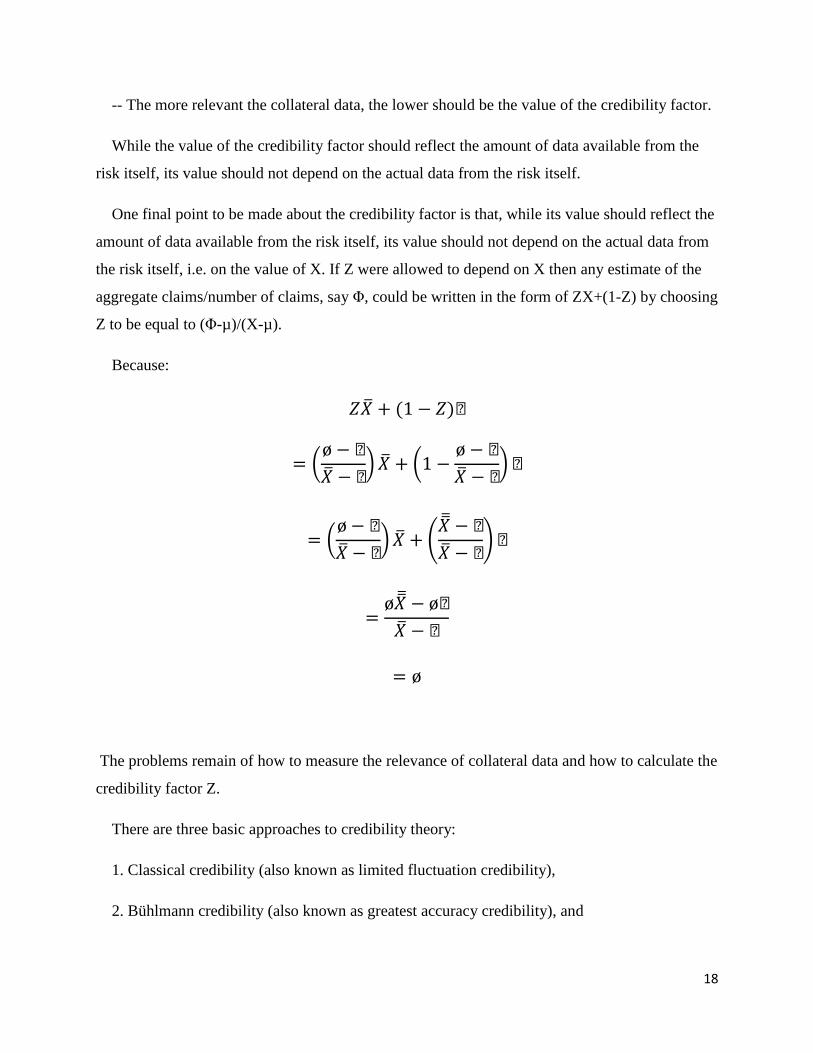
One final point to be made about the credibility factor is that, while its value should reflect the

amount of data available from the risk itself, its value should not depend on the actual data from

the risk itself, i.e. on the value of X. If Z were allowed to depend on X then any estimate of the

aggregate claims/number of claims, say Φ, could be written in the form of ZX+(1-Z) by choosing

Z to be equal to (Φ-µ)/(X-µ).

Because:

𝑍𝑋 + (1− 𝑍)µ

= ø− µ

𝑋 − µ 𝑋 + 1−

ø− µ

𝑋 − µ µ

= ø− µ

𝑋 − µ 𝑋 +

𝑋 − µ

𝑋 − µ µ

=ø𝑋 − øµ

𝑋 − µ

= ø

The problems remain of how to measure the relevance of collateral data and how to calculate the

credibility factor Z.

There are three basic approaches to credibility theory:

1. Classical credibility (also known as limited fluctuation credibility),

2. Bühlmann credibility (also known as greatest accuracy credibility), and

19

3. Bayesian credibility.

Bayesian credibility is the most accurate way to determine a credibility-weighted mortality

assumption. But it's impractical to apply in practice because the distribution assumptions needed

aren't straightforward and require a lot of judgment. It also can create occasional biases because

subjectivity is required in the assumptions.

Bühlmann credibility is more theoretically sound. But used in the traditional way, Bühlmann

credibility is less practical to apply to mortality studies because mortality needs to be estimated

for a given risk class, not for exposure with an unknown risk class. It's also often difficult to get

enough experience for this method to be useful.

Classical credibility is much easier to use compared to the other methods because it uses a

simple formula and gives reasonable results in almost all scenarios. It also handles the problem

of having limited experience because it uses underlying assumptions to judge credibility and

doesn't rely heavily on the experience. The only criterion that classical credibility may not satisfy

is that it may not give unbiased results because some judgment is required to apply the method.

In most cases, classical credibility can be a good guide to assess the credibility of past

mortality experience. In the case where a more accurate estimate of credibility may be warranted,

Bayesian credibility should be applied because it's the most accurate technique. Regardless of

which method is used, it should follow the four basic guidelines to be sound:

- Produce reasonable results;

- Be practical in its application;

- Provide results that are not materially biased;

- Balance the responsiveness of mortality expectation to experience while minimizing

fluctuations in mortality expectations

20

3.2: LIMITED FLUCTUATION METHOD

The Limited Fluctuation method uses only the policy by policy experience study results of a

single company. Consequently, each company can calculate their own estimate using the Limited

Fluctuation method. It is referred to as limited fluctuation credibility because it attempts to limit

the effect that random fluctuations in the observations will have on the estimates. The credibility

Z is a function of the expected variance of the observations versus the selected variance to be

allowed in the first term of the credibility formula, Z × [Observation].

It provides a criterion for full credibility based on the size of the portfolio. Full credibility

means it is appropriate to use only the portfolio's own experience and to ignore the entire

industry data. In addition, it provides an ad hoc methodology for the determination of partial

credibility, where there is a weighting of the portfolio's own experience and the industry

experience.

The genealogy of the limited fluctuations approach takes us back to 1914, when Mowbray

suggested how to determine the amount of individual risk exposure needed for X to a fully

reliable estimate of X. He worked with annual claim amounts X₁,...,Xn, assumed to be i.i.d.

(independent and identically distributed) selections from a probability distribution with density

f(x|θ), mean m(θ), and variance s²(θ). The parameter θ was viewed as non-random.

Specifically, it was in the workers’ compensation insurance field where Mowbray was

interested in finding the minimal number of employees covered by a plan such that the premium

of the employer could be considered fully dependable, that is, fully credible. Assuming that the

probability of an accident, , is known, Mowbray wanted to calculate the minimum number of

employees, n, so that the number of accidents would lie within 100k percent of the average (or

mode) with probability p. if N denotes the total number of accidents of an employer, Mowbray's

problem can be written as:

P[(1-k)E[N]≤N≤(1+k)E[N]]≥p,

Where N~binomial (n,θ), i.e., N is binomial with mean n and variance nθ(1-θ). Using the

normal approximation for N eliminates the choice between the mean and the mode and yields:

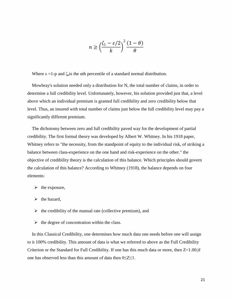
21

𝑛 ≥ 𝜁1 − 𝜀/2

𝑘

2 1− 𝜃

𝜃

Where ε =1-p and ζαis the αth percentile of a standard normal distribution.

Mowbray's solution needed only a distribution for N, the total number of claims, in order to

determine a full credibility level. Unfortunately, however, his solution provided just that, a level

above which an individual premium is granted full credibility and zero credibility below that

level. Thus, an insured with total number of claims just below the full credibility level may pay a

significantly different premium.

The dichotomy between zero and full credibility paved way for the development of partial

credibility. The first formal theory was developed by Albert W. Whitney. In his 1918 paper,

Whitney refers to "the necessity, from the standpoint of equity to the individual risk, of striking a

balance between class-experience on the one hand and risk-experience on the other." the

objective of credibility theory is the calculation of this balance. Which principles should govern

the calculation of this balance? According to Whitney (1918), the balance depends on four

elements:

the exposure,

the hazard,

the credibility of the manual rate (collective premium), and

the degree of concentration within the class.

In this Classical Credibility, one determines how much data one needs before one will assign

to it 100% credibility. This amount of data is what we referred to above as the Full Credibility

Criterion or the Standard for Full Credibility. If one has this much data or more, then Z=1.00;if

one has observed less than this amount of data then 0≤Z≤1.

22

Exactly how to determine the amount of credibility assigned to different amounts of data is

discussed in the following sections.

There are four basic concepts from Classical Credibility which will be covered:

1. How to determine the criterion for Full Credibility when estimating frequencies;

2. How to determine the criterion for Full Credibility when estimating severities;

3. How to determine the criterion for Full Credibility when estimating pure premiums (loss

costs);

4. How to determine the amount of partial credibility to assign when one has less data than is

needed for full credibility.

Below we look at the first two with interest in estimating frequencies and severities.

3.2.1: FULL CREDIBILITY FOR FREQUENCY

Assume we have a Poisson process for claim frequency, with an average of 500 claims per

year. Then, the observed numbers of claims will vary from year to year around the mean of 500.

The variance of a Poisson process is equal to its mean, in this case 500. This Poisson process can

be approximated by a Normal Distribution with a mean of 500 and a variance of 500.

The Normal Approximation can be used to estimate how often the observed results will be far

from the mean. For example, how often can one expect to observe more than 550 claims? The

standard deviation is √(500)=22.36. So 550 claims corresponds to about 50/22.36 = 2.24

standard deviations greater than average. Since Φ(2.24)=0.9875, there is approximately a 1.25%

chance of observing more than 550 claims.

Thus there is about a 1.25% chance that the observed number of claims will exceed the

expected number of claims by 10% or more. Similarly, the chance of observing fewer than 450

claims is approximately 1.25%. So the chance of observing a number of claims that is outside the

range from -10% below to +10% above the mean number of claims is about 2.5%. In other

23

words, the chance of observing within ±10% of the expected number of claims is 97.5% in this

case.

More generally, one can write this algebraically. The probability P that observation X is within

±k of the mean µ is:

P =Prob[µ-µk≤X≤µ+kµ]

=Prob [-k (µ/σ)≤(X-µ)/σ ≤ k (µ/σ)]

The last expression is derived by subtracting through by µ and then dividing through by

standard deviation σ. Assuming the Normal Approximation, the quantity u=(X-µ)/σ is normally

distributed. For a Poisson distribution with expected number of claims n, then µ=n and σ=√n.

The probability that the observed number of claims N is within ±k% of the expected number µ=n

is:

P=Prob[-k√n≤µ≤k√n]

In terms of the cumulative distribution for the unit normal, Φ(u):

P= Φ (k√n)- Φ (-k√n)= Φ (k√n)-(1- Φ (k√n))

=2 Φ (k√n)-1

Thus, for the Normal Approximation to the Poisson:

P=2 Φ (k√n)-1

Or, equivalently:

Φ (k√n)=(1+P)/2

To use an example for illustration:

If the number of claims has a Poisson distribution, compute the probability of being within

±5% of a mean of 100 claims using the Normal Approximation to the Poisson.

The solution should be: 2 Φ (0.05√(100))-1=38.29%

24

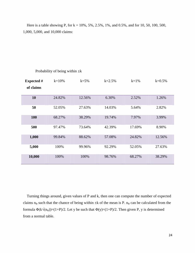
Here is a table showing P, for k = 10%, 5%, 2.5%, 1%, and 0.5%, and for 10, 50, 100, 500,

1,000, 5,000, and 10,000 claims:

Probability of being within ±k

Expected #

of claims

k=10% k=5% k=2.5% k=1% k=0.5%

10 24.82% 12.56% 6.30% 2.52% 1.26%

50 52.05% 27.63% 14.03% 5.64% 2.82%

100 68.27% 38.29% 19.74% 7.97% 3.99%

500 97.47% 73.64% 42.39% 17.69% 8.90%

1,000 99.84% 88.62% 57.08% 24.82% 12.56%

5,000 100% 99.96% 92.29% 52.05% 27.63%

10,000 100% 100% 98.76% 68.27% 38.29%

Turning things around, given values of P and k, then one can compute the number of expected

claims n₀ such that the chance of being within ±k of the mean is P. n₀ can be calculated from the

formula Φ(k√(n₀))=(1+P)/2. Let y be such that Φ(y)=(1+P)/2. Then given P, y is determined

from a normal table.

25

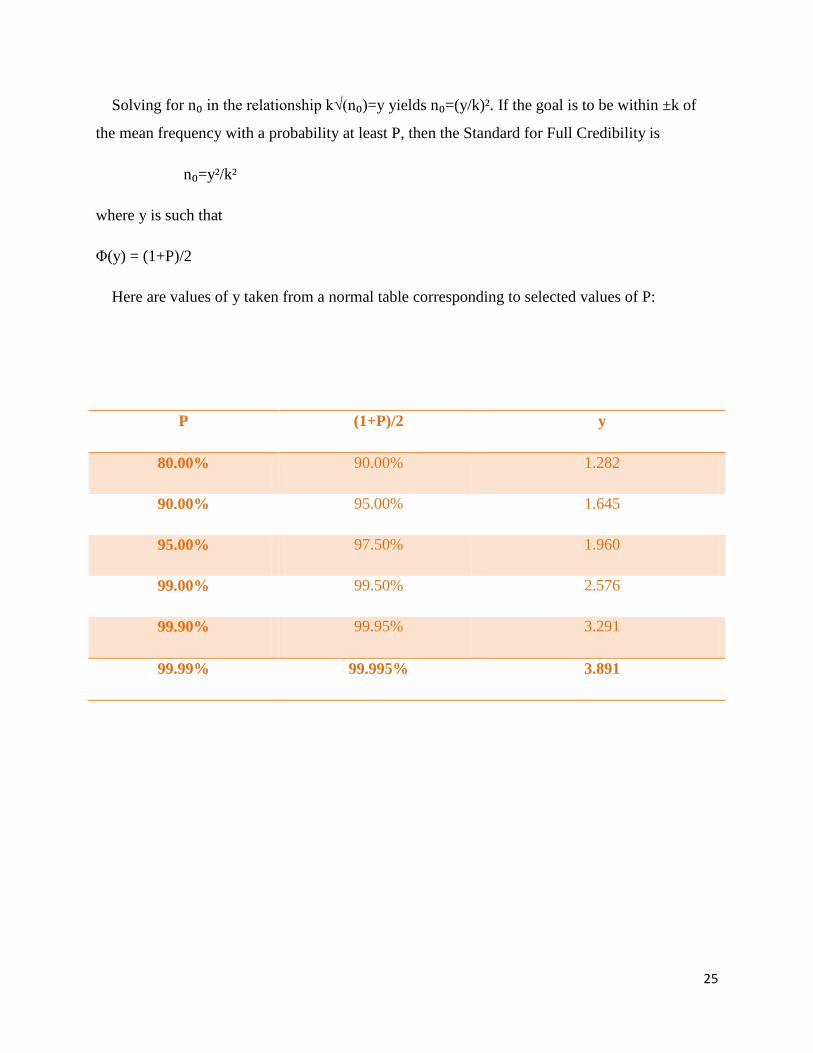
Solving for n₀ in the relationship k√(n₀)=y yields n₀=(y/k)². If the goal is to be within ±k of

the mean frequency with a probability at least P, then the Standard for Full Credibility is

n₀=y²/k²

where y is such that

Φ(y) = (1+P)/2

Here are values of y taken from a normal table corresponding to selected values of P:

P (1+P)/2 y

80.00% 90.00% 1.282

90.00% 95.00% 1.645

95.00% 97.50% 1.960

99.00% 99.50% 2.576

99.90% 99.95% 3.291

99.99% 99.995% 3.891

26

3.2.2: FULL CREDIBILITY FOR SEVERITY

The Classical Credibility ideas also can be applied to estimating claim severity, the average

size of a claim.

Suppose a sample of N claims, X₁,X₂,...XN, are each independently drawn from a loss

distribution with mean µs and variance σs².

The severity, i.e. the mean of the distribution, can be estimated by (X₁+X₂+...+ XN)/N. The

variance of the observed severity is Var (∑Xi/N)=(1/N²)∑ Var(Xi)= σs²/N. Therefore, the

standard deviation for the observed severity is σs²/√N.

The probability that the observed severity S is within ±k of the mean µs is:

P = Prob[µs - k µs≤S≤+k µs]

Subtracting through by the mean µs, dividing by the standard deviation σs²/√N, and

substituting µ in for (S - µs)/( σs²/√N) yields:

P=Prob[-k√N(µs/σs)≤u≤k√N(µs/σs)]

According to the Central Limit Theorem, the distribution of observed severity

(X₁+X₂+...+XN)/N can be approximated by a normal distribution for large N. Assume that the

Normal Approximation applies and, as before with frequency, define y such that Φ(y)=(1+P)/2.

In order to have probability P that the observed severity will differ from the true severity by less

than ±kµs, we want y=k√N(µs/σs). Solving for N:

N=(y/k)²(σs/ µs)²

The ratio of the standard deviation to the mean, (σs/ µs) = CVs, is the coefficient of variation

of the claim size distribution. Letting n₀ be the full credibility standard for frequency given P and

k produces:

27

N=n₀CVs

²

This is the Standard for Full Credibility for Severity.

3.3: GREATEST ACCURACY

The greatest accuracy credibility theory method uses both the variance of observations within

each company and the variance from one company to another. In order to make calculations

using the greatest accuracy credibility theory method, the policy details of each company are

needed. Since other company's data is confidential, a company would have to use a statistical

agent to access the other company data needed for the greatest accuracy credibility theory

method. It is also called the Least Squares or Bühlmann Credibility.

Greatest accuracy credibility theory originated from two seminal papers by Bailey (1945,

1950). In his 1945 paper, Bailey obtains a credibility formula that seems to anticipate the

nonparametric universe to be explored two decades later by Bühlmann. Unfortunately, the paper

suffered due to a somewhat awkward notation that made it difficult to read. The 1950 paper, on

the other hand, was better understood and is considered as the pioneering paper in greatest

accuracy credibility.

The credibility is given by the formula: Z=N/(N+K). As the number of observations N

increases, the credibility Z approaches 1. In order to apply Bühlmann Credibility to various real-

world situations, one is typically required to calculate or estimate the so-called Bühlmann

Credibility Parameter K. This involves being able to apply analysis of variance: the calculation

of the expected value of the process variance and the variance of the hypothetical means.

It is theoretically complete, and meets the criteria for a credibility method with one

shortcoming. That shortcoming is that additional information about industry experience (beyond

what is customarily collected and published) is required. Without these practical difficulties,

28

Greatest Accuracy Credibility Theory (GACT) would likely be the preferred credibility method

to use in determining the expected valuation mortality assumption.

There are several versions of GACT. One of the simplest, the Bühlmann model, is discussed

here,then the more complex model, the Bühlmann-Straub is outlined below that.

3.3.1: BÜHLMANN MODEL

Assume for a particular policyholder or risk class, we know the past claim experience

X={X₁,X₂,…,Xn} and that it is distributed with the same mean and variance, conditional on . For

our purpose, assume that X is the experience of a particular company. The industry data

comprises experience from many companies.

The policyholder has been categorized by underwriting characteristics and we have a

"manual" rate μ that reflects these underwriting characteristics. The rating class is viewed as

homogeneous with respect to the underwriting characteristics, but even within this rating class

there is some heterogeneity (good risks and bad risks) since no rating classification can be

detailed enough to capture all information.

Assume that this residual variation in the risk level of each policyholder in the portfolio may

be characterized by a parameter θ (possibly a vector), but that θ for a given policyholder cannot

be known.

Assume further that the cumulative distribution function B(θ)=Pr{Θ≤θ} is known. B(θ)

represents the probability that a policyholder picked at random from the rating class has a risk

parameter less than or equal to θ.

Assume that the claims experience of a policyholder can be expressed as the following

conditional distribution:

29

fXj| Θ(xj|θ),j=1,2,...,n,n+1. Assume that the past claims experience X={X₁,X₂,…,Xn} is

distributed with the same mean and variance, conditional on a risk parameter which is not known

for a particular policyholder.

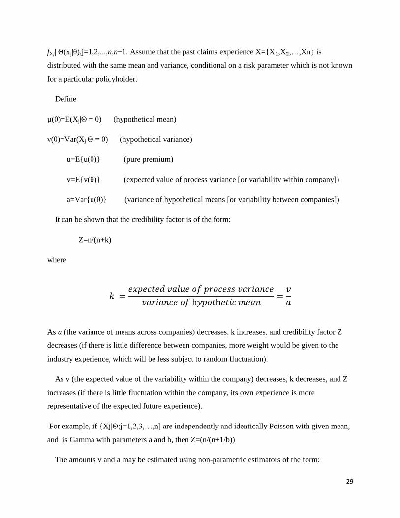
Define

µ(θ)=E(Xj|Θ = θ) (hypothetical mean)

v(θ)=Var(Xj|Θ = θ) (hypothetical variance)

u=E{u(θ)} (pure premium)

v=E{v(θ)} (expected value of process variance [or variability within company])

a=Var{u(θ)} (variance of hypothetical means [or variability between companies])

It can be shown that the credibility factor is of the form:

Z=n/(n+k)

where

𝑘 =𝑒𝑥𝑝𝑒𝑐𝑡𝑒𝑑 𝑣𝑎𝑙𝑢𝑒 𝑜𝑓 𝑝𝑟𝑜𝑐𝑒𝑠𝑠 𝑣𝑎𝑟𝑖𝑎𝑛𝑐𝑒

𝑣𝑎𝑟𝑖𝑎𝑛𝑐𝑒 𝑜𝑓 h𝑦𝑝𝑜𝑡h𝑒𝑡𝑖𝑐 𝑚𝑒𝑎𝑛=𝑣

𝑎

As 𝑎 (the variance of means across companies) decreases, k increases, and credibility factor Z

decreases (if there is little difference between companies, more weight would be given to the

industry experience, which will be less subject to random fluctuation).

As v (the expected value of the variability within the company) decreases, k decreases, and Z

increases (if there is little fluctuation within the company, its own experience is more

representative of the expected future experience).

For example, if {Xj|Θ;j=1,2,3,…,n] are independently and identically Poisson with given mean,

and is Gamma with parameters a and b, then Z=(n/(n+1/b))

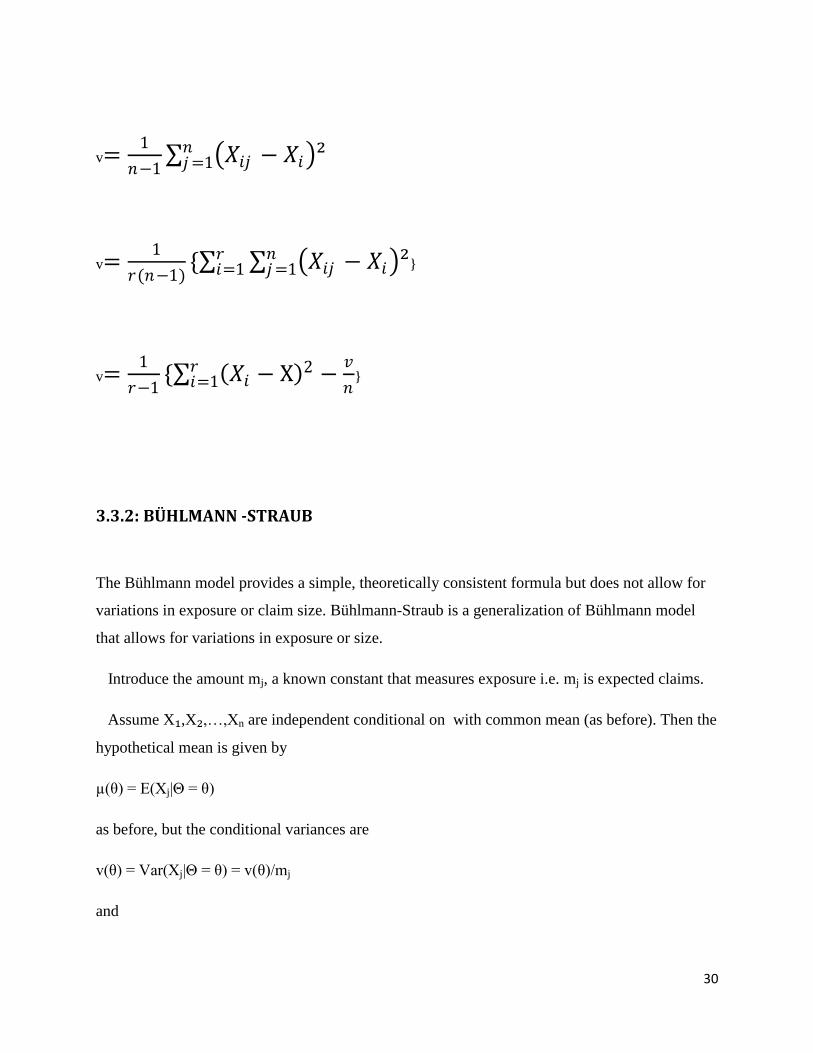
The amounts v and a may be estimated using non-parametric estimators of the form:

30

v=1

𝑛−1 𝑋𝑖𝑗 − 𝑋𝑖 ²𝑛𝑗=1

v=1

𝑟(𝑛−1){ 𝑋𝑖𝑗 − 𝑋𝑖 ²𝑛

𝑗=1𝑟𝑖=1 }

v=1

𝑟−1{ 𝑋𝑖 − X 2𝑟

𝑖=1 −𝑣

𝑛}

3.3.2: BÜHLMANN -STRAUB

The Bühlmann model provides a simple, theoretically consistent formula but does not allow for

variations in exposure or claim size. Bühlmann-Straub is a generalization of Bühlmann model

that allows for variations in exposure or size.

Introduce the amount mj, a known constant that measures exposure i.e. mj is expected claims.

Assume X₁,X₂,…,Xn are independent conditional on with common mean (as before). Then the

hypothetical mean is given by

µ(θ) = E(Xj|Θ = θ)

as before, but the conditional variances are

v(θ) = Var(Xj|Θ = θ) = v(θ)/mj

and

31

Z=m/(m+k)

Where k is same as under the Bühlmann model above and m = sum of all exposure amounts mj

This formula reflects variations in exposure and allows for between company effect and within

company effect.

32

CHAPTER 4

BAYESIAN CREDIBILITY

4.1.1: INTRODUCTION

The relationship between Bayes theorem and credibility was first noticed by Arthur Bailey

(1950) who showed that the formula ZX+(1-Z) can be derived from Bayes theorem, either by

assuming that the number of claims follow a Bernoulli process, with a Beta prior distribution on

the unknown parameter p, or by assuming that the number of claims follow a Poisson process,

with a Gamma prior distribution on the unknown parameter m. (The formula for Z differs,

however, depending on whether a Bernoulli or a Poisson process is assumed.)

The Bayesian approach to credibility involves the following steps:

-- Prior parameter distribution

-- Likelihood function

-- Posterior parameter distribution

-- Loss function

-- Parameter estimate

General advantages of Bayesian Approach

• Bayesian approach conforms to the mathematical theory.

33

• All of the assumptions made are set forth explicitly.

Disadvantages of Bayesian Approach

• All models require the actuary to make assumptions. So, some actuaries might prefer to

employ a different type of prior distribution and/or to use a different set of prior parameters.

- However, when actuaries are updating premium rates, Bayesian approach should be natural.

- Another difficulty is whether a Bayesian approach to the problem is acceptable, and, if so,

what values to assign to the parameters of the prior distribution.

- The last difficulty is that even if the problem fits into a Bayesian framework, the Bayesian

approach may not work in the sense that it may not produce an estimate which can readily be

rearranged to be in the form of a credibility estimate.

This study of the Bayesian approach to credibility theory is illustrated by considering two

models:

-- the Poisson/gamma model which looks at claim frequencies.

-- the normal/normal model which looks at claim amounts.

4.1.2: THE POISSON/GAMMA MODEL

The Gamma-Poisson model has two components:

(1) a Poisson distribution which models the number of claims for an insuredwith a given claims

frequency, and

(2) a Gamma distributionto model the distribution of claim frequencies withina population of

insureds. As in previous sections the goal isto use observations about an insured to infer future

expectations.

34

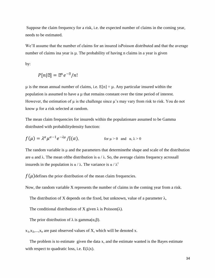
Suppose the claim frequency for a risk, i.e. the expected number of claims in the coming year,

needs to be estimated.

We’ll assume that the number of claims for an insured isPoisson distributed and that the average

number of claims ina year is µ. The probability of having n claims in a year is given

by:

𝑃[𝑛|µ] = µ𝑛𝑒−µ /𝑛!

µ is the mean annual number of claims, i.e. E[n] = µ. Any particular insured within the

population is assumed to have a µ that remains constant over the time period of interest.

However, the estimation of µ is the challenge since µ’s may vary from risk to risk. You do not

know µ for a risk selected at random.

The mean claim frequencies for insureds within the populationare assumed to be Gamma

distributed with probabilitydensity function:

𝑓 𝜇 = 𝜆𝛼𝜇𝛼−1𝑒−𝜆𝜇 / (𝛼) , for µ > 0 and α, λ > 0

The random variable is µ and the parameters that determinethe shape and scale of the distribution

are α and λ. The mean ofthe distribution is α / λ. So, the average claims frequency acrossall

insureds in the population is α / λ. The variance is α / λ2

𝑓 𝜇 defines the prior distribution of the mean claim frequencies.

Now, the random variable X represents the number of claims in the coming year from a risk.

The distribution of X depends on the fixed, but unknown, value of a parameter λ,

The conditional distribution of X given λ is Poisson(λ).

The prior distribution of λ is gamma(α,β).

x₁,x₂,...,xn are past observed values of X, which will be denoted x.

The problem is to estimate given the data x, and the estimate wanted is the Bayes estimate

with respect to quadratic loss, i.e. E(λ|x).

35

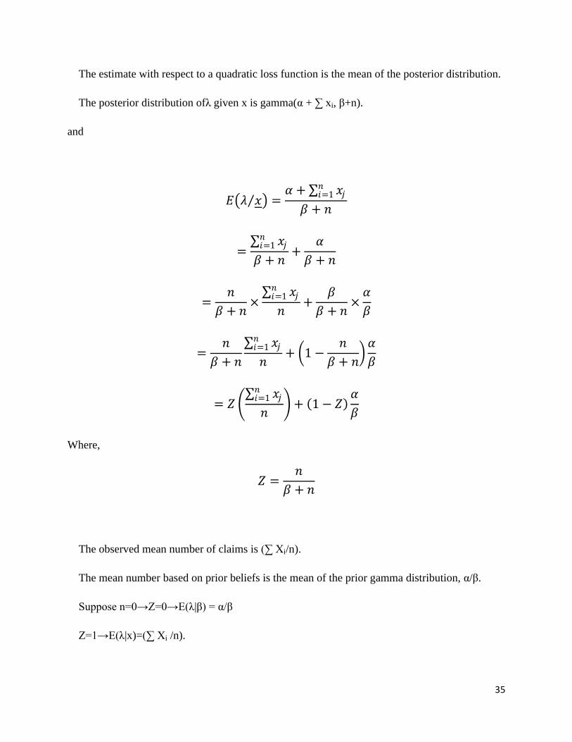
The estimate with respect to a quadratic loss function is the mean of the posterior distribution.

The posterior distribution ofλ given x is gamma(α + ∑ xi, β+n).

and

𝐸 𝜆 𝑥 =𝛼 + 𝑥𝑗

𝑛𝑖=1

𝛽 + 𝑛

= 𝑥𝑗𝑛𝑖=1

𝛽 + 𝑛+

𝛼

𝛽 + 𝑛

=𝑛

𝛽 + 𝑛× 𝑥𝑗𝑛𝑖=1

𝑛+

𝛽

𝛽 + 𝑛×𝛼

𝛽

=𝑛

𝛽 + 𝑛

𝑥𝑗𝑛𝑖=1

𝑛+ 1−

𝑛

𝛽 + 𝑛 𝛼

𝛽

= 𝑍 𝑥𝑗𝑛𝑖=1

𝑛 + 1− 𝑍

𝛼

𝛽

Where,

𝑍 =𝑛

𝛽 + 𝑛

The observed mean number of claims is (∑ Xi/n).

The mean number based on prior beliefs is the mean of the prior gamma distribution, α/β.

Suppose n=0→Z=0→E(λ|β) = α/β

Z=1→E(λ|x)=(∑ Xi /n).

36

The value of Z depends on the amount of data available for the risk, n, and the collateral

information, through β.

As n increases the sampling error of (∑ Xi /n) as an estimate for λ decreases.

β reflects the variance of the prior distribution for .

Thus Z reflects the relative reliability of the two alternative estimates of.

4.1.3: THE NORMAL/NORMAL MODEL

In this section we will estimate the pure premium, i.e. the expected aggregate claims, for a

risk.

Let X be a random variable representing the aggregate claims in the coming year for this risk

and the following assumptions are made:

-- The distribution of X depends on the fixed, but unknown, value of a parameter θ,

-- The conditional distribution of X given θ is N(θ, σ₁²).

-- The uncertainty about the value of θ is modelled in the usual Bayesian way by regarding it

as a random variable.

-- The prior distribution of θ is N(θ, σ₂²).

-- The values of μ ,σ₁² and σ₂² are known.

-- n past values of X have been observed, which will be denoted x.

If the value of were known, the correct pure premium for this risk would be

E(X|θ)= θ

The problem then is to estimate E(X|θ) given x.

37

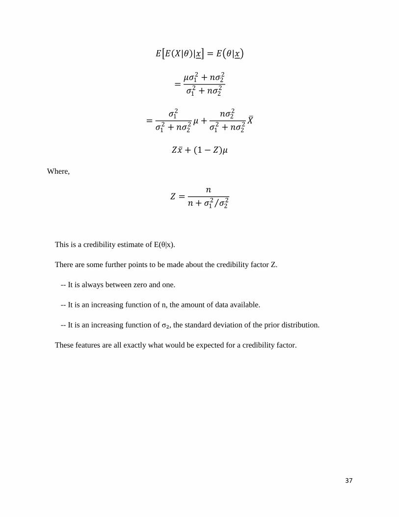
𝐸 𝐸 𝑋|𝜃 |𝑥 = 𝐸 𝜃|𝑥

=𝜇𝜎1

2 + 𝑛𝜎22

𝜎12 + 𝑛𝜎2

2

=𝜎1

2

𝜎12 + 𝑛𝜎2

2 𝜇 +𝑛𝜎2

2

𝜎12 + 𝑛𝜎2

2 𝑋

𝑍𝑥 + (1− 𝑍)𝜇

Where,

𝑍 =𝑛

𝑛 + 𝜎12 𝜎2

2

This is a credibility estimate of E(θ|x).

There are some further points to be made about the credibility factor Z.

-- It is always between zero and one.

-- It is an increasing function of n, the amount of data available.

-- It is an increasing function of σ₂, the standard deviation of the prior distribution.

These features are all exactly what would be expected for a credibility factor.

38

4.2: DISCUSSION OF THE BAYESIAN APPROACH TO CREDIBILITY

The approach used in the Poisson/gamma and normal/normal models was essentially the same.

This approach can be summarized as follows:

-- The problem is stated, e.g. to determine a claim size or claim number distribution. In each

case the aim is to estimate some quantity which characterizes this distribution, e.g. the mean

number of claims or the mean claim size.

-- Some model assumptions are then made within a Bayesian framework, e.g. it is assumed

that the claim number distribution is Poisson and that the unknown parameter of the Poisson

distribution has a gamma distribution with specified parameters.

-- A (Bayesian) estimate of the particular quantity is derived.

-- This estimate is then shown to be in the form of a credibility estimate.

This approach has been very successful in these two cases. It has made the notion of collateral

data very precise (by interpreting it in terms of a prior distribution) and has given formulae for

the calculation of the credibility factor.

The two drawbacks of this approach are:

-- The first difficulty is whether a Bayesian approach to the problem is acceptable, and, if so,

what values to assign to the parameters of the prior distribution.

-- The second difficulty is that even if the problem fits into a Bayesian framework, the

Bayesian approach may not work in the sense that it may not produce an estimate which can

readily be rearranged to be in the form of a credibility estimate.

39

CHAPTER 5

GENERALIZED LINEAR MODELS

5.1: INTRODUCTION

Regression models are used in fitting of insurance claims data. The interest is usually to

look at the relationship between random variables. In the regression analysis, an appropriate

model is chosen and fitted with a view to exploiting the relationship between the variables to

help estimate the expected responses for given values of the explanatory variables. A generalized

linear model (GLM) may be regarded as an extension of a linear model.

The essential difference for GLMs is that we now allow the distribution of the data to be

non-normal. This is particularly important in actuarial work where the data very often do not

have a normal distribution. For example, in mortality, the Poisson distribution is used in

modelling the force of mortality, µx, and the binomial distribution for the initial rate of mortality,

qx. In general insurance, the Poisson distribution is often used for modelling the claim frequency

and the gamma or lognormal distribution for the claim severity.

The main merits of GLMs are twofold. Firstly, regression is no longer restricted to

normal data, but extended to distributions from the exponential family. This enables appropriate

modelling of, for instance, frequency counts, skewed or binary data. Secondly, a GLM models

the additive effect of explanatory variables on a transformation of the mean, instead of the mean

itself.

The aims of a data analysis exercise are usually to decide which variables or factors are

important predictors for the risk being considered, and then to quantify the relationship between

the predictors and the risk in order to assess appropriate premium levels. Our objective covers

the basic theory of GLMswhich is necessary for applications together with credibility theory.

40

GLMs relate a variable (called the response variable) which you want to predict, to

variables or factors (called predictors, covariates or independent variables)about which you have

information. In order to do this, it is necessary first to define the distribution of the response.

Then the covariates can be related to the response allowing for the random variation of the data.

Thus, the first step is to consider the general form of distributions (known as exponential

families) which are used in GLMs.

5.2: METHODOLOGY

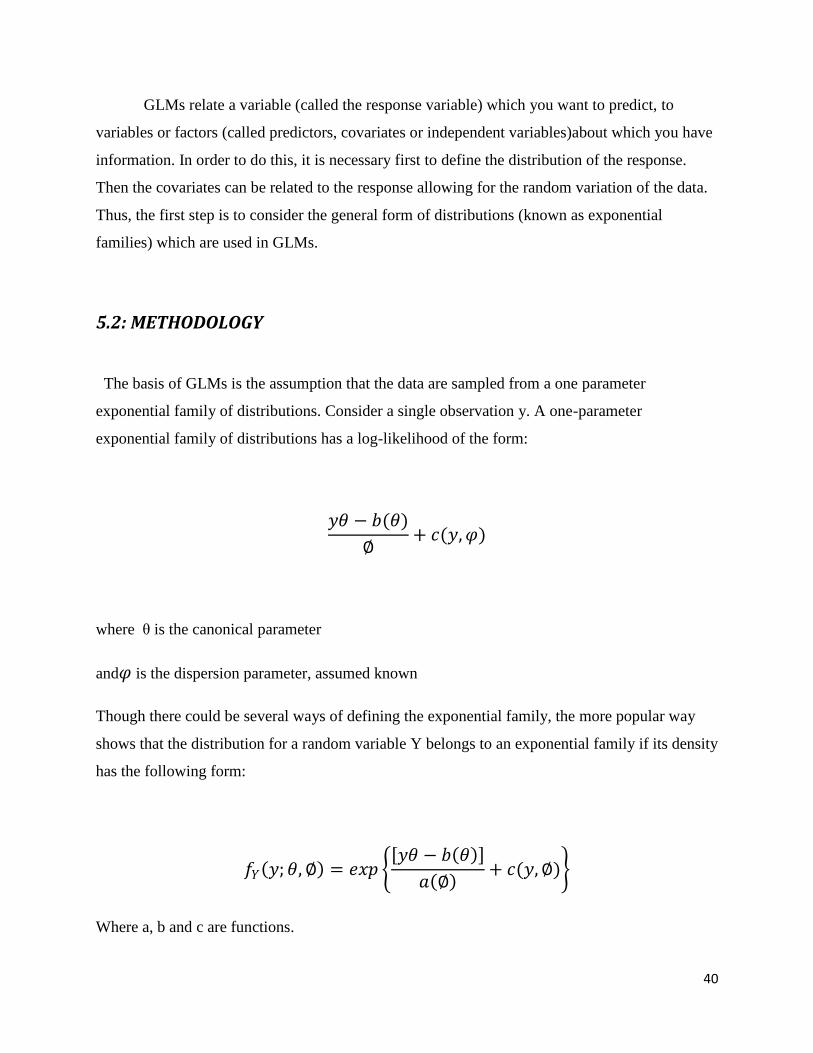
The basis of GLMs is the assumption that the data are sampled from a one parameter

exponential family of distributions. Consider a single observation y. A one-parameter

exponential family of distributions has a log-likelihood of the form:

𝑦𝜃 − 𝑏(𝜃)

∅+ 𝑐(𝑦,𝜑)

where θ is the canonical parameter

and𝜑 is the dispersion parameter, assumed known

Though there could be several ways of defining the exponential family, the more popular way

shows that the distribution for a random variable Y belongs to an exponential family if its density

has the following form:

𝑓𝑌 𝑦;𝜃,∅ = 𝑒𝑥𝑝 𝑦𝜃 − 𝑏 𝜃

𝑎 ∅ + 𝑐(𝑦,∅)

Where a, b and c are functions.

41

Haberrnan and Renshaw (1996) review the application of Generalized Linear Models in actuarial

science, and include a section on loss distributions. In actuarial applications, many distributions

belonging to one-parameter exponential families are useful.

However, Haberman and Renshaw (1996) show how it is also possible to fit certain heavy-tailed

distributions using Generalized Linear Models

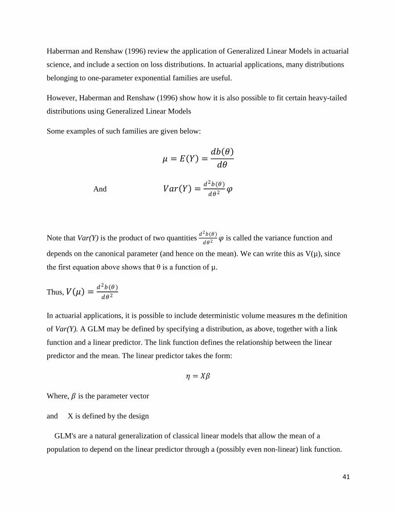
Some examples of such families are given below:

𝜇 = 𝐸 𝑌 =𝑑𝑏 𝜃

𝑑𝜃

And 𝑉𝑎𝑟 𝑌 =𝑑2𝑏(𝜃)

𝑑𝜃2𝜑

Note that Var(Y) is the product of two quantities 𝑑2𝑏(𝜃)

𝑑𝜃2 𝜑 is called the variance function and

depends on the canonical parameter (and hence on the mean). We can write this as V(µ), since

the first equation above shows that θ is a function of µ.

Thus, 𝑉 𝜇 =𝑑2𝑏(𝜃)

𝑑𝜃2

In actuarial applications, it is possible to include deterministic volume measures m the definition

of Var(Y). A GLM may be defined by specifying a distribution, as above, together with a link

function and a linear predictor. The link function defines the relationship between the linear

predictor and the mean. The linear predictor takes the form:

𝜂 = 𝑋𝛽

Where, 𝛽 is the parameter vector

and X is defined by the design

GLM's are a natural generalization of classical linear models that allow the mean of a

population to depend on the linear predictor through a (possibly even non-linear) link function.

42

The generalized linear mixed model is an extension of the GLM, complicated by random

effects.

GLMMs allow the inclusion of normally distributed random effects and have been applied to a

wide variety of statistical problems.

Hierarchical GLM's (HGLM) also allow the inclusion of random effects, but these are not

restricted to be normally distributed.

As mentioned earlier, one of the advantages of GLMs is that regression is no longer restricted to

normal data, but extended to distributions from the exponential family. This property enables

appropriate modeling of e.g. frequency counting, skewed data and binary data. Furthermore, a

GLM models the additive effect of explanatory variables on a transformation of the mean,

instead of the mean itself.

A GLM consists of the following components:

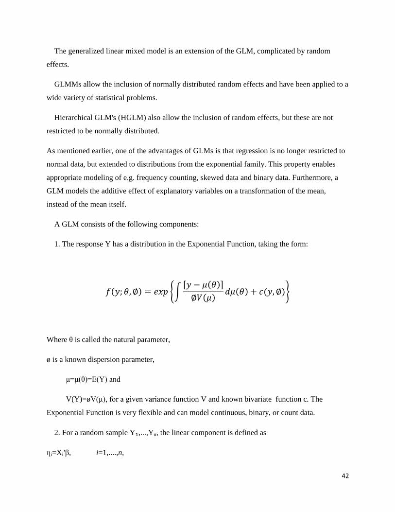
1. The response Y has a distribution in the Exponential Function, taking the form:

𝑓 𝑦;𝜃,∅ = 𝑒𝑥𝑝 𝑦 − 𝜇 𝜃

∅𝑉 𝜇 𝑑𝜇 𝜃 + 𝑐(𝑦,∅)

Where θ is called the natural parameter,

ø is a known dispersion parameter,

μ=μ(θ)=E(Y) and

V(Y)=øV(μ), for a given variance function V and known bivariate function c. The

Exponential Function is very flexible and can model continuous, binary, or count data.

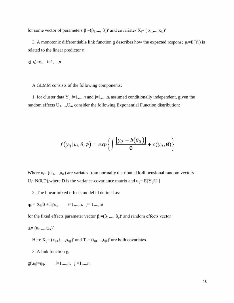
2. For a random sample Y₁,...,Yn, the linear component is defined as

ηi=Xi′β, i=1,....,n,

43

for some vector of parameters β =(β₁,..., βp)′ and covariates Xi= ( xi1,...,xip)′

3. A monotonic differentiable link function g describes how the expected response μi=E(Yi) is

related to the linear predictor ηi

g(µi)=ηi, i=1,...,n.

A GLMM consists of the following components:

1. for cluster data Yij,i=1,...,n and j=1,...,ni assumed conditionally independent, given the

random effects U₁,...,Un, consider the following Exponential Function distribution:

𝑓 𝑦𝑖𝑗 |𝜇𝑖 ,𝜃,∅ = 𝑒𝑥𝑝 𝑦𝑖𝑗 − 𝑏 𝜃𝑖𝑗

∅+ 𝑐(𝑦𝑖𝑗 ,∅)

Where ui= (ui1,...,uik) are variates from normally distributed k-dimensional random vectors

Ui∼N(0,D),where D is the variance-covariance matrix and uij= E[Yij|Ui]

2. The linear mixed effects model id defined as:

ηij = Xij′β +Tij′ui, i=1,...,n, j= 1,...,ni

for the fixed effects parameter vector β =(β₁,..., βp)′ and random effects vector

ui= (ui1,...,uik)′.

Here Xij= (xij1},...,xijp)′ and Tij= (tij1,...,tijk)′ are both covariates.

3. A link function g,

g(µij)=ηij, i=1,...,n, j =1,...,ni

44

completes the model.

For GLM, the Iog-likelihoods for some common distributions are given below

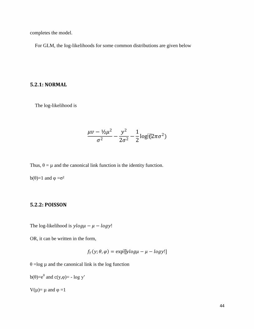
5.2.1: NORMAL

The log-likelihood is

𝜇𝑣 −½𝜇2

𝜎2−𝑦2

2𝜎2−

1

2log(2𝜋𝜎2)

Thus, θ = µ and the canonical link function is the identity function.

b(θ)=1 and φ =σ²

5.2.2: POISSON

The log-likelihood is 𝑦𝑙𝑜𝑔𝜇 − 𝜇 − 𝑙𝑜𝑔𝑦!

OR, it can be written in the form,

𝑓𝑌 𝑦;𝜃,𝜑 = exp[𝑦𝑙𝑜𝑔𝜇 − 𝜇 − 𝑙𝑜𝑔𝑦!]

θ =log µ and the canonical link is the log function

b(θ)=eθ and c(y,φ)= - log y′

V(µ)= µ and φ =1

45

Thus, the natural parameter for the Poisson distribution is logµ, the mean is

E(Y) = b′(θ) = eθ = μ

and the variance function is

V(μ) = b′′(θ) = eθ = μ.

The variance function tells us that the variance is proportional to the mean. We can see that the

variance is actually equal to the mean since a(ϕ) = 1.

5.2.3: BINOMIAL

This is slightly more awkward to deal with, since we have to first divide the binomial random

variable by n.

Thus, suppose R∼Binomial(m,µ). Define Y=(R/m).

The distribution of R is

𝑓𝑅 𝑅;𝜃,𝜑 = 𝑚

𝑅 𝜇𝑅(1− 𝜇)𝑚−𝑅

And by substituting for R, the distribution of Y is

𝑓𝑌 𝑦;𝜃,𝜑 = 𝑚

𝑚𝑦 𝜇𝑚𝑦 (1− 𝜇)𝑚−𝑚𝑦

= exp 𝑚 𝑦𝑙𝑜𝑔𝜇 + 1− 𝑦 log 1− 𝜇 + 𝑙𝑜𝑔 𝑚

𝑚𝑦

= exp 𝑚 𝑦𝑙𝑜𝑔 𝜇

1− 𝜇 + log 1− 𝜇 + 𝑙𝑜𝑔

𝑚

𝑚𝑦

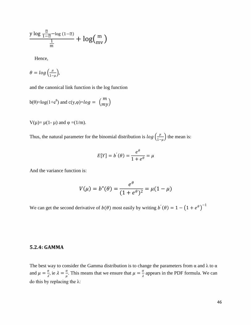
Then the log-likelihood is

46

y log µ1−µ

−log 1−µ

1m

+ log mmv

Hence,

𝜃 = 𝑙𝑜𝑔 𝜇

1−𝜇 ,

and the canonical link function is the log function

b(θ)≈log(1+eθ) and c(y,φ)=𝑙𝑜𝑔 =

𝑚𝑚𝑦

V(µ)= µ(1- µ) and φ =(1/m).

Thus, the natural parameter for the binomial distribution is 𝑙𝑜𝑔 𝜇

1−𝜇 the mean is:

𝐸 𝑌 = 𝑏′ 𝜃 =𝑒𝜃

1 + 𝑒𝜃= 𝜇

And the variance function is:

𝑉 𝜇 = 𝑏"(𝜃) =𝑒𝜃

(1 + 𝑒𝜃)2= 𝜇(1− 𝜇)

We can get the second derivative of 𝑏(𝜃) most easily by writing 𝑏′ 𝜃 = 1 − 1 + 𝑒𝜃 −1

5.2.4: GAMMA

The best way to consider the Gamma distribution is to change the parameters from α and λ to α

and 𝜇 =𝛼

𝜆, ie 𝜆 =

𝛼

𝜇. This means that we ensure that 𝜇 =

𝛼

𝜆 appears in the PDF formula. We can

do this by replacing the λ:

47

𝑓𝑌 𝑦;𝜃,𝜑 =𝜆𝛼

ᴦ(𝛼)𝑦𝛼−1𝑒−𝜆𝑦

=𝛼𝛼

𝜇𝛼ᴦ(𝛼)𝑦𝛼−1𝑒−𝑦𝛼 /𝜇

= 𝑒𝑥𝑝 −𝑦

𝜇− 𝑙𝑜𝑔𝜇 𝛼 + 𝛼 − 1 𝑙𝑜𝑔𝑦 + 𝛼𝑙𝑜𝑔𝛼 − logᴦ(𝛼)

The log-likelihood is

−𝑦

µ+𝑙𝑜𝑔 1

µ

1

𝑣

+ 𝑣𝑙𝑜𝑔𝑦 + 𝑣𝑙𝑜𝑔𝑣 − 𝑙𝑜𝑔⎾ (𝑣)

𝜃 = −1

𝜇

and the canonical link as the reciprocal function.

𝜑 = 𝛼

𝑎 𝜑 =1

𝜑

𝑏(𝜃) = − 𝑙𝑜𝑔(−𝜃)

and c(y,φ)=vlog y+vlog v – log (𝑣) .

V(µ)= µ² and φ =v⁻¹.

Thus, the natural parameter for the gamma distribution is 1

𝜇, ignoring the minus

sign.

The mean is:

48

𝐸 𝑌 𝑏′ 𝜃 = −1

𝜃= 𝜇

The variance function is:

𝑉 𝜇 = 𝑏" (𝜃 ) =1

𝜃2= 𝜇2

And so the variance is 𝜇2

𝛼.

5.3: HGLMS AND BÜHLMANN-STRAUB CREDIBILITY MODEL

Nelder and Verrall (1997) showed how credibility theory takes part in HGLMs by the help of

Bühlmann credibility theory. Basically, when positive weights stemming from difference in

model assumptions are taken into consideration, a credibility formula like that in Buhlmann

model can be formed by using HGLM for Buhlmann-Straub.

We have data for i=1,2,…,n; let t=1,2,…,Ti be described as 𝑦𝑖𝑡 and assume that Ti=s for every i.

thus i index the risks within the collective. In credibility theory, it is assumed that each risk has a

risk parameter and this parameter for risk i is defined as θi.

Let it be assumed that 𝑦𝑖𝑡 |𝜃𝑖 is distributed according to an exponential family.

Define 𝜇 𝜃𝑖 = 𝐸 𝑦𝑖𝑡 𝜃𝑖 . Note that 𝐸 𝑦𝑖𝑡 𝜃𝑖 does not depend on t. in this case, the canonical

parameter for observation yit will not depend on t. so, let it be assumed that the statement can be

written as follows:

∅′ 𝑖 = ∅ 𝜇 𝜃𝑖 = ∅ 𝛼𝑖

Here, ∅ is the canonical link function and 𝛼𝑖 is a random effect for ith

group or insured. Thus, it

is 𝜇 𝜃𝑖 = 𝛼𝑖 for standard credibility model. If it is defined that 𝑣𝑖 = ∅ 𝛼𝑖 , then the following

equation is obtained:

∅𝑖′ = 𝑣𝑖

49

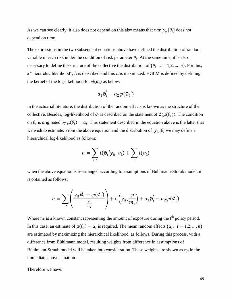
As we can see clearly, it also does not depend on this also means that 𝑣𝑎𝑟[𝑦𝑖𝑡 |𝜃𝑖] does not

depend on t too.

The expressions in the two subsequent equations above have defined the distribution of random

variable in each risk under the condition of risk parameter 𝜃𝑖 . At the same time, it is also

necessary to define the structure of the collective the distribution of {𝜃𝑖 𝑖 = 1,2,… , 𝑛}. For this,

a “hierarchic likelihood”, 𝑕 is described and this 𝑕 is maximized. HGLM is defined by defining

the kernel of the log-likelihood for ∅(𝛼𝑖) as below:

𝑎1∅𝑖′ − 𝑎2𝜑(∅𝑖 ′)

In the actuarial literature, the distribution of the random effects is known as the structure of the

collective. Besides, log-likelihood of 𝜃𝑖 is described on the statement of ∅(𝜇(𝜃𝑖)). The condition

on 𝜃𝑖 is originated by 𝜇 𝜃𝑖 = 𝛼𝑖 . This statement described in the equation above is the latter that

we wish to estimate. From the above equation and the distribution of 𝑦𝑖𝑡 |𝜃𝑖 we may define a

hierarchical log-likelihood as follows:

𝑕 = 𝑙 ∅𝑖 ′𝑦𝑖𝑡 |𝑣𝑖 + 𝑙(𝑣𝑖)

𝑖𝑖 ,𝑡

when the above equation is re-arranged according to assumptions of Bühlmann-Straub model, it

is obtained as follows:

𝑕 = 𝑦𝑖𝑡∅𝑖 − 𝜑 ∅𝑖

𝜑

𝑚 𝑡

𝑖 ,𝑡

+ 𝑐 𝑦𝑖𝑡 ,𝜑

𝑚𝑡 + 𝑎1∅𝑖

′ − 𝑎2𝜑 ∅𝑖′

Where mt is a known constant representing the amount of exposure during the tth

policy period.

In this case, an estimate of 𝜇 𝜃𝑖 = 𝛼𝑖 is required. The mean random effects {𝛼𝑖 : 𝑖 = 1,2,… ,𝑛}

are estimated by maximizing the hierarchical likelihood, as follows. During this process, with a

difference from Bühlmann model, resulting weights from difference in assumptions of

Bühlmann-Straub model will be taken into consideration. These weights are shown as mt in the

immediate above equation.

Therefore we have:

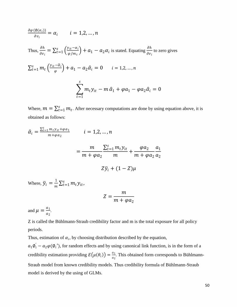
50

𝜕𝜑 (∅(𝛼𝑖))

𝜕𝑣𝑖= 𝛼𝑖 𝑖 = 1,2,… ,𝑛

Thus, 𝜕𝑕

𝜕𝑣𝑖=

𝑦 𝑖𝑡−𝛼𝑖

𝜑/𝑚 𝑡 +𝑠

𝑡=1 𝑎1 − 𝑎2𝛼𝑖 is stated. Equating 𝜕𝑕

𝜕𝑣𝑖 to zero gives

𝑚𝑡 𝑦 𝑖𝑡−𝛼 𝑖

𝜑 +𝑠

𝑡=1 𝑎1 − 𝑎2𝛼 𝑖 = 0 𝑖 = 1,2,… , 𝑛

𝑚𝑡𝑦𝑖𝑡 −𝑚

𝑠

𝑡=1

𝛼 1 + 𝜑𝑎1 − 𝜑𝑎2𝛼 𝑖 = 0

Where, 𝑚 = 𝑚𝑡𝑠𝑡=1 . After necessary computations are done by using equation above, it is

obtained as follows:

𝛼 𝑖 = 𝑚 𝑡𝑦 𝑖𝑡+𝑠𝑡=1 𝜑𝑎1

𝑚+𝜑𝑎2 𝑖 = 1,2,… ,𝑛

=𝑚

𝑚 + 𝜑𝑎2

𝑚𝑡𝑦𝑖𝑡𝑠𝑡=1

𝑚+

𝜑𝑎2

𝑚 + 𝜑𝑎2

𝑎1

𝑎2

𝑍𝑦 𝑖 + (1− 𝑍)𝜇

Where, 𝑦 𝑖 =1

𝑚 𝑚𝑡𝑦𝑖𝑡𝑠𝑡=1 ,

𝑍 =𝑚

𝑚 + 𝜑𝑎2

and 𝜇 =𝑎1

𝑎2.

Z is called the Bühlmann-Straub credibility factor and m is the total exposure for all policy

periods.

Thus, estimation of 𝛼𝑖 , by choosing distribution described by the equation,

𝑎1∅𝑖′ − 𝑎2𝜑(∅𝑖 ′), for random effects and by using canonical link function, is in the form of a

credibility estimation providing 𝐸 𝜇 𝜃𝑖 =𝑎1

𝑎2. This obtained form corresponds to Bühlmann-

Straub model from known credibility models. Thus credibility formula of Bühlmann-Straub

model is derived by the using of GLMs.

51

CHAPTER 6

CONCLUSIONS AND RECOMMENDATIONS

The idea of credibility theory is to up-date the premium charged according to the experience

of the insured entity and the size of the experience. The basic concept of Credibility Theory

has been described, together with the standard methods of finding the Credibility factor. The

connection between Generalized Linear Models and Credibility Theory has been looked at.

The area of Credibility Theory is a backbone of Actuarial studies and so should be

emphasized in the industry especially in dealing with claims experience. Data is not usually

just normal and therefore GLMs are a very important tool in dealing with Credibility Theory.

One major reason of bringing in GLMs into this study is that they give or contribute a further

range of models which may be useful in a wide range of actuarial applications. In summary,

the findings of this study are that Credibility theory is an excellent method to devising a way

of combining the experience of a group with the experience of the individual the better to

calculate the premium.

52

REFERENCES

AITKIN, M., ANDERSON, D., FRANCIS, B and HINDE, J. (1989) StatisticalModelling in GLIM.

Oxford Science Publications, Oxford.

ANTONIO, K. AND J. BEIRLANT, (2006).Actuarial statistics with generalized linear mixed

models.Insurance: Mathematics and Economics, in press.

BÜHLMANN, H. (1967). Experience Rating and Credibility. ASTIN Bulletin 4(3): 199–207.

BÜHLMANN, H. (1969). Experience rating and credibility II.ASTIN Bulletin, 5, 157-165.

BÜHLMANN, H., AND E. STRAUB.(1970). GlaubgewürdigkeitfürSchadensätze (Credibility for Loss

Ratios).Bulletin of the Swiss Association of Actuaries 70: 111–33. (English translation by C. E. Brooks.)

DEMIDENKO, E. (2004). Mixed models: Theory and Applications.Wiley Series in Probability and

Statistics, Hoboken, New Jersey.

DOBSON, A. (1990) An Introduction to Generalized Linear Models. Chapman and Hall, London.

FREES, E.W., (2003). Multivariate credibility for aggregate loss models.North American Actuarial

Journal7, 13–37.

GOOVAERTS, M.J. AND HOOGSTAD, W.J. (1987): Credibility Theory. Survey of Actuarial Studies

No. 4, Nationale-Nederlanden N.V.

GOULET, V., A. FORGUES AND J. LU, (2006). Credibility for severity revisited. North American

Actuarial Journal 10, 49–62.

HABERMAN, S. & RENSHAW, A.E. (1996).Generalized linear models and actuarial science.The

Statistician, 45(4), 407-436.

HACHEMEISTER, C.A. (1975). Credibility for regression models with application to trend. Appeared

in:Credibility, theory and application., Proceedings of the Berkeley Actuarial Research Conference

oncredibility, Academic Press, New York, 129-163.

JEWELL, W.S. (1974). Credible means are exact Bayesian for exponential families. ASTIN Bulletin, 8,

336-341.

KLUGMAN, S (1987) Credibility for classification Ratemaking via the Hierachical Normal Linear

Model Proc of the Casualty Act Soc. 74. 272-321

53

KLUGMAN, S.A. (1992). Bayesian statistics in actuarial science with emphasis on credibility. Kluwer,

Boston.

MAKOV, U., SMITH, A.F.M. & LIU, Y.H. (1996).Bayesian methods in actuarial science.The

Statistician, 45(4), 503-515.

MCCULLAGH, P. & NELDER, J.A. (1989).Generalized linear models.Monographs on statistics

andapplied probability, Chapman and Hall, New York.

MCCULLOCH, C.E. & SEARLE, S.R. (2001).Generalized, Linear and Mixed Models.Wiley Series in

Probability and Statistics, Wiley New York.

MOWBRAY, A. H. 1914. How Extensive a Payroll Exposure is Necessary to Give a Dependable Pure

Premium? Proceedings of the Casualty Actuarial Society 1: 25–30.

Nelder, J.A. &Verrall, R.J. (1997).Credibility theory and generalized linear models.ASTIN

Bulletin,27(1), 71-82.

WHITNEY, A. W. 1918. The Theory of Experience Rating. Proceedings of the Casualty Actuarial Society

4: 275–93.

ZEHWIRTH (1977) The mean credibility formula is a Bayes rule Scandinavian Actuarial Journal, 4.

212-216