On the Axiomatization of the Satiation and Habit

Formation Utility Models

Ying He†, James S. Dyer†, John C. Butler* Department of Information, Risk, and Operational Management†

Department of Finance* McCombs School of Business, University of Texas at Austin

ying.he08irom@utexas.edu, j.dyer@mccombs.utexas.edu, butlerjc@mccombs.utexas.edu

Abstract: We propose a preference condition called shifted difference independence to model the

reference point dependent measurable time preference. Based on this condition, we axiomatize a

general habit formation and satiation model (GHS) to capture both effects of habit formation and

satiation. This model allows for a general habit formation function and satiation function that contain

the functional forms in the existing literature as special cases. Since the GHS model can be reduced to

either a general satiation model (GSa) or a general habit formation model (GHa), our theory also

provides approaches to axiomatize both the GSa model and the GHa model. Furthermore, by adding

extra preference conditions into our axiomatization framework, we axiomatize a GHS model with a

linear habit formation function and a recursively defined linear satiation function. Finally, we show

that the idea developed in this paper also applies to the axiomatization of these models for risky time

preference.

Key words: time preference; habit formation; satiation; axiomatization; discounted utility; measurable

preference

1. Introduction

The discounted utility (DU) model proposed by Samuelson (1937) has been a dominant model of

intertemporal choice for about half a century. One of the main reasons can be attributed to the seminal

work by Koopmans (1960) who showed that the model could be derived from a set of appealing

axioms. However, even Samuelson and Koopmans had some reservations about the descriptive

validity of the model (Frederick et al 2002). There have been a number of documented experiments

challenging the validity of the DU model as a descriptive model in the last two decades (Frederick et

al 2002). One of the primary mechanisms to improve the descriptive validity of the DU model is to

relax the independence axiom to allow the past consumption experience to influence the experienced

utility derived from the current consumption. Prior consumption could influence preference over

current and future consumption in two distinct ways: habit formation and satiation (Reed et al 1999).

2

During the last few decades, several models have been proposed to capture the effect of habit

formation on the utility derived from consumption (experienced utility) in each period (e.g. Pollak

1970, Wathieu 1997, Carroll et al 2000). Recently, Rozen (2010) axiomatized a habit formation model

with linear habit functions over an infinite time horizon, which placed the model on a solid

foundation.

The satiation effect on intertemporal utility function has been modeled by relatively few studies

compared to habit formation (Bell 1974, Baucells and Sarin 2007). Satiation captures the

psychological phenomenon that people may feel fully satisfied by previous consumption, so

additional consumption of the commodity in the current period provides very little incremental utility.

In short, habit formation may cause people to become addicted to a previously consumed commodity,

while satiation may lead to boredom due to previous consumption. Each effect results from different

influences of the past consumption experience on current and future consumption

On the basis of these two models, Baucell and Sarin (2010) proposed a hybrid model of habit

formation and satiation (HS) that combines the influence of both effects of past consumption on the

experienced utility in each period. This model assumes the overall utility from a consumption stream

can be represented by the following function.

����, … , ��� = � ����[���� + �� − ℎ�� − �����]����

In the above utility function, �� = �����, … ����� and ℎ� = ℎ����, … ����� are functions representing the satiation level and habit level in period � respectively, both of which depend on the past consumptions stream ��, ��, … , ����. Baucells and Sarin (2010) also assumed specific functional forms for �� and ℎ�. In their concluding remarks, they identified the need for future research efforts to axiomatize the habit formation (Ha) and satiation (Sa) model.

In this paper, we propose a hierarchy of axioms to develop a General Habit Formation and

Satiation (GHS) model that can be reduced to either a General Satiation (GSa) model or a General

Habit Formation (GHa) model. These general models allow more flexible functional forms for the

satiation function �� and the habit formation function ℎ�. By assuming further restrictive axioms, we obtain models with a recursively defined linear satiation function and a linear habit function. The

main axiom used in this paper defines the shifted independence condition, which is motivated by the

notion of reference dependent preferences that has been studied extensively in psychology, economics,

behavioral decision making, and management science (Kahneman and Tversky 1979, Bell 1982,

Loomes and Sugden 1982, Loewenstein 1988, Tversky and Kahneman 1991, Köszegi and Rabin 2006,

3

Bleichrodt 2007, Apesteguia and Ballester 2009). The mathematical form of the habit formation

model axiomatized in this paper is similar to the model axiomatized by Rozen (2010), but the

behavioral assumptions underlying the preference conditions are different. In Rozen’s theory, the main

axiom is based on the concept of compensation for the consumption, while the main axiom in our

paper is based on the shifting of the reference point against which future consumption is compared.

Our GHS model is axiomatized over a finite horizon which is consistent Wathieu’s (1997) assertion

that it is essential for the habit formation model to be finite (see section 3).

The rest of the paper is organized as follows. In section 2, we formally define the main

preference condition used to axiomatize the models in a measurable preference context, which we

refer to as the shifted difference independence condition, and discuss the implication of this condition.

In section 3, we axiomatize a General Satiation (GSa) model, which contains Baucells and Sarin’s

satiation model (2007) and Bell’s intertemporal preference model (1974) as special cases. Section 4

focuses on the axiomatization of the General Habit Formation and Satiation (GHS) model. Section 5

discusses the more restrictive axioms that support the linear satiation and habit functions. In section 6,

we discuss how our theory can be applied to axiomatize these models in a risky preference context.

Section 7 concludes the paper. All the proofs are provided in the appendix.

2. Shifted difference independence for a measurable value function

We denote a two period consumption stream by ���, ��� ∈ �� × ��, where the consumption space in each period is the real set, i.e. ��: = ! and ��: = !. We assume a measurable preference order (Krantz et al. 1971, Dyer and Sarin 1979) over the set of consumption streams �� × �� denoted by ≿# with an associated strength of preference order denoted by ≿∗. Following the notation of Dyer and Sarin (1979), the expression �%, &��', (� ≿∗ �), *���, +� means that the strength of preference for the exchange from �', (� to �%, &� is greater than or equal to that from ��, +� to �), *�. The measurable value function representing this order is denoted by ,���, ���.

To motivate our new preference condition, let us first consider the following example for

consumption over two time periods. Assume a new cupcake vendor has opened near your office. You

are asked to evaluate streams of cupcake consumption over two days. You may feel that your

preference for consumption on day 2 may be influenced by your consumption on day 1. To obtain

more insight into your preference for cupcake consumption, you can compare a pair of consumption

exchanges: �0,2� vs. �0,3� and �2,2� vs. �2,3�. In the first exchange, you plan to consume �0,2� but you have an opportunity to exchange it for �0,3�; in the second exchange, you plan to consume

4

�2,2� but you have an opportunity to exchange it for �2,3�. After considering the two situations, you ask yourself whether the value increase from the first exchange is larger or smaller than that from the

second exchange. The answer to this question may be different in the following three cases.

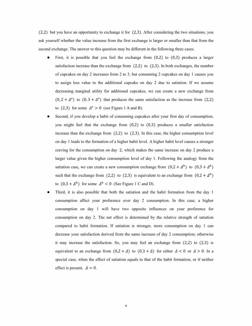
� First, it is possible that you feel the exchange from �0,2� to �0,3� produces a larger satisfaction increase than the exchange from �2,2� to �2,3�. In both exchanges, the number of cupcakes on day 2 increases from 2 to 3, but consuming 2 cupcakes on day 1 causes you

to assign less value to the additional cupcake on day 2 due to satiation. If we assume

decreasing marginal utility for additional cupcakes, we can create a new exchange from

�0, 2 + /0� to �0, 3 + /0� that produces the same satisfaction as the increase from �2,2� to �2,3� for some /0 > 0 (see Figure 1 A and B).

� Second, if you develop a habit of consuming cupcakes after your first day of consumption,

you might feel that the exchange from �0,2� to �0,3� produces a smaller satisfaction increase than the exchange from �2,2� to �2,3�. In this case, the higher consumption level on day 1 leads to the formation of a higher habit level. A higher habit level causes a stronger

craving for the consumption on day 2, which makes the same increase on day 2 produce a larger value given the higher consumption level of day 1. Following the analogy from the

satiation case, we can create a new consumption exchange from �0,2 + /2� to �0,3 + /2� such that the exchange from �2,2� to �2,3� is equivalent to an exchange from �0,2 + /2� to �0,3 + /2� for some /2 < 0 (See Figure 1 C and D).

� Third, it is also possible that both the satiation and the habit formation from the day 1

consumption affect your preference over day 2 consumption. In this case, a higher

consumption on day 1 will have two opposite influences on your preference for

consumption on day 2. The net effect is determined by the relative strength of satiation

compared to habit formation. If satiation is stronger, more consumption on day 1 can

decrease your satisfaction derived from the same increase of day 2 consumption; otherwise

it may increase the satisfaction. So, you may feel an exchange from �2,2� to �2,3� is equivalent to an exchange from �0,2 + /� to �0,3 + /� for either / < 0 or / > 0. In a special case, when the effect of satiation equals to that of the habit formation, or if neither

effect is present, / = 0.

5

Figure 1. Adjustment of reference point under satiation and habit formation

After verifying the existence of the / adjustment on the reference point in the above example, if you can further determine that the / produced by satiation and habit formation only depends on the consumption level on day 1 and is independent of the increase in consumption on day 2, your

measurable preference satisfies a more general condition called shifted difference independence

which we formalize as follows.

Definition 1. �� is said to be shifted difference independent of �� if for any %, 5 ∈ ��, there

exists /�%, 5� ∈ ! such that for any (, & ∈ ��, �%, &��%, (� ∼∗ 75, & + /�%, 5�875, ( + /�%, 5�8.

This condition captures all three of the cases discussed in the example above. When /�%, 5� is equal to zero, shifted difference independence is reduced to the difference independence condition

(Dyer and Sarin 1979), which implies an additive multiattribute value function. Difference

independence also implies weak difference independence (Dyer and Sarin 1979), which ensures that

,�0,3� − ,�0,2�

,�0, ���

�� 2 3

,�2,3� − ,�2,2�= ,�0,3 + /2�− ,�0,2 + /2�

,�0, ���

�� 2

3

,�2, ��� C D

Habit Formation

/2

Reference point

/2>0

,�2,3� − ,�2,2�= ,�0,3 + /0�− ,�0,2 + /0� ,�0,3� − ,�0,2�

,�0, ���

�� 2 3

,�0, ���

�� 2

3 /0

,�2, ��� A B

Satiation

Reference point

/0 > 0

6

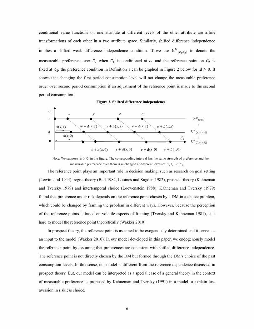
conditional value functions on one attribute at different levels of the other attribute are affine

transformations of each other in a two attribute space. Similarly, shifted difference independence

implies a shifted weak difference independence condition. If we use ≿#�:;,:<� to denote the measureable preference over �� when �� is conditioned at �� and the reference point on �� is fixed at ��, the preference condition in Definition 1 can be graphed in Figure 2 below for / > 0. It shows that changing the first period consumption level will not change the measurable preference

order over second period consumption if an adjustment of the reference point is made to the second

period consumption.

Figure 2. Shifted difference independence

Note: We suppose / > 0 in the figure. The corresponding interval has the same strength of preference and the measurable preference over them is unchanged at different levels of %, 5, 0 ∈ ��.

The reference point plays an important role in decision making, such as research on goal setting

(Lewin et al 1944), regret theory (Bell 1982, Loomes and Sugden 1982), prospect theory (Kahneman

and Tversky 1979) and intertemporal choice (Loewenstein 1988). Kahneman and Tversky (1979)

found that preference under risk depends on the reference point chosen by a DM in a choice problem,

which could be changed by framing the problem in different ways. However, because the perception

of the reference points is based on volatile aspects of framing (Tversky and Kahneman 1981), it is

hard to model the reference point theoretically (Wakker 2010).

In prospect theory, the reference point is assumed to be exogenously determined and it serves as

an input to the model (Wakker 2010). In our model developed in this paper, we endogenously model

the reference point by assuming that preferences are consistent with shifted difference independence.

The reference point is not directly chosen by the DM but formed through the DM’s choice of the past

consumption levels. In this sense, our model is different from the reference dependence discussed in

prospect theory. But, our model can be interpreted as a special case of a general theory in the context

of measurable preference as proposed by Kahneman and Tversky (1991) in a model to explain loss

aversion in riskless choice.

%

0 �� /�%, 0�

* = & (

( + /�%, 0� & + /�%, 0� = + /�%, 0� * + /�%, 0�

��

5 ( + /�%, 5� & + /�%, 5� = + /�%, 5� * + /�%, 5� /�%, 5� ≿#�>,?�

≿#�?,@�>,?�� ≿#�A,@�>,A��

= =

7

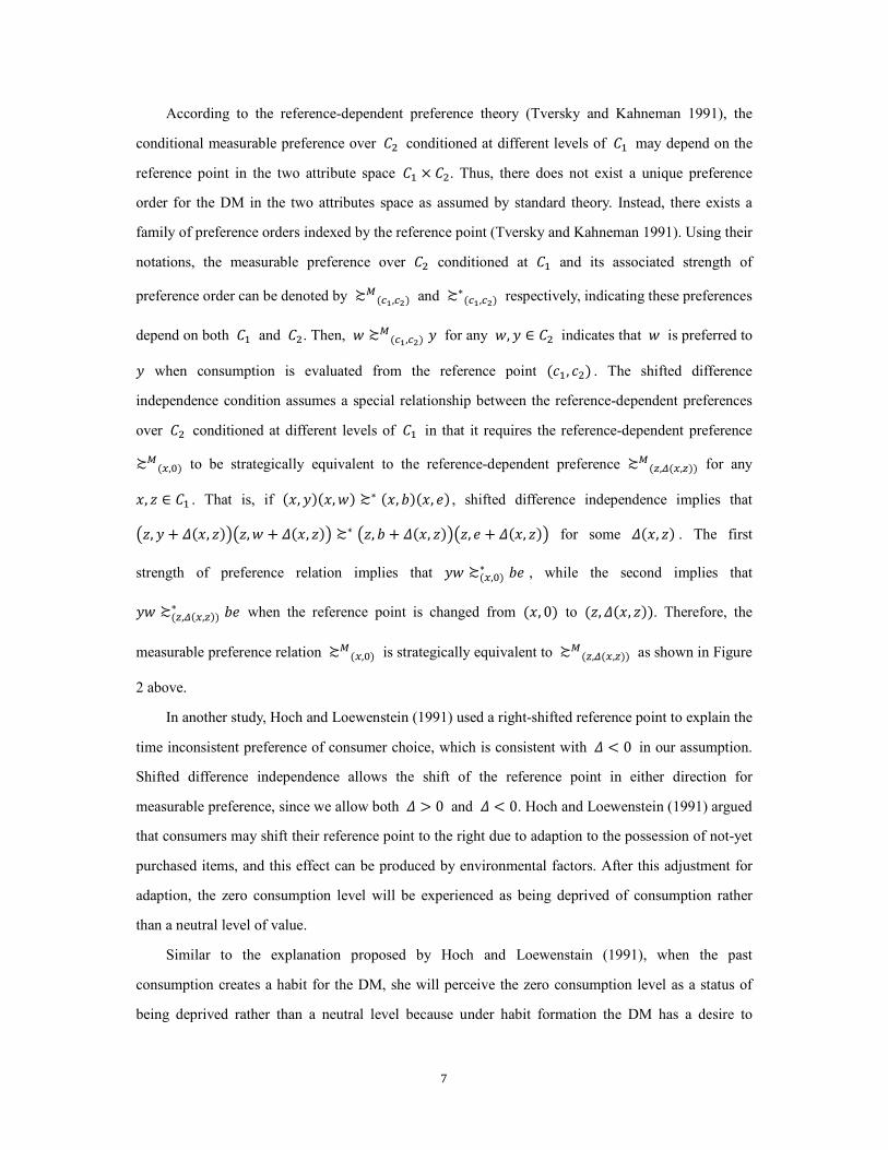
According to the reference-dependent preference theory (Tversky and Kahneman 1991), the

conditional measurable preference over �� conditioned at different levels of �� may depend on the reference point in the two attribute space �� × ��. Thus, there does not exist a unique preference order for the DM in the two attributes space as assumed by standard theory. Instead, there exists a

family of preference orders indexed by the reference point (Tversky and Kahneman 1991). Using their

notations, the measurable preference over �� conditioned at �� and its associated strength of preference order can be denoted by ≿#�:;,:<� and ≿∗�:;,:<� respectively, indicating these preferences depend on both �� and ��. Then, ( ≿#�:;,:<� & for any (, & ∈ �� indicates that ( is preferred to & when consumption is evaluated from the reference point ���, ��� . The shifted difference independence condition assumes a special relationship between the reference-dependent preferences

over �� conditioned at different levels of �� in that it requires the reference-dependent preference ≿#�>,?� to be strategically equivalent to the reference-dependent preference ≿#�A,@�>,A�� for any %, 5 ∈ �� . That is, if �%, &��%, (� ≿∗ �%, *��%, =� , shifted difference independence implies that 75, & + /�%, 5�875, ( + /�%, 5�8 ≿∗ 75, * + /�%, 5�875, = + /�%, 5�8 for some /�%, 5� . The first strength of preference relation implies that &( ≿�>,?�∗ *= , while the second implies that &( ≿�A,@�>,A��∗ *= when the reference point is changed from �%, 0� to �5, /�%, 5��. Therefore, the measurable preference relation ≿#�>,?� is strategically equivalent to ≿#�A,@�>,A�� as shown in Figure 2 above.

In another study, Hoch and Loewenstein (1991) used a right-shifted reference point to explain the

time inconsistent preference of consumer choice, which is consistent with / < 0 in our assumption. Shifted difference independence allows the shift of the reference point in either direction for

measurable preference, since we allow both / > 0 and / < 0. Hoch and Loewenstein (1991) argued that consumers may shift their reference point to the right due to adaption to the possession of not-yet

purchased items, and this effect can be produced by environmental factors. After this adjustment for

adaption, the zero consumption level will be experienced as being deprived of consumption rather

than a neutral level of value.

Similar to the explanation proposed by Hoch and Loewenstain (1991), when the past

consumption creates a habit for the DM, she will perceive the zero consumption level as a status of

being deprived rather than a neutral level because under habit formation the DM has a desire to

8

maintain a certain amount of consumption. This perception of zero consumption as deprivation is

consistent with a right shift of the reference point. For a left shift, we argue that a similar mechanism

also exists due to satiation. Under satiation, the past consumption may spill over into the current and

future periods and the decision maker may experience utility of zero consumption above the neutral

utility level consistent with an endowed consumption from the past. This endowed consumption can

make the DM feel as if she has already consumed an amount of the commodity due to her positive

past consumption. Because of this endowed consumption, the DM may become bored leading to

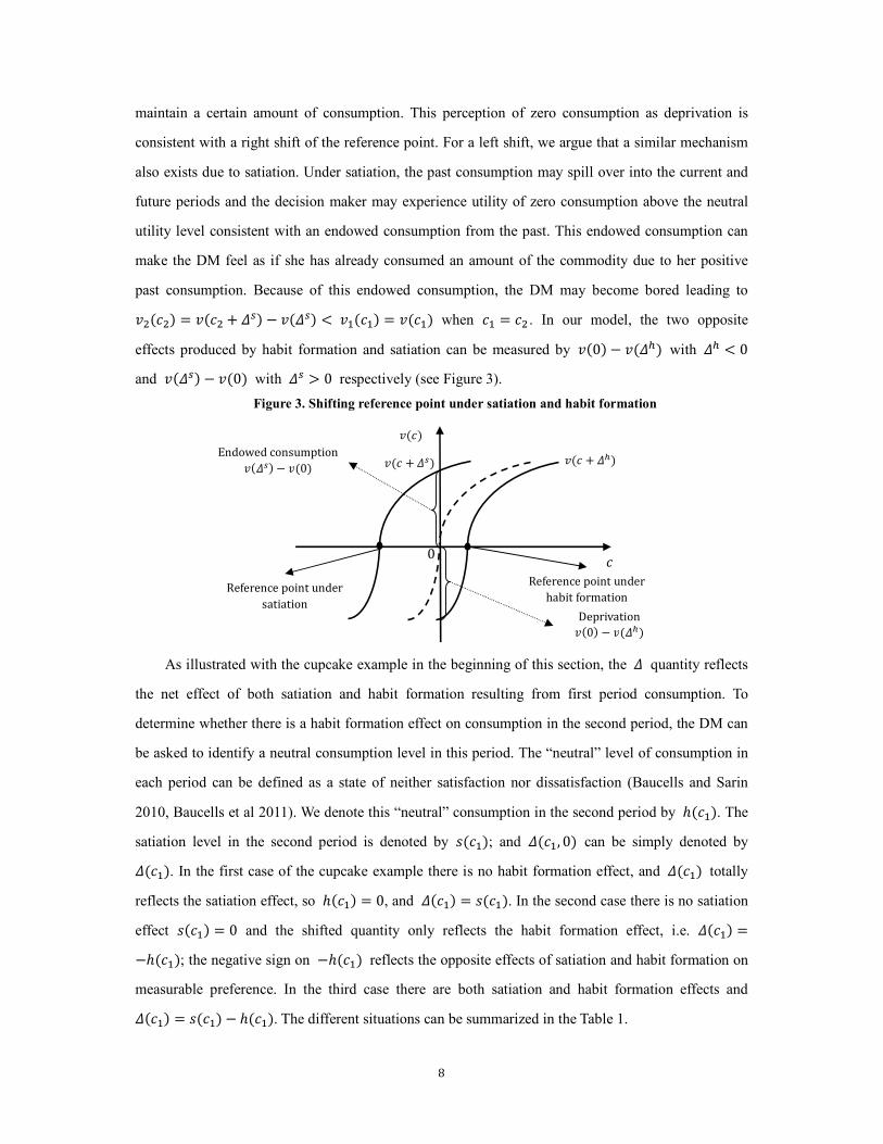
,����� = ,��� + /0� − ,�/0� < ,����� = ,���� when �� = �� . In our model, the two opposite effects produced by habit formation and satiation can be measured by ,�0� − ,�/2� with /2 < 0 and ,�/0� − ,�0� with /0 > 0 respectively (see Figure 3).

Figure 3. Shifting reference point under satiation and habit formation

As illustrated with the cupcake example in the beginning of this section, the / quantity reflects the net effect of both satiation and habit formation resulting from first period consumption. To

determine whether there is a habit formation effect on consumption in the second period, the DM can

be asked to identify a neutral consumption level in this period. The “neutral” level of consumption in

each period can be defined as a state of neither satisfaction nor dissatisfaction (Baucells and Sarin

2010, Baucells et al 2011). We denote this “neutral” consumption in the second period by ℎ����. The satiation level in the second period is denoted by �����; and /���, 0� can be simply denoted by /����. In the first case of the cupcake example there is no habit formation effect, and /���� totally reflects the satiation effect, so ℎ���� = 0, and /���� = �����. In the second case there is no satiation effect ����� = 0 and the shifted quantity only reflects the habit formation effect, i.e. /���� =−ℎ����; the negative sign on −ℎ���� reflects the opposite effects of satiation and habit formation on measurable preference. In the third case there are both satiation and habit formation effects and

/���� = ����� − ℎ����. The different situations can be summarized in the Table 1.

�

,�� + /0� ,�� + /2� ,�/0� − ,�0� Endowed consumption

,�0� − ,�/2� Deprivation

0 Reference point under habit formation Reference point under satiation

,���

9

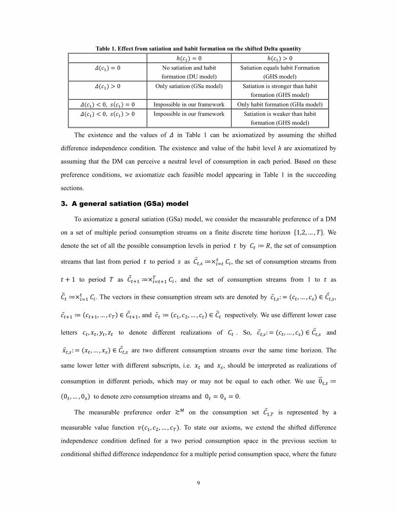
Table 1. Effect from satiation and habit formation on the shifted Delta quantity

ℎ���� = 0 ℎ���� > 0 /���� = 0 No satiation and habit

formation (DU model)

Satiation equals habit Formation

(GHS model) /���� > 0 Only satiation (GSa model) Satiation is stronger than habit

formation (GHS model) /���� < 0, ����� = 0 Impossible in our framework Only habit formation (GHa model) /���� < 0, ����� > 0 Impossible in our framework Satiation is weaker than habit

formation (GHS model)

The existence and the values of / in Table 1 can be axiomatized by assuming the shifted difference independence condition. The existence and value of the habit level h are axiomatized by

assuming that the DM can perceive a neutral level of consumption in each period. Based on these

preference conditions, we axiomatize each feasible model appearing in Table 1 in the succeeding

sections.

3. A general satiation (GSa) model

To axiomatize a general satiation (GSa) model, we consider the measurable preference of a DM

on a set of multiple period consumption streams on a finite discrete time horizon Z1,2, … , \]. We denote the set of all the possible consumption levels in period � by �� ≔ !, the set of consumption streams that last from period � to period � as �_�,0 ≔×`��0 �`, the set of consumption streams from � + 1 to period \ as �_�a� ≔×`��a�� �` , and the set of consumption streams from 1 to � as �b� ≔×`��� �`. The vectors in these consumption stream sets are denoted by �_�,0: = ��� , … , �0� ∈ �_�,0, �_�a� ≔ ���a�, … , ��� ∈ �_�a�, and �b� ≔ ���, ��, … , ��� ∈ �b� respectively. We use different lower case letters �� , %� , &� , 5� to denote different realizations of �� . So, �_�,0: = ��� , … , �0� ∈ �_�,0 and %_�,0: = �%� , … , %0� ∈ �_�,0 are two different consumption streams over the same time horizon. The same lower letter with different subscripts, i.e. %� and %0, should be interpreted as realizations of consumption in different periods, which may or may not be equal to each other. We use 0c_�,0 ≔�0� , … , 00� to denote zero consumption streams and 0� = 00 = 0.

The measurable preference order ≿# on the consumption set �_�,� is represented by a measurable value function ,���, ��, … , ���. To state our axioms, we extend the shifted difference independence condition defined for a two period consumption space in the previous section to

conditional shifted difference independence for a multiple period consumption space, where the future

10

consumption is conditioned at a specific level when we make an adjustment on the reference point.

Definition 2. �� is said to be conditional shifted difference independent of �b��� given

�_�a� = �_�a�, if for any %b���, 5b��� ∈ �b��� there exists /��%b���, 5b���� ∈ �� such that ∀ (� , &� ∈ ��, �%b���, &� , �_�a���%b���, (� , �_�a�� ∼∗ �5b���, &� + /��%b���, 5b����, �_�a���5b���, (� + /��%b���, 5b����, �_�a��.

Now, we present our first axiom for the GSa model.

Axiom 1. (Satiation) For any � ∈ Z2, … , \], �� is conditional shifted difference independent

of �b��� with /� ≥ 0 given that �_�a� = 0c_�a�.

This axiom says that given zero consumption levels in the future, the past consumption levels

produce an effect on the strength of preference at time � only through shifting the reference point of the preference at period � to the left. Conditioning the strength of preference comparison on zero future consumption levels allows the possibility of non-negative consumption streams of different

length. For a cupcake consumption problem similar to the one in section 2 with more than two

consumption periods, this axiom assumes that when any period is evaluated as the last period of a

consumption stream, the changes in the previous consumption levels affect the preference over the

last period consumption by shifting its reference point according to the magnitude of the previous

changes. For a DM whose preference satisfies the two period condition described in the cupcake

example in section 2, it is likely that her preference may also satisfy the condition assumed in this

axiom if she believes that extending a two period choice problem to a three (or more) period horizon

would not change the way she compares the consumption streams.

By shifting the reference point to the left, the DM evaluates the consumption in the last period on

a flatter part of the value function. The shifting amount in this axiom works as a satiation level which

depends on the past consumption: the more you feel satiated from past consumption, the less you

evaluate the same consumption in the last period of your consumption stream. In the Appendix, we

show that by assuming the existence of satiation for the last consumption period in this axiom we can

recursively prove the existence of satiation for all previous periods.

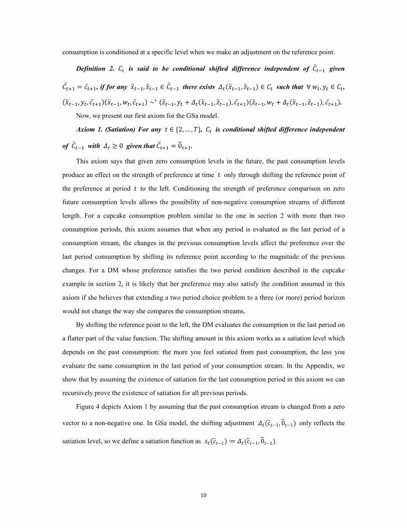
Figure 4 depicts Axiom 1 by assuming that the past consumption stream is changed from a zero

vector to a non-negative one. In GSa model, the shifting adjustment /���b�−1, 0bc�−1� only reflects the satiation level, so we define a satiation function as ����b�−1� ≔ /���b�−1, 0bc�−1�.

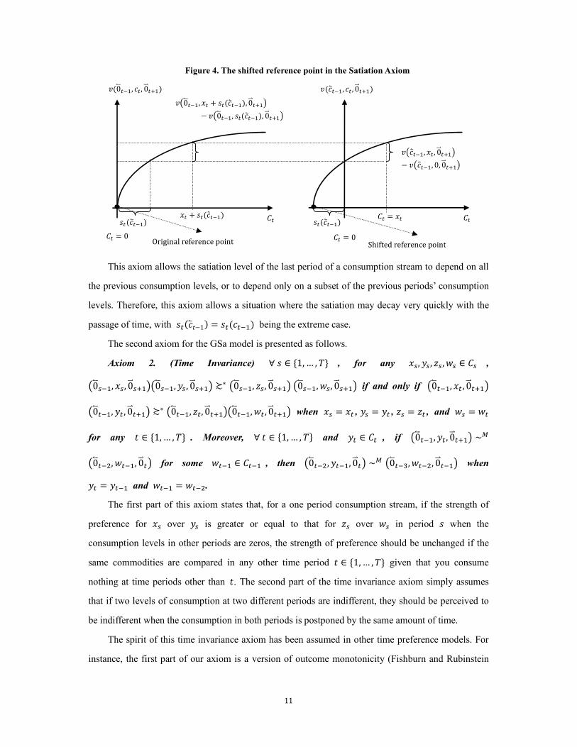
11

Figure 4. The shifted reference point in the Satiation Axiom

This axiom allows the satiation level of the last period of a consumption stream to depend on all

the previous consumption levels, or to depend only on a subset of the previous periods’ consumption

levels. Therefore, this axiom allows a situation where the satiation may decay very quickly with the

passage of time, with ����b�−1� = �������� being the extreme case. The second axiom for the GSa model is presented as follows.

Axiom 2. (Time Invariance) ∀ � ∈ Z1, … , \] , for any %0, &0, 50, (0 ∈ �0 ,

70bc0��, %0, 0c_0a�870bc0��, &0 , 0c_0a�8 ≿∗ 70bc0��, 50, 0c_0a�8 70bc0��, (0, 0c_0a�8 if and only if 70bc���, %� , 0c_�a�8 70bc���, &� , 0c_�a�8 ≿∗ 70bc���, 5�, 0c_�a�870bc���, (� , 0c_�a�8 when %0 = %� , &0 = &� , 50 = 5� , and (0 = (� for any � ∈ Z1, … , \] . Moreover, ∀ � ∈ Z1, … , \] and &� ∈ �� , if 70bc���, &� , 0c_�a�8 ∼# 70bc���, (���, 0c_�8 for some (��� ∈ ���� , then 70bc���, &���, 0c_�8 ∼# 70bc��f, (���, 0c_���8 when

&� = &��� and (��� = (���. The first part of this axiom states that, for a one period consumption stream, if the strength of

preference for %0 over &0 is greater or equal to that for 50 over (0 in period � when the consumption levels in other periods are zeros, the strength of preference should be unchanged if the

same commodities are compared in any other time period � ∈ Z1, … , \] given that you consume nothing at time periods other than �. The second part of the time invariance axiom simply assumes that if two levels of consumption at two different periods are indifferent, they should be perceived to

be indifferent when the consumption in both periods is postponed by the same amount of time.

The spirit of this time invariance axiom has been assumed in other time preference models. For

instance, the first part of our axiom is a version of outcome monotonicity (Fishburn and Rubinstein

,�0bc���, ��, 0c_�a��

�� �� = 0

,��b���, �� , 0c_�a��

�� �� = 0

,7�b���, %� , 0c_�a�8− ,7�b���, 0, 0c_�a�8

�� = %�

,70bc���, %� + ����b����, 0c_�a�8− ,70bc���, ����b����, 0c_�a�8

����b���� ����b���� %� + ����b���� Shifted reference point Original reference point

12

1982, Baucells and Heukamp 2011) in the context of measurable value functions. The second part is

similar to the assumption of stationarity of preference (Fishburn and Rubinstein 1982, Baucells and

Heukamp 2011).

Finally, the third axiom is about the impatience of preferences.

Axiom 3. (Impatience) For any � = Z1, … , \ − 1] when (� = (�a� for some (� ∈ �� and

(�a� ∈ ��a�, 70bc���, (� , 0c_�a�8 ≿# 70bc� , (�a�, 0c_�a�8. This impatience axiom is also called time monotonicity and allows the discounting of the value

function in each period in the model. Fishburn and Rubinstein (1982) and Baucells and Heukamp

(2011) also assume impatience.

Based on the above three axioms, we can show that there exists a general satiation (GSa) model

for the value function ,���, ��, … , ��� over all possible consumption profiles. Theorem 1. Axioms 1, 2, and 3 hold if and only if the measurable preference ≿# over the

consumption streams �b� can be represented by the following model, with � ∈ [0,1] ,���, ��, … , ��� = � ����[,7�� + ����b����8 − ,7����b����8]�

��� where ����b����: �b��� → !l? is called the satiation function with ��70bc���8 = 0 and ����b?� = 0.

Other models in the literature are special cases of this more general satiation model (GSa). When

the satiation function ����b���� is always zero, i.e., ����b���� = 0, the above model is equivalent to the DU model proposed by Koopmans (1960). When ����b���� = m�������b���� + �����, the GSa model is reduced to the Satiation Model (Sa) proposed by Baucells and Sarin (2007). When

����b���� = ������b���� + ����, the GSa is equivalent to the model proposed by Bell (1974). 4. A general habit formation and satiation (GHS) model

As previously discussed, satiation reflects the intuition that past consumption makes the DM

experience less satisfaction from current period consumption because of decreasing marginal utility.

Comparatively, habit formation reflects the possibility that past consumption can make the DM

addicted to the commodity. Baucells and Sarin (2010) proposed a hybrid model of habit formation and

satiation (HS), which inherits the characteristics from both the satiation model and the habit formation

model. In this section, we propose axioms that are necessary and sufficient for a general habit

formation and satiation (GHS) model.

We consider a horizon with n as the life time of a DM. In this horizon, past consumption

13

experience can develop into a consumption habit which has an influence on the experienced utility. In

general, the habit formed could last for any number of possible periods that are limited by the life

horizon. It is possible that the habit can be “reset” (Wathieu, 1997) or changed for some reason, either

subjective or objective, such that it only takes effect on finite periods. For instance, a technology

advance may change the habit of the consumption when consumers switch to a new product. For

example, the availability of the electronic reader, such as the Kindle by Amazon or the iPad by Apple,

may make the DM suddenly switch from a paper version of New York Times to an electronic version.

For some other commodities, the time periods that a habit could last may be shorter. A DM who likes

cupcakes in her lunch may have cupcakes for four or five days, but after that she may want to switch

to another type of dessert. Besides the fact that a habit may only last to a finite time period, Wathieu

(1997) also argues that a DM may only focus on a finite period as the decision window, where the

number of the periods subject to the habit formation effect is called DM’s degree of myopia. In this

paper, we refer to the number of periods the habit formation have an effect in the model as a habit

horizon and use this concept to account for exogenous reasons that influence the length of time a habit

could last.

Under the assumption of the existence of different habit horizons, two consumption streams with

the same consumption levels in each period could be perceived differently by a DM if the habit

horizons are different for each consumption stream. For instance, if the habit formed from the past

consumption lasts to a certain period �, the DM will perceive zero consumption of the commodity in this period as deprivation as it is below the neutral level. However, if the habit horizon is less than �, which means the past consumption does not have a habit formation effect on the experienced utility in

the period �, a zero consumption level at this period is perceived as neutral. We need a richer set of consumption streams to accommodate the impact of the different habit horizons on preference.

Specifically, we use 0o to denote a zero consumption level in a period if the habit horizon does not last to this period. So, for a three period life horizon, ���, ��, 0o f) denotes the consumption stream with zero consumption in the third period and a two period habit horizon; while ���, ��, 0f) denotes a consumption stream with the same consumption levels in each period but with a three period habit

horizon. These two consumption streams could be perceived differently in the habit formation

context.

Formally, on a life horizon with n periods, we denote a consumption stream with a � period habit horizon with non-negative consumption levels up to period � and zero levels after period � by

14

p�b� , 0oc_�a�q : = ���, ��, … , �� , 0o �a�, … , 0o r). Comparatively, a consumption stream with a � + 1 period habit horizon with non-negative consumption levels up to period � and zero levels after period � is denoted by p�b� , 0�a�, 0oc_�a�q : = ���, ��, … , �� , 0�a�, 0o �a�, … , 0o r). The set of all consumption streams of these types are denoted by �b� × 0oc_�a� and �b� × 0� × 0oc_�a� respectively. For simplicity, we also denote �_�,r: =×`��r �` by �br × 0oc_ra� since there are no habits after n periods by the definition of the lifetime. Now, we define a set of consumption streams which contains all the streams in the sets

�b� × 0oc_�a� for any � ∈ Z1,2 … , n] by ℋ ≔ t �b� × 0oc_�a� | ∀ � ∈ Z1, … , n]v . We assume that there exists a measurable preference order ≿# on this set ℋ which is

represented by a measurable value function ,: ℋ → ! . This assumption implies that for any �b��� ∈ �b���, there exists ℎ���b����: �b��� → !l? such that p�b���, ℎ���b����, 0oc_�a�q ∼# p�b���, 0o , 0oc_�a�q. The ℎ���b���� is the neutral consumption in period �, which is the habit level formed from the past consumption in our context. If there were no impact of habit formation, the DM should perceive

p�b���, 0� , 0oc_�a�q ∼# p�b���, 0o � , 0oc_�a�q, which implies ℎ���b���� = 0. Now, we present our first axiom for the GHS model.

Axiom 4. (Memorial Stock) For any � ∈ Z2, … , n] , �� is conditional shifted difference

independent of �b��� given that �_�a� = 0oc_�a�. Axiom 4 says that the strength of preference for the last period of any habit horizon is not

changed by changing the past consumption levels from �b��� to %b��� if the reference point of the conditional preference in period � is shifted by /���b���, %b����. Consider a multiple period cupcake consumption example where both satiation and habit formation may impact preferences. The

Memorial Stock axiom assumes that no matter how long the habit horizon may last, the cupcakes

consumed in previous periods will produce an effect on the preference over the cupcakes consumed in

the last period of a habit horizon by shifting the reference point. Although the changes in the past

consumption levels can produce reference point shifts for multiple future consumption periods up to

the end of the habit horizon, the Memorial Stock axiom only dictates how the changes in past

consumption influence the last period of a habit horizon.

In the appendix, we prove that this condition is sufficient to show that all the previous periods of

a habit horizon are also subject to this reference point shift induced by the changes of the past

consumption levels. Again, a DM may think about a simple two-period version of the cupcake

15

example where the habit formed from the first period consumption has an effect on her preference

over the second period through shifting the reference point. If she can verify that this reference point

shift effect exists for the two period case, she may also have reason to believe that her preference

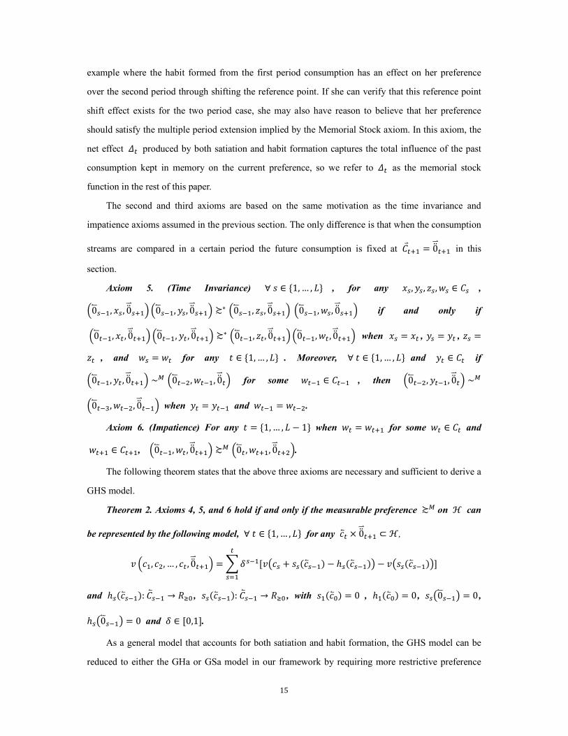
should satisfy the multiple period extension implied by the Memorial Stock axiom. In this axiom, the

net effect /� produced by both satiation and habit formation captures the total influence of the past consumption kept in memory on the current preference, so we refer to /� as the memorial stock function in the rest of this paper.

The second and third axioms are based on the same motivation as the time invariance and

impatience axioms assumed in the previous section. The only difference is that when the consumption

streams are compared in a certain period the future consumption is fixed at �_�a� = 0oc_�a� in this section.

Axiom 5. (Time Invariance) ∀ � ∈ Z1, … , n] , for any %0, &0 , 50, (0 ∈ �0 ,

p0bc0��, %0 , 0oc_0a�q p0bc0��, &0, 0oc_0a�q ≿∗ p0bc0��, 50, 0oc_0a�q p0bc0��, (0, 0oc_0a�q if and only if

p0bc���, %� , 0oc_�a�q p0bc���, &� , 0oc_�a�q ≿∗ p0bc���, 5�, 0oc_�a�q p0bc���, (� , 0oc_�a�q when %0 = %� , &0 = &� , 50 =5� , and (0 = (� for any � ∈ Z1, … , n] . Moreover, ∀ � ∈ Z1, … , n] and &� ∈ �� if

p0bc���, &� , 0oc_�a�q ∼# p0bc���, (���, 0oc_�q for some (��� ∈ ���� , then p0bc���, &���, 0oc_�q ∼# p0bc��f, (���, 0oc_���q when &� = &��� and (��� = (���.

Axiom 6. (Impatience) For any � = Z1, … , n − 1] when (� = (�a� for some (� ∈ �� and

(�a� ∈ ��a�, p0bc���, (� , 0oc_�a�q ≿# p0bc� , (�a�, 0oc_�a�q.

The following theorem states that the above three axioms are necessary and sufficient to derive a

GHS model.

Theorem 2. Axioms 4, 5, and 6 hold if and only if the measurable preference ≿# on ℋ can

be represented by the following model, ∀ � ∈ Z1, … , n] for any �b� × 0oc_�a� ⊂ ℋ,

, p��, ��, … , �� , 0oc_�a�q = � �0��[,7�0 + �0��b0��� − ℎ0��b0���8 − ,7�0��b0���8]�0��

and ℎ0��b0���: �b0�� → !l? , �0��b0���: �b0�� → !l? , with ����b?� = 0 , ℎ���b?� = 0 , �070bc0��8 = 0 ,

ℎ070bc0��8 = 0 and � ∈ [0,1]. As a general model that accounts for both satiation and habit formation, the GHS model can be

reduced to either the GHa or GSa model in our framework by requiring more restrictive preference

16

conditions. From the relation /���b���� = ����b���� − ℎ���b���� , when /���b���� = −ℎ���b���� the satiation ����b���� = 0, and the GHS model is reduced to GHa model.

To see how our GHS model can be reduced to a GSa model, we notice that the main difference in

the settings for the two models in sections 3 and this section is that the consumption set ℋ used in this section is a larger set that contains the consumption set �b� used in section 3. The measurable preference ≿# on this larger set ℋ can be reduced to the measurable preference ≿# on �b� in section 3 when n = \, p%b� , 0c_0,x, 0oc_xa�q ∼# �%b� , 0oc_�a�� for any �, and for any � ∈ Z� + 1, … , n − 1], ' ∈ Z� + 1 , n − 1] with � ≤ ' . If this relationship holds, the different habit horizons do not influence preferences. The axioms in this section are reduced to the corresponding ones in section 3,

and the GHS model is reduced to the GSa model.

5. Linear habit and satiation functions

Linear habit functions have been widely assumed in different habit formation utility models in

the literature (Pollak 1970, Wathieu 1997, Carroll et al 2000). Baucells and Sarin (2007, 2010) also

assume linear functions to model the habit formation and satiation in their models. A linear function is

commonly used to aggregate information on different attributes to make decisions (Dawes and

Corrigan 1974), because it is a robust and tractable functional form. In the context of habit formation

in an infinite horizon, Rozen (2010) proposed a set of axioms that guarantee the existence of a linear

functional form for the habit function. However, we are not aware of any work on this topic in the

context of both habit formation and satiation. In this section, we propose a set of stronger axioms that

specify a linear habit formation and satiation model.

5.1 Linear satiation in GSa model

For the GSa model, we axiomatize a recursively defined linear satiation function given by

����b���� = z��������b���� + ����� for any � by assuming the following axioms. Axiom 7. (Strong Shifted Difference Independence) For any � ∈ Z1, … , \], ∀ �b���, (bcc��� ∈

�b���, ∀ �_�a�, &_�a� ∈ �_�a�, and ∀ �� , &� ∈ ��, there exists a unique {��b���, (bcc���� ∈ �� such that

��b���, ��, �_�a����b���, &� , &_�a�� ∼∗ �(bcc���, �� + {��b���, (bcc����, �_�a���(bcc���, &� + {��b���, (bcc����, &_�a��. This axiom is stronger than the conditional shifted difference independence used in Axiom 1,

which only compares strength of preference over the last period of non zero consumption levels and

assumes that the past consumption experience can only shift the reference point of preference in the

last period. In Axiom 7, the strength of preference is compared in multiple periods. To illustrate, we

17

return to the cupcake example in section 2 with consumption streams of more than two periods; e.g.,

the DM may have a four period consumption stream of cupcakes ���, ��, �f, �|�. For this four period consumption problem, Axiom 7 states that if two consumption streams have the same level in period 1

but differ from period 2 on, the strength of preference over two different streams is unchanged under

different period 1 consumption if the reference point for the conditional preference in period 2 is

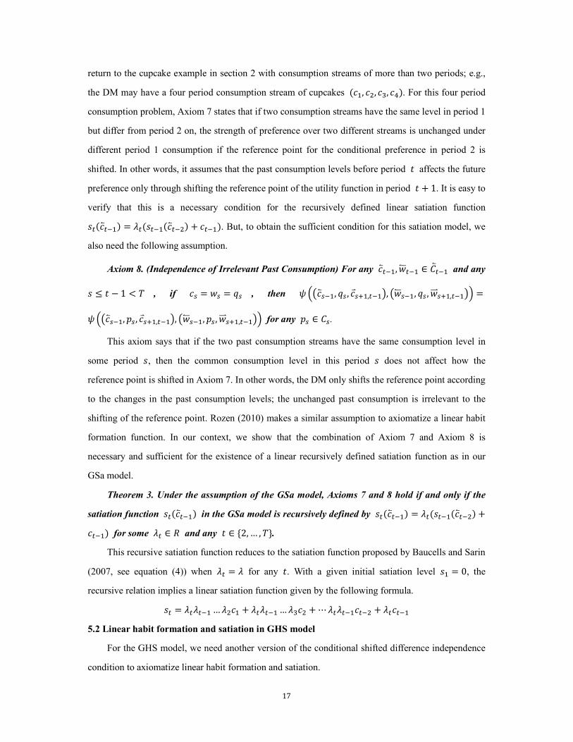
shifted. In other words, it assumes that the past consumption levels before period � affects the future preference only through shifting the reference point of the utility function in period � + 1. It is easy to verify that this is a necessary condition for the recursively defined linear satiation function

����b���� = z��������b���� + �����. But, to obtain the sufficient condition for this satiation model, we also need the following assumption.

Axiom 8. (Independence of Irrelevant Past Consumption) For any �b���, (bcc��� ∈ �b��� and any

� ≤ � − 1 < \ , if �0 = (0 = }0 , then { p7�b0��, }0 , �_0a�,���8, 7(bcc0��, }0 , (cc_0a�,���8q = { p7�b0��, ~0 , �_0a�,���8, 7(bcc0��, ~0 , (cc_0a�,���8q for any ~0 ∈ �0.

This axiom says that if the two past consumption streams have the same consumption level in

some period �, then the common consumption level in this period � does not affect how the reference point is shifted in Axiom 7. In other words, the DM only shifts the reference point according

to the changes in the past consumption levels; the unchanged past consumption is irrelevant to the

shifting of the reference point. Rozen (2010) makes a similar assumption to axiomatize a linear habit

formation function. In our context, we show that the combination of Axiom 7 and Axiom 8 is

necessary and sufficient for the existence of a linear recursively defined satiation function as in our

GSa model.

Theorem 3. Under the assumption of the GSa model, Axioms 7 and 8 hold if and only if the

satiation function ����b���� in the GSa model is recursively defined by ����b���� = z��������b���� +����� for some z� ∈ ! and any � ∈ Z2, … , \].

This recursive satiation function reduces to the satiation function proposed by Baucells and Sarin

(2007, see equation (4)) when z� = z for any �. With a given initial satiation level �� = 0, the recursive relation implies a linear satiation function given by the following formula.

�� = z�z��� … z��� + z�z��� … zf�� + ⋯ z�z������� + z����� 5.2 Linear habit formation and satiation in GHS model

For the GHS model, we need another version of the conditional shifted difference independence

condition to axiomatize linear habit formation and satiation.

18

Axiom 9. (Multiple Period Shifted Difference Independence) For any � ≤ � ∈ Z2, … , n], any

�b���, %b��� ∈ �b��� , and any �_�,0, %_�,0 ∈ �_�,0 , there exists a unique vector {c_�,0�%b���, �b����: =7{��%b���, �b����, {�a��%b���, �b����, … , {0�%b���, �b����8 ∈ �_�,0 such that p%b���, �_�,0, 0oc_0a�q p%b���, %_�,0, 0oc_0a�q ∼∗ p�b���, �_�,0 + {c_�,0�%b���, �b����, 0oc_0a�q p�b���, %_�,0 + {c_�,0�%b���, �b����, 0oc_0a�q.

Axiom 9 is stronger than the Axiom 4 assumed in section 4; when � = �, Axiom 9 reduces to Axiom 4. However, unlike Axiom 4 which assumes that the changes in the past consumption levels

only shift the reference point of the utility function in the last period of a habit horizon, Axiom 9

assumes that these changes can shift the reference points of the utility function in multiple future

periods. In the cupcake example, if there are four periods in a habit horizon, Axiom 9 assumes that the

changes in consumption levels in days 1 and 2 can cause the DM to shift her reference point in both

day 3 and 4 such that her strength of preference over the consumption levels in day 3 and 4 is

unchanged. Furthermore, if the habit horizon is changed, the following axiom assumes that the DM

will shift the reference point in a consistent way for the periods common to both habit horizons.

Axiom 10. (Consistent Shifting) For any �b���, %b��� ∈ �b��� and � < �, ' < n, {c_�,0�%b���, �b���� is equal to {c_�,x�%b���, �b���� from � to ��� Z�, '].

Following the cupcake example, for a five days habit horizon, the changes in the consumption

levels in days 1 and 2 will cause the DM shift her reference points for days 3, 4, and 5. Axiom 10 says

that if identical changes are made in days 1 and 2 for both four day and five day habit horizons, the

shifted quantities in day 3 and 4 should be equal for both habit horizons.

Finally, we also need Axiom 11 assumed below, which shares the same idea for Axiom 8.

Axiom 11. (Independence of Irrelevant Past Consumption) For any �, � < n and �b���, %b��� ∈�b��� and any ' ≤ � − 1, if �x = %x = }x, then {c_�,0 p7%bx��, }x , %_xa�,���8, 7�bx��, }x , �_xa�,���8q ={c_�,0 p7%bx��, ~x , %_xa�,���8, 7�bx��, ~x, �_xa�,���8q for any ~x ∈ �x .

Based on Axioms 9, 10, and 11, the habit function and satiation functions in the GHS model

become linear functions of past consumptions, and the satiation function is recursively defined.

Theorem 4. Under the assumption of the GHS model, Axioms 9, 10 and 11 hold if and only if

the satiation function and memorial stock function are given by the following formulas

����b���� = z��/�����b���� + ����� for some z� ∈ !;

/���b���� = ������ + ������ + ⋯ + ������ + ������ for some �� ∈ !;

19

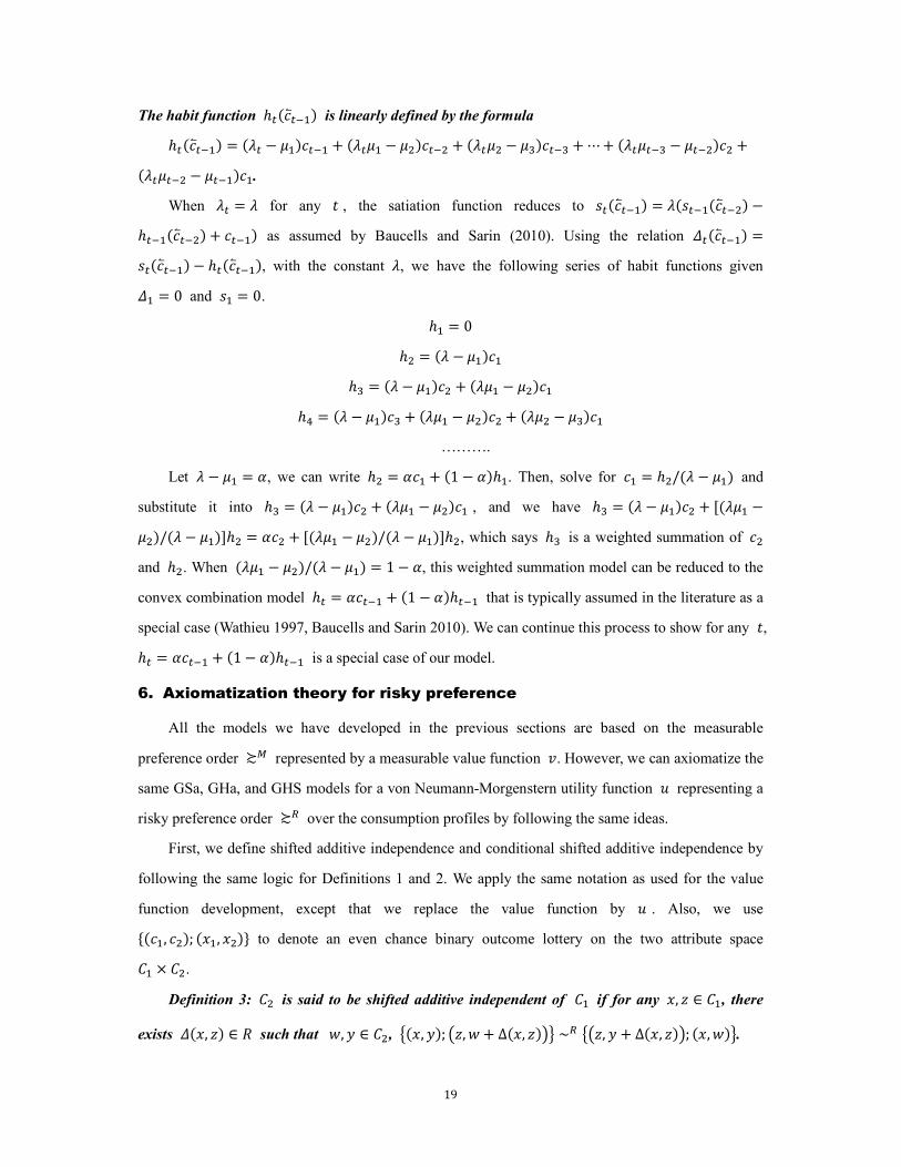
The habit function ℎ���b���� is linearly defined by the formula

ℎ���b���� = �z� − ������� + �z��� − ������� + �z��� − �f����f + ⋯ + �z����f − ������� +�z����� − �������.

When z� = z for any � , the satiation function reduces to ����b���� = z�������b���� −ℎ�����b���� + ����� as assumed by Baucells and Sarin (2010). Using the relation /���b���� =����b���� − ℎ���b����, with the constant z, we have the following series of habit functions given /� = 0 and �� = 0.

ℎ� = 0 ℎ� = �z − ����� ℎf = �z − ����� + �z�� − ����� ℎ| = �z − ����f + �z�� − ����� + �z�� − �f���

……….

Let z − �� = �, we can write ℎ� = ��� + �1 − ��ℎ�. Then, solve for �� = ℎ�/�z − ��� and substitute it into ℎf = �z − ����� + �z�� − ����� , and we have ℎf = �z − ����� + [�z�� −���/�z − ���]ℎ� = ��� + [�z�� − ���/�z − ���]ℎ�, which says ℎf is a weighted summation of �� and ℎ�. When �z�� − ���/�z − ��� = 1 − �, this weighted summation model can be reduced to the convex combination model ℎ� = ����� + �1 − ��ℎ��� that is typically assumed in the literature as a special case (Wathieu 1997, Baucells and Sarin 2010). We can continue this process to show for any �, ℎ� = ����� + �1 − ��ℎ��� is a special case of our model. 6. Axiomatization theory for risky preference

All the models we have developed in the previous sections are based on the measurable

preference order ≿# represented by a measurable value function ,. However, we can axiomatize the same GSa, GHa, and GHS models for a von Neumann-Morgenstern utility function � representing a risky preference order ≿� over the consumption profiles by following the same ideas.

First, we define shifted additive independence and conditional shifted additive independence by

following the same logic for Definitions 1 and 2. We apply the same notation as used for the value

function development, except that we replace the value function by � . Also, we use Z���, ���; �%�, %��] to denote an even chance binary outcome lottery on the two attribute space �� × ��.

Definition 3: �� is said to be shifted additive independent of �� if for any %, 5 ∈ ��, there

exists /�%, 5� ∈ ! such that (, & ∈ ��, ��%, &�; 75, ( + Δ�%, 5�8� ∼� �75, & + Δ�%, 5�8; �%, (��.

20

We can compare this shifted additive independence condition with the additive independence

condition (Fishburn 1965) in the following Figure 5.

Figure 5. Comparison between additive independence and shifted additive independence

Note: the left graph shows the additive independence; the right one shows the shifted additive independence

From Figure 5 above, we can see that shifted additive independence assumes the two even

chance binary lotteries with outcomes on the opposite angles of a parallelogram are indifferent to each

other. When the parallelogram is a rectangle, this condition is reduced to additive independence

(Fishburn 1965).

This condition has the same implication for the utility function as the shifted difference

independence condition has for the measurable value function. Therefore, we can assume similar

axioms for a utility function over consumption steams with more than two periods and duplicate all

the theorems developed in this paper for a utility function �. 7. Conclusion

In this paper, we present a framework to axiomatize a general habit formation and satiation

utility model, which contains many existing models of satiation and habit formation as special cases.

The main axiom used in our framework to derive the model is motivated by the concept of reference

dependent preference which has been extensively studied during the last few decades in economics,

psychology, behavioral decision making, and management science. In general, the reference point is

hard to model theoretically since it is so volatile; and thus a general theory of a reference point has not

been developed (Wakker 2010). However, in the context of intertemporal choice, the preference

conditions proposed in this paper guarantee the existence of an intertemporal utility model where the

reference point in each period is endogenously determined by the previous consumption levels

through habit formation and satiation. Thus, this study contributes to the literature of the reference

��

��

Z�%, &�; �5, (�] ∼� Z�5, &�; �%, (�]

5

%

( & ��

�� %

5

( ( + Δ�%, 5� & & + Δ�%, 5�

Z�%, &�; �5, ( + Δ�%, 5��] ∼� Z75, &+ Δ�%, 5�8; �%, (�]

21

dependent preference research. Moreover, although we also axiomatize the linear satiation and habit

formation functions in this paper, the GHS model admits more general forms of the satiation and habit

formation functions. Finally, the framework in this paper admits the axiomatization for both

measurable preference and risky preference, which are the two types of cardinal preferences

extensively studied in decision making. Therefore, the study in this paper provides theoretical

foundations for a GHS model in both the measurable preference context and the risky preference

context.

Appendix

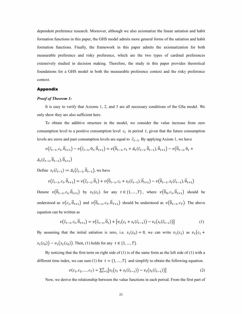
Proof of Theorem 1:

It is easy to verify that Axioms 1, 2, and 3 are all necessary conditions of the GSa model. We

only show they are also sufficient here.

To obtain the additive structure in the model, we consider the value increase from zero

consumption level to a positive consumption level �� in period �, given that the future consumption levels are zeros and past consumption levels are equal to �b���. By applying Axiom 1, we have

,7�b���, �� , 0c_�a�8 − ,7�b���, 0� , 0c_�a�8 = ,70bc���, �� + /���b���, 0bc����, 0c_�a�8 − ,70bc���, 0� +/���b���, 0bc����, 0c_�a�8 Define ����b���� ≔ /�7�b���, 0bc���8, we have

,7�b���, ��, 0c_�a�8 = ,7�b���, 0c_�8 + ,70bc���, �� + ����b����, 0c_�a�8 − ,70bc���, ����b����, 0c_�a�8 Denote ,70bc���, ��, 0c_�a�8 by ,����� for any � ∈ Z1, … , \] , where ,70bc?, ��, 0c_�a�8 should be understood as ,7��, 0c_�a�8 and ,70bc���, �� , 0c_�a�8 should be understood as ,70bc���, ��8. The above equation can be written as

,7�b���, �� , 0c_�a�8 = ,7�b���, 0c_�8 + �,�7�� + ����b����8 − ,�7����b����8� (1) By assuming that the initial satiation is zero, i.e. ����?� = 0, we can write ,����� as ,�7�� +����?�8 − ,�7����?�8. Then, (1) holds for any � ∈ Z1, … , \].

By noticing that the first term on right side of (1) is of the same form as the left side of (1) with a

different time index, we can sum (1) for � = Z1, … , \] and simplify to obtain the following equation. ,���, ��, … , ��� = ∑ �,�7�� + ����b����8 − ,�7����b����8� ���� (2)

Now, we derive the relationship between the value functions in each period. From the first part of

22

Axiom 2, we know for any two periods �, � ∈ Z1, … , \] , the value functions ,� and ,0 are strategically equivalent with each other. So, for any � we have ,���� = �,������ + � and ,������ = �,������ + � for some �, �, �, � ∈ ! . ,��0� = ,�0, … ,0� = 0 for all � implies that � = 0, � = 0. Then, from the second part of Axiom 2 and the affine transformation relationship shown above, we can conclude that for some & there exists ( such that ,��&� = ,����(� =�,����&� and ,����&� = ,����(� = �,����(� for any �. Thus, we can conclude that ,����(� =���,����&� = �,����&�, which implies ��� = �. So, we know for any �, ,���� = �,������.

Denote ,���� by ,���. By applying the relationship ,���� = �,������ for � = Z2, … , \] in (2), we obtain

,���, ��, … , ��� = ∑ �����,7�� + ����b����8 − ,7����b����8�����

Finally, by using Axiom 3, we have ,���� = ����,��� > ,�a���� = ��,��� , which implies ���� > ��, so � ∈ �0,1�.□ Proof of Theorem 2

It is easy to verify that Axioms 4, 5, and 6 are necessary conditions of the GHS model, so we

only verify that they are also sufficient here. The idea of the proof is similar to that used in the proof

of Theorem 1, except that we prove the existence of the habit formation function by using the

definition of the habit level for the value function of each period.

Consider the value increase from zero consumption level to a positive consumption level �� in period �, given that after � there is no habit formation effect and past consumption levels are equal to �b���. By applying Axiom 4, we have

, p�b���, �� , 0oc_�a�q − , p�b���, 0� , 0oc_�a�q= , p0bc���, �� + /���b���, 0bc����, 0oc_�a�q − , p0bc���, 0� + /���b���, 0bc����, 0oc_�a�q

Define /���b����: = /���b���, 0bc���� and ,� = , p0bc���, �� , 0oc_�a�q for � = Z1, … , n], we have , p�b���, �� , 0oc_�a�q = , p�b���, 0� , 0oc_�a�q + ,���� + /���b����� − ,��/���b����� (3) Assuming �� = ℎ���b���� in (3) and defining ����b����: = ℎ���b���� + /���b����, (3) becomes , p�b���, ℎ���b����, 0oc_�a�q = , p�b���, 0� , 0oc_�a�q + ,�7����b����8 − ,��/���b����� (4) By adding and subtracting ,�7����b����8 in (3), we obtain , p�b���, �� , 0oc_�a�q = , p�b���, 0� , 0oc_�a�q + ,�7����b����8 − ,�7/���b����8 + �,�7�� + /���b����8 −

,�7����b����8� (5)

23

Using the definition of ℎ���b���� in the relation p�b���, ℎ���b����, 0oc_�a�q ∼# p�b���, 0oc_�q in section 4, we have , p�b���, ℎ���b����, 0oc_�a�q = , p�b���, 0oc_�q. Replacing , p�b���, ℎ���b����, 0oc_�a�q by , p�b���, 0oc_�q in (4) and substituting it into (5), we have

, p�b���, �� , 0oc_�a�q = , p�b���, 0oc_�q + �,�7�� + ����b���� − ℎ���b����8 − ,�7����b����8� (6) The first term on right side of (6) is of the same form as the left side of (6) with a different time

index. Following the same reasoning used in the proof of Theorem 1, we can obtain the following

additive value function for any habit horizon � ≤ n, where ����b?� = 0 and ℎ���b?� = 0. , p��, ��, … , �� , 0oc_�a�q = ∑ [,07�0 + �0��b0��� − ℎ0��b0���8 − ,07�0��b0���8]�0�� (7)

From Axiom 5, using the same reasoning in the proof of Theorem 1, we can conclude that for

any �, ,0��� = �,0����� and ,0����� = �,0�����. Thus, for any � ∈ Z1, … , �], �b� × 0oc_�a� ∈ �b� ×0oc_�a�, (7) can be written as

, p��, ��, … , �� , 0oc_�a�q = ∑ �0���,7�0 + �0��b0��� − ℎ0��b0���8 − ,7�0��b0���8��0��

Finally, from Axiom 8, we conclude that � ∈ �0,1�.□ Proof of Theorem 3:

To prove Theorem 3, we need Lemmas 1 and 2, which are proved by adapting ideas from Rozen

(2010) to our satiation and habit formation context.

Lemma 1 says that the reference point shifting effect produced by changing the past consumption

from %b��� to 5b��� is equal to the cumulative effect of first changing past consumption from %b��� to &b��� and then from &b��� to 5b���. Lemma 1: (Triangle Equality) ∀ %b��� , &b���, 5b��� ∈ �b��� , {�%b��� , 5b���� = {�%b��� , &b���� +{�&b��� , 5b���� for any �. Proof: Applying Axiom 7, we have

�%b���, ~� , �_�a���%b���, }� , (bcc���� ∼∗ �&b���, ~� + {�%b��� , &b����, �_�a���&b���, }�+ {�%b��� , &b����, (bcc���� ∼∗ �5b���, ~� + {�%b��� , &b���� + {�&b��� , 5b����, �_�a���5b���, }�+ {�%b��� , &b���� + {�&b��� , 5b����, (bcc���� ∼∗ �5b���, ~� + {�%b��� , 5b����, �_�a���5b���, }�+ {�%b��� , 5b����, (bcc���� From the last indifference relation and the uniqueness of the shift quantity assumed in Axiom 7, we

can conclude that {�%b��� , 5b���� = {�%b��� , &b���� + {�&b��� , 5b����. □ Lemma 2 says that the reference point shifting effect produced by a vector of past consumption is

24

the summation of the effects produced by the individual consumption levels in each period.

Lemma 2. (Additive Separability) There exists functions ��, ��, … , ����: ! → ! such that

{��b���� ≔ {70bc���, �b���8 = ���������� + ⋯ + ������ + ������. Proof: By iteratively using the triangle equality, we have

{70bc���, �b���8 = {70bc���, ���, 0�, … , 0����8 +{7���, 0�, … , 0����, ���, ��, 0f, … , 0����8 + {7���, ��, 0f … , 0����, ���, ��, �f, 0|, … , 0����8 + ⋯ +{7���, ��, … , ����, 0����, ���, ��, … , ����, �����8 (8) Define ������ ≔ {70bc���, ���, 0�, … , 0����8. Starting from the second term on the right side of

the above equation, we iteratively apply Axiom 8 to replace the common past consumption levels with

zero consumption levels. Then, define �̀ ����`��� ≔ { p70bc`��, 0c_`��8, �0bc`��, �`��, 0c_`�q for � =3, … , �. Substituting �̀ ����`��� into (8), we obtain the additive separable expression for {��b����. □

Now, we prove Theorem 3. The necessary part is easy to verify, so we only show the sufficient

part here.

We first prove {��b���� = −����b���� . For this purpose, we consider a strength of preference relation where only {��b���� and ����b���� appear in the GSa model in period t. Specifically, we consider the relation 7�b���, �� , 0c_�a�87�b���, &� , 0c_�a�8 ∼∗ 7(bcc���, �� + {��b���, (bcc����, 0c_�a�8 7(bcc���, &� + {��b���, (bcc����, 0c_�a�8 assumed by Axiom 7. Under the assumption of the GSa model, this relation can be written as

,7�� + ����b����8 − ,7&� + ����b����8 =,7�� + {��b���, (bcc���� + ���(bcc����8 − ,7&� + {��b���, (bcc���� + ���(bcc����8 (9) The value difference on the left side of (9) reflects a consumption increase from &� + ����b���� to �� + ����b���� while the right hand side reflects an increase from &� + {��b���, (bcc���� + ���(bcc���� to �� + {��b���, (bcc���� + ���(bcc����, both of which are increased by the same amount �� − &�. Since the value function is a concave increasing function, (9) holds if and only if the following equation (10)

holds. Mathematically, this can be verified by taking derivatives with respect to �� (or &�� on both sides of (9) and then applying the monotonicity of ,:���.

{��b���, (bcc���� + ���(bcc���� = ����b���� (10)

25

When �b��� = 0, (10) is reduced to {70bc���, (bcc���8 + ���(bcc���� = 0 . Thus, we have {��b���� ={70bc���, �b���8 = −����b����.

Now, to derive the relationship between ����b���� and ��a���b��, we consider another strength of preference relation assumed by Axiom 7, 7�b���, �� , ��a�, 0c_�a�87�b���, &� , &�a�, 0c_�a�8 ∼∗ 7(bcc���, �� +{��b���, (bcc����, ��a�, 0c_�a�87(bcc���, &� + {��b���, (bcc����, &�a�, 0c_�a�8 , which measures the strength of preference over the different consumption levels in period � and � + 1. As was true in equation (9) the value differences in period � are equal on both sides of the relation, and so its representation in the GSa model can be reduced to

�,7��a� + ��a� ��b���, ���8 − ,7��a� ��b���, ���8� − �,7&�a� + ��a� ��b���, &��8 − ,7��a� ��b���, &��8�= �, p��a� + ��a� 7(bcc���, �� + {��b���, (bcc����8q − , p��a� 7(bcc���, �� + {��b���, (bcc����8q�− �, p&�a� + ��a� 7(bcc���, &� + {��b���, (bcc����8q − , p��a� 7(bcc���, &� + {��b���, (bcc����8q�

By the same logic used above, taking derivatives with respect to ��a� on both sides of the above equation and using the monotonicity of ,>�%�, we obtain the following equation.

��a� ��b���, ��� = ��a� 7(bcc���, �� + {��b���, (bcc����8 (11) From (10), we have {��b���, (bcc���� = ����b���� − ���(bcc����. Substituting this equation into (11),

we obtain

��a� ��b���, ��� = ��a� 7(bcc���, �� + ����b���� − ���(bcc����8 (12) If we set (bcc��� = 0bc��� , (12) becomes ��a� ��b���, ��� = ��a� p0bc���, �� + ����b����q since

��70bc���8 = 0. Now, define ��%� ≔ ��a� 70bc���, %8, we have ��a� ��b���, ��� = �7�� + ����b����8. Finally, from the fact that {��b���� = −����b���� and Lemma 2, we know that ��a���b�� is also

additively separable, and ��a� ��b�� = −{��b�� = −[������ + ⋯ + ������ + ������] . Therefore, ���a���b���, ���/��� should be independent of �b���. Then, from ��a� ��b���, ��� = �7�� + ����b����8, we know that ��&� must be a linear function. Otherwise, ���a���b���, ���/��� will depend on �b���. Thus, for some z�a� ∈ !, ��a� ��b�� = z�a� 7�� + ����b����8.

The above reasoning works for any �, so the �� in the GSa model is a recursively defined linear function. □

Proof of Theorem 4:

26

To prove Theorem 4, we need the following Lemmas 3, 4, 5, and 6. Lemmas 3 and 4 can be

proved by the same idea used to prove Lemmas 1 and 2. We only prove Lemmas 5 and 6 here, which

are proved by adapting the logic from Rozen (2010) to accommodate both satiation and habit

formation.

Lemma 3. Triangle Equality: {c_�,0�%b��� , 5b���� = {c_�,0�%b��� , &b���� + {c_�,0�&b��� , 5b����. Lemma 4. Additive Separability: {�70bc���, �b���8 = ������ + ������ + ⋯ + ���������� .

Lemma 5 says that the shifting effect on reference point produced by changing consumption in

one period from some level } by some non-zero amount � is independent of the level of the starting point of consumption }, when the consumption in the other periods are at zero levels.

To simplify the discussion, we define the notation }b���x : = �0�, … , 0x��, }x , 0xa�, … , 0���� for ' ∈ Z1, … , � − 1]. By this notation, �} + ��bcccccccccccccc���x denotes �0�, … , 0x��, }x + �x, 0xa�, … , 0����. Lemma 5. Weak Invariance: for any } ∈ !, � ∈ !, ' ∈ Z2, … , � − 1], {�7}b���x , �} + ��bcccccccccccccc���x 8 ={�70bc���x , �b���x 8.

To prove the result, we consider a strength of preference relation where the same reference point

shifting effect in period � can be produced either by changing the past consumption levels during periods 1 to � − 1 or by changing the past consumption levels during periods 1 to ' < � − 1. This implies that the reference point shifting effect in period � in this relation only depends on the consumption change before period '. By Axiom 9, this strength of preference relation is of the following form, ∀ ' ∈ Z2, … , � − 1],

70bcx��, }x, 0c_xa�,���, �_�,r870bcx��, }x , 0c_xa�,���, %_�,r8 ∼∗ p~bx��0 , }x + {x70bcx��, ~bx��0 8, 0c_xa�,��� +{c_xa� ,���70bcx��, ~bx��0 8, �_�,r + {c_� ,r70bcx��, ~bx��0 8q p~bx��0 , }x + {x70bcx��, ~bx��0 8, 0c_xa�,��� +{c_xa� ,���70bcx��, ~bx��0 8, %_�,r + {c_� ,r70bcx��, ~bx��0 8q for some � ≤ ' − 1, where we assume the habit horizon is n. The length of the habit horizon does not matter here, as long as we consider a habit horizon with more than � periods.

Now, we treat the first � − 1 periods as past, which implies that the past consumption levels are changed from }b���x = 70bcx��, }x, 0c_xa�,���8 to p~bx��0 , }x + {x70bcx��, ~bx��0 8, {c_xa� ,���70bcx��, ~bx��0 8q in the strength of preference relation. This implies {c_� ,r70bcx��, ~bx��0 8 = {c_� ,r �}b���x , p~bx��0 , }x +{x70bcx��, ~bx��0 8, {c_xa� ,���70bcx��, ~bx��0 8q�. This equation holds for any }x, since the left side of the

27

equation is the reference point shifting vector produced by the changes of the consumption levels in

the first ' − 1 periods, which should be independent of }x. Therefore, we have: {c_� ,r �}b���x , p~bx��0 , }x + {x70bcx��, ~bx��0 8, {c_xa� ,���70bcx��, ~bx��0 8q� = {c_� ,r �0bc���, p~bx��0 , 0x +

{x70bcx��, ~bx��0 8, {c_xa� ,���70bcx��, ~bx��0 8q� = {c_� ,r �0bc���, p~bx��0 , {c_x ,���70bcx��, ~bx��0 8q� (13) Equation (13) says that the reference point shifting vector for period � to n only depends on

the marginal change {x70bcx��, ~bx��0 8 for the past consumption change in period ', namely the change from }x to }x + {x70bcx��, ~bx��0 8, and is independent of the base consumption level }x. To obtain the desired result, we apply the triangle equality and Axiom 11 on both sides of (13) to replace

the nonzero consumption levels in periods other than ', which results in the equality stated in the lemma.

By the triangle equality, the left side of (13) can be written as:

{c_� ,r �}b���x , p~bx��0 , }x + {x70bcx��, ~bx��0 8, {c_xa� ,���70bcx��, ~bx��0 8q�= {c_� ,r �}b���x , p}x + {x70bcx��, ~bx��0 8qbcccccccccccccccccccccccccccccccccccccccccccccccc���

x �+ {c_� ,r �p}x + {x70bcx��, ~bx��0 8qbcccccccccccccccccccccccccccccccccccccccccccccccc���

x , p~bx��0 , }x + {x70bcx��, ~bx��0 8, {c_xa� ,���70bcx��, ~bx��0 8q� (14)

By applying Axiom 11 to the second term on the right side of (14), we can replace }x +{x70bcx��, ~bx��0 8 by {x70bcx��, ~bx��0 8 in period '. Then, (14) becomes

{c_� ,r �}b���x , p~bx��0 , }x + {x70bcx��, ~bx��0 8, {c_xa� ,���70bcx��, ~bx��0 8q�= {c_� ,r �}b���x , p}x + {x70bcx��, ~bx��0 8qbcccccccccccccccccccccccccccccccccccccccccccccccc���

x �+ {c_� ,r �{x70bcx��, ~bx��0 8bcccccccccccccccccccccccccccccccc���

x , p~bx��0 , {x70bcx��, ~bx��0 8, {c_xa� ,���70bcx��, ~bx��0 8q� (15)

By applying the triangle equality again to the right side of (13), we have:

{c_� ,r �0bc���, p~bx��0 , {c_x ,���70bcx��, ~bx��0 8q� ={c_� ,r �0bc���, {x70bcx��, ~bx��0 8bcccccccccccccccccccccccccccccccc���

x � + {c_� ,r �{x70bcx��, ~bx��0 8bcccccccccccccccccccccccccccccccc���x , p~bx��0 , {c_x ,���70bcx��, ~bx��0 8q� (16)

28

Substituting (15) and (16) into (13), we obtain

{c_� ,r �0bc���, {x70bcx��, ~bx��0 8bcccccccccccccccccccccccccccccccc���x � = {c_� ,r �}b���x , p}x + {x70bcx��, ~bx��0 8qbcccccccccccccccccccccccccccccccccccccccccccccccc���

x �. Denote {x70bcx��, ~bx��0 8 = � and }x = }. The equal relationship of the first elements of the two

vectors above leads to the desired result {� p}b���x , �} + ��bcccccccccccccc���x q = {�70bc���x , �b���x 8.□ Lemma 6 says that the reference point shifting {�70bc���, �b���8 not only additively depends on

�b��� as stated by Lemma 4 but also linearly depends on �b���. Lemma 6. Linearity: for some mx ∈ !, ' ∈ Z1, … , � − 1], {�70bc���, �b���8 = ∑ mx�x���x�� .

By Lemma 4, we have: {�70bc���, �b���8 = ������ + ������ + ⋯ + ����������, where �x��� is defined to be {�70bc���, �b���x 8 in the same way that we define �x��x� in the proof of Lemma 2. Then, by the triangle equality, we have ∀ ' ∈ Z1, … , � − 1], }, � ∈ !,

�x�} + �� = {�70bc���, �} + ��bcccccccccccccc���x 8 = {�70bc���, }b���x 8 + {� p}bx���, �} + ��bcccccccccccccc���x q By applying Lemma 5, we have {� p}bx���, �} + ��bcccccccccccccc���x q = {�70bc���, �b���x 8. Thus, we conclude

∀ ' ∈ Z2, … , � − 1] �x�} + �� = �x�}� + �x���, which is a Cauchy equation (Aczél 2006). The solution to this equation is �x�}� = mx} for some mx ∈ !.

Because we only prove the weak invariance for consumption level changes taking place from

period 2 to period � − 1 in Lemma 5, we can only obtain the linearity of �x�}� for ' ∈ Z2, … , � −1]. To obtain a linear function of ���}�, we can consider our model on a horizon starting from period 0. In this case, we obtain {�70bc���, �b���8 = �?��?� + ∑ mx�x���x�� . If we take period 0 as exogenous input in our model, we can take �?��?� as the initial effect of shifted reference point, which depends on the previous consumption experience before period 1. This is consistent with the assumption of the

existence of initial satiation �? and habit formation ℎ? in the model by Baucells and Sarin (2010). Therefore, if we absorb the initial reference point �?��?� into the value function, we have {�70bc���, �b���8 = ∑ mx�x���x�� .□

Now, we prove the Theorem 4. The necessary part is easy to verify, we only show the sufficient

part here.

First, we define {���b���� ≔ {�70bc���, �b���8 and prove /���b���� = −{���b���� by following similar ideas used to prove {��b���� = −����b���� in Theorem 3. We consider the following strength

29

of preference indifference relation assumed by Axiom 9.

p(bcc���, %� , 0oc_�a�q p(bcc���, &� , 0oc_�a�q ∼∗ p�b���, %� + {��(bcc���, �b����, 0oc_�a�q p�b���, &�+ {��(bcc���, �b����, 0oc_�a�8

Representing the above relation by the GHS model and taking derivatives with respect to %�, we conclude that ���(bcc���� − ℎ��(bcc���� = {��(bcc���, �b���� + ����b���� − ℎ���b����. From the relationship /���b���� = ����b���� − ℎ���b����, we have

/��(bcc���� = {��(bcc���, �b���� + /���b���� (17) When (bcc��� = 0bc��� , we obtain /���b���� = −{���b���� from (17). Since {���b���� is a linear function by Lemma 6, /���b���� is also linear. Therefore, there exist �� ∈ ! such that /���b���� =������ + ������ + ⋯ + ������ + ������. Since satiation ����b���� and habit formation ℎ���b���� are two independent effects in our

framework, given certain past consumption levels, the variation of one effect does not influence the

other effect. Therefore, for fixed �b���, when there is no satiation effect, /���b���� = −ℎ���b���� implies that ℎ���b���� is a linear function. Since /���b���� is always linear, when there exists a satiation effect which implies ����b���� is nonzero, both ����b���� and ℎ���b���� must be linear functions as well.

Now, to prove ����b���� is a recursively defined function of ���� + /�����b����, we consider another type of strength of preference relation assumed by Axiom 9.

p(bcc���, %� , )�a�, 0oc_�a�q p(bcc���, &� , *�a�, 0oc_�a�q ∼∗ p�b���, %� + {��(bcc���, �b����, )�a�+ {�a��(bcc���, �b����, 0oc_�a�8 p�b���, &� + {��(bcc���, �b����, *�a� + {�a��(bcc���, �b����, 0oc_�a�q

To express the above relations in a compact form of the GHS model, we use the abbreviated notations

shown in the following table.

Full Abbreviated Full Abbreviated

��a� 7�b���, %� + {��(bcc���, �b����8 ��a�:> ��a� �(bcc���, %�� ��a��> ℎ�a� 7�b���, %� + {��(bcc���, �b����8 ℎ�a�:> ℎ�a� �(bcc���, %�� ℎ�a��> ��a� 7�b���, &� + {��(bcc���, �b����8 ��a�:�

��a� �(bcc���, &�� ��a���

ℎ�a� 7�b���, &� + {��(bcc���, �b����8 ℎ�a�:� ℎ�a� �(bcc���, &�� ℎ�a���

Following a similar argument as in the proof of Theorem 3, we can write the second strength of

preference relation as follows.

[,�)�a� + ��a��> − ℎ�a��> � − ,���a��> �] − �,7*�a� + ��a��� − ℎ�a��� 8 − ,7��a��� 8� = [,�)�a� +

30

{�a��(bcc���, �b���� + ��a�:> − ℎ�a�:> � − ,���a�:> �] − �,7*�a� + {�a��(bcc���, �b���� + ��a�:� − ℎ�a�:� 8 −,7��a�:� 8� (18)

Again, taking the derivative with respect to )�a� and *�a� respectively on both sides of (18), we can conclude that ��a��> − ℎ�a��> = {�a��(bcc���, �b���� + ��a�:> − ℎ�a�:> and ��a��� − ℎ�a��� = {�a��(bcc���, �b���� + ��a�:� − ℎ�a�:�

. These results reduce (17) to the following equation.

,7��a��� 8 − ,���a��> � = ,7��a�:� 8 − ,���a�:> � (19) Taking the derivative of both sides of (19) with respect to %�, we obtain

 ¡�0¢£;¤¥ � 0¢£;¤¥ ∙  0¢£;¤¥ >¢ =  ¡�0¢£;§¥ � 0¢£;§¥ ∙  0¢£;§¥

 >¢ Since ��a�:> = ��a�7�b���, %� + {��(bcc���, �b����8 and ��a��> = ��a��(bcc���, %�� are both linear

functions that have the same functional forms and differ only in the values of the arguments, we

conclude that +��a�:> /+%� = +��a��> /+%� . This implies +,���a��> �/+��a��> = +,���a�:> �/+��a�:> , so we have ��a��> = ��a�:> from the monotonicity of ,>�%�, which is

��a��(bcc���, %�� = ��a�7�b���, %� + {��(bcc���, �b����8 (20) By the reasoning similar to that used in the proof for Theorem 3, (17) and (20) imply that there

exists a function ¨: ! → ! such that ��a���b���, ��� = ¨7�� + /���b����8 . By the linearity of ��a���b��, we conclude that there exists z�a� such that ��a���b���, ��� = z�a�7�� + /���b����8. Finally, with the linear /���b���� and ����b���� proved above, we can derive the expression for the linear ℎ���b���� given in Theorem 4 from the relationship ℎ���b���� = ����b���� − /���b����.□ References

Aczél, J. 2006. Lectures on Functional Equations and Their Applications. Dover Publication. Mineola,

New York. 31-32.

Apesteguia, J., M. A. Ballester. 2009. A Theory of Reference-Dependent Behavior. Economic Theory.

40(3) 427-455.

Baucells, M., R. K. Sarin. 2007. Satiation in Discounted Utility. Operations Research. 55(1) 170-181.

Baucells, M., R. K. Sarin. 2010. Predicting Utility under Satiation and Habit Formation. Management

Science. 56(2) 286-301.

Baucells, M., F. H. Heukamp. 2011. Probability and Time Trade-Off. Management Science.

Forthcoming.

31

Baucells, M., M. Weber, F. Welfens. 2011. Reference-Point Formation and Updating. Management

Science. 57(3) 506-519.

Bell, D. E., 1974. Evaluating Time Streams of Income. Omega. 2(5) 691-699.

Bell D. E., 1982. Regret in Decision Making under Uncertainty. Operations Research. 30(5) 961-981.

Bleichrodt, H. 2007. Reference-Dependent Utility with Shifting Reference Points and Incomplete

Preferences. Journal of Mathematical Psychology. 51(4) 266-276.

Carroll, C. D., J. Overland., D. N. Weil. 2000. Saving and Growth with Habit Formation. The

American Economic Review. 90(3) 341-355.

Dawes, R. M., B. Corrigan. 1974. Linear Models in Decision Making. Psychological Bulletin. 81(2)

95-106.

Dyer, J. S., R. K. Sarin. 1979. Measurable Multiattribute Value Function, Operations Research. 27(4)

810-822.

Fishburn, P.C. 1965. Independence in Utility Theory with Whole Product Sets. Operations Research.

13(1) 28-45.

Fishburn, P. C., A. Rubinstein. 1982. Time Preference. International Economic Review. 23(3)

677-694.

Frederick, S., G. Loewenstein, T. O'Donoghue. 2002. Time Discounting and Time Preference: A

Critical Review. Journal of Economic Literature. 40(2) 351-401

Hoch, S. J., G. F. Loewenstein. 1991. Time-Inconsistent Preferences and Consumer Self-Control.

Journal of Consumer Research, 17(4) 492-507.

Kahneman, D., A. Tversky. 1979. Prospect Theory: An Analysis of Decision Under Risk.

Econometrica. 47(2) 263-292.

Koopmans, T. C. 1960. Stationary Ordinal Utility and Impatience. Econometrica. 28(2) 287–309.

Köszegi, B., M. Rabin. 2006. A Model of Reference-Dependent Preferences. Quarterly Journal of

Economics. 121(4) 1133-1165.

Krantz, D. H., D. R. Luce, P. Suppes, A. Tversky. 1971. Foundations of Measurement. Vol. 1.

Academic Press. New York. 136-198.

Lewin, K., T. Dembo, L. Festinger, P. S. Sears. 1944. Level of Aspiration, In Personality and the

Behavioral Disorders, J. M. Hunt (Ed.) Ronald Press. New York. 1944.

Loewenstein, G. F. 1988. Frames of Mind in Intertemporal Choice. Management Science. 34(2)

200-214.

Loomes, G., R. Sugden. 1982. Regret Theory: An Alternative Theory of Rational Choice Under

32

Uncertainty. The Economic Journal. 92 (368), 805-824.

Pollak, R. A. 1970. Habit Formation and Dynamic Demand Functions. The Journal of Political

Economy. 78(4) 745-763.

Read, D., G. Loewenstein, M. Rabin. 1999. Choice Bracketing. Journal of Risk Uncertainty. 19(1-3)

171-197.

Rozen, K. 2010. Foundations of Intrinsic Habit Formation. Econometirca. 78(4). 1341-1373.

Samuelson, P. 1937. A Note on Measurement of Utility. The Review of Economics Study. 4(2)

155–161.

Tversky, A., D. Kahneman. 1981. The Framing of Decisions and the Psychology of Choice. Science.

211(4481) 453-458.

Tversky, A., D. Kahneman. 1991. Loss Aversion in Riskless Choice: A Reference-Dependent Model.

The Quarterly Journal of Economics. 106(4) 1039-1061.

Wakker, P. P., 2010. Prospect Theory: for Risk and Ambiguity. Cambridge University Press.

Cambridge. UK. 234-245.

Wathieu, L. 1997. Habits and the Anomalies in Intertemporal Choice. Management Science. 43(11)

1552–1563.