Understanding Gamer Retention in Social Games using Aggregate DAU and MAU data:

A Bayesian Data Augmentation Approach

Sam K. Hui*

August, 2013

*Sam K. Hui is an Assistant Professor of Marketing at the Stern School of Business, New York University (khui@stern.nyu.edu). The author wishes to thank doctoral student Yuzhou Liu for his excellent research support.

Understanding Gamer Retention in Social Games using Aggregate DAU and MAU data:

A Bayesian Data Augmentation Approach

Abstract

With an estimated market size of over $6 billion in 2011, “social” games (games played

over social networks such as Facebook or Google+) have become increasingly popular recently.

Understanding gamer retention and churn is important for game developers, as retention rate is a

key input to gamer lifetime value. However, as individual-level data on gaming behavior are not

publicly available, developers generally rely on only aggregate statistics such as DAU (daily

active users) and MAU (monthly active users), and compute ad hoc metrics such as the

DAU/MAU ratio to assess retention rate, often resulting in very inaccurate estimates.

I propose a Bayesian approach to estimate retention rates of social games using only

aggregate DAU and MAU data. The proposed method is based on a BG/BB model (Fader et al.

2010) at the individual level in conjunction with a data augmentation approach to estimate the

model parameters. After validating the performance of the proposed method through a

simulation study, I apply the proposed approach to a sample of 379 social games. I find that the

average 1-day and 7-day retention rates for new players across games are 59.0% and 10.5%,

respectively. Further, my results suggest that the median break-even acquisition cost per gamer is

about 13.1 cents. In addition, giving out a “daily bonus” or limiting the amount of time that

gamers can play each day may increase 1-day retention rate by 6.3% and 6.9%, respectively.

Keywords: Social gaming, retention rate, churn, aggregate data, BG/BB model, data augmentation, Bayesian statistics, satiation, acquisition cost.

1

1. Introduction

With a market size of over $6 billion in 2011 (MacMillan and Stone 2011), social games,

defined as games that are embedded in and played through social networks (e.g., Facebook,

Google+, Tencent), have become a popular form of entertainment recently. Currently, more than

100 million consumers in the United States (PopCap Research 2011) and more than 200 million

consumers worldwide (according to industry reports published by the Causal Gaming

Association) engage in social gaming regularly. For instance, Cityville, a popular simulation

game, obtained nearly 100 million monthly active users in just two months since its release,

while FarmVille, another popular farm-simulation game, has over 50 million users (Winkler

2011).

Most practitioners in the gaming industry are keenly interested in understanding gamer

retention. The level of retention of a social game is believed to be a strong driver of gamer

engagement (Stark 2010), monetization (von Coelln 2009), growth of the customer base (Hyatt

2009), and ultimately the financial success or failure of a social game (Hyatt 2009). Furthermore,

similar to academic researchers (Gupta et al. 2004), practitioners use the retention rate of new

gamers as a key input into customer lifetime value (LTV) calculations (e.g., Chen 2009), which

in turn drive their gamer acquisition and promotion strategies (e.g., how much should game

developers spend on acquiring a new gamer?). In addition, a better understanding of the drivers

of gamer churn would help developers design games that minimize satiation and increase

retention rate, thereby making their customer base more valuable.

However, measuring the retention rate of a social game is challenging because

individual-level data on gaming behavior are not publicly available. Most game developers have

access to only aggregate DAU (Daily Active User) and MAU (Monthly Active User) measures

2

released daily by Facebook and other social networks. On a given day, DAU refers to the number

of unique users who play the game at least once on that day, while MAU refers to the number of

unique users who play the game at least once during the last 30 days. To illustrate the format of

the data, Figure 1 shows the DAU and MAU for the game Bouncing Balls, from 11/1/2010 (the

release date of the game) to 10/13/2011, the end of my data collection period.

[Insert Figure 1 about here]

Estimating retention rates using only DAU and MAU data is difficult as both measures

confound the activities of new users with that of repeat users, since “cohort” information is

unavailable. Thus, most practitioners have to resort to ad hoc metrics such as the “DAU/MAU

ratio” to estimate retention rates. Unsurprisingly, the resulting estimates are often highly

inaccurate, thus practitioners have yet to agree on a consensus of what the average retention rate

is across the industry: The estimated average retention rates reported in several industry reports

range from as low as a 15% 1-day retention rate reported in Playnomics (2012) to as high as 53%

at the monthly level (Farago 2012). Nor does the academic literature offer much guidance on this

issue. With the exception of Fader et al. (2007), almost all research in the area of customer base

analysis has focused exclusively on modeling retention and churn using individual-level data on

consumer visit behavior (Fader et al. 2005, 2010; Fader and Hardie 2009; Schmittlein et al.

1987), and to the best of my knowledge, none has studied the issue of inferring retention rates

using aggregate data that are in the form of DAU and MAU.

To fill this important gap in research, I propose a Bayesian approach, based on data

augmentation (Tanner and Wong 1987), to estimate the retention rates of social games using

only DAU and MAU data. Specifically, I start with a Beta-Geometric/Beta-Bernoulli (BG/BB)

model (Fader et al. 2010) of play behavior at the individual level, in which each gamer has a

3

certain probability of churning in each period, which are assumed heterogeneous across gamers.

Similar to Chen and Yang (2007), I simulate a matrix of (latent) “play histories” and a matrix of

latent “state information” for a representative sample of R players. Importantly, conditional on

the augmented “play histories" and “state information” matrices, the model parameters

governing churn behavior can be easily sampled using a Gibbs sampler. Thus, I develop a

MCMC procedure that alternates between sampling the individual-level model parameters and

the augmented “play histories” and “state information” matrices to estimate retention rates.

After validating that the proposed methodology is able to accurately recover retention

rates through a simulation study, I apply the proposed model to a dataset comprising of 379

social games that are released between 2009 and 2011. I find that the 1-day retention rates across

games range from 18.2% to 97.1%, with 7-day retention rates ranging from 0.01% to 84.4%. The

overall average 1-day retention rate for new gamers across games is about 59% (with an average

7-day retention rate of 10.5%). Using the posterior estimates of retention rates, I show that the

median break-even acquisition cost is around 13.1 cents per gamer. Next, I explore the

relationship between retention rates, game genre, and other game mechanics. My results suggest

that games that belong to the “strategy” genre have, on average, higher churn rates than others.

In addition, offering a daily incentive to gamers is associated with an increase of 1-day retention

rate by 6.3%, while “punishing” gamers for not coming back regularly does not appear to affect

retention rate. Next, limiting the amount of time or actions that players can spend in the game

each day is associated with an increases of 1-day retention rate by 6.9%; this finding is consistent

with recent behavioral research on satiation (Galak et al. 2013), which suggests that satiation can

be reduced by slowing the rate of consumption.

4

In summary, this paper makes both important methodological and substantive

contributions. Methodological, the current research tailors the Bayesian data augmentation

approach to the new context of estimating retention rates using aggregate usage data (DAU and

MAU). This is a particularly important extension because such data are commonly reported in

many digital and “big data” settings such as visits to websites (Google Analytics) and consumers’

engagement with social media. Substantively, this research is the first to provide model-based

estimates of retention rates for social games, and hence compute per-gamer break-even

acquisition costs. Further, by linking estimated retention rates to game characteristics, certain

genres and game mechanics (daily bonus, limited energy) are found to be significantly associated

with higher retention rates.

The remainder of this paper is organized as follows. In Section 2, I briefly describe the

current industry practice of using the DAU/MAU ratio to assess retention, and review methods

from the previous literature that infer individual-level parameters using aggregate data. Section 3

describes the proposed Bayesian data augmentation approach. Next, Section 4 validates the

proposed approach using a simulation study. Section 5 applies the propose method to a sample of

379 social game titles, and also relates genre and game mechanics to estimated retention rates.

Finally, Section 6 concludes with directions for future research.

2. Background and literature review

2.1. Current industry practice: The DAU/MAU ratio

Due to the lack of individual-level data that are needed to compute retention rate, most

practitioners rely on a metric known as the DAU/MAU ratio to gauge the level of retention of a

social game. Termed as the “social game sticky factor” (von Coelln 2009), the DAU/MAU ratio

5

is defined as the average of )()(

tMAUtDAU over time. For instance, the popular Facebook game

Scrabble has a DAU/MAU ratio of around 0.30, while Bejeweled Blitz, another popular

Facebook game, has a DAU/MAU ratio of 0.27. The DAU/MAU ratio is widely interpreted

among practitioners as the ability of a game to retain its users, and specifically as a “retention

probability” at the daily level (Hyatt 2009; von Coelln 2009). A higher DAU/MAU ratio is

believed to be predictive of the success of a social game (Hyatt 2009). More specifically, some

practitioners claim that a DAU/MAU ratio of 0.15 is considered the “tipping point” to sustain

growth (Lovell 2011; von Coelln 2009), and that a DAU/MAU ratio of around 0.2 to 0.3 for an

“extended period of time” is necessary for the ultimate success of a game (Barnes 2010; Lovell

2011).

Despite its widespread acceptance and usage in the social gaming industry, some

practitioners have begun to question whether the DAU/MAU ratio can indeed be directly

interpreted as a 1-day retention rate as discussed above. By deriving a simple counterexample,

Stark (2010) shows that in some cases, the DAU/MAU ratio “tells [the analyst] nothing

whatsoever about whether any particular user ever comes back to the game.” The main reason is

that, as discussed before, the aggregate DAU and MAU data are the additive result of the

behavior of new and returning users (Stark 2010), and hence it is unclear how the DAU/MAU

ratio should be interpreted in the absence of a formal probability model of adoption, retention,

and play behavior. Consistent with the hypothesis of Stark (2010), in Section 4, I demonstrate,

through a set of simulation studies, that interpreting DAU/MAU ratio directly as a measure of 1-

day retention rate can be potentially misleading.

Because of the limitation of the DAU/MAU ratio in assessing retention rates, it is perhaps

unsurprising that practitioners disagree sharply on what the average retention rate is across social

6

games. At one end of the spectrum, Playnomics (2012) claims that, on average, only about 15%

of players return after their first day, and only 5% return after the first week. Similarly, Tan

(2012) states that even a good game generally has a 1-day retention rate of only around 35%. In

sharp contrast to the above estimates, Doshi (2010) claims that a 7-day retention rate of 35% is

“pretty good” and a 7-day retention rate of around 55% is “excellent”. At the other end of the

spectrum, Duryee (2012) cites a study by Flurry (a social gaming analytics company) that

estimates that the average monthly retention rate for social games is around 47%, with a

quarterly retention rate of 30%.

Given that customer lifetime value computations (which are important for computing per-

gamer break-even acquisition cost, as will be discussed later) are highly sensitive to estimated

retention rates (Chen 2009), a better and more formal methodology is needed to assess retention

rates using only aggregate DAU and MAU data. This is closely related to previous research on

estimating individual-level behavioral parameters using aggregate market-level data, which I

briefly review in the next section.

2.2. Inferring individual-level behavioral parameters from aggregate data

Several approaches have been proposed in the previous academic literature to make

inference about individual-level behavioral parameters (e.g., individual brand preferences) when

only aggregate data (e.g., brand market shares) are available. One approach is to “integrate out”

the individual-level heterogeneity, either analytically or numerically, to obtain the (marginalized)

likelihood of the aggregate data. For instance, Fader et al. (2007) analytically derive the

likelihood of “data summaries” in the form of cross-sectional histograms when the individual-

level behavior follows a Pareto/NBD model (Schmittlein et al. 1987), resulting in a closed-form

likelihood function. In the context of estimating a random coefficient logit model using

7

aggregate data, Jiang et al. (2009) and Park and Gupta (2009) approximate the likelihood

function of the aggregate data using numerical integration procedures (e.g., Robert and Casella

2004). Once the likelihood function of the aggregate data is evaluated, one can then proceed with

classical maximum likelihood estimation (Fader et al. 2007; Park and Gupta 2009) or Bayesian

estimation (Jiang et al. 2009).

In some cases when the likelihood of the aggregate data cannot be derive analytically and

is difficult to evaluate numerically, an alternative approach based on data augmentation (Tanner

and Wong 1987) can be employed. The basic idea is to augment the aggregate data by simulating

the (latent) behavior of a large set of R “representative” consumers, in a way that is consistent

with the observed aggregate data and the assumed model (Chen and Yang 2007; Musalem et al.

2008, 2009). For instance, Chen and Yang (2007) utilize a data augmentation approach to assess

the impact of purchase history on current brand choice using aggregate market share data. In a

similar vein, Musalem et al. (2008) develop a data augmentation approach, where they simulate

the brand choices and coupon usage behaviors for a representative set of consumers, to

understand the effect of coupon distribution and redemption using aggregate market-level data.

In this paper, I further tailor the data augmentation approach to estimate retention rate using

aggregate DAU and MAU data.

3. Estimating retention rate with aggregate DAU and MAU data

I now develop the proposed Bayesian approach to estimate retention rates using only

aggregate DAU and MAU data. Section 3.1 describes a parsimonious individual-level model of

gamer churn and play behavior that is built upon the BG/BB model (Fader et al. 2010). Next,

Section 3.2 discusses the data augmentation approach used to simulate individual-level play

8

histories and latent state information. Section 3.3 outlines how the model parameters are

calibrated using an MCMC procedure.

3.1. Individual-level model of gamer churn and play behavior

The following notations are used throughout this paper: Subscript i ),...,2,1( Ii = indexes

social game titles; iM denotes the market potential (i.e., number of potential players) for game i,

and subscript j ( iMj ,...,2,1= ) indexes players in the i-th game. Subscript t ( ),...,2,1 iTt = indexes

the number of days since the release date of the i-th game, where t = 1 on the release date of the

game.

At the heart of the proposed methodology is a Hidden Markov Model (HMM) (Netzer et

al. 2008) of individual gamer’s churn and play behavior that is built upon the BG/BB model

proposed by Fader et al. (2010). The following model description focuses on the i-th game. On

day t, each gamer j of game i is assumed to be in one of three latent states ∈ijts { U (“Unaware”),

A (“Active”), or D (“Dead”)}. Before the game is released, all gamers are assumed to be in the

“Unaware” state, i.e., jUsij ∀=0 . Then given her current latent state, the stochastic process by

which a gamer transitions between the three latent states is specified as follows.

First, a gamer j who is “Unaware” of the game on day t-1 (i.e., Us tij =− )1( ) may become

“Active” at the beginning of day t with adoption probability itπ . On the first day that she

becomes “Active”, it is assumed that the gamer will play the game on that day. Further, the

adoption probability itπ in each period is allowed to be time-varying (presumably due to

variations in advertising and promotional activities), with its temporal variations captured by a

9

Beta distribution, where ),(~ )()( πππ iiit baBeta .1 Next, on each day, an “Active” player may

become satiated and quit the game (i.e., becomes “Dead”) with probability ijθ , where the

individual-level churn probability ijθ is allowed to be heterogeneous across gamers. Following

the Beta-Geometric model in Fader et al. (2010), the heterogeneity of ijθ is captured by another

Beta distribution where ),(~ )()( θθθ iiij baBeta . Once “Dead”, a gamer is assumed to remain in the

“Dead” state indefinitely; i.e., gamers may not transition from a “Dead” state back to “Unaware”

or “Active” states (Fader et al. 2010; Schmittlein et al. 1987). Thus, the way a gamer

stochastically transitions between three latent states (U, A, D) can be summarized by the

following state transition matrix:

⎟⎟⎟

⎠

⎞

⎜⎜⎜

⎝

⎛−

−=

−

−

10010

01)|Pr(

)1(

)1(

ijij

itit

tij

ijt

tijijt

DAU

s

DAUs

ss

θθππ

[1]

where, as discussed earlier,

),(~ )()( πππ iiit baBeta , [2]

and ),(~ )()( θθθ iiij baBeta . [3]

Given the latent state ( ijts ) that the gamer is in on each day, her play behavior is modeled

as follows. Let ijty denote whether player j (of game i) plays the game on day t, where ijty = 1 if

the gamer plays the game, and 0 otherwise. Following the BG/BB model (Fader et al. 2010), the

proposed model assumes that a player may only play the game if she is in the “Active” state, i.e.,

1 Note that an i.i.d. specification is used here to maintain computational tractability, as will be discussed in Section 3.3 and Appendix I. An alternative specification that allows the adoption probability to be dependent of the number of current adopters (e.g., Bass 1969) or the proportion of current adopters to the number of potential adopters would lead to more intensive computations. I leave such extensions for future research.

10

0)|1( =≠= AsyP ijtijt . Further, if a player is in the “Active” state on day t (i.e., Asijt = ), she

plays the game with probability ijφ (except for the first “Active” day when she will definitely

play, as discussed earlier), which is also allowed to be heterogeneous across gamers according to

a Beta distribution, where ),(~ )()( φφφ iiij baBeta . Thus, the “play” part of the model follows

closely from the Beta-Bernoulli specification in Fader et al. (2010). Following the same

assumption in Fader et al. (2010) and Schmittlein et al. (1987), the individual-level churn

parameter ijθ and play parameter ijφ are assumed to be a priori independent.2

To summarize, the following set of equations describe the individual-level model of

gaming behavior:

0)|1( =≠= AsyP ijtijt , [4]

ijijtijt AsyP φ=== )|1( , [5]

),(~ )()( φφφ iiij baBeta . [6]

Thus, at the individual level, Equation [1]—[6] is a straightforward extension of the

Beta-Geometric/Beta-Bernoulli (BG/BB) model proposed by Fader et al. (2010), with the

addition of the “Unaware” state to capture new player acquisition. The introduction of an

“Unaware” state allows the proposed model to later interface with the aggregate DAU and MAU

data where cohort information is unavailable. The BG/BB model and its continuous analogue,

the Pareto/NBD model, have been applied to various customer base analytic settings and have

been found to generally fit the data quite well, both in- and out- of sample (e.g., Fader et al. 2010;

Fader and Hardie 2009; Schweidel and Knox 2013).

2 In Appendix III, I conduct a robustness check to assess the extent to which estimated retention rates are affected when this independence assumption is violated. The results suggest that the model estimates are fairly robust to moderate correlations between ijθ and ijφ .

11

Once the above individual-level model (Equation [1]—[6]) is calibrated, estimates for 1-

day and 7-day retention rates for new gamers can be obtained directly from the model parameters

)(θia and )(θ

ib . Specifically, the 1-day retention rates for new players of game i is:

1-day retention rate of game i = )()(

)(

1)1( θθ

θ

θii

iij ba

aE

+−=− , [7]

while the 7-day retention rate of game i can be compute numerically as follows:

7-day retention rate of game i = ( )[ ] ( ) θθθθ θθ dbaBetaE iiij ),|(11 )()(77 ∫ −=− , [8]

where the integral in Equation [8] can be easily evaluated numerically using standard Monte

Carlo integration methods (Robert and Casella 2004).

3.2. Augmenting the aggregate data with latent play histories and state information

The remaining methodological challenge at this point is to calibrate the proposed

individual-level model of play behavior (defined by Equation [1]—[6]) using only aggregate

DAU and MAU data. As stated in the introduction, my primary goal is to estimate the “churn”

parameters )(θia and )(θ

ib for each game. While it is straightforward to calibrate the

aforementioned individual-level model given individual-level data on play behavior (see Fader et

al. 2010), it is impossible to analytically derive the marginalized likelihood of the observed

aggregate DAU and MAU data given model parameters. Thus, the estimation procedure

proposed below relies on a data augmentation approach (Tanner and Wong 1987), which has

been implemented previously in the marketing literature by Chen and Yang (2007) and Musalem

et al. (2009), as reviewed in Section 2.2.

Similar to the previous literature (Chen and Yang 2007; Musalem et al. 2009; Park and

Gupta 2009), the proposed estimation procedure augments the aggregate data for each game i

with latent “play histories” (from time t = 1 to Ti) and latent state information for a random,

12

representative sample of R players, where R << Mi. Thus, for each game i, the augmented data

are comprised of two R x Ti matrices: (i) a “play histories” matrix )(iY , where 1)( =jtiy if the j-th

gamer in the sample plays the game on day t, and 0 otherwise, and (ii) a latent “state information”

matrix )(iS , where jtis )( denotes the latent state ({U, A, D}) that the j-th player is in on day t.

Note that, technically, one can potentially augment the data “fully” by setting R = Mi, a

proposal that is also considered in Chen and Yang (2007). However, Chen and Yang (2007) state

that having R that is too close to Mi may lead to poor “mixing” performance in the MCMC

sampler and hence inefficient posterior sampling. In addition, in the context of social gaming,

setting R = Mi is impractical given that many social games have up to millions of players. First,

there is not enough computer memory to store and process the full latent play histories and state

information matrices. 3 Further, even if the two latent matrices can fit into computer memory, the

computational burden of handling two full Mi x Ti matrices in MCMC computations will still be

prohibitively expensive (Musalem et al. 2009). Thus, throughout this paper I set R = 10,000; as

will be validated in Section 5, the model is able to fit the observed data patterns very well.

Given that the augmented “play histories” )(iY and “state information” )(iS matrices are

defined on a sample of R players, I need to relate summary statistics computed with )(iY to the

observed DAU and MAU time series. Let itd̂ and itm̂ be the sample-based estimates of DAU and

MAU, which are computed by “scaling” the summary statistics in the latent play histories of R

players to the entire population of Mi potential players. That is:

∑=j

jtii

it yR

Md )(ˆ [9]

3 Consider M = 100 million (as discussed in the introduction, the social game CityVille has an MAU of 100 million, which sets a lower bound for its potential number of players Mi ). Augmenting a year of play history of each player would require simulating 2 * 365 * 100 million = 7.3 x 1010 entries. Assuming that each entry takes only 1 byte of memory to store, the two latent matrices alone would require 8,000 terabytes of memory to store and process.

13

and ∑=j

jtii

it zR

Mm )(ˆ , where ∑

−=

=t

tsjsijti yz

)29,0max()()( . [10]

Note that jtiz )( takes the value of 1 if the j-gamer plays the game at least once during the

last 30 days, and the value of 0 otherwise. If R = Mi and there is no measurement error in the

DAU and MAU data, the sample statistics ( )ˆ,ˆitit md should correspond exactly to the observed

DAU and MAU data, i.e., itit dd =ˆ and itit mm =ˆ . However, given that, as discussed earlier, R <<

Mi and in addition there are some known measurement/recording errors in observed DAU and

MAU data,4 the corresponding (scaled) summary statistics from )(iY are only assumed to be only

approximately equal to the observed DAU and MAU time series as follows:

dititit dd ε+= )log()ˆlog( , ),0(~ 2

ddit N σε [11]

mititit mm ε+= )log()ˆlog( , ),0(~ 2

mmit N σε [12]

where ditε and m

itε represent “fudge factors” (e.g., Lehmann 1971) that capture the deviations of

the (scaled) sample-based estimates of DAU and MAU from their observed counterparts, due to

a combination of sampling error and measurement error. Note that Equation [11]—[12] differs

from the specification in previous literature on data augmentation (Musalem et al. 2008, 2009),

where the sample statistics are often assumed to the exactly equal to observed aggregate statistics.

Throughout this paper, I set 05.0== md σσ , which allows for (roughly) a 5% error between the

sample estimates and the observed DAU and MAU.5

3.3. Model calibration 4 According to Appdata (the data provider), there are some minor non-specific measurement errors in the DAU and MAU datat. For instance, in several cases I notice that the DAU and MAU values on the release date of a game are not the same (when they should be equal by definition), which Appdata ascribes to server-side recording error. Such measurement errors are assumed to occur at random. 5 Robustness checks on other values of md σσ , are conducted. The results are the substantively unchanged and are available upon request.

14

Similar to the assumption made in the previous literature (Chen and Yang 2007;

Musalem et al. 2008, 2009), the market potential for each game (Mi ) is assumed known and thus

have to be selected before calibrating the model. Similar to the approach taken by Chen and

Yang (2007), I use a heuristic approach to choose Mi. Specifically, I use the following estimator

of market potential:

)361()61()31()1(ˆ

iiiii mmmmM ++++= L . [13]

That is, a rough estimator for the market potential is computed by summing together the MAU

values at 30-day intervals. The intuition is as follows. Assuming that most gamers churn within

30 days and that most potential players have joined within a year after game is released,

Equation [13] provides a reasonable approximation for the market potential iM . Of course,

Equation [13] will tend to over-estimate iM if the retention rate is high (as some gamers who are

active on day 1 still have not churned on day 31). However, in the simulation studies described

in Section 4, I find that this “ballpark” estimator for iM̂ appears to work fairly well, and that the

estimation of retention rates is rather insensitive to estimation error of iM̂ .

Next, I choose the values of hyperparameters ( )()( , φφii ba ), which describe the

heterogeneity distribution of ijφ across gamers, based on the information provided in a

supplemental industry survey on social gaming behavior (PopCap 2011). Note that I do not

sample the hyperparameters ( )()( , φφii ba ) jointly along with other model parameters to avoid

identification problems: In preliminary simulation studies where ( )()( , φφii ba ) are sampled jointly

with other parameters, the estimation procedure is unable to accurately recover the “true” churn

parameters ( )(θia , )(θ

ib ) of interest. In the aforementioned survey of social gaming behavior

(PopCap 2011), 70% of social gamers indicate that they engage in social gaming “once a day or

15

more”, 25% indicate that they play “2-3 times a week”, and 4% indicate that they play “once a

week or less”. Based on this survey information, I set )12.0,76.0( )()( == φφii ba to match the

summary statistics presented above.6 I have also conducted robustness checks with respect to this

assumption in Appendix II.

To complete the model specification, I specify weakly informative, )1000,0( 2N priors on

the hyperparameters ( ))()( , ππii ba and ( ))()( , θθ

ii ba . Given iM̂ and ( )()( , φφii ba ), and conditional on the

augmented play histories matrix Y(i) and latent state information matrix S(i), it is straightforward

to sample from the posterior distributions of the adoption parameters ( itπ ), individual-level

churn ( ijθ ), play ( ijφ ) parameters, and the hyperparameters ( )(θia , )(θ

ib ) using a Gibbs sampler

(Casella and George 1992). Next, I sample the augmented play histories matrix Y(i) and latent

state information matrix S(i) row-by-row using an independent Metropolis-Hastings sampler

(Gelman et al. 2003). Specifically, in each iteration, for each representative gamer j I simulate

her “proposed play history” using the HMM specified in Equation [1]—[6] based on the current

draw of ijθ and ijφ . I then compute the likelihood of the proposed play history given Equation

[11] and [12], and accept/reject the new draw based on the Metropolis-Hastings acceptance

probability (Gelman et al. 2003). Other computational details, which are all based on standard

Bayesian conjugate computations conditional on augmented Y(i) and S(i) , are described in

Appendix I. I code up the above MCMC procedure in C++, using the GSL library, and run the

code for 4,000 iterations for each game. The first 2,000 iterations are discarded as burn-in

samples, leaving the last 2,000 draws to summarize the posterior distribution (Gelman et al.

6 More specifically, these statistics are assumed to come from a ),,7(~ )()( φφ

ii banalBetaBinomix = distribution.

I choose ( )12.0,76.0 )()( == φφii ba so that the conditions 7.0)7Pr( ==x (i.e., 70% of social gamers play

“once a day or more”) and 06.0)1Pr( =≤x (i.e., 6% of social gamers play “once a week or less”) are satisfied.

16

2003). Standard diagnostics confirm that convergence has been reached. The full C++ code and

posterior draws are available upon request.

4. Simulation studies

To ensure that the proposed estimation procedure can accurately recover retention rates

from aggregate DAU and MAU data, I conduct a series of simulation studies using different sets

of known model parameters. Specifically, for the following simulations, the market potential M

is set to be 100,000,7 while the length of the data collection period is set to T = 300 days, which

roughly corresponds to the average number of observations in the actual data. As described in

Section 3.3, I set the hyperparameters governing gamers’ “play” behavior as 76.0)( =φa and

12.0)( =φb . The hyperparameters governing the adoption probabilities are set as 2)( =πa and

98)( =πb , so that across time, the mean adoption rate on each day is 2/(2+98) = 0.02. I then vary

the hyperparameters governing the retention rate from ( 19,1 )()( == θθ ba ),

( 18,2 )()( == θθ ba ), …., to ( 1,19 )()( == θθ ba ), which corresponds 1-day retention rates of 19 /

(1+19) = 95%, 90%, …, 5%, respectively. The range of 1-day retention rates above covers the

range of estimated retention rates in the actual dataset (to be discussed in Section 5).

I conduct two separate sets of simulations: (i) with M̂ set at the true value M̂ = 100,000,

and (ii) with M̂ selected using the “ballpark” estimator specified in Equation [13]. Due to spatial

constraint, I only present the result where M̂ is chosen using Equation [13]. The results of the

first specification are very similar and are available upon request. For each of the 19 simulated

datasets (each simulated using different parameters), I run the MCMC estimation procedure as

described in Section 3 to calibrate the model, and record the posterior distribution of the

7 I have also conducted another set of simulation studies where M is set to be 1,000,000. The results are substantially unchanged and are available upon request.

17

( )()( , θθ ba ) in each case. The estimated 1-day retention rates ⎟⎟⎠

⎞⎜⎜⎝

⎛+

− )()(

)(

1 θθ

θ

baa , along with the

corresponding 95% posterior intervals, are shown in Table 1. Figure 2 plots the estimated 1-day

retention rates against the true 1-day retention rates.

[Insert Table 1 and Figure 2 about here]

As can be seen, the proposed model is able to recover the “true” retention rates fairly well

from the aggregate DAU and MAU data, across all true values of retention rates from 0.05 to

0.95. Except in cases when the true 1-day retention rates are extremely low (≤10%), almost all

the “true” values lie within their corresponding 95% posterior intervals, indicating that the

estimation approach proposed here is able to accurately recover retention rates of social games

from only aggregate DAU and MAU data. Overall, the RMSE (root mean squared error) of the

estimate 1-day retention rates from true 1-day retention rates is 0.013, indicating an excellent fit.

Looking at the results in Table 1 more closely, I notice that the “ballpark” estimator M̂

do not always reflect the market potential M accurately. In particular, when the true 1-day

retention rate is high, M̂ grossly over-estimates M because it “double-counts” the same gamer

from one month to another, as discussed earlier. For instance, when the true 1-day retention rate

is 0.95, M̂ = 256,529, which over-estimates the true market potential by more than 250%. In

such case, the mean adoption rate ⎟⎟⎠

⎞⎜⎜⎝

⎛+ )()(

)(

ππ

π

baa is also grossly under-estimated, as can be seen

in Table 1. However, interestingly the estimates of 1-day retention rate are fairly insensitive to

estimation errors of M̂ and the adoption rate. Even when the true 1-day retention rate is 0.95

(where both M̂ and the adoption rate are grossly mis-estimated as discussed above), the

retention rate is estimated to be 0.945, with a 95% posterior interval of (0.938, 0.952) that covers

18

the true value. I speculate that this apparent robustness of retention rate estimation to estimation

errors of M̂ and the adoption rate is due to the fact that the proposed model relies only on a

representative sample of R gamers. If M̂ is over-estimated, the model simply adjusts the “scaling”

factor of RM̂ in Equation [9]—[10], so that each gamer in the sample “represents” more gamers

in the population.

Next, I compare the performance of the proposed model with the DAU/MAU ratio

currently used by many practitioners as a proxy for retention. As discussed earlier in Section 2.1,

the average ratio between DAU and MAU is widely believed to measure how “sticky” (von

Coelln 2009) a social game is, and is often interpreted as a measure of retention rate at the daily

level (Hyatt 2009; von Coelln 2009). Thus, I compute the following metric and compare it vis-à-

vis the estimates from the proposed model:

Average MAUDAU / ratio = ∑=

⎟⎟⎠

⎞⎜⎜⎝

⎛iT

t it

it

i md

T 1

1 [14]

As can be seen in the last column of Table 1, the average DAU/MAU ratio is a very poor

estimator for the 1-day retention rate, with an overall RMSE of 0.425, which is more than 32

times larger than the RMSE of the model-based estimate stated earlier (0.013). This result clearly

suggests that practitioners cannot rely on the average DAU/MAU ratio as an accurate estimator

of the 1-day retention rate. As a result, using the average DAU/MAU ratio to estimate retention

rate as an input to CLV models would grossly miscalculate the break-even acquisition cost per

gamer.

Before applying the proposed methodology to actual data, note that one of the key

limitations of the proposed model is that the hyperparameters that govern gamers’ play behavior

( )(φia , )(φ

ib ) are chosen based on a supplementary survey (as discussed in Section 3.3), and are

19

assumed to be constant across different games. Estimated retention rates from the proposed

model can be biased if the actual ( )(φia , )(φ

ib ) hyperparameters for a certain game are different

from the assumed values. To assess the sensitivity of estimated retention rates to mis-

specification errors of ( )(φia , )(φ

ib ), I conduct two sets of robustness checks in Appendix II where

( )(φa , )(φb ) are systematically varied. The results there suggest that the accuracies of estimated

retention rates are reasonably insensitive to minor misspecification errors (around± 10%) of the

average “play” probability; details are provided in Appendix II.

5. Empirical application

5.1. Data overview and summary statistics

The dataset in this paper is obtained from Appdata (www.appdata.com), a San Francisco,

CA-based company that provides daily usage data and tracks ratings for Facebook, iOS, Android,

and Windows apps. According to information provided on the company’s website, their main

clients are developers, publishers, investors, and industry analysts who use Appdata to assess

where different apps rank in the Facebook and mobile app markets. In the case of daily usage

data of Facebook games analyzed in this paper, Appdata gathers daily DAU and MAU data

directly from Facebook through an application programming interface (API) and sells it to the

general public through a monthly subscription plan.

From Appdata, I obtain daily usage data for a sample of 379 Facebook social games that

are released between September, 2009 and September, 2011. As discussed earlier, the usage data

for each game include DAU (the number of Daily Active User) and MAU (the number of

Monthly Active User) on each day from the release date of each game up to October, 2011, the

end of my data collection period. Several key summary statistics of the usage data are shown in

20

Table 2. As can be seen, the length of the data collection period for each title is around 386 days,

or a little more than a year. The average DAU (across the entire history of each social game) is

around 97,000, with a wide range from 20 to over 6 million. The peak DAU across games is

212,290 on average, with a range of 120 to over 11 million. In terms of monthly unique users,

the average MAU across games ranges from 240 to over 37 million, with an average of 571,630.

The peak MAU ranges from around one thousand users to around 66.5 million users, with an

average of around 1.2 million users. The large MAU for some games suggests that, as discussed

in Section 3.2, a full data augmentation approach ( iMR = ) is infeasible because of large

memory storage requirement and heavy computation burden. Finally, the median and mean

DAU/MAU ratio across the set of 379 social games are 0.10 and 0.12 (respectively); these

figures are well in line with industry standards, suggesting that the dataset collected here is fairly

representative of social games in general.

[Insert Table 2 about here]

In addition to the usage data shown in Table 2, I supplement the dataset with key game

characteristics. For each game, I record the genre of the game (e.g., Action & Sports, Arcade,

Board & Card, Simulation, Virtual World, etc.). Specifically, each game is categorized into one

of nine different genres listed in Table 3, along with several examples. As can be seen, the

“Arcade” genre is the most popular genre in my dataset, accounting for more than 20% of all

games. In contrast, the “Trivia” and “Strategy” genre are the least popular genres in the dataset,

each accounting for around 2% of all games.

[Insert Table 3 about here]

Next, a research assistant conducts a content analysis for each game and specifies the

mechanics by which the game encourages player retention. Specifically, I look for the following

21

game mechanics that are suggested by Barnes (2010) as useful ways to reduce churn: (i) daily

bonus, (ii) overdue punishment, and (iii) limited energy, described in the subsections below.

Daily bonus

Similar to a loyalty program (Bolton et al. 2000), gamers are given direct incentives to

return and play the game each day. For example, in the game Poker Texas Hold’em Cardstown,

players are given free bonus poker chips when they check-in on each day. Similarly, in the game

It Girl, gamers receive a daily bonus in the form of “experience points” and (virtual) cash that

they can spend on in-game items such as clothes and accessories every 24 hours, by clicking on

the “newsstand” within the game. As shown in Table 3, around 20% of the social games provide

some kind of reward to gamers when they “check-in” on each day.

Overdue punishment

A player is given a specific “punishment” if she does not play the game every day. For

example, in Ranch Town (a farm simulation game), a player’s crops will “rot” if she does not

come back the next day to “harvest” them. A similar mechanic is used in the game Smurf & Co.

In the game Casino City, visitors periodically leave “trash” on the casino floor that needs to be

“cleaned” by the gamer (by clicking on the trash). Thus, like the “daily bonus” mechanic, this

strategy also directly incentivizes gamers to return often to avoid being penalized. Overall,

around 9% of the games in the dataset punish gamers in some ways for not checking in regularly.

Limited energy

Some games explicitly limit the amount of time or “actions” that players can perform on

each day. Typically, the game assigns players with a certain amount of “energy” every day. Each

in-game action requires players to spend a certain amount of energy; once a player is out of

energy, she has to wait till the next day to play again. For instance, in the game Mafia Wars,

22

players have limited energy for doing “jobs” (such as fighting with other gangs). Once out of

energy, players have to wait for their energy to slowly recharge over time. Similarly, in the game

Criminal Case, working on each crime scene investigation requires energy, thus limiting the

number of crime cases that a gamer can solve on each day. More generally, the goal of the

“limited energy” strategy is to “ration” how much players can play in order to “keep them

hungry” (Barnes 2010). This strategy is closely related to behavioral research on satiation

(Redden and Galak 2013), which shows that the rate of satiation is driven by consumption timing,

yet consumers typically do not choose their consumption timing “optimally” (Galak et al. 2011).

For instance, Galak et al. (2013) find that consumers are prone to consume a hedonic activity too

rapidly when allowed to choose their own consumption timing, which leads to faster satiation

and lower total consumption than they would with slower consumption. Thus, the “limited

energy” strategy is similar in spirit to the recommendation by Nelson and Meyvis (2008) and

Nelson et al. (2009), who propose that deliberate “breaks” be inserted within an enjoyable

experience to help reduce satiation and raise overall consumption, as breaks disrupt the process

of adaptation and partially restores consumer’s enjoyment to its original level (Nelson and

Meyvis 2008). Thus, inserting a short break in a positive experience (e.g., a commercial break

within a TV show) makes the experience more pleasant. Around 26% of games in the dataset

employ some form of “limited energy” mechanics.

Note that the above game mechanics are not mutually exclusive; a game can incorporate

any combination of these mechanics. Later in Section 5.4, these game mechanics will be linked

to the estimated retention rates across games to empirically assess their effectiveness in

encouraging gamer retention.

5.2. An illustrative example: Estimating retention rate for the game Bouncing Ball

23

To illustrate the performance of the proposed model in fitting the observed DAU and

MAU data, I look at the game title Bouncing Ball discussed in the introduction, an arcade game

that was released on 11/1/2010, whose DAU and MAU data are shown in Figure 1. For this

game, daily DAU and MAU data are recorded for a total of 347 days.

First, the fit of the model in terms of (log-) DAU and MAU are shown in Figure 3, where

the solid line denotes the observed data and the blue line denotes the (scaled) estimates,

computed using Equation [9]—[10], from the “augmented” play histories matrix Y(i). As can be

seen, the scaled DAU and MAU estimates from the augmented data matrix track the observed

DAU and MAU extremely well; the MSE for log(DAU) and log(MAU) are 0.0034 and 0.0006,

respectively, indicating an excellent fit to the observed usage data.

[Insert Figure 3 about here]

Next, I turn to the parameters estimates for the title Bouncing Ball. Following the

estimator proposed in Section 3.3, the “ballpark” estimate of market potential M̂ for the game

Bouncing Ball is 870,885. The posterior mean of the average daily adoption rate

)()(

)(

)( ππ

π

πii

iit ba

aE

+= is around 0.011, suggesting that about 9,600 new gamers join the game on

each day. Next, I look at the posterior distribution of the churn parameters ( ))()( , θθii ba , and hence

the estimated 1-day retention rate )()(

)(

1)(1 θθ

θ

θii

ii ba

aE

+−=− . The posterior mean of )(θ

ia and )(θib

are 7.50 and 11.67, respectively. Given the posterior draws of )(θia and )(θ

ib , a histogram

displaying the posterior distribution of the 1-day retention rate is shown in Figure 4, where the

posterior mean is depicted by a solid vertical line. As can be seen, the posterior mean of the 1-

day retention rate is 60.9%, with a 95% posterior interval of (58.8%, 62.2%). The narrow

24

posterior interval suggests that even given only aggregate DAU and MAU data, retention rates

can be estimated fairly accurately.

[Insert Figure 4 about here]

Further, using Equation [8], the posterior mean of the 7-day retention rate is around 5.3%,

with a 95% posterior interval of (4.4%, 6.1%). The posterior distribution of the 7-day retention

rate is shown in Figure 5. Based on the above results, I find that the game Bouncing Ball has a

huge week-by-week turnaround of players. The game loses almost all of its newly acquired

players on a week-by-week basis and replaces them with another set of new players each week.

Note that this result is fairly consistent with recent industry reports (e.g., Playnomics 2012) that

suggest that, on average, around 95% of all gamers churn within the first 7 days of joining a

social game.

[Insert Figure 5 about here]

Finally, given the posterior estimates of ( ))()( , θθii ba and the assumed values of ( ))()( , φφ

ii ba ,

I compute the “break-even” per-gamer acquisition cost of new gamers for Bouncing Ball by

calculating the expected customer lifetime value (CLV) of a newly acquired gamer selected at

random. Let Xi be the expected number of days that a newly acquired gamer (selected at random)

of game i will return and play the game in the next 365 days.8 Following Equation [8] in Fader et

al. (2010), Xi can be computed as follows:

⎭⎬⎫

⎩⎨⎧

+Γ++Γ

++Γ+Γ

−⎟⎟⎠

⎞⎜⎜⎝

⎛+⎟⎟

⎠

⎞⎜⎜⎝

⎛+

=)1(

)3651()365(

)(1 θ

θ

θθ

θθ

θθ

θ

φφ

φ

i

i

ii

ii

ii

i

ii

ii b

bba

baba

bba

aX . [15]

Social games generate revenue mainly from in-game advertising and the sales of in-game

merchandise (e.g., a tractor in Farmville). Based on industry averages, the average revenue is

8 Note that the “cutoff” of 365 here is immaterial, as virtually all gamers have churned within a year. Replacing 365 with a much larger number result in almost no change in expected CLV.

25

around 5 cents per DAU (De Vere 2011). Thus, given Equation [15] above, the break-even

acquisition cost for a new gamer is )1(*05.0$ iXC += , where 1 is added to the second term to

account for the fact that the gamer will definitely play on the first day she joins. For the game

Bouncing Ball, iX = 1.55 and hence C = $0.128. In other words, the above analysis suggests that

the maker of Bouncing Ball may spend up to 12.8 cents to acquire each new gamer.

5.3. Distribution of retention rates and per-gamer break-even acquisition costs across games

Next, I apply the proposal method separately to each of the 379 social games in the

dataset. For each game, I sample from the posterior distribution of model parameters ( ))()( , θθii ba

using the MCMC approach discussed in Section 3.3, and use the posterior distribution of

( ))()( , θθii ba to compute the estimated 1-day and 7-day retention rates. The distributions of the

posterior mean estimates for 1-day and 7-day retention rates across games are shown in Figure 6

and Figure 7, respectively.

[Insert Figure 6 and Figure 7 about here]

As can be seen, the average 1-day retention rate across 379 games is 59.0%, with a range

of 18.2% (for the title The River Test) to 97.1% (for the title Empire Avenue). The average 7-day

retention rate (computed using Equation [8] as discussed earlier) across all games is 10.5%, with

a range of 0.01% (for Empire Avenue) to 84.4% (for the title Doc Martin). In other words, social

games on average lose almost 90% of their newly acquired users within a week, indicating an

extremely high turnover rate. As discussed earlier, this finding is consistent with the intuition of

many practitioners involved in social gaming (Playnomics 2012).

Next, using Equation [15], I compute the per-gamer break-even acquisition cost for each

game in the dataset. The mean and median per-gamer break-even acquisition cost is 19.7 cents

and 13.1 cents, respectively. In addition, I find that per-gamer break-even acquisition cost varies

26

widely across games; across the dataset of 379 games, the per-gamer break-even acquisition

costs range from 6.0 cents (from the game A River Test) to 6.2 dollars (for the game Empire

Avenue). In the next section, I explore the relationship between retention rates and game

characteristics such as game genre and game mechanics as shown in Table 3.

5.4. Relationship between retention rates, game genre, and game mechanics

Given the estimated 1-day and 7-day retention rates for each game, I analyze the

relationship between the estimated retention rates and several game characteristics, i.e., genre

and in-game mechanics (listed in Table 3). Four sets of multiple regressions, with untransformed

and logit-transformed 1-day/7-day retention rates as dependent variables (respectively), are

estimated and shown in Table 4. Given that the results across the four specifications of Table 4

are fairly consistent, I focus on discussing the results of the regression with untransformed 1-day

retention rate as dependent variable (the first column of Table 4).

[Insert Table 4 about here]

As can be seen, games that belong to the “Strategy” genre are generally associated with

lower 1-day retention rates ( 01.;187.0strategy <−= pβ ). One possible reason is that strategy

games typically have a “war/battle” theme which tends to attract younger male players, a

segment that is known to be more “fickle” and generally less committed to games compared to

female or older players (Laughlin 2013). In terms of game mechanics, providing a “daily bonus”

such as in-game tokens and virtual currency to gamers when they check-in to play on each day is

associated with an increase of 1-day retention rate by around 6.3% ( 05.;063.0bonusdaily <+= pβ );

this is consistent with the findings in the marketing literature that loyalty programs tend to

increase relationship duration and usage level among customers (e.g., Bolton et al. 2000), by

providing them a direct incentive to return. In contrast, “punishing” players for not returning

27

does not appear to achieve the intended effect – controlling for other features, the 1-day retention

rate for games that employ the “overdue punishment” mechanic is not significantly different

from those that does not ( 40.;030.0punishment overdue == pβ ). This suggests that, at least in the

social gaming setting, a “carrot” (reward) seems to work better than a “stick” (punishment) for

encouraging gamer retention.

Further, consistent with recent behavioral research on satiation (e.g., Galak et al. 2013),

explicitly limiting the amount of time or actions (through the scarcity of in-game “energy” as

discussed in Section 5.1) that players can spend on a game each day is associated with an

increase of 1-day retention rate by about 7% ( 01.;069.0energy limited <+= pβ on the first column of

Table 4) and 7-day retention rate by almost 4% ( 1.;037.0energy limited <+= pβ on the second

column of Table 4). This result suggests that, similar to the TV setting (Nelson and Meyvis 2008;

Nelson et al. 2009) where deliberately inserted commercial breaks improve the overall

enjoyment of TV shows, slowing the rate by which gamers engage in social games seems to

reduce the extent of satiation and increases retention rate. This also provides some confirming

evidences for the belief among practitioners that rationing the amount that players can play

would “keep them hungry for more” (Barnes 2010).

6. Discussion and conclusion

In this paper, I develop a Bayesian model to estimate retention rates using only aggregate

DAU and MAU data. Building upon on the BG/BB model (Fader et al. 2010) at the individual

level, the proposed method uses a data augmentation approach to simulate (latent) play histories

and state information matrices for a representative sample of R players. The posterior

distributions of model parameters are then sampled using MCMC (described in Appendix I), and

used to compute 1-day/7-day retention rates and per-gamer break-even acquisition costs. After

28

validating the proposed methodology using simulation studies, I apply the proposed method to

analyze a sample of 379 social games. Results from the model reveal several key substantive

insights. First, the average 1-day and 7-day retention rate for newly acquired players are 59.0%

and 10.5% across games, respectively. Second, using the posterior estimates of churn parameters

together with industry-average revenue per DAU, I estimate that the median break-even per-

gamer acquisition cost is around 13.1 cents. To the best of my knowledge, this paper is the first

to use a model-based approach to estimate retention rates and per-gamer break-even acquisition

costs. Further, I analyze the relationship between the estimated retention rates and several game

characteristics including genre and other in-game mechanics (daily bonus, overdue punishment,

and limited energy). My results suggest that providing a daily incentive to players is associated

with an increase of 1-day retention rate by around 6.3%, while limiting the amount of time and

actions that a gamer can play each day is associated with an increase of 1-day retention rate by

about 6.9%. Thus, game makers may consider incorporating both of these mechanics in their

games to increase retention and hence boost the value of their customer base.

While the current paper provides some initial evidences for the effectiveness of the “daily

bonus” and “limited energy” strategies, future research are needed to more concretely specific

how to best utilize these in-game mechanics to maximize gamer retention. For instance, what is

the optimal amount (or form) of daily bonus that should be given to gamers? What is the optimal

time limit per day that would maximize retention? Is it better to directly limit the amount of

playing time, or indirectly through the limiting the number of actions (through limited energy)?

These and other specific issues can be addressed through a carefully designed A/B testing

framework where game mechanics (e.g., the amount of daily bonus) can be systematically varied

across different cohorts.

29

Beyond the “daily bonus” and “limited energy” strategies, other game mechanics that are

outside of the scope of this paper can be employed by game makers to further reduce churn. For

instance, a game mechanic that can potentially increase retention is the introduction of a

“leadership board” by which a gamer can compare her performance with that of her peer group,

hence creating “social pressure” to play more. Another related issue is how “levels” within a

game can be designed to be appropriately challenging, so that gamers are incentivized to play

more. For instance, discussions with game makers reveal that they often appeal to the “x+1 rule”,

a concept that originates from education and organizational management (e.g., Sapolsky and

Reynolds 2006). The key idea is that when gamers achieve a certain level (x), the difficult of the

next level should be designed such that it is “just a bit”, but not a whole lot, harder than the

previous one (x+1). How this intuitive rule should be translated into optimal level design for

different games, however, is often unclear. Future research may look into the effectiveness of

these and other mechanics in driving retention rates using the framework and methodology

developed here.

Despite efforts in reducing churn and maximizing retention, social games, which by

nature belong to the “causal gaming” genre, are characterized by low emotional investment on

the part of the consumer and thus high turnover rates. One way that game makers can capture

more value from their existing customer base is through cross-selling (Gupta and Zeithaml 2006).

For instance, at some point after a game is released, game makers may start cross-promoting

their other offerings to their current gamer base. The goal is that when gamers invariably become

satiated and churn, they will more likely move to another game offered by the current game

maker, rather than “deflecting” to a competitor’s offering. While the current research provides

some initial suggestions regarding the timing of such cross-promotion efforts (within a few days

30

to a week, depending on the game), further research needs to be conducted to identify the best

cross-selling strategy. For example, which new game(s) should be suggested to the current

gamers? Should games from the same genre by recommended, or should a game from a

completely different genre be suggested to maximize perceived variety and hence reduce

satiation (Redden 2008)?

Finally, from a methodological standpoint, this research also speaks to the data storage

and processing issues that researchers from the area of “big data analytics” are facing today.

Specifically, the current research shows that it is not always necessary to retain all individual-

level data if the goal is to estimate certain model parameters of interest (see, e.g., Fader et al.

2007). For instance, in the context of social games analyzed in this paper, full individual-level

play histories are too large to be stored at a daily level and thus only aggregate DAU and MAU

data are retained; however, despite the lack of individual-level data, retention rates can still be

estimated fairly accurately. Future research can explore how data-augmentation approach such as

that developed in this paper or in the previous literature can be used in conjunction with data

summaries to generate managerial insights, which would greatly reduce the amount of storage

and computational overhead in the analysis of big data in consumer analytics applications.

31

Reference

Barnes, David (2010), “DAU/MAU Crash Course – Your Measure of Game Design Quality,” available at http://fbindie.posterous.com/daumau-crash-course-the-main-measure-of-game.

Bass, Frank (1969), “A New Production Growth Model for Consumer Durables,” Management

Science, 15(5), 215-227. Bolton, Ruth, P. K. Kannan, Matthew Bramlett (2000), “Implications of Loyalty Program

Membership and Service Experiences for Customer Retention,” Journal of the Academy of Marketing Science, 28(1), 95-108.

Casella, George, and Edward I. George (1992), “Explaining the Gibbs Sampler,” The American

Statistician, 46(3), 167-174. Chen, Andrew (2009), “How to Create a Profitable Freemium Startup,” available at

http://andrewchen.co/2009/01/19/how-to-create-a-profitable-freemium-startup-spreadsheet-model-included/.

Chen, Yuxin, and Sha Yang (2007), “Estimating Disaggregate Models Using Aggregate Data

Through Augmentation of Individual Choice,” Journal of Marketing Research, 44 (Nov), 613-621.

De Vere, Kathleen (2011), “46 Cents in Revenue Per Daily Active User?” available at

http://www.insidemobileapps.com/2011/11/16/a-thinking-ape-interview-kenshi-arasaki/. Doshi, Suhail (2010), “How to Analyze Traffic Funnels and Retention in Facebook Applications,”

available at http://www.insidefacebook.com/2010/01/28/how-to-analyze-traffic-funnels-and-retention-in-facebook-applications/.

Duryee, Tricia (2012), “Why Zynga Should Have Seen Draw Something’s Fall Coming,”

available at http://allthingsd.com/20121022/why-zynga-should-have-seen-draw-somethings-fall-coming/.

Fader, Peter, and Bruce G. Hardie (2009), “Probability Models for Customer-Base Analysis,”

Journal of Interactive Marketing, 23, 61-69. Fader, Peter S., Bruce G. Hardie, and Kinshuk Jerath (2007), “Estimating CLV Using

Aggregated Data: The Tuscan Lifestyles Case Revisited,” Journal of Interactive Marketing, 21(3), 55-71.

Fader, Peter S., Bruce G. Hardie, and Ka Lok Lee (2005), “‘Counting Your Customers’ the Easy

Way: An Alternative to the Pareto/NBD Model,” Marketing Science, 24(2), 275-286.

32

Fader, Peter S., Bruce G. Hardie, and Jen Shang (2010), “Customer-Base Analysis in a Discrete-Time Noncontractual Setting,” Marketing Science, 29(6), 1086-1108.

Farago, Peter (2012), “App Engagement: The Matrix Reloaded,” available at

http://blog.flurry.com/bid/90743/App-Engagement-The-Matrix-Reloaded. Galak, Jeff, Justin Kruger, and George Loewenstein (2011), “Is Variety the Spice of Life? It All

Depends on the Rate of Consumption,” Judgment and Decision Making, 6(3), 230-238. Galak, Jeff, Justin Kruger, and George Loewenstein (2013), “Slow Down! Insensitivity to Rate

of Consumption Leads to Avoidable Satiation,” Journal of Consumer Research, 39(5), 993-1009.

Gelman, Andrew, John B. Carlin, Hal S. Stern, and Donald B. Rubin (2003), Bayesian Data

Analysis, 2nd Edition, Chapman & Hall. Gupta, Sunil, Donald R. Lehmann, and Jennifer Ames Stuart (2004), “Valuing Customers,”

Journal of Marketing Research, 41 (Feb), 7-18. Gupta, Sunil, and Valarie Zeithaml (2006), “Customer Metrics and Their Impact on Financial

Performance,” Marketing Science, 25(6), 718-739. Hyatt, Nabeel (2009), “How to Measure the True Stickiness (and Success) of a Facebook App,”

available at http://techcrunch.com/2009/10/29/how-to-measure-the-true-stickiness-and-success-of-a-facebook-app/.

Jiang, Renna, Puneet Manchanda, and Peter E. Rossi (2009), “Bayesian Analysis of Random

Coefficient Logit Models using Aggregate Data,” Journal of Econometrics, 149, 136-148. Laughlin, Dau (2013), “Love, Courtship and the Promiscuous Male Mobile Gamer,” The Flurry

Blog (3/29/2013), available at http://blog.flurry.com/bid/95605/Love-Courtship-and-the-Promiscuous-Male-Mobile-Gamer.

Lehmann, Donald R. (1971), “Television Show Preference: Application of a Choice Model,”

Journal of Marketing Research, 8(1), 47-55. Lovell, Nicholas (2011), “DAU/MAU = Engagement,” available at

http://www.gamesbrief.com/2011/10/daumau-engagement/. MacMillan, Douglas, and Brad Stone (2011), “That Listless Feeling Down on the Virtual Farm,”

Bloomberg Businessweek (Nov 28—Dec 4, 2011), 43-44. Musalem, Andres, Eric T. Bradlow, and Jagmohan S. Raju (2008), “Who’s Got the Coupon?

Estimating Consumer Preferences and Coupon Usage from Aggregate Information,” Journal of Marketing Research, 45 (Dec), 715-730.

33

Musalem, Andres, Eric T. Bradlow, and Jagmohan S. Raju (2009), “Bayesian Estimation of Random-Coefficients Choice Models Using Aggregate Data,” Journal of Applied Econometrics, 24, 490-516.

Nelson, R. B. (1999), An Introduction to Copulas, Springer, New York. Nelson, Leif D., and Tom Meyvis (2008), “Interrupted Consumption: Disrupting Adaptation to

Hedonic Experiences,” Journal of Marketing Research, 45 (December), 654-664. Nelson, Leif D., Tom Meyvis, and Jeff Galak (2009), “Enhancing the Television Viewing

Experience Through Commercial Interruptions,” Journal of Consumer Research, 36 (August), 160-172.

Netzer, Oded, James M. Lattin, and V.Srinivasan (2008), “A Hidden Markov Model of Customer

Relationship Dynamics,” Marketing Science, 27(2), 185-204. Park, Sung-Ho, and Sachin Gupta (2009), “Simulated Maximum Likelihood Estimator for the

Random Coefficient Logit Model Using Aggregate Data,” Journal of Marketing Research, 46(4), 531-542.

Playnomics (2012), “Playnomics Quarterly U.S. Player Engagement Study,” Q3 (July to

September), 2012. PopCap Research (2011), “2011 PopCap Games Social Gaming Research,” available at

http://www.infosolutionsgroup.com/pdfs/2011_PopCap_Social_Gaming_Research_Results.pdf.

Redden, Joseph P. (2008), “Reducing Satiation: The Role of Categorization Level,” Journal of

Consumer Research, 34 (Feb), 624-634. Redden, Joseph P., and Jeff Galak (2013), “The Subjective Sense of Feeling Satiated,” Journal

of Experimental Psychology: General, 142(1), 209-217. Robert, Christian, and George Casella (2004), Monte Carlo Statistical Methods, Springer. Sapolsky, Robert, and Marcia Reynolds (2006), “Zebras and Lions in the Workplace: An

Interview with Dr. Robert Sapolsky,” International Journal of Coaching in Organization, 4(2), 7-15.

Schmittlein, David C., Donald G. Morrison, and Richard Colombo (1987), “Counting Your

Customers: Who They Are and What Will They Do Next?” Management Science, 33 (Jan), 1-24.

Schweidel, David A., and George Knox (2013), “Incorporating Direct Marketing Activity into

Latent Attrition Models,” Marketing Science, 32(3), 471-487.

34

Stark, Heather (2010), “Facebook DAU and MAU: What They Tell You (and What They Don’t),” available at http://insightanalysis.wordpress.com/2010/07/21/facebook-dau-and-mau-what-they-tell-you-and-what-they-dont/.

Tan, Gerald (2012), “Business Model of Social Games,” Working Paper, presented at TIGA-

Event (Causal Games Meetup), Jan 25, 2012. Tanner, Martin A., and Wing Hung Wong (1987), “The Calculation of Posterior Distributions by

Data Augmentation,” Journal of the American Statistical Association, 82 (398), 528-540. Von Coelln, Eric (2009), “The Sticky Factor: Creating a Benchmark for Social Gaming Success,”

available at http://www.insidesocialgames.com/2009/10/27/the-sticky-factor-creating-a-benchmark-for-social-gaming-success/.

Winkler, Rolfe (2011), “Testing the Durability of Zynga’s Virtual Business,” The Wall Street

Journal, 9/28/2011.

35

Appendix I. MCMC computational procedure

I describe the MCMC procedure used to calibrate the model. In each iteration, I draw

from the full conditional distributions of model parameters in the following order:

( ) ( ) ( ))()()()()()( ,,,,,,,, θθππφθπ iiiiijijitii babaYS . An independent Metropolis-Hasting algorithm is used

to sample each row of ( ))()( , ii YS ; given ( ))()( , ii YS , ijijit φθπ ,, are drawn using a Gibbs sampler,

and the hyperparameters ( ))()( , ππii ba and ( ))()( , θθ

ii ba are drawn using a random-walk Metropolis-

Hastings algorithm (Gelman et al. 2003). Each step is outlined as follows.

1) Drawing each row of ( ))()( , ii YS :

For each representative gamer j (i.e., the j-th row in ( ))()( , ii YS ), I simulate a “proposed play

history” (including both the time series of her play history and state transitions) using the hidden

Markov model specified in Equation [1]—[6] with on the current draw of ijθ and ijφ . Then, I

compute the likelihood of the proposed play history given Equation [11] and [12], and accept or

reject the new draw based on the Metropolis-Hastings acceptance probability (Gelman et al.

2003).

2) Drawing itπ :

Denote the number of gamers (in the representative sample of size R) who are in the “Unaware”

state at the start of the t-period by )(Uitn , and denote the number of transitions from the “Unaware”

state to the “Active” state during the t-th period by )( AUitn → . Then, itπ can be sampled from a

),( )()()()()( AUit

Uiti

AUiti nnbnaBeta →→ −++ ππ distribution.

3) Drawing ijθ :

36

For gamer j, denote her total number of “Active” ”Active” transitions by )( AAijn → , and denote

her total number of “Active” ”Dead” transitions by )( DAijn → (by definition, )( DA

ijn → takes either

the value of 0 or 1 since “Dead” is an absorbing state). Then, ijθ can be sampled from a

),( )()()()( AAiji

DAiji nbnaBeta →→ ++ θθ distribution.

4) Drawing ijφ :

Denote the number of days that gamer j stays in the “Active” state (excluding the first day when

she first becomes “Active”) by )( Aijn , and denote the number of days that gamer j plays the game

(excluding the first day) by )(Pijn . Then, ijφ can be sampled from a

),( )()()()()( Pij

Aiji

Piji nnbnaBeta −++ φφ distribution.

5) Drawing ( ))()( , ππii ba and ( ))()( , θθ

ii ba :

Because standard conjugate computations are not available to sample the hyperparameters

( ))()( , ππii ba and ( ))()( , θθ

ii ba , I use a random walk Metropolis-Hastings algorithm to sample from

their posterior distributions. To sample ( ))()( , ππii ba , I first log-transform both parameters, and use

a bivariate Gaussian random walk proposal distribution with the mean centered on the value of

the previous draw; the variance of the proposal distribution is adjusted to achieve an acceptance

rate close to 50% (Gelman et al. 2003). Similarly, the hyperparameters ( ))()( , θθii ba can be sampled

using an analogous procedure.

37

II. Robustness checks with respect to ( ))()( , φφii ba

To explore the robustness of retention rate estimates with respect to the chosen values of

( )12.0,76.0 )()( == φφii ba (which corresponds to an average play probability of around 0.86), I

conduct two sets of simulation studies that increase/decrease the average “play” probability by

around 10%, respectively. More specifically, I repeat the simulation studies in Section 4, but

instead specifies ( )05.0,95.0 )()( == φφii ba (which corresponds to an average play probability of

0.95), and ( )20.0,70.0 )()( == φφii ba (which corresponds to an average play probability of 0.78),

to simulate the data. In other words, the assumption of ( )12.0,76.0 )()( == φφii ba is now

inaccurate; thus, the analyses below study the extent to which estimated retention rates are biased

in the presence of misspecification errors in ( ))()( , φφii ba . Table A1 and Figure A1 summarize the

results with data simulated using ( )05.0,95.0 )()( == φφii ba on the left panel and data simulated

using ( )20.0,70.0 )()( == φφii ba on the right panel.

As can be seen in Table A1 and Figure A1, misspecification of ( ))()( , φφii ba introduces an

additional estimation bias on estimated retention rates. Specifically, when the true play

probability is higher (lower) than the assumed value, the estimated retention rates tend to over-

(under-) estimate the true retention rates (respectively). Overall, however, the estimated retention

rates still track the true retention rates reasonably well and are fairly close to the 45-degree line.

The RMSE for the specifications with ( )05.0,95.0 )()( == φφii ba and ( )20.0,70.0 )()( == φφ

ii ba are

0.021 and 0.031, respectively, which suggests that the accuracies of the estimated retention rates

are reasonably insensitive to minor misspecification errors in the values of ( ))()( , φφii ba .

38

( )05.0,95.0 )()( == φφii ba ( )20.0,70.0 )()( == φφ

ii ba True retention rate

Estimated 1-day retention rate

95% posterior interval

Estimated 1-day retention rate

95% posterior interval

0.05 0.100 (0.081, 0.126) 0.081 (0.066, 0.100)0.10 0.122 (0.104, 0.148) 0.102 (0.082, 0.130)0.15 0.182 (0.159, 0.220) 0.137 (0.106, 0.168)0.20 0.229 (0.205, 0.253) 0.192 (0.165, 0.220)0.25 0.268 (0.240, 0.295) 0.242 (0.223, 0.259)0.30 0.313 (0.288, 0.352) 0.292 (0.261, 0.328)0.35 0.366 (0.346, 0.386) 0.326 (0.287, 0.353)0.40 0.415 (0.394, 0.431) 0.382 (0.362, 0.402)0.45 0.456 (0.431, 0.479) 0.394 (0.370, 0.413)0.50 0.528 (0.498, 0.558) 0.457 (0.416, 0.489)0.55 0.557 (0.539, 0.585) 0.492 (0.470, 0.513)0.60 0.625 (0.605, 0.646) 0.570 (0.553, 0.585)0.65 0.656 (0.641, 0.671) 0.615 (0.592, 0.633)0.70 0.726 (0.709, 0.740) 0.649 (0.627, 0.674)0.75 0.764 (0.751, 0.776) 0.718 (0.697, 0.735)0.80 0.811 (0.800, 0.823) 0.782 (0.762, 0.798)0.85 0.867 (0.858, 0.877) 0.836 (0.823, 0.847)0.90 0.907 (0.900, 0.914) 0.887 (0.879, 0.895)0.95 0.951 (0.945, 0.956) 0.926 (0.918, 0.933)

Table A1. Simulation results with ( )05.0,95.0 )()( == φφ

ii ba (left panel) and ( )20.0,70.0 )()( == φφ

ii ba (right panel).

Figure A1. Results of simulation study with ( )05.0,95.0 )()( == φφ

ii ba (left panel) and ( )20.0,70.0 )()( == φφ

ii ba (right panel).

39

III. Robustness checks with respect to the assumption of independence between ijθ and ijφ

I now explore the robustness of retention rate estimates with respect to the a priori

assumption that the individual-level parameters governing churn behavior ( ijθ ) and play

behavior ( ijφ ) are independent, i.e., the same assumption that is made in the BG/BB (Fader et al.

2010) and Pareto/NBD models (Schmittlein et al. 1987). Towards that end, I use a bivariate

Gaussian Copula approach (Nelson 1999) to simulate correlated samples of ijθ and ijφ , where

the marginal distributions are ),(~ )()( θθθ iiij baBeta and ),(~ )()( φφφ iiij baBeta as before.

Specifically, I use the following procedure to simulate correlated samples of ijθ and ijφ :

(i) First, I simulate two random variates ( ) ⎟⎟⎠

⎞⎜⎜⎝

⎛⎟⎟⎠

⎞⎜⎜⎝

⎛′1

1,0~

rr

MVNvu ijij

r.

(ii) Then, I take ))((1),( )()( ijbaBetaij uF

iiΦ= −

θθθ and ))((1),( )()( ijbaBetaij vF

iiΦ= −

φφφ ,

where (.)Φ denotes the standard normal cumulative distribution function and (.)1),( )()(

−θθ

ii baBetaF

denotes the inverse CDF of the ),( )()( θθii baBeta distribution. After generating R correlated

samples of ijθ and ijφ using the above procedure, the rest of the simulation procedure follows

directly from Section 4. In the analysis below, I choose r = 0.2, 0.4, and 0.6 to explore the extent

to which the proposed estimation procedure is robust to different strengths of correlation

between ijθ and ijφ .

The results of this robustness check are summarized in Table A2 and Figure A2 below.

As can be seen, the accuracies of the estimated retention rates are fairly robust with respect to

moderate violations to the independence assumption between ijθ and ijφ . In all three cases, the

estimated retention rates still track the true retention rates very well, despite violation to the

40

independent assumption. Overall, the estimated retention rates are fairly close to the 45-degree

line (see Figure A2). The RMSE for the specifications with r = 0.2, 0.4, and 0.6 are 0.024, 0.013,

and 0.023, respectively, again suggesting that the accuracies of the estimated retention rates are

reasonably insensitive to moderate correlations between ijθ and ijφ .

r = .2 (low correlation) r = .4 (mid correlation) r = .6 (high correlation) True ret. rate

Est. ret. rate

95% post. int. Est. ret. rate

95% post. int. Est. ret. rate

95% post. int.

0.05 0.113 (0.095, 0.137) 0.065 (0.046, 0.081) 0.089 (0.050, 0.118)0.10 0.100 (0.072, 0.130) 0.099 (0.075, 0.131) 0.107 (0.081, 0.139)0.15 0.169 (0.148, 0.190) 0.154 (0.131, 0.171) 0.155 (0.140, 0.191)0.20 0.186 (0.156, 0.207) 0.197 (0.167, 0.221) 0.182 (0.166, 0.201)0.25 0.241 (0.215, 0.270) 0.254 (0.220, 0.281) 0.232 (0.206, 0.261)0.30 0.306 (0.274, 0.336) 0.299 (0.282, 0.316) 0.299 (0.276, 0.314)0.35 0.338 (0.317, 0.361) 0.338 (0.306, 0.373) 0.319 (0.299, 0.341)0.40 0.379 (0.351, 0.402) 0.394 (0.375, 0.420) 0.378 (0.345, 0.399)0.45 0.428 (0.404, 0.446) 0.433 (0.414, 0.450) 0.426 (0.411, 0.442)0.50 0.455 (0.422, 0.480) 0.486 (0.460, 0.510) 0.462 (0.447, 0.473)0.55 0.521 (0.497, 0.545) 0.542 (0.529, 0.559) 0.525 (0.507, 0.547)0.60 0.584 (0.571, 0.598) 0.585 (0.566, 0.605) 0.571 (0.553, 0.587)0.65 0.630 (0.613, 0.646) 0.627 (0.611, 0.645) 0.626 (0.601, 0.645)0.70 0.665 (0.643, 0.685) 0.676 (0.660, 0.692) 0.668 (0.651, 0.683)0.75 0.733 (0.715, 0.754) 0.726 (0.711, 0.740) 0.722 (0.708, 0.740)0.80 0.788 (0.776, 0.801) 0.787 (0.771, 0.799) 0.780 (0.765, 0.793)0.85 0.855 (0.847, 0.862) 0.840 (0.829, 0.850) 0.844 (0.835, 0.854)0.90 0.900 (0.890, 0.909) 0.894 (0.884, 0.903) 0.885 (0.876, 0.892)0.95 0.938 (0.931, 0.944) 0.940 (0.933, 0.96) 0.933 (0.927, 0.940)

Table A2. Simulation results with r = 0.2, 0.4, and 0.6.

41

Figure A2. Results of simulation study with r = 0.2 (upper panel), r = 0.4 (middle panel), and r = 0.6 (lower panel).

42

Figure 1. DAU (Daily Active User) and MAU (Monthly Active Users) data for the game Bouncing Ball from 11/1/2010 (the release date of the game) to 10/13/2011 (the end of my data collection period).

Figure 2. Results of the simulation study in Section 4. Each point plots the estimated 1-day retention rate (y-axis) versus the “true” 1-day retention rate (x-axis), and the error bars represent 95% posterior intervals. The broken line is the 45-degree line.

43

Figure 3. Fit of the proposed method in terms of observed (log-) DAU and MAU vs. the (scaled) estimates from the augmented “play histories” matrix. The solid black line denotes the observed data, while the blue line denotes the data summaries derived from the augmented data matrix Y.

Figure 4. Posterior distribution of the 1-day retention rate for the title Bouncing Ball. The solid vertical line represents the posterior mean estimate.

44

Figure 5. Posterior distribution of the 7-day retention rate for the title Bouncing Ball. The solid vertical line represents the posterior mean estimate.

Figure 6. Distribution of the estimated 1-day retention rates across 379 social games. The solid vertical line represents the overall average across games.

45

Figure 7. Distribution of the estimated 7-day retention rates across 379 social games. The solid vertical line represents the overall average across games.

46

True 1-day retention rate

M̂ Estimated mean adoption rate

Estimated 1-day retention rate

95% posterior interval for 1-day retention rate

Average DAU/MAU ratio

0.05 99,968 0.023 0.085 (0.053, 0.115) 0.0360.10 99,842 0.020 0.127 (0.105, 0.152) 0.0370.15 100,061 0.022 0.168 (0.142, 0.195) 0.0390.20 100,475 0.022 0.209 (0.185, 0.232) 0.0410.25 100,269 0.022 0.246 (0.226, 0.266) 0.0420.30 101,124 0.022 0.296 (0.267, 0.323) 0.0470.35 101,138 0.021 0.358 (0.340, 0.377) 0.0510.40 100,892 0.019 0.410 (0.393, 0.424) 0.0530.45 101,699 0.019 0.453 (0.434, 0.471) 0.0600.50 102,300 0.022 0.490 (0.468, 0.514) 0.0620.55 102,431 0.020 0.546 (0.525, 0.562) 0.0660.60 103,761 0.016 0.595 (0.574, 0.611) 0.0770.65 104,516 0.019 0.636 (0.618, 0.656) 0.0820.70 107,246 0.014 0.697 (0.681, 0.714) 0.1000.75 109,662 0.011 0.731 (0.716, 0.748) 0.1250.80 114,766 0.008 0.795 (0.780, 0.809) 0.1560.85 122,982 0.006 0.854 (0.843, 0.864) 0.2290.90 150,228 0.004 0.900 (0.889, 0.909) 0.4070.95 256,529 0.002 0.945 (0.938, 0.952) 0.624

Table 1. Results of the simulation studies. RMSE(model-based estimate) = 0.013; RMSE (average DAU/MAU ratio) = 0.425.

47

Mean S.D. Median Min Max Length of data collection period (days)

385.73 150.63 381.00 31.00 748.00

Average DAU (in ,000) 97.24 525.24 3.36 0.02 6204.71Average MAU (in ,000) 571.63 2707.74 42.11 0.24 37004.61Peak DAU (in ,000) 212.29 991.94 17.36 0.12 11299.94Peak MAU (in ,000) 1238.45 5296.46 122.30 1.09 66560.16DAU/MAU ratio 0.12 0.08 0.10 0.04 0.73 Table 2. Summary statistics of the usage data (DAU and MAU). Genre Example games % of games Action & Sports Billiards Multiplayer Pool, Football Mania 17.9%Arcade Bubbles, Bouncing Balls 20.3%Board & Card Poker Texas Holdem Cardstown, Mahjong Saga 12.4%Simulation PyramidVille, CaveTown 13.2%Virtual world Stardrift Empires, Vinyl City 12.1%Trivia Scene It? Movies, Arithmetic Challenge 1.6%Strategy Overkings, Sword Quest 1.8%Role playing game (RPG) Digger, Legacy of a Thousand Suns 5.6%Other 12.4% In-game mechanics Example games % of games Daily bonus Poker Texas Holdem Cardstown, It Girl 19.8%Overdue punishment Ranch Town, Casino City 9.2%Limited energy Mafia Wars, Criminal Case 25.9% Table 3. Summary statistics of genre and in-game mechanics.

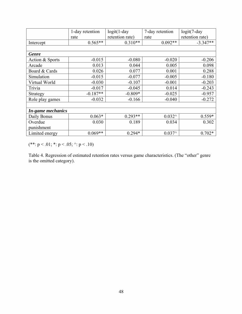
48

1-day retention rate

logit(1-day retention rate)

7-day retention rate

logit(7-day retention rate)

Intercept 0.565** 0.310** 0.092** -3.347**

Genre Action & Sports -0.015 -0.080 -0.020 -0.206Arcade 0.013 0.044 0.005 0.098Board & Cards 0.026 0.077 0.001 0.288Simulation -0.015 -0.077 -0.005 -0.180Virtual World -0.030 -0.107 -0.001 -0.203Trivia -0.017 -0.045 0.014 -0.243Strategy -0.187** -0.809* -0.025 -0.957Role play games -0.032 -0.166 -0.040 -0.272

In-game mechanics Daily Bonus 0.063* 0.293** 0.032^ 0.559*Overdue punishment

0.030 0.189 0.034 0.302

Limited energy 0.069** 0.294* 0.037^ 0.702* (**: p < .01; *: p < .05; ^: p < .10) Table 4. Regression of estimated retention rates versus game characteristics. (The “other” genre is the omitted category).