On the chain rule for the divergence of BV like vector fields

On the chain rule for the divergence of BV like

vector fields: applications, partial results, open

problems

Luigi Ambrosio, Camillo De Lellis, Jan Maly

Scuola Normale Superiore, Piazza dei Cavalieri, 56126 Pisa, ItalyInstitut fur Mathematik, Universitat Zurich, Winterthurerstrasse 190, CH-8057Zurich, SwitzerlandFaculty of Mathematics and Physics, Charles University, Sokolovska 83, 186 75,Praha 8, Czech Republic

1 Introduction

In this paper we study the distributional divergence of vector fields U inRd of the form U = wB, where w is scalar function and B is a weaklydifferentiable vector field (or more in general the divergence of tensor fieldsof the form w ⊗ B). In particular we are interested in a kind of chain ruleproperty, relating the divergence of h(w)B to the divergence of wB. In somesense, if one replaces “divergence” by “derivative” this problem is reminiscentto the problem of writing a chain rule for weakly differentiable functions, atheme that has been investigated in several papers (we mention for instanceVol’pert’s paper [36] and [3] in the BV setting). However, the “divergence”problem seems to be much harder than the “derivative” problem, due to muchstronger cancellation effects. For instance it may happen that U ∈ L∞

loc hasdistributional divergence f ∈ L∞

loc, but f 6= 0 L d-a.e. on U = 0. Thiscannot happen for distributional derivatives, see (16).

The problem of writing a chain rule for vector fields U = wB arises in anatural way when one studies the well-posedness of the PDE D ·(wB) = c, forinstance when B has a space-time structure. Indeed one can use h(s) = s± toestablish uniqueness and comparison principles, very much like in Kruzhkov’stheory of scalar conservation laws (see [29]). When B belongs to a Sobolevspace W 1,p

loc and w ∈ Lqloc, with p, q dual exponents, the chain rule has been

established in [25], obtaining

D · (h(w)B) = (h(w)− wh′(w))D ·B + h′(w)D · (wB), (1)

provided D · (wB) is absolutely continuous with respect to L d. This resulthas been extended in [6] to the case when q = ∞, B ∈ BVloc and both D ·B,D · (wB) are absolutely continuous with respect to L d.

2 Luigi Ambrosio, Camillo De Lellis, Jan Maly

Here we are interested in extending the validity of (1) to the case whenthese divergences are not necessarily absolutely continuous. As we will seethe solution of this problem would have important applications already in thecase when wB is divergence-free, and even in this case we still do not have acomplete solution.

Looking at (1), it is clear that this extension seems to require the existenceof a “good representative” of w, defined not only L d-a.e., but also up to|D ·B|–negligible sets when |D ·B| is not absolutely continuous with respect toL d. Our analysis of this problem takes advantage of the techniques introducedin [6] and of the approximate continuity properties for solutions of transportequations with BV coefficients recently proved in [11].

However, our results are not conclusive and they can be summarized asfollows. First, in Section 3 we prove that D · (h(w)B) is a measure (even in avector-valued setting) and we show a chain rule for the absolutely continuousparts of the divergences

Da · (h(w)B) = (h(w)− wh′(w))Da ·B + h′(w)Da · (wB). (2)

Second, in Section 4 we characterize the jump part Dj · (h(w)B) (i.e. the oneconcentrated on (d−1)-dimensional sets, see Section 2 for a precise definition):

Dj · (h(w)B) =

[

Tr+(B,Σ)h

(

Tr+(wB,Σ)

Tr+(B,Σ)

)

−Tr−(B,Σ)h

(

Tr−(wB,Σ)

Tr−(B,Σ)

)]

Hd−1 Σ, . (3)

Here Σ is any countably rectifiable set on which Dj · B and Dj · (wB) areconcentrated, whereas Tr+(U,Σ) and Tr−(U,Σ) are the normal traces of U onΣ, according to [12], [20], [11]. These one–sided traces coincide for divergence-free vector fields (in general they coincide when the divergence has no jumppart). So, a consequence of (3) is that Dj · (h(w)B) = 0 when both B and wBare divergence-free.

It remains to characterize the remaining part of the divergence, the so-called Cantor part Dc(h(w)B), and it is this part of the problem that has notbeen completely settled by now.

In Section 5 we show a new representation of the commutators (20), seeLemma 2. These commutators play a key role in all proofs of the chain ruleproperty known so far. In Section 6 we use this new representation to showthat

Dc(h(w)B) =

(h(w)− wh′(w))Dc ·B Ω \ Sw + h′(w)Dc · (wB) Ω \ Sw + σ, (4)

where the “error” measure σ is absolutely continuous with respect to |Dc ·B| + |Dc · (wB)| and concentrated on Sw, the L

1–approximate discontinuity

The chain rule for the divergence of vector fields 3

set of w (see Theorem 7 for a more general result). For the definition of theLebesgue limit w(x) we refer to Subsection 2.4.

It remains to understand how large Sw can be. Let us first introduce someterminology.

Definition 1 (Tangential set of B). Let B ∈ BVloc(Ω,Rd), let |DB| denote

the total variation of its distributional derivative and denote by E the Borelset of points x ∈ Ω s.t.

• The following limit exists and is finite:

M(x) := limr↓0

DB(Br(x))

|DB|(Br(x)).

• The Lebesgue limit B(x) exists.

We call tangential set of B the Borel set

E := x ∈ E such that M(x) · B(x) = 0 .

The following result has been proved by a blow-up argument in [11] (seeTheorem 6.5 and (6.8) therein).

Proposition 1. Let B ∈ BVloc(Ω,Rd) and let w ∈ L∞

loc(Ω) be such thatD · (Bw) is a locally finite Radon measure in Ω. Then the inclusion Sw ⊂ Eholds up to |DsB|-negligible sets.

Arguing on the single components of w, the proposition above obviouslyextends to vector-valued functions w. Since the error measure σ in (4) isconcentrated on E and absolutely continuous with respect to |D · B| + |D ·(wB)|, we were thus led to the following question concerning BV vector fields:

(Q) Let B ∈ BVloc ∩ L∞loc(Ω,R

d). Does the Cantor part of the divergence|Dc ·B| vanish on the tangential set?

If this were the case, then the theorems of this paper (see (2), (3), (4))would give a solution to the chain rule problem whenever the measure D ·(wB) is absolutely continuous. Unfortunately the answer to Question (Q) isnegative, as it is proved in Section 8:

Proposition 2. There exists B ∈ BV (R2,R2) such that |Dc · B|(E) > 0,where E denotes the tangential set of B.

Still we can pose the following

Question 1 (Divergence problem). Let B ∈ BVloc ∩ L∞loc(Ω,R

d). Under whichconditions the Cantor part of the divergence |Dc ·B| vanishes on the tangentialset?


The following more concrete version of Question 1 would still give usefulpartial answers to the chain rule problem (see also Remark 1 below):

Question 2. Let B ∈ BVloc ∩ L∞loc(Ω,R

d) and let ρ ∈ L∞(Ω) be such thatρ ≥ C > 0 and D · (ρB) = 0. Is it true that |Dc ·B| vanishes on the tangentialset of B ?

In particular, as we explain in Section 7, an affirmative answer to Question2, combined with some elementary computations and with some remarks of[10], would give an extension of the DiPerna–Lions theory of renormalizedsolutions to transport equations

∂tu+ b · ∇xu = 0

u(0, ·) = u0

when the coefficients b are BV and nearly incompressible. Here by nearlyincompressible we mean that there exists a positive function ρ with log ρ ∈ L∞

satisfying

∂tρ+D · (ρb) = 0 in the sense of distributions on R+t ×Rn . (5)

Then, as remarked in [10], we could use this extension of DiPerna–Lionstheory to prove the following conjecture of Bressan on compactness of ODEs(which indeed was our initial main motivation for investigating the chain rule):

Conjecture 1 (Bressan’s compactness conjecture). Let bn : Rt ×Rdx → Rd be

smooth maps and denote by Φn the solution of the ODEs:

d

dtΦn(t, x) = bn(t, Φn(t, x))

Φn(0, x) = x .

(6)

Assume that the fluxes Φn are nearly incompressible, i.e. that for some con-stant C we have

C−1 ≤ det(∇xΦn(t, x)) ≤ C , (7)

and that ‖bn‖∞ + ‖∇bn‖L1 is uniformly bounded. Then the sequence Φn isstrongly precompact in L1

loc.

We refer to Section 7 for the details.

Remark 1. We close this introduction by pointing out some natural conditionsunder which one could investigate the Divergence Problem:

• B = ∇α ∈ BVloc(Ω) for some α ∈W 1,∞loc (in this case D ·B = ∆α);

• B is a (semi)-monote operator, that is

〈B(y)−B(x), y − x〉 ≥ λ|x− y|2 ∀x, y ∈ Ω . (8)

• B is both curl–free and (semi)-monotone.


2 Main notation and preliminary results

2.1 Decomposition of measures

We denote by L d the Lebesgue measure in Rd and by H k(E) the Hausdorffk-dimensional measure of a set E ⊂ Rd. In the sequel we denote by Ω ageneric open set in Rd. If µ is a nonnegative Borel measure in Ω we say thatµ is concentrated on a Borel set F if µ(Ω \ F ) = 0. For a Borel set F ⊂ Ω,the restriction µ F is defined by

µ F (E) := µ(F ∩ E) for any Borel set E ⊂ Ω.

The same operation can be defined for vector valued measures µ with finitetotal variation in Ω. Unless otherwise stated, weak∗ convergence of measures isunderstood in the duality with continuous and compactly supported functions.

We now recall the following elementary results in Measure Theory (see forinstance Proposition 1.62(b) of [5]):

Proposition 3. Let µh be a sequence of Radon measures on Ω ⊂ Rd, whichconverge weakly∗ to µ and assume that |µh| converge weakly∗ to λ. Then λ ≥|µ| and if E is a compact set such that λ(∂E) = 0, then µh(E) → µ(E).

Proposition 4. Let µ be a Radon measure on Ω. We fix a standard kernel ρ ∈C∞

c (Rd) supported in the unit ball, we take the standard family of mollifiersρδ and on every Ω ⊂⊂ Ω we consider µ ∗ ρδ for δ < dist (Ω, ∂Ω). Thenµ ∗ ρδ converges weakly∗ to µ in Ω and |µ ∗ ρδ| converges weakly∗ to |µ| in Ω.

Let µ be a Radon vector valued measure on Ω. By the Lebesgue decompo-sition theorem, µ has a unique decomposition into absolutely continuous partµa and singular part µs with respect to Lebesgue measure L d. Further, bythe Radon-Nikodym theorem there exists a unique f ∈ L1

loc(Ω,Rk) such that

µa = fL d.One can further decompose µs as follows:

Proposition 5 (Decomposition of the singular part). If |µs| vanisheson any H d−1-negligible set, then µs can be uniquely written as a sum µc+µj

of two measures such that

(a)µc(A) = 0 for every A such that H d−1(A) < +∞;(b) µj = fH d−1 Jµ for some Borel set Jµ σ-finite with respect to H d−1.

The proof of this Proposition is analogous to the proof of decompositionof derivatives of BV functions (and indeed in this case the decompositionscoincide), see Proposition 3.92 of [5]. In this proof, the Borel set Jµ is definedas

Jµ :=

x ∈ Ω

∣

∣

∣

∣

∣

lim supr↓0

|µ|(Br(x))

rd−1> 0

. (9)


These measures will be called, respectively, jump part and Cantor part of themeasure µ.

If µ is given by a distributional divergence D ·U , then µa, µj , and µc willbe denoted respectively by Da · U , Dj · U , and Dc · U .

2.2 Normal traces of divergence–measure fields

In this section we recall some basic facts about the trace properties of vectorfields whose divergence is a measure (see [12], the unpublished work [14], [20],and finally [11]).

Thus, let U ∈ L∞loc(Ω,R

d) be such that its distributional divergence D ·Uis a measure with locally finite variation in Ω. The starting point is to definefor every C1 open set Ω′ ⊂ Ω the distribution Tr(U, ∂Ω′) as

〈Tr(U, ∂Ω′), ϕ〉 :=

∫

Ω′

∇ϕ · U +

∫

Ω′

ϕd [D · U ] ∀ϕ ∈ C∞c (Ω). (10)

It was proved in [12] that there exists a unique g ∈ L∞loc(Ω ∩ ∂Ω′) such that

〈Tr(U, ∂Ω′), ϕ〉 =

∫

∂Ω′

gϕ dH d−1 .

By a slight abuse of notation, we denote the function g by Tr(U, ∂Ω′) as well.Given an oriented C1 hypersurface Σ, we can locally view it as the bound-

ary of an open set Ω1 having νΣ as unit exterior normal. In this way the traceTr+(U,Σ) is well defined, and the trace Tr−(U,Σ) is defined analogously.

In order to extend the notion of trace to countably H d−1-rectifiable sets,defined below, we need a stronger locality property: in [12] it was proved (seealso the recent proof in [11]) that the trace operator is local in a strong sense,i.e. if Ω1, Ω2 ⊂⊂ Ω are two C1 open sets, then

Tr(U, ∂Ω1) = Tr(U, ∂Ω2) H d−1–a.e. on ∂Ω1 ∩ ∂Ω2, (11)

if the exterior unit normals coincide on ∂Ω1 ∩ ∂Ω2.

Definition 2 (Countably H d−1-rectifiable sets). We say that Σ ⊂ Rd

is countably H d−1-rectifiable if there exist (at most) countably many C1 em-bedded hypersurfaces Γi ⊂ Rd such that

Hd−1

(

Σ \⋃

i

Γi

)

= 0.

Using the decomposition of a rectifiable set Σ in pieces of C1 hypersur-faces we can define an orientation of Σ and the normal traces of U on Σ asfollows: by the rectifiability property we can find countably many orientedC1 hypersurfaces Σi and pairwise disjoint Borel sets Ei ⊂ Σi ∩ Σ such that


H d−1 (Σ \ ∪iEi) = 0; then we define νΣ(x) equal to the classical normal toΣi for any x ∈ Ei. Analogously, we define

Tr+(U,Σ) := Tr+(U,Σi), Tr−(U,Σ) := Tr−(U,Σi) H d−1-a.e. on Ei.

The locality property ensures that this definition depends on the orienta-tion νΣ , as in the case of oriented C1 hypersurfaces, but it does not dependon the choice of Σi and Ei, up to H d−1-negligible sets.

We end this subsection by stating two useful propositions, which corre-spond to Propositions 3.4 and 3.6 of [11] (see also [20]).

Proposition 6 (Jump part of D ·U). Let the divergence of C ∈ L∞loc(Ω,R

d)be a measure with locally finite variation in Ω. Then:

(a) |D · U |(E) = 0 for any H d−1-negligible set E ⊂ Ω.(b) If Σ ⊂ Ω is a C1 hypersurface then

D · U Σ = (Tr+(U,Σ)− Tr−(U,Σ))H d−1 Σ. (12)

Thanks to Proposition 6(a) it turns out that for any U ∈ L∞loc(Ω,R

d)whose divergence is a locally finite measure in Ω there exist a Borel functionf and a set J = JD·U such that

Dj · U = fHd−1 JD·U . (13)

Proposition 7 (Fubini’s Theorem for traces). Let U be as above and letF ∈ C1(Ω). Then

Tr(U, ∂F > t) = U · ν H d−1–a.e. on Ω ∩ ∂F > t

for L 1-a.e. t ∈ R, where ν denotes the exterior unit normal to F > t.

Notice that the coarea formula gives that F = t∩ |∇F | = 0 is H d−1-negligible for L 1-a.e. t ∈ R, therefore the theory of traces applies to the setsΣ = F = t for L 1-a.e. t ∈ R.

2.3 BV and BD functions

For B ∈ L1loc(Ω;Rm) we denote by DB = (DiB

l) the derivative in the senseof distributions of B, i.e. the Rm×d-valued distribution defined by

DiBl(ϕ) := −

∫

Ω

Bl ∂ϕ

∂xidx ∀ϕ ∈ C∞

c (Ω), 1 ≤ i ≤ d, 1 ≤ l ≤ m.

In the case when m = d we denote by EB the symmetric part of the distri-butional derivative of B, i.e.,

EB := (EilB), EilB :=1

2(DiB

l +DlBi) 1 ≤ i, l ≤ d.


Definition 3 (BV and BD functions). We say that B ∈ L1(Ω;Rm) hasbounded variation in Ω, and we write B ∈ BV (Ω;Rm), if DB is representableby a Rm×d-valued measure, still denoted with DB, with finite total variationin Ω.We say that B ∈ L1(Ω;Rd) has bounded deformation in Ω, and we writeB ∈ BD(Ω), if EijB is a Radon measure with finite total variation in Ω forany i, j = 1, . . . , d.

It is a well known fact that for B ∈ BV one has DB << H d−1. The sameproperty holds for EB when B ∈ BD (see for instance Remark 3.3 of [4]).Therefore we can apply the decomposition of Subsection 2.1 to the measuresDB and EB and we will use the notation DaB (EaB), DcB (EcB), and DjB(EjB), respectively for the absolutely continuous part, Cantor part, and jumppart of DB (EB). The distributional divergence D ·B :=

∑

iDiBi =

∑

iEiiBis a well defined measure with finite total variation in Ω when B ∈ BD(Ω).

2.4 Fine properties of BV functions

In this subsection we recall the fine properties of Rm-valued BV functionsdefined in an open set Ω ⊂ Rd.

The L1–approximate discontinuity set SB ⊂ Ω of a locally summableB : Ω → Rm and the Lebesgue limit are defined as follows: x /∈ SB if andonly if there exists z ∈ Rm satisfying

limr↓0

r−d

∫

Br(x)

|B(y)− z| dy = 0.

The vector z, if it exists, is unique and denoted by B(x), the Lebesgue limitof B at x. It is easy to check that the set SB is Borel and that B is a Borelfunction in its domain (see §3.6 of [5] for details). By Lebesgue differentiationtheorem the set SB is Lebesgue negligible and B = B L d-a.e. in Ω \ SB .

In a similar way one can define the L1–approximate jump set JB ⊂ SB , byrequiring the existence of a, b ∈ Rm with a 6= b and of a unit vector ν suchthat

limr↓0

r−d

∫

B+r (x,ν)

|B(y)− a| dy = 0, limr↓0

r−d

∫

B−

r (x,ν)

|B(y)− b| dy = 0,

whereB+

r (x, ν) := y ∈ Br(x) : 〈y − x, ν〉 > 0 ,

B−r (x, ν) := y ∈ Br(x) : 〈y − x, ν〉 < 0 .

(14)

The triplet (a, b, ν), if exists, is unique up to a permutation of a and b and achange of sign of ν, and denoted by (B+(x), B−(x), ν(x)), where B±(x) arecalled Lebesgue one-sided limits of B at x. It is easy to check that the set


JB is Borel and that B± and ν can be chosen to be Borel functions in theirdomain (see again §3.6 of [5] for details).

Denoting by η ⊗ ξ the linear map from Rd to Rm defined by v 7→ η〈ξ, v〉,the following structure theorem holds (see for instance Theorem 3.77 andProposition 3.92 of [5]):

Proposition 8 (BV structure theorem). If B ∈ BVloc(Ω,Rm), then

H d−1(SB \ JB) = 0 and JB is a countably H d−1–rectifiable set. Moreover

DjB = (B+ −B−)⊗ νH d−1 JB , (15)

|DaB|(u−1(N)) + |DcB|(u−1(N)) = 0for any L 1-negligible Borel set N ⊂ R.

(16)

As a corollary, since DaB and DcB are both concentrated on Ω \ SB , weconclude that |DaB| + |DcB|–a.e. x is a Lebesgue point for B, with valueB(x). The space of functions of special bounded variation (denoted by SBV )is defined as follows:

Definition 4 (SBV ). Let Ω ⊂ Rd be an open set. The space SBV (Ω,Rm)is the set of all u ∈ BV (Ω,Rm) such that Dcu = 0.

2.5 Fine properties of BD functions

As in the case of BV functions, also for BD functions B the set JB is countablyH d−1–rectifiable (see [4]). Though the question whether H d−1(SB \JB) = 0is still open, in [4] it was proved that:

Proposition 9. If B ∈ BD(Ω), then

EjB = (B+ −B−)⊙ νHd−1 JB ,

where 2a⊙ b := a⊗ b+ b⊗ a.

Similarly, we can define:

Definition 5 (SBD). SBD(Ω) is the set of all B ∈ BD(Ω) such that EcB =0.

2.6 Vol’pert chain rule and Alberti’s rank one Theorem

We end this section by recalling the classical chain–rule formula for BV func-tions of Vol’pert (see [36] and Theorem 3.96 of [5]) and a deep result of Alberticoncerning the structure of DsB (see [1]).

Theorem 1 (Vol’pert chain rule). Let v ∈ BVloc(Ω,Rm) and let Φ ∈

C1(Rm,Rh) be a map with a bounded gradient. Then Φ v ∈ BVloc(Ω,Rh)

and the measure D(Φ v) can be explicitly computed as

D(Φ v) = ∇Φ(v) ·Dav +∇Φ(v) ·Dcv +(

Φ(v+)− Φ(v−))⊗ νHd−1 Jv .


Theorem 2 (Alberti’s rank one theorem). Let B ∈ BVloc(Ω,Rm). Then

there exist Borel functions ξ : Ω → Sd−1, η : Ω → Sm−1 such that

DsB = η ⊗ ξ|DsB| . (17)

3 Chain rule: The absolutely continuous part

In this and in the next three sections we will study the problem of computingthe divergence D · (h(w)B) when B is a BV function and w is an L∞ functionsuch that D · (wB) is a measure.

To simplify the statements, in this and in the next two sections we willalways assume that the divergence of wB is a measure with locally finite totalvariation.

Remark 2. Note that, when U ∈ L∞(Rd,Rd) and D · U is a measure withlocally finite total variation, one has the estimate

|D · U(Br(x))| ≤ αd−1‖U‖∞rd−1 ,

where αd−1 denotes the d − 1–dimensional volume of the unit sphere. Bystandard arguments, this implies that |D · U |(E) = 0 for every Borel set Esuch that H d−1(E) = 0.

Therefore we can decompose D ·U into its absolutely continuous, Cantor,and jump part, which will be denoted respectively by Da · U , Dc · U , andDj · U .

Definition 6 (BV measures). We say that a positive locally finite measureσ in Ω is a BV measure if there exists an at most countable Borel partitionΩll∈I of Ω and functions fl ∈ BVloc(Ω) such that σ Ωl ≪ |Dfl| for anyl ∈ I.

Notice that it is not restrictive to assume that the functions fl are boundedand nonnegative, by a truncation argument. Also, it is immediate to checkusing the uniqueness of decomposition in Cantor and jump part that σ Ωl ≪|Dfl| implies σj Ωl ≪ |Djfl| and σ

c Ωl ≪ |Dcfl|. As a consequence, since|Djf | is concentrated on a countably H d−1-rectifiable set for any f ∈ BVloc(precisely the L1–approximate jump set of f), the same is true for the jumppart σj of a BV measure σ.

Theorem 3 (Absolutely continuous part). Let B ∈ BDloc(Ω), w ∈L∞loc(Ω;Rk), and h ∈ C1(Rk), and assume that D · (wB) is a measure with

locally finite total variation. Then

(a)D · (h(w)B) is a measure with locally finite variation in Ω and

Da · (h(w)B) =[

h(w)−

k∑

i=1

wi∂h

∂zi(w)

]

Da ·B +

k∑

i=1

∂h

∂zi(w)Da · (wiB) . (18)


(b) If B ∈ BVloc, then for any open set A ⊂⊂ Ω we have

|Ds · (h(w)B)| A ≤ L1|Ds ·B|+ L2|D

s · (wB)| , (19)

where the constants L1 and L2 depend only on L := ‖w‖L∞(A) and‖h‖C1(BL(0)).

(c) If B ∈ BVloc and D · (wiB) are BV measures, then |D · (h(w)B)| is a BVmeasure as well.

Before going into the proof of the previous theorem, we need some defini-tions and preliminary lemmas. First of all, ρδ will denote a standard familyof mollifiers in Rd, that is ρ ∈ C∞

c (B1(0)) is even with ρ ≥ 0,∫

ρ = 1 andρδ(x) = δ−dρ

(

xδ

)

. We set

I(ρ) :=

∫

Rd

|z||∇ρ(z)| dz .

Moreover, we define the commutators

Tδ := (D · (Bw)) ∗ ρδ −D · (B(w ∗ ρδ)) , (20)

and we denote by T iδ the component (D · (Bwi)) ∗ ρδ −D · (B(wi ∗ ρδ)). The

next Proposition is Theorem 2.6 of [11].

Proposition 10 (BD commutators estimate). Let B ∈ BDloc(Ω) and letw ∈ L∞

loc(Ω). Let ρ be a radial convolution kernel. Then:

(a)The distributions defined by (20) are induced by measures with locally uni-formly bounded variation in Ω as δ ↓ 0.

(b) Any weak∗ limit σ of a subsequence of |Tδ|δ↓0 as δ ↓ 0 is a singularmeasure which satisfies the bound

σ A ≤ ‖w‖L∞(A)

(

d+ I(ρ))

|EsB| for any open set A ⊂⊂ Ω. (21)

In the case where B ∈ BVloc we can consider more general convolutionkernels and give more refined estimates. In this we follow [6] and define, forevery convolution kernel ρ and any d× d matrix M , the quantity:

Λ(M,ρ) :=

∫

Rd

∣

∣〈M · z,∇ρ(z)〉∣

∣ dz . (22)

In the following proposition we write the matrix valued measure DsB asM |DsB|, where M : Ω → Rd×d is a Borel function with |M | = 1 |DsB|-a.e.in Ω.

Proposition 11 (BV commutators estimate). Let B ∈ BVloc(Ω;Rd) andlet ρ be an even convolution kernel. Then, any measure σ which is the weak∗

limit in Ω of a subsequence of |Tδ| satisfies the estimate

σ A ≤ ‖w‖L∞(A) [Λ(M(·), ρ)|DsB|+ |Ds ·B|] (23)

for all open sets A ⊂⊂ Ω.


This proposition is the analog of Theorem 3.2 of [6], with the only differ-ence that the commutators considered here in (20) are more general than thoseconsidered in [6]. Indeed the commutators considered in [6] can be written onlyunder the assumption that the divergence of B is absolutely continuous. InAppendix A we show the minor modifications needed to adapt the proof ofTheorem 3.2 of [6].

The final ingredient for the proof of Theorem 3 is the following elementarylemma

Lemma 1. Let

K :=

ρ ∈ C∞c (B1(0)) such that ρ ≥ 0 is even, and

∫

B1(0)ρ = 1

. (24)

If D ⊂ K is dense with respect to the strong W 1,1 topology, then for everyξ, η ∈ Rd we have

infρ∈D

Λ(η ⊗ ξ, ρ) = |〈ξ, η〉| =∣

∣tr (η ⊗ ξ)∣

∣ . (25)

The proof of this lemma is equal to the the proof of Lemma 3.3 of [6] (seealso Remark 3.8(1) in the same paper), but since the statement of Lemma 3.3of [6] is slightly weaker, for the reader’s convenience we include the proof ofLemma 1 in Appendix B. We now come to

Proof (of Theorem 3). (a) Let us fix a radial convolution kernel ρ and defineTδ as in (20). Then, we compute

D · (h(w ∗ ρδ)B)

=∑

i

∂h

∂zi(w ∗ ρδ)∇(wi ∗ ρδ) ·B + h(w ∗ ρδ)D ·B

=∑

i

∂h

∂zi(w ∗ ρδ)D · [(wi ∗ ρδ)B]

+

[

h(w ∗ ρδ)−∑

i

(wi ∗ ρδ)∂h

∂zi(w ∗ ρδ)

]

D ·B

=∑

i

∂h

∂zi(w ∗ ρδ)[(D · (Bwi)) ∗ ρδ]−

∑

i

∂h

∂zi(w ∗ ρδ)T

iδ (26)

+

[

h(w ∗ ρδ)−∑

i

(wi ∗ ρδ)∂h

∂zi(w ∗ ρδ)

]

D ·B . (27)

As δ ↓ 0, D · (h(w ∗ ρδ)B) converges to D · (h(w)B) in the distribution sense.On any open set A ⊂⊂ Ω the measures [(D ·(Bw))∗ρδ] enjoy uniform boundson their total variations. In view of Proposition 10, the same holds for Tδ.Since w ∈ L∞

loc we conclude easily that the sum of (26) and (27) converges,up to subsequences, to a Radon measure µ = D · (h(w)B) on Ω.


Define Sδ := ∂h∂zi

(w ∗ ρδ)Tiδ . Note that |Sδ| ≤ C|T i

δ |, where C locallydepends only on ‖w‖∞ and h. Hence from Proposition 10 we conclude thatany weak limit of a subsequence of |Sδ| is singular and from Proposition 3 weconclude that any limit point of Sδ as δ ↓ 0 is a singular measure.

We use the decomposition [(D · (Bw)) ∗ ρδ] = [(Da · (Bw)) ∗ ρδ] + [(Ds ·(Bw)) ∗ ρδ]. By Proposition 3 again, the measures

µδ2 :=

∑

i

∂h

∂zi(w ∗ ρδ)[(D

s · (Bwi)) ∗ ρδ]

converge (up to subsequences) to singular measures. Moreover, if we writeDa · (Bw) = fL d, we get that [(Da · (Bw))∗ρδ] = f ∗ρδL

d. Since ∂h∂zi

(w ∗ρδ)

converges to ∂h∂zi

(w) pointwise almost everywhere and f ∗ ρδ converges to f

strongly in L1loc, we conclude that

µδ1 :=

∑

i

∂h

∂zi(w ∗ ρδ)[(D

a · (Bwi)) ∗ ρδ]

converges to

[

∑

i

∂h

∂zi(w)fi

]

Ld =

∑

i

∂h

∂zi(w)Da · (Bwi) .

In a similar way we can treat the last term in (27) and we conclude thatthe sum of the expressions (26) and (27) converges (up to subsequences) toµ = µ1 + µ2, where

• µ2 is singular with respect to L d and is the limit of

µδ2 +

∑

i

∂h

∂zi(w ∗ ρδ)T

iδ +

[

h(w ∗ ρδ)−∑

i

(wi ∗ ρδ)∂h

∂zi(w ∗ ρδ)

]

Ds ·B ;

• µ1 is absolutely continuous and

µ1 = limδ↓0

µδ1 +

[

h(w ∗ ρδ)−∑

i

(wi ∗ ρδ)∂h

∂zi(w ∗ ρδ)

]

Da ·B

=

[

h(w)−

k∑

i=1

wi∂h

∂zi(w)

]

Da ·B +

k∑

i=1

∂h

∂zi(w)Da · (wiB) .

From this we easily get (18).

(b) From the argument of the previous step, we conclude that Ds ·(h(w)B)is the limit (in the sense of distributions) of the sums of the following expres-sions:


∑

i

∂h

∂zi(w ∗ ρδ)

[

(Ds · (Bwi)) ∗ ρδ]

+

[

h(w ∗ ρδ)−∑

i

(wi ∗ ρδ)∂h

∂zi(w ∗ ρδ)

]

Ds ·B

, (28)

∑

i

∂h

∂zi(w ∗ ρδ)T

iδ . (29)

Clearly, any limit point of the sum in (28) is a measure which is bounded onany open set A ⊂⊂ Ω by

L1|Ds · (Bw)|+ L2|D

s ·B| ,

where L1 and L2 only depend on L := ‖w‖L∞(A) and ‖h‖C1(BL(0)).Now, fix an open set A ⊂⊂ Ω and let ν be any limit point of (29). Ac-

cording to Proposition 11 we have

|ν| A ≤ ‖w‖L∞(A)Λ(M(·), ρ)|DsB|+ ‖w‖L∞(A)|Ds ·B|

Thus, choosing subsequences for which both terms in (28) and (29) are con-verging, we find

|Ds · (h(w)B))| A ≤ L1|Ds · (Bw)|+L2|D

s ·B|+L3Λ(M(·), ρ)|DsB| (30)

for some constants Li independent of Q and of ρ and depending only on A.Now, let τ be the positive part of the measure |Ds(h(w)B)| − L1|D

s · (Bw)|and let g be its Radon–Nikodym derivative with respect to |DsB|. Then from(30) it follows that, for any even convolution kernel ρ, the inequality

g(x) ≤ L2|tr(M(x))|+ L3Λ(M(x), ρ)

holds for |DsB|–a.e. x ∈ A. Let D be a countable set of mollifiers which isdense in the W 1,1 strong topology in the set K of (24). Then,

g(x) ≤ L2

∣

∣tr (M(x))∣

∣+ L3 infρ∈D

Λ(M(x), ρ) for |DsB|–a.e. x ∈ A.

Recall Alberti’s Theorem:M(x) = η(x)⊗ξ(x). Thus, from Lemma 1 it followsthat

g(x) ≤ L2

∣

∣tr (M(x))∣

∣+ L3

∣

∣tr (M(x))∣

∣ ,

so that τ A ≤ (L2 + L3)|Ds ·B|. Hence, setting L4 = L2 + L3, we conclude

that

|Ds · (h(w)B))| ≤ L1|Ds · (Bw)|+ L4|tr(M)||DsB|

= L1|Ds · (Bw)|+ L4|D

s ·B| . (31)

(c) It is an immediate consequence of (19). ⊓⊔


4 Chain rule: The jump part

In this section we prove the following

Theorem 4 (Jump part). Let h ∈ C1(Rk), B ∈ BDloc and let Σ ⊂ Ω beany oriented countably H d−1-rectifiable set. Then

D · (h(w)B) Σ =

[

Tr+(B,Σ)h

(

Tr+(wB,Σ)

Tr+(B,Σ)

)

−Tr−(B,Σ)h

(

Tr−(wB,Σ)

Tr−(B,Σ)

)]

Hd−1 Σ,

where the ratio Tr+(wB,Σ)Tr+(B,Σ)

(resp. Tr−(wB,Σ)Tr−(B,Σ)

) is arbitrarily defined at points

where the trace Tr+(B,Σ) (resp. Tr−(B,Σ)) vanishes.Moreover, if Dj · (wiB) are concentrated on a countably H d−1-rectifiable

set Σ, then Dj(h(w)B) is concentrated on Σ.

The key for proving Theorem 4 is the following theorem. The scalar caseis proved in [11]. In the vector-valued case the proof is analogous, but we givea detailed one for the reader’s convenience.

Theorem 5 (Change of variables for traces). Let Ω′ ⊂⊂ Ω be an opendomain with a C1 boundary and let h ∈ C1(Rk). Then

Tr(h(w)B, ∂Ω′) = h

(

Tr(wB, ∂Ω′)

Tr(B, ∂Ω′)

)

Tr(B, ∂Ω′) H d−1-a.e. on ∂Ω′.

Proof. It is not restrictive to assume that the larger open set Ω is boundedand it has a C1 boundary.Step 1. Let Ω′′ = Ω \Ω′. In this step we prove that

Tr(h(w)B, ∂Ω′′) = h

(

Tr(wB, ∂Ω′′)

Tr(B, ∂Ω′′)

)

Tr(B, ∂Ω′′) H d−1-a.e. on ∂Ω′′,

under the assumption that the components of B and w are bounded andbelong to the Sobolev space W 1,1(Ω′′). Indeed, the identity is trivial if bothw and B are continuous up to the boundary, and the proof of the generalcase can be immediately achieved by a density argument based on the strongcontinuity of the trace operator fromW 1,1(Ω′′) to L1(∂Ω′′,H d−1 ∂Ω′′) (seefor instance Theorem 3.88 of [5]).Step 2. In this step we prove the general case. Let us apply Gagliardo’stheorem on the surjectivity of the trace operator from W 1,1 into L1 to obtaina bounded vector field B1 ∈W 1,1(Ω′′;Rd) whose trace on ∂Ω′ ⊂ ∂Ω′′ is equalto the trace of B, seen as a function in BD(Ω′). In particular Tr(B, ∂Ω′) =−Tr(B1, ∂Ω

′′). Defining


B(x) :=

B(x) if x ∈ Ω′

B1(x) if x ∈ Ω′′,

it turns out that B ∈ BDloc(Ω) and that

|EB|(∂Ω′) = 0. (32)

Let us consider the function θ := Tr(wB, ∂Ω′)/Tr(B, ∂Ω′) (set equal to 0wherever the denominator is 0) and let us prove that ‖θ‖L∞(∂Ω′) is less than‖w‖L∞(Ω′). Indeed, writing ∂Ω

′ as the 0-level set of a C1 function F with|∇F | > 0 on ∂Ω′ and F = t ⊂ Ω′ for t > 0 sufficiently small, by Proposi-tion 7 we have

−‖w‖L∞(Ω′)Tr(B, ∂F > t) ≤ Tr(wB, ∂F > t)

≤ ‖w‖L∞(Ω′)Tr(B, ∂F > t)

H d−1-a.e. on F = t for L 1-a.e. t > 0 sufficiently small. Passing to thelimit as t ↓ 0 and using the w∗-continuity of the trace operator (see [20], [11])we recover the same inequality on F = 0, proving the boundedness of θ.

Now, still using Gagliardo’s theorem, we can find a bounded function w1 ∈W 1,1(Ω′′;Rk) whose trace on ∂Ω′ is given by θ, so that the normal trace ofw1iB1 on ∂Ω′′ is equal to Tr(wiB, ∂Ω

′) on the whole of ∂Ω′. Defining

w(x) :=

w(x) if x ∈ Ω′

w1(x) if x ∈ Ω′′,

by Proposition 6 we obtain

|D · (wiB)|(∂Ω′) = 0 i = 1, . . . , k. (33)

Let us apply now (19) in Theorem 3 and (32), (33), to obtain that thedivergence of the vector field h(w)B is a measure with finite total variation inΩ, whose restriction to ∂Ω′ vanishes. As a consequence, Proposition 6 gives

Tr+(h(w)B, ∂Ω′) = Tr−(h(w)B, ∂Ω′) H d−1-a.e. on ∂Ω′. (34)

By applying (34), Step 1, and finally our choice of B1 and w1 the followingchain of equalities holds H d−1-a.e. on ∂Ω′:

Tr(h(w)B, ∂Ω′) = Tr+(h(w)B, ∂Ω′) = Tr−(h(w)B, ∂Ω′)

= Tr(h(w1)B1, ∂Ω′′) = h

(

Tr(w1B1, ∂Ω′′)

Tr(B1, ∂Ω′′)

)

Tr(B1, ∂Ω′′)

= h

(

Tr(wB, ∂Ω′)

Tr(B, ∂Ω′)

)

Tr(B, ∂Ω′).

⊓⊔

Proof (of Theorem 4). If Σ is a compact set contained in a C1 hypersurface∂Ω′ the statement is a direct consequence of Proposition 6 and of Theorem 5.The general case follows by the rectifiability of Σ, recalling the way in whichtraces on rectifiable sets have been defined. Finally, the last statement is adirect consequence of (19). ⊓⊔


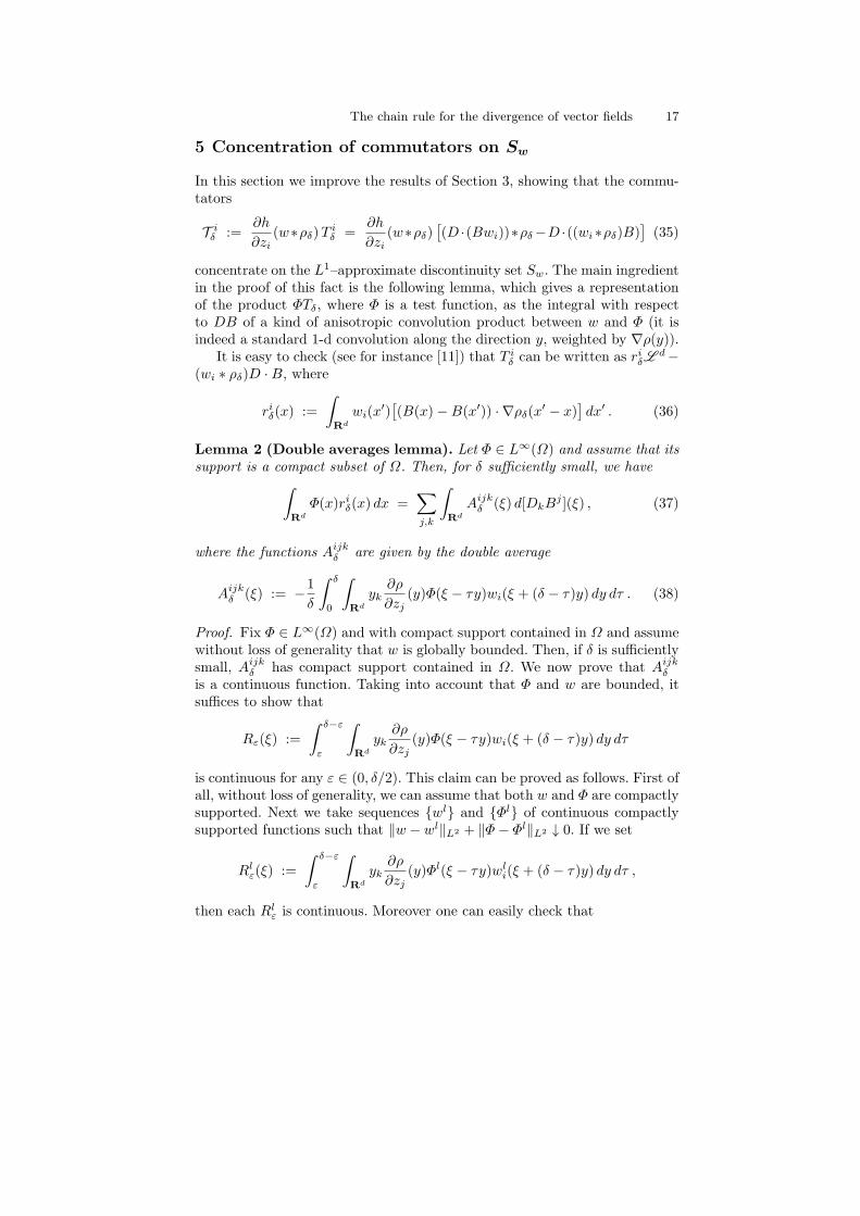
5 Concentration of commutators on Sw

In this section we improve the results of Section 3, showing that the commu-tators

T iδ :=

∂h

∂zi(w∗ρδ)T

iδ =

∂h

∂zi(w∗ρδ)

[

(D ·(Bwi))∗ρδ−D ·((wi ∗ρδ)B)]

(35)

concentrate on the L1–approximate discontinuity set Sw. The main ingredientin the proof of this fact is the following lemma, which gives a representationof the product ΦTδ, where Φ is a test function, as the integral with respectto DB of a kind of anisotropic convolution product between w and Φ (it isindeed a standard 1-d convolution along the direction y, weighted by ∇ρ(y)).

It is easy to check (see for instance [11]) that T iδ can be written as riδL

d−(wi ∗ ρδ)D ·B, where

riδ(x) :=

∫

Rd

wi(x′)[

(B(x)−B(x′)) · ∇ρδ(x′ − x)

]

dx′ . (36)

Lemma 2 (Double averages lemma). Let Φ ∈ L∞(Ω) and assume that itssupport is a compact subset of Ω. Then, for δ sufficiently small, we have

∫

Rd

Φ(x)riδ(x) dx =∑

j,k

∫

Rd

Aijkδ (ξ) d[DkB

j ](ξ) , (37)

where the functions Aijkδ are given by the double average

Aijkδ (ξ) := −

1

δ

∫ δ

0

∫

Rd

yk∂ρ

∂zj(y)Φ(ξ − τy)wi(ξ + (δ − τ)y) dy dτ . (38)

Proof. Fix Φ ∈ L∞(Ω) and with compact support contained in Ω and assumewithout loss of generality that w is globally bounded. Then, if δ is sufficientlysmall, Aijk

δ has compact support contained in Ω. We now prove that Aijkδ

is a continuous function. Taking into account that Φ and w are bounded, itsuffices to show that

Rε(ξ) :=

∫ δ−ε

ε

∫

Rd

yk∂ρ

∂zj(y)Φ(ξ − τy)wi(ξ + (δ − τ)y) dy dτ

is continuous for any ε ∈ (0, δ/2). This claim can be proved as follows. First ofall, without loss of generality, we can assume that both w and Φ are compactlysupported. Next we take sequences wl and Φl of continuous compactlysupported functions such that ‖w − wl‖L2 + ‖Φ− Φl‖L2 ↓ 0. If we set

Rlε(ξ) :=

∫ δ−ε

ε

∫

Rd

yk∂ρ

∂zj(y)Φl(ξ − τy)wl

i(ξ + (δ − τ)y) dy dτ ,

then each Rlε is continuous. Moreover one can easily check that


|Rlε(ξ)−Rε(ξ)| ≤ Cδε−n

(

‖Φ‖L2‖w − wl‖L2 + ‖wl‖L2‖Φl − Φ‖L2

)

.

Therefore Rlε → Rε uniformly, and we conclude that Rε is continuous.

Now, fix B and δ as in the statement of the lemma. We approximate Bin L1

loc with a sequence of smooth functions Bn, in such a way that DkBjn

converge weakly∗ to DkBj on Ω. Hence, we have that

Rin(x) :=

∫

Rd

wi(x′)[

(Bn(x)−Bn(x′)) · ∇ρδ(x

′ − x)]

dx′

converge strongly in L1loc to riδ. Moreover, since Aijk

δ is a continuous andcompactly supported function, we have

limn→∞

∫

Aijkδ (ξ)d[DkB

jn](ξ) =

∫

Aijkδ (ξ)d[DkB

j ](ξ) .

Hence it is enough to prove the statement of the lemma for Bn, which aresmooth functions.

Thus, we fix a smooth function B and compute

−

∫

riδ(x)Φ(x) dx

= −

∫

Rd

Φ(x)

∫

Rd

wi(x′)[

(B(x)−B(x′)) · ∇ρδ(x′ − x)

]

dx′ dx

= −

∫

Rd×Rd

Φ(x)wi(x+ δy)B(x)−B(x+ δy)

δ· ∇ρ(y) dy dx

=

∫

Rd×Rd

Φ(x)wi(x+ δy)1

δ

∫ δ

0

∑

k,j

yk∂Bj

∂zk(x+ τy)

∂ρ

∂zj(y) dτ dy dx

=∑

k,j

∫

Rd

[

1

δ

∫ δ

0

∫

Rd

yk∂ρ

∂zj(y)Φ(ξ − τy)wi(ξ + (δ − τ)y) dy dτ

]

∂Bj

∂zk(ξ) dξ .

Since the measure ∂Bj

∂zkL d is equal to DkB

j , the claim of the lemma follows.⊓⊔

Theorem 6 (Concentration of commutators on Sw). Assume that B ∈BVloc(Ω;Rd) and w ∈ L∞

loc(Ω;Rk). Then any limit point as δ ↓ 0 of T iδ is a

measure concentrated on Sw.

Proof. We rewrite T iδ as

T iδ =

∂h

∂zi(w ∗ ρδ) r

iδ L

d −∂h

∂zi(w ∗ ρδ) (wi ∗ ρδ)D ·B . (39)

We define the matrix–valued measures


α := DB (Ω \ Sw)

β := DB Sw

and the measures

γ := [D ·B] (Ω \ Sw)

λ := [D ·B] Sw .

Then we introduce the measures Siδ and Ri

δ given by the following linearfunctionals on ϕ ∈ Cc(Ω):

〈Siδ, ϕ〉 :=

∑

j,k

∫

Rd

gijkδ (ξ) d[αkj ](ξ)

−

∫

Rd

ϕ(x)∂h

∂zi(w ∗ ρδ(x))wi ∗ ρδ(x) dγ(x) (40)

〈Riδ, ϕ〉 :=

∑

j,k

∫

Rd

gijkδ (ξ) d[βkj ](ξ)

−

∫

Rd

ϕ(x)∂h

∂zi(w ∗ ρδ(x))wi ∗ ρδ(x) dλ(x) , (41)

where

gijkδ (ξ) := −1

δ

∫ δ

0

∫

Rd

yk∂ρ

∂zj(y)ϕ(ξ − τy)

·∂h

∂zi(w ∗ ρδ(ξ − τy))wi(ξ + (δ − τ)y) dy dτ . (42)

This formula for gijkδ comes from the formulas for Aijkδ of Lemma 2, where we

choose as Φ the function

Φ := ϕ∂h

∂zi(w ∗ ρδ) .

Hence, comparing (42) with (39) and (38), from Lemma 2 we conclude thatT iδ = Si

δ +Riδ.

Let Ri0 be any weak limit of a subsequence Ri

δnδn↓0 and let Si

0 be any

weak limit of a subsequence (not relabeled) of Siδn. In what follows we will

prove that

(i) Ri0 ≪ |λ|+ |β|

(ii)Si0 = 0.

Since |λ| and |β| are concentrated on Sw, (i) and (ii) prove the Theorem.

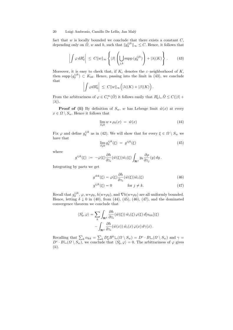
Proof of (i) Let us fix an open set Ω ⊂⊂ Ω and a smooth function ϕ

with |ϕ| ≤ 1 and with support K ⊂ Ω. If we define gijkδ as in (42), from the


fact that w is locally bounded we conclude that there exists a constant C,depending only on Ω, w and h, such that ‖gijkδ ‖∞ ≤ C. Hence, it follows that

∣

∣

∣

∣

∫

ϕdRiδ

∣

∣

∣

∣

≤ C‖w‖∞

|β|

⋃

j,k

supp (gijkδ )

+ |λ|(K)

. (43)

Moreover, it is easy to check that, if Kε denotes the ε–neighborhood of K,then supp (gijkδ ) ⊂ K2δ. Hence, passing into the limit in (43), we concludethat

∣

∣

∣

∣

∫

ϕdRi0

∣

∣

∣

∣

≤ C‖w‖∞

(

|λ|(K) + |β|(K))

.

From the arbitrariness of ϕ ∈ C∞c (Ω) it follows easily that Ri

0 Ω ≤ C(|β|+|λ|).

Proof of (ii) By definition of Sw, w has Lebesge limit w(x) at everyx ∈ Ω \ Sw. Hence it follows that

limδ↓0

w ∗ ρδ(x) = w(x) (44)

Fix ϕ and define gijkδ as in (42). We will show that for every ξ ∈ Ω \ Sw wehave that

limδ↓0

gijkδ (ξ) = gijk(ξ) (45)

where

gijk(ξ) := −ϕ(ξ)∂h

∂zi(w(ξ))wi(ξ)

∫

Rd

yk∂ρ

∂zj(y) dy .

Integrating by parts we get

gikk(ξ) = ϕ(ξ)∂h

∂zi(w(ξ))wi(ξ) (46)

gijk(ξ) = 0 for j 6= k. (47)

Recall that gijkδ , ϕ, w∗ρδ, h(w∗ρδ), and ∇h(w∗ρδ) are all uniformly bounded.Hence, letting δ ↓ 0 in (40), from (44), (45), (46), (47), and the dominatedconvergence theorem we conclude that

〈Si0, ϕ〉 =

∑

k

∫

Rd

∂h

∂zi(w(ξ)) wi(ξ)ϕ(ξ) d[αkk](ξ)

−

∫

Rd

∂h

∂zi(w(x)) wi(x)ϕ(x) dγ(x) .

Recalling that∑

k αkk =∑

kDckB

k (Ω \ Sw) = Dc · B (Ω \ Sw) and γ =Dc · B (Ω \ Sw), we conclude that 〈Si

0, ϕ〉 = 0. The arbitrariness of ϕ gives(ii).


Hence, to finish the proof, it suffices to show (45). Recalling the smoothnessof ϕ and the fact that ρ is supported in the ball B1(0) we conclude that itsuffices to show that

Iδ :=1

δ

∫ δ

0

∫

B1(0)

∣

∣

∣

∣

∂h

∂zj(w ∗ ρδ(ξ − τy))wi(ξ + (δ − τ)y)

−∂h

∂zj(w(ξ)) wi(ξ)

∣

∣

∣

∣

dy dτ (48)

converges to 0. Then, we write

Iδ ≤1

δ

∫ δ

0

∫

B1(0)

∣

∣

∣

∣

∂h

∂zj(w ∗ ρδ(ξ − τy))−

∂h

∂zj(w(ξ))

∣

∣

∣

∣

|wi(ξ + (δ − τ)y)| dy dτ

+1

δ

∫ δ

0

∫

B1(0)

∣

∣

∣

∣

∂h

∂zj(w(ξ))

∣

∣

∣

∣

∣

∣wi(ξ + (δ − τ)y)− wi(ξ)∣

∣ dy dτ

≤C1

δ

∫ δ

0

∫

B1(0)

∣

∣w ∗ ρδ(ξ − τy)− w(ξ)∣

∣ dy dτ

+C2

δ

∫ δ

0

∫

B1(0)

∣

∣w(ξ + (δ − τ)y)− w(ξ)∣

∣ dξ dτ

=: C1J1δ + C2J

2δ

where the constants C1 and C2 depend only on ξ, w, and h. Note that

J1δ =

1

δ

∫ δ

0

∫

B1(0)

∣

∣w(ξ + τy)− w(ξ)∣

∣ dy dτ

=1

δ

∫ δ

0

[

1

τd

∫

Bτ (ξ)

∣

∣w(z)− w(ξ)∣

∣ dz

]

dτ ,

and

J2δ =

1

δ

∫ δ

0

∫

B1(0)

∣

∣w ∗ ρδ(ξ + τy)− w(ξ)∣

∣ dy dτ

=1

δ

∫ δ

0

[

1

τd

∫

Bτ (ξ)

∣

∣w ∗ ρδ(z)− w(ξ)∣

∣ dz

]

dτ .

Hence, since w(ξ) is the Lebesgue limit of w at ξ, we conclude that J1δ+J

2δ → 0.

This completes the proof. ⊓⊔

6 Chain rule: The Cantor part

The following theorem provides together with Theorem 3 and Theorem 5 afull chain rule for the distributional divergence out of Sw.


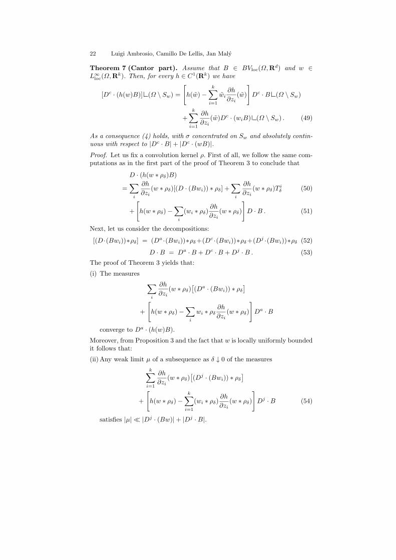
Theorem 7 (Cantor part). Assume that B ∈ BVloc(Ω,Rd) and w ∈

L∞loc(Ω,R

k). Then, for every h ∈ C1(Rk) we have

[Dc · (h(w)B)] (Ω \ Sw) =

[

h(w)−

k∑

i=1

wi∂h

∂zi(w)

]

Dc ·B (Ω \ Sw)

+

k∑

i=1

∂h

∂zi(w)Dc · (wiB) (Ω \ Sw) . (49)

As a consequence (4) holds, with σ concentrated on Sw and absolutely contin-uous with respect to |Dc ·B|+ |Dc · (wB)|.

Proof. Let us fix a convolution kernel ρ. First of all, we follow the same com-putations as in the first part of the proof of Theorem 3 to conclude that

D · (h(w ∗ ρδ)B)

=∑

i

∂h

∂zi(w ∗ ρδ)[(D · (Bwi)) ∗ ρδ] +

∑

i

∂h

∂zi(w ∗ ρδ)T

iδ (50)

+

[

h(w ∗ ρδ)−∑

i

(wi ∗ ρδ)∂h

∂zi(w ∗ ρδ)

]

D ·B . (51)

Next, let us consider the decompositions:

[(D ·(Bwi))∗ρδ] = (Da ·(Bwi))∗ρδ+(Dc ·(Bwi))∗ρδ+(Dj ·(Bwi))∗ρδ (52)

D ·B = Da ·B +Dc ·B +Dj ·B . (53)

The proof of Theorem 3 yields that:

(i) The measures

∑

i

∂h

∂zi(w ∗ ρδ)

[

(Da · (Bwi)) ∗ ρδ]

+

[

h(w ∗ ρδ)−∑

i

wi ∗ ρδ∂h

∂zi(w ∗ ρδ)

]

Da ·B

converge to Da · (h(w)B).

Moreover, from Proposition 3 and the fact that w is locally uniformly boundedit follows that:

(ii) Any weak limit µ of a subsequence as δ ↓ 0 of the measures

k∑

i=1

∂h

∂zi(w ∗ ρδ)

[

(Dj · (Bwi)) ∗ ρδ]

+

[

h(w ∗ ρδ)−k∑

i=1

(wi ∗ ρδ)∂h

∂zi(w ∗ ρδ)

]

Dj ·B (54)

satisfies |µ| ≪ |Dj · (Bw)|+ |Dj ·B|.


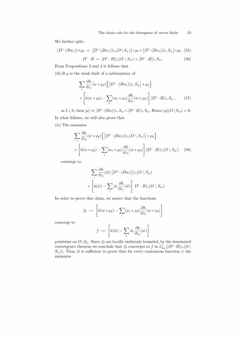
We further split:

(Dc ·(Bwi))∗ρδ =[

Dc ·(Bwi)) (Ω\Sw)]

∗ρδ+[

Dc ·(Bwi)) Sw

]

∗ρδ (55)

Dc ·B = [Dc ·B] (Ω \ Sw) + [Dc ·B] Sw . (56)

From Propositions 3 and 4 it follows that

(iii) If µ is the weak limit of a subsequence of

∑

i

∂h

∂zi(w ∗ ρδ)

[

Dc · (Bwi)) Sw

]

∗ ρδ

+

[

h(w ∗ ρδ)−∑

i

(wi ∗ ρδ)∂h

∂zi(w ∗ ρδ)

]

[Dc ·B] Sw , (57)

as δ ↓ 0, then |µ| ≪ |Dc ·(Bw)| Sw+ |Dc ·B| Sw. Hence |µ|(Ω\Sw) = 0.

In what follows, we will also prove that

(iv) The measures

∑

i

∂h

∂zi(w ∗ ρδ)

[

Dc · (Bwi)) (Ω \ Sw)]

∗ ρδ

+

[

h(w ∗ ρδ)−∑

i

(wi ∗ ρδ)∂h

∂zi(w ∗ ρδ)

]

[Dc ·B] (Ω \ Sw) . (58)

converge to

∑

i

∂h

∂zi(w)

[

Dc · (Bwi)]

(Ω \ Sw)

+

[

h(w)−∑

i

wi∂h

∂zi(w)

]

Dc ·B (Ω \ Sw) .

In order to prove this claim, we notice that the functions

fδ :=

[

h(w ∗ ρδ)−∑

i

(wi ∗ ρδ)∂h

∂zi(w ∗ ρδ)

]

converge to

f :=

[

h(w)−∑

i

wi∂h

∂zi(w)

]

pointwise on Ω\Sw. Since fδ are locally uniformly bounded, by the dominatedconvergence theorem we conclude that fδ converges to f in L1

loc(|Dc ·B| (Ω \

Sw)). Thus, it is sufficient to prove that for every continuous function ψ themeasures


νδ := ψ(w ∗ ρδ)

[

(Dc · (Bwi)) (Ω \ Sw)]

∗ ρδ

converge toψ(w)

[

Dc · (Bwi)]

(Ω \ Sw) . (59)

Let us denote by ν the measure[

Dc ·(Bwi)]

(Ω\Sw) and by fδ the functionsψ(w ∗ ρδ). Then, if ϕ ∈ C∞

c (Ω) is any test function, we have∫

ϕfδd(ν ∗ ρδ) =

∫

(ϕfδ) ∗ ρδdν =

∫

Ω\Sw

(ϕfδ) ∗ ρδd[Dc · (Bwi)] .

We claim that

limδ↓0

[

(ϕfδ) ∗ ρδ]

(x) = limδ↓0

[

(ϕψ(w ∗ ρδ)) ∗ ρδ]

(x) = ϕ(x)ψ(w(x))

for any x ∈ Ω \ Sw. Indeed, since ϕ and f are regular and w is uniformlybounded on a neighborhood of the support of ϕ, we can write

oscδ := supy∈Bδ(x)

|ϕ(y)fδ(y)− ϕ(x)ψ(w(x))|

≤ C1δ + C2 supy∈Bδ(x)

|w ∗ ρδ(y)− w(x)|

= C1δ + C2 supy∈Bδ(x)

1

δd

∣

∣

∣

∣

∣

∫

Bδ(y)

[

w(z)− w(x)]

ρ

(

z − y

δ

)

dz

∣

∣

∣

∣

∣

≤ C1δ +C3

δd

∫

B2δ(x)

|w(z)− w(x)| dz . (60)

Since w has Lebesgue limit w(x) at x, it follows that the right hand side of(60) tends to 0 as δ ↓ 0. Thus, we can conclude

limδ↓0

∣

∣

∣

[

(ϕfδ) ∗ ρδ]

(x)− ϕ(x)ψ(w(x))∣

∣

∣

= limδ↓0

1

δn

∣

∣

∣

∣

∣

∫

Bδ(x)

(ϕ(y)fδ(y)− ϕ(x)ψ(w(x)))ρ

(

y − x

δ

)

dy

∣

∣

∣

∣

∣

≤ C limδ↓0

oscδ = 0 .

The pointwise convergence of [(ϕfδ) ∗ ρδ](x) just proved gives

limδ↓0

∫

Ω\Sw

(ϕfδ) ∗ ρδd[Dc · (Bwi)] =

∫

Ω\Sw

ϕψ(w)d[Dc · (Bwi)] .

This implies that the measures νδ converge weakly to (59), concluding theproof of claim (iv).

(v) Any limit point of the measures

∑

i

∂h

∂zi(w ∗ ρδ)T

iδ


is concentrated on Sw. This is precisely the statement of Proposition 6.The proof can now achieved noticing that the decompositions above yield

that D ·(h(w)B) is the sum of absolutely continuous measures (the one consid-ered in item (i)), jump measures (the ones considered in item (ii)), measuresconcentrated on Sw (the ones considered in items (iii) and (v)) and finallythe measures in item (iv). Restricting the divergence to the L d-negligibleset Sw, the Cantor part of all these contributions, with the exception ofthe one considered in (iv), disappear. Finally, we obtain (4) from (49) withσ := Dc · (h(w)B) Sw, and Theorem 3 gives that this measure is absolutelycontinuous with respect to |Dc ·B|+ |Dc · (wB)|. ⊓⊔

7 Bressan’s compactness conjecture and its variants

In the following section we use the theorems proved so far to study transportequations and Bressan’s compactness conjecture. In Subsection 7.1 we showthat the results of the previous sections provide a DiPerna–Lions theory fornearly incompressible BV fields which satisfy a certain technical assumption.In Subsection 7.2 we show how this implies certain cases of Conjecture 1.In both sections we also explain why a positive answer to Question 2 wouldremove the technical assumption, giving a DiPerna–Lions theory for all nearlyincompressible BV fields and a full positive answer to Conjecture 1. Finallyin Section 7.3 we remark that Theorem 3 and Theorem 4 yields a DiPerna–Lions theory for nearly incompressible SBD fields, and hence allows to provea variant of Conjecture 1.

7.1 DiPerna–Lions theory and continuity equation for nearlyincompressible fields

We first introduce the following notion

Definition 7 (Near incompressibility). A vector field b ∈ L∞(Rt ×Rn

x ,Rnx) is called nearly incompressible if there exists a positive function ρ

with log ρ ∈ L∞ such that

∂tρ+Dx · (ρb) = 0 in the sense of distributions on R+t ×Rn . (61)

Next we introduce a concept of weak solution for transport equations withnearly incompressible BV coefficients. The problem in defining a solution of(62) under the assumptions above is that the distribution b · ∇xw cannot bedefined as div (bw)−wdiv b, since w is an L∞ function, defined up to sets of 0Lebesgue measure, and div b can have nontrivial singular part. This problemis overcome by using the existence of the function ρ in the definition of nearincompressibility.


Definition 8 (Weak solutions). Fix a nearly incompressible vector field b ∈L∞ ∩ BV (or b ∈ L∞ ∩ BD) and a function ρ as in Definition 7. For anyc ∈ L∞ we say that u ∈ L∞ is a ρ–weak solution of

∂tu+ b · ∇xu = cL d

u(0, ·) = u0

(62)

if u solves the following Cauchy problem

∂t(ρu) +Dx · (bρu) = ρcL d

u(0, ·) = u0

(63)

in the following (distributional) sense:∫

R+×Rn

ρ(t, x)

u(t, x)[

∂tϕ(t, x) + b(t, x) · ∇xϕ(t, x)]

+ c(t, x)ϕ(t, x)

dx dt

= −

∫

Rn

ρ(0, x)u0(x)ϕ(0, x) dx (64)

for every test function ϕ ∈ C∞(R ×Rn).

Remark 3. The attainment of initial conditions as in (64) is justified by thefollowing remarks. Set B = (1, b). From (61) we get that D · (ρB) = 0. Weorient the hyperplane I := t = 0 ⊂ Rt × Rn

x with the vector (1, 0, . . . , 0).Thus, the vector field ρB has a well defined normal trace Tr+(ρB, I). Sincethe normal trace Tr+(B, I) is identically equal to 1, the trace of ρ on I canbe uniquely defined as ρ(0, ·) := Tr+(ρB, I).

Then, in this subsection we will prove:

Theorem 8 (Uniqueness of weak solutions). Let b ∈ BVloc ∩ L∞(R+ ×

Rn,Rn) be nearly incompressible. Consider B := (1, b) and assume that Dc ·Bvanishes on its tangential set E. Then:

(a) If ρ and ζ satisfy (61), then any ρ–weak solution of (62) is a ζ–weaksolution.

(b) If u is a ρ–weak solution of (62) and γ is a C1 function, then γ(u) is aρ–weak solution of the Cauchy problem (62) with initial data γ(u0) andright hand side γ′(u)cL d;

(c) For any u0 ∈ L∞ there exists a unique ρ–weak solution of (62).

Thus it makes sense to call the function u of Definition 8 the weak solutionof (62).

Remark 4. Clearly, a positive answer to Question 2 would give that the as-sumption |Dc · B|(E) = 0 satisfied by any nearly incompressible b. HenceTheorem 8 would give a DiPerna–Lions theory for every nearly incompress-ible BVloc ∩ L

∞ field.


The proof of Theorem 8 is based on the following “renormalization”lemma:

Lemma 3 (Renormalization Lemma). Let Ω ⊂ Rd be open, B ∈ BVloc ∩L∞(Ω,Rd), ρ ∈ L∞(Ω) and u, s ∈ L∞(Ω,Rl). Assume that

D · (ρB) = 0 and ρ ≥ C > 0 (65)

D · (ρuiB) = siLd for i = 1, . . . , l. (66)

Then, if E denotes the tangential set of B, we have

D · (ρβ(u)B)−l∑

i=1

∂β

∂yi(u)siL

d ≪ |Dc ·B| E ∀β ∈ C1(Rl) . (67)

Proof. Set k := l + 1 and define w ∈ L∞(Ω,Rk) as w1 = ρ, wi = ρui−1 fori = 2, . . . , l. Moreover define H : Rk → R as

H(z1, . . . , zk) = z1 β

(

z2z1, . . . ,

zkz1

)

. (68)

Clearly, H is C1 on the set Rk \ z1 = 0. Define m := max‖ρ‖∞, ‖w‖∞and let h ∈ C1(Rk) be such that h = H on the set

D :=

z1 ≥C

2and |z| ≤ m+ 1

. (69)

Then we have D · (w1B) = 0, D · (wiBi) = si for i = 2, . . . , k, and D ·(ρβ(u)B) = D · (h(w)B).

Absolutely continuous part. We use formula (18) and we compute

Da · (h(w)B) :=

[

h(w)−

k∑

i=1

∂h

∂zi(w)wi

]

Da ·B +

k∑

i=2

∂h

∂zi(w)si .

Note that h is a 1–homogeneous function on D. Thus

h(z)−k∑

i=1

∂h

∂zi(z)zi = 0 for every z ∈ D.

Since the essential range of w is contained in D, we get that

h(w)−

k∑

i=1

∂h

∂ziwi = 0 L d-almost everywhere ,

k∑

i=2

∂h

∂zi(w)si =

l∑

i=1

∂β

∂yi(u)si L d-almost everywhere.


Thus we conclude that

Dc · (h(w)B) =l∑

i=1

∂β

∂yi(u)siL

d . (70)

Cantor part According to (49) we have

[

Dc · (h(w)B)]

(Ω \ E) =

[

h(w)−

k∑

i=1

∂h

∂zi(w)wi

]

Dc ·B (Ω \ E) ,

where w(x) is the Lebesgue limit of w at x, which on Ω \E exists |Dc ·B|–a.e..From the very definition of Lebesgue limit, it follows that whenever it exists,it belongs to the closure of the essential range of w, that is still contained inD. Hence, arguing as above, we conclude that

[

Dc · (h(w)B)]

(Ω \ E) = 0 . (71)

Jump part Let JB be the jump set, let ν be an orienting unit normal toJB , and let B+ and B− be respectively the right and left traces. Then it followsfrom Theorem 4 that there exist Borel functions w+ and w−, characterizedas quotients of traces of wB and B, such that

Dj · (h(w)B) =[

h(w+)B+ · ν − h(w−)B− · ν]

Hd−1 JB . (72)

If we define the functions hi : Rk → R as

hi(z1, . . . , zk) = zi

we can apply the same theorem in order to get

Dj · (hi(w)B) =[

w+i B

+ · ν − w−i B

− · ν]

Hd−1 JB . (73)

But since D · (hi(w)B) = D · (wiB) = 0, we conclude that

w+i B

+ · ν = w−i B

− · ν H d−1–a.e. on JB . (74)

We fix x ∈ JB such that w+i (x)B

+(x) · ν(x) = w−i (x)B

− · ν(x) and we distin-guish two cases:

Case 1 B+(x) · ν(x) 6= 0 6= B−(x) · ν(x).Then w+(x) and w−(x) are the right and left Lebesgue limits of w at x.

This means that they both belong to the essential range of w and hence to D.To simplify the notation in the following formulas we drop the (x) dependence.

The formulas (74) give that

w+i = w−

i

[

B− · ν

B+ · ν

]

.


Recall that D ⊂ z1 6= 0 and hence we conclude

w+i

w+1

=w−

i

w−1

for i = 1, . . . , k. (75)

Since h = H on D, plugging (75) into (68) and using (74) we conclude

h(w+)B+ · ν − h(w−)B− · ν

= w+1 β

(

w+2

w+1

, . . . ,w+

k

w+1

)

B+ · ν − w−1 β

(

w−2

w−1

, . . . ,w−

k

w−1

)

B− · ν

= β

(

w+2

w+1

, . . . ,w+

k

w+1

)

[

w+1 B

+ · ν − w−1 B

− · ν]

= 0 .

Case 2 Remaining cases.If both B+(x) · ν(x), B−(x) · ν(x) vanish, then clearly

h(w+(x))B+(x) · ν(x)− h(w−(x))B−(x) · ν(x) = 0 .

Assume that one of them vanishes but the other not. Without loosing ourgenerality we assume that B+(x) · ν(x) = 0 6= B−(x) · ν(x). Then, w−(x) isin D. This means that w−

1 (x) 6= 0. But then we would have

w+1 (x)B

+(x) · ν(x) = 0 6= w−1 (x)B

−(x) · ν(x) ,

which contradicts (74).

From the analysis of these two cases we conclude that

Dj · (h(w)B) = 0 . (76)

Conclusion From (70), (71), and (76) we conclude that

D · (h(w)B) = Dc · (h(w)B) (Ω \ E) . (77)

From (19) we know that

Ds · (h(w)B) ≪ |Ds ·B| . (78)

Thus, (77) and (78) give (67). ⊓⊔

Proof (of Theorem 8). (a) Assume that u is a ρ–weak solution and that ζ isanother weak solution of (61). Let u1 := u, u2 := ζ/ρ, B = (1, b), s1 = cρ ands2 = 0. Apply the renormalization Lemma 3 to β(u1, u2) = u1u2 to concludethat

∂t(β(u1, u2)ρ) +Dx · (bβ(u1, u2)ρ)

=

(

s1∂β

∂y1(u1, u2) + s2

∂β

∂y2(u1, u2)

)

Ld+1 .


Note that s2 = 0 and that βy1(u1, u2) = u2, hence

∂t(uζ) +Dx · (uζ) = cζL d+1 . (79)

This means that u and ζ solve (79) in the sense of distributions in R+ ×Rn.To take care of the initial condition in the sense of Remark 3, it is sufficientto apply Theorem 5.

(b) Applying Lemma 3 we conclude that ∂t(ργ(u)) + Dx · (bργ(u)) =ρcγ′(u)L d in the sense of distributions in R+ × Rn. As above, we applyTheorem 5 in order to take care of the initial condition in the sense of Remark3.

(c) Let u1 and u2 be two ρ–solutions of the same Cauchy problem. Defineu := u1 − u2 and note that u solves in the sense of distributions the Cauchyproblem

∂t(uρ) +Dx · (uρb) = 0

u(0, ·) = 0 .

From (b) we conclude that u2 solves the same Cauchy problem. This meansthat for every ϕ ∈ C∞

c (R ×Rn) we have

∫

R+×Rn

ρ(t, x)u2(t, x)[

∂tϕ(t, x) + b(t, x) · ∇xϕ(t, x)]

dx dt = 0 .

Thus, we can apply Lemma 2.11 of [10] to conclude that u2 ≡ 0. ⊓⊔

7.2 Some cases of Conjecture 1

We now apply the results of the previous section to prove the following:

Proposition 12 (Partial answer to Bressan’s Conjecture). Let bn be asin Conjecture 1 and assume that bn → b strongly in L1

loc. If Dc · B vanishes

on the tangential set of B, then the conclusion of Conjecture 1 holds and thefluxes Φn have a unique limit.

Remark 5. If Question 2 has a positive answer, then any limiting B satisfiesthe assumption of Proposition 12, and therefore Conjecture 1 would have afull positive answer.

Proof. The arguments are the same as those given in Section 4 of [10] and theyconsist in a standard modification of the usual arguments used in DiPerna–Lions theory of renormalized solutions to pass from a uniqueness theoremon transport equations to compactness properties of solutions to ordinarydifferential equations (see [25] and also [6], [7] for a different approach).

Since (Φn) is locally uniformly bounded it suffices to prove, thanks to thedominated convergence theorem, that for every T ∈ R there exists a function


Φ(T, ·) ∈ L1loc(R

d,Rd) such that Φn(T, ·) converge strongly to Φ(T, ·) in L1loc.

We will prove this property for T < 0, the case T > 0 being analogous.

Step 1. For each t denote by Ψn(t, ·) the inverse of Φn(t, ·). Let us considerthe ODE

d

dtΛn(t, x) = bn(t, Λn(t, x))

Λn(T, x) = x ,

and note thatΛn(t, x) = Φn(t, Ψn(T, x)) . (80)

Thus, if we denote by Jn(t, ·) the Jacobian of Λn(t, ·), we get that C−2 ≤Jn(t, ·) ≤ C2. Denote by Γn(t, ·) the inverse of Λn(t, ·) and set

ρn(t, x) :=1

Jn(t, Γn(t, x)).

Since, by the area formula, ρn(t, ·) is the density of the of the image of L d

by the flow map Λn(t, ·), the maps ρn solve the continuity equation

∂tρn + divx (bnρn) = 0

ρn(T, ·) = 1(81)

in the sense of distributions.Any weak∗ limit point ρ of a subsequence of (ρn) will still solve

∂tρ+ divx (bρ) = 0

ρ(T, ·) = 1(82)

in the sense of distributions. If ζ is any other distributional solution of (82),then w := ζ/ρ is a weak solution (in the sense of Definition 8, up to a timeshift) of

∂tw + b · ∇xw = 0

w(T, ·) = 1 .(83)

Therefore from Theorem 8 (again up to a time shift) we conclude w = 1, thatis ζ = ρ. Therefore we conclude that the whole sequence (ρn) converges to ρ.

Step 2. Now fix w ∈ L∞(Rd) and set wn(t, x) := w(Γn(t, x)). These functionsare weak solutions to the transport equations

∂twn + bn · ∇xwn = 0

wn(T, ·) = w(·) .(84)


Passing to a subsequence we can assume that ρn(k)wn(k) converge to a functionv weakly∗ in L∞. If we define w := v/ρ, then w is the unique weak solution of

∂tw + b · ∇xw = 0

w(T, ·) = w(·) .(85)

Therefore the whole sequence (ρnwn) converges to ρw. From Theorem 8(b) itfollows that, for every β ∈ C1, the functions wn := β(wn) and w := β(w) arethe unique weak solutions of

∂twn + bn · ∇xwn = 0

wn(T, ·) = β(

w(·))

,

∂tw + b · ∇xw = 0

w(T, ·) = β(

w(·))

.(86)

Therefore arguing as above we conclude that

ρnβ(wn) weak∗-converge in L∞ to ρβ(w) for every β ∈ C1. (87)

Step 3. For every given smooth function ϕ ∈ Cc(R+ ×Rd) we write

∫

ϕρn(wn − w)2 =

∫

ϕρnw2n − 2

∫

ρnwnw +

∫

ρnw2 .

Then, from (87) with β(s) = s2 we get:

limn→∞

∫

ϕρnw2n =

∫

ϕρw2 ,

limn→∞

∫

ϕρnwnw =

∫

ϕρw2 ,

limn→∞

∫

ϕρnw2 =

∫

ϕρw2 ,

hence

limn→∞

∫

ϕρn(wn − w)2 = 0 .

Since ρn ≥ C−2 > 0 and ϕ is arbitrary, we conclude that (wn) convergesto w strongly in L2

loc. Since wn(t, x) = w(Γn(t, x)) we conclude that forevery w ∈ L∞(Rd) the functions w(Γn(t, x)) converge strongly in L1

loc to aunique function. Therefore we conclude that Γn converge strongly in L1

loc toa function Γ on [T, 0]×Rd.

Step 4. Fix R > 0 and note that for each x the curves Γn(·, x) have a uni-formly bounded Lipschitz constant, and so possibly modifying Γ in a L d+1-negligible set we can assume that the same is true for Γ . Since the mean valuetheorem provides us an infinitesimal sequence (ǫn) ⊂ (T, 0) such that


limn→∞

∫

BR

|Γn(ǫn, x)− Γ (ǫn, x)| dx = 0

we obtain as a consequence that Γn(0, ·) → Γ (0, ·) strongly in L1(BR). Re-calling the identity (80) we have Λn(0, x) = Ψn(T, x). Therefore Γn(0, ·) is theinverse of Ψn(T, ·), which means Γn(0, ·) = Φn(T, ·). This allows us to con-clude that Φn(T, ·) converge strongly in L1(BR) to Γ (0, ·) =: Φ(T, ·). Since Ris arbitrary the proof of the convergence of (Φn) is achieved. ⊓⊔

7.3 SBD–variant of Conjecture 1

The following are corollaries of Theorem 3 and Theorem 4:

Theorem 9 (Uniqueness of weak solutions for SBD coefficients). Letb ∈ SBDloc(R

+ ×Rn,Rn) be nearly incompressible. Then:

(a) If ρ and ζ satisfy (I), then any ρ–weak solution of (62) is a ζ–weak solution;(b) If u is a ρ–weak solution of (62) and γ is a C1 function, then γ(u) is a

ρ–weak solution of the Cauchy problem (62) with initial data γ(u0) andwith right hand side γ′(u)cL d;

(c) For any u0 ∈ L∞ there exists a unique ρ–weak solution of (62).

Thus it makes sense to call the u of Definition 8 the weak solution of (62).

Proposition 13 (SBD variant of Bressan’s compactness conjecture).Let bn be a sequence of smooth maps bn : Rt ×Rd

x → Rdx, uniformly bounded.

Let Φn be as in (6) and assume that they satisfy condition (7). If bn → b andb ∈ SBDloc, then Φn has a unique strong limit in L1

loc.

Since the proof are essentially analogous to the proofs of Theorem 8 andProposition 12 we do not give the details here.

8 Proof of Proposition 2

We set Ω :=

(x, y) ∈ R2 : 1 < x < 2 , 0 < y < x

. We construct a scalarfunction u ∈ L∞ ∩BV (Ω) with the following properties:

(a)Dcyu 6= 0;

(b)Dxu + Dy(u2/2) is a pure jump measure, i.e. it is concentrated on the

jump set Ju.

Given such a function u, the field B = (1, u)1Ω meets the requirements of theproposition. Indeed, let B = (1, u)1Ω be the precise representative of B. Dueto (b) the Cantor part of Dxu + Dy(u

2/2) vanishes. Hence using the chainrule of Vol’pert we get

Dcxu+ uDc

yu = 0 . (88)


Denote by M(x) the Radon–Nikodym derivative DB/|DB|. Then we have

M · B|DcB| = DcB · B

=

(

0 0Dc

xu Dcyu

)

·

(

1u

)

=

(

0Dc

xu+ uDcyu

)

=

(

00

)

.

Hence we conclude that M(x) · B(x) = 0 for |DcB|–a.e. x, that is |DcB| isconcentrated on the tangential set E of B. Therefore |Dc · B|(Ω \ E) = 0.On the other hand, from (a) we have Dc · B = Dc

yu 6= 0. Hence we conclude|Dc ·B|(E) > 0.

We now come to the construction of the desired u. This is achieved as thelimit of a suitable sequence of functions uk.

Step 1. Construction of uk.Consider the auxiliary 1-periodic function σ : R → R defined by

σ(p+ x) = 1− x , 0 < x ≤ 1 , p ∈ Z .

We let γk : [0, 1] → [0, 1] be the usual piecewise linear approximation of theCantor ternary function, that is γ0(z) = z and, for k ≥ 1,

γk(z) =

12γk−1(3z), 0 < z ≤ 1

3 ,

12 ,

13 < z ≤ 2

3 ,

12

(

1 + γk−1(3z − 2))

, 23 < z ≤ 1 .

Notice that

γ′k(z) ∈

0,(3

2

)k(89)

and

|γk(z)− γk−1(z)| ≤1

3· 2−k . (90)

We set G :=]1, 2[×]0, 1[ and we define ϕk : G→ R by

ϕk(x, z) = xz +

k∑

j=1

41−jσ(4j−1x)(

γj−1(z)− γj(z))

.

Note that ϕk is bounded. To describe more precisely the behavior of thisfunction we introduce the following sets: The strips

Ski :=

]

1 + (i− 1)41−k, 1 + i41−k[

× R i = 1, . . . , 4k−1,

and the vertical lines

V ki := i41−k × R i = 1, . . . , 4k−1 − 1 .


Then ϕk is Lipschitz on each rectangle Ski ∩G and it has jump discontinuities

on the segments V ki ∩ G. Therefore ϕk is a BV function and satisfies the

identities Dxϕk = Djxϕk +Da

xϕk and Dyϕk = Dayϕk. Moreover, denoting by

(∂xϕk, ∂yϕk) the density of the absolutely continuous part of the derivative,we get

∂xϕk(x, z) = z + (γ1(z)− z) + (γ2(z)− γ1(z)) + · · ·+ (γk(z)− γk−1(z))

= γk(z) . (91)

Clearly0 ≤ 41−jσ(4j−1x)− 4−jσ(4jx) ≤ 3 · 4−j .

Therefore, using also (89), on each rectangle Ski ∩G we can estimate

∂zϕk(x, z) = x+ σ(x)−(

σ(x)−4−1σ(4x))

γ′1(z)

−(

4−1σ(4x)−4−2σ(42x))

γ′2(z) − · · ·

−(

42−kσ(4k−1x)−41−kσ(4k−1x))

γ′k−1(z)

− 41−kσ(4k−1x) γ′k(z)

≥ 2− 3(

4−1γ′1(z) + · · ·+ 41−kγ′k(z))

− 41−kγ′k(z)

≥ 2− 3

(

3

8+ · · ·+

(

3

8

)k−1)

− 4

(

3

8

)k

.

Since

4

(

3

8

)k

≤ 3

(

(

3

8

)k

+

(

3

8

)k+1

+ · · ·

)

,

we obtain

∂zϕk ≥ 2− 3

(

3

8+

(

3

8

)2

+ · · ·

)

=1

5. (92)

Hence, since ϕk(x, ·) maps [0, 1] onto [0, x], the function

Φk(x, y) := (x, ϕk(x, y))

maps each rectangle Ski ∩G onto Sk

i ∩Ω, and it is bi-Lipschitz on each suchrectangle. This allows to define uk by the implicit equation

uk(

x, ϕk(x, z))

= γk(z) , (93)

and to conclude that 0 ≤ uk ≤ 1 and that uk is Lipschitz on each Ski ∩ Ω.

Therefore uk ∈ L∞ ∩BV (Ω), Dxuk = Daxuk +Dj

xuk and Dyuk = Dayuk.

Step 2. BV bounds.We prove in this step that |Duk|(Ω) is uniformly bounded. This claim and

the bound ‖uk‖∞ ≤ 1 allow to apply the BV compactness theorem to get asubsequence which converges to a bounded BV function u, strongly in Lp for


every p < ∞. In Steps 3 and 4 we will then complete the proof by showingthat u satisfies both the requirements (a) and (b).

By differentiating (93) and using (91) we get the following identity forL 2–a.e. (x, z) ∈ Sk

i ∩G:

0 =∂uk(x, ϕk(x, z))

∂x+∂uk(x, ϕk(x, z))

∂y

∂ϕk(x, z)

∂x

=∂uk(x, ϕk(x, z))


∂yγk(x)

=∂uk(x, ϕk(x, z))


∂yuk(x, ϕk(x, z)).

Since Φk is bi-Lipschitz we get

∂xuk(x, y) + uk∂yuk(x, y) = 0 for L 2–a.e. (x, y) ∈ Ski ∩Ω . (94)

If 4k−1x /∈ N the function uk(x, ·) is non decreasing. Therefore

|Dyuk|(Ω) = Dyuk(Ω) =

∫ 2

1

(

uk(x, x)− uk(x, 0))

dx = 1 . (95)

From (94) we get|Da

xuk|(Ω) ≤ |Dayuk|(Ω) = 1 . (96)

Therefore it remains to bound |Djxuk|(Ω). This consists of

|Djxuk|(Ω) =

4k−1−1∑

i=1

∫

V ki

|u+k − u−k | dH1. (97)

For each x of type 1 + i41−k we compute∫

V ki

|u+k − u−k | dH1 =

∫ x

0

|uk(x+, y)− uk(x

−, y)| dy

=

∫ 1

0

|y : uk(x−, y) < t < uk(x

+, y)| dt

+

∫ 1

0

|y : uk(x+, y) < t < uk(x

−, y)| dt

=

∫ 1

0

|y : uk(x−, y) < γk(z) < uk(x

+, y)| γ′k(z) dz

+

∫ 1

0

|y : uk(x+, y) < γk(z) < uk(x

−, y)| γ′k(z) dz

=

∫ 1

0

|ϕk(x+, z)− ϕk(x

−, z)| γ′k(z) dz

≤ supz∈]0,1[

|ϕk(x+, z)− ϕk(x

−, z)|


(90)

≤4

3

k∑

j=1

8−j(

σ(4j−1x+)− σ(4j−1x−))

. (98)

Combining (97) and (98) we get

|Djxuk|(Ω) ≤

4

3

4k−1−1∑

i=1

k∑

j=1

8−j(

σ(4j−141−ki+)− σ(4j−141−ki−))

=4

3

k∑

j=1

8−j4k−1−1∑

i=1

(

σ(4j−ki+)− σ(4j−ki−))

=4

3

k∑

j=1

8−j4j−1 ≤1

3. (99)

Step 3. Proof of (a).We now fix a bounded BV function u and a subsequence of uk, not re-

labeled, which converges to u strongly in L1. We claim that (a) holds. Moreprecisely we will show that:

(Cl)For L 1–a.e. x the function u(x, ·) is a nonconstant BV function of onevariable which has no absolutely continuous part and no jump part.

(Cl) gives (a) by the slicing theory of BV functions, see Theorem 3.108 of [5].In order to prove (Cl) we proceed as follows. By possibly extracting another

subsequence we assume that uk converges to u L 2–a.e. in Ω. We then show(Cl) for every x such that:

• 4kx 6∈ N for every k;• uk(x, y) converges to u(x, y) for L 1–a.e. y.

Clearly L 1–a.e. x meets these requirements.Fix any such x. Note that x is never on the boundary of any strip Sk

i .Therefore we can denote by gxk the inverse of ϕk(x, ·) and we can use (93) towrite

uk(x, y) = γk(gxk(y)) . (100)

Thanks to (92), the Lipschitz constant of gk is uniformly bounded. Therefore,after possibly extracting a subsequence, we can assume that gk uniformlyconverge to a Lipschitz function g. Since γk uniformly converge to the Cantorternary function γ, we can pass into the limit in (100) to conclude

u(x, y) = γ(g(y)) . (101)

Therefore u(x, ·) is continuous, nondecreasing, nonconstant, and locally con-stant outside a closed set of zero Lebesgue measure (g−1(C), where C is theCantor set). This proves (Cl).


Step 4. Proof of (b).Let u be as in Step 3. From the construction of uk it follows that

Dxuk +Dy(u2k/2) = Dj

xuk . (102)

After possibly extracting a subsequence we can assume that Djxuk converges

weakly∗ to a measure µ. This gives

Dxu+Dy(u2/2) = µ . (103)

Therefore it suffices to prove that µ is concentrated on a set of σ–finite 1–dimensional Hausdorff measure. Indeed µ is concentrated on the union of thecountable family of segments V kk,i. In order to prove this claim it sufficesto show the following tightness property: for every ε > 0 there exists N ∈ Nsuch that

|Djxuk|

⋃

l≥N

4l−1−1⋃

i=1

V li

≤ ε for every k. (104)

Note that

|Djxuk|

⋃

l≥N

4l−1−1⋃

i=1

V li

≤∑

l≥N

4l−1−1∑

i=1

∫

V li

|u+k − u+k | .

Then the same computations leading to (98) and (99) give

|Djxuk|

⋃

l≥N

4l−1−1⋃

j=1

V lj

≤4

3

k∑

l=N

8−l4l−1 ≤1

3 · 2N−1. (105)

This concludes the proof. ⊓⊔

Remark 6. The function u constructed in Proposition 2 solves Burgers’ equa-tion with a measure source

Dtu+Dx(u2/2) = µ , (106)

and has nonvanishing Cantor part. On the other hand in [9] it has been provedthat entropy solutions to Burgers’ equation without source are SBV , i.e. theCantor part of their derivative is trivial. It would be interesting to understandwhether this gain of regularity is due to the entropy condition, or instead BVdistributional solutions of (106) with µ = 0 are always SBV .

A Proof of Proposition 11

In order to prove Proposition 11 we need the following Theorem on the de-composition of difference quotients of BV functions, which is part of Theorem2.4 of [6] (we refer to [6] for the proof). In what follows, for B ∈ BVloc, wedenote by ∇B the L1

loc (matrix valued) function such that DaB = ∇BL d

and by divB the L1loc function such that Da ·B = divBL d.


Theorem 10 (Difference quotients). Let B ∈ BVloc(Rd,Rm) and let z ∈

Rd. Then the difference quotients

B(x+ δz)−B(x)

δ

can be canonically written as B1δ (z)(x) +B2

δ (z)(x), where

(a)B1δ (z) converges strongly in L1

loc to z · ∇B as δ ↓ 0.(b) For any compact set K ⊂ Rd we have

lim supδ↓0

∫

K

∣

∣B2δ (z)(x)

∣

∣ dx ≤ |z||DsB|(K) . (107)

(c) For every compact set K ⊂ Rd we have

supδ∈]0,ε[

∫

K

∣

∣B1δ (z)(x)

∣

∣+∣

∣B2δ (z)(x)

∣

∣ dx ≤ |DB|(Kε) (108)

where Kε := x : dist (x,K) ≤ ε.

Proof (of Theorem 11). As in (36) we write

Tδ := rδLd − (w ∗ ρδ)D ·B,

where

rδ(x) :=

∫

Rd

w(y)[

(B(x)−B(y)) · ∇ρδ(y − x)]

dy

= −

∫

Rd

w(x+ δy)

[

B(x+ δy)−B(x)

δ· ∇ρ(y)

]

dy .

Recalling the notation Da ·B = divBL d, we get

|Tδ| :=∣

∣rδ − (w ∗ ρδ)divB∣

∣Ld + |w ∗ ρδ||D

s ·B| .

Next, using Theorem 10 we write rδ as r1δ + r2δ , where

r1δ(x) :=

∫

Rd

w(x+ δy)B1δ (y)(x) · ∇ρ(y) dx

r2δ(x) :=

∫

Rd

w(x+ δy)B2δ (y)(x) · ∇ρ(y) dx

Let σ be the weak∗ limit of a subsequence of |Tδ|, and fix a nonnegativeϕ ∈ Cc(A). Then we get


∫

Rd

ϕdσ ≤ lim supδ↓0

∫

Rd

ϕ(x)∣

∣r1δ(x)− w ∗ ρδ(x) divB(x)∣

∣ dx

+

∫

Rd

ϕ(x)∣

∣r2δ(x)∣

∣ dx

+

∫

Rd

ϕ(x)|w ∗ ρδ(x)| d|Ds ·B|(x)

. (109)

We now analyze the behavior of the three integrals above.

First Integral From Theorem 10(a) and (c), and from the strong L1loc

convergence of w ∗ ρδ to w, it follows that

limδ↓0

∫

Rd

ϕ(x)∣

∣r1δ(x)− w ∗ ρδ(x) divB(x)∣

∣ dx

=

∫

Rd

ϕ(x)

∣

∣

∣

∣

−

∫

Rd

w(x) 〈∇B(x)(y),∇ρ(y)〉 dy − w(x) divB(x)

∣

∣

∣

∣

dx .(110)

Integrating by parts we get that∫

Rd

w(x) 〈∇B(x)(y),∇ρ(y)〉 dy = −w(x) divB(x) ∀x ∈ Rd

and therefore (110) vanishes.

Second Integral Let us write DsB = M |DsB|. Then from Theorem10(b) and (c), and using the definition of Λ, we conclude that

limδ↓0

∫

Rd

ϕ(x)∣

∣r2δ(x)∣

∣ dx

≤ ‖w‖L∞(A)

∫

Rd

ϕ(x)

∫

Rd

|〈M(x)(y),∇ρ(y)〉| dy d|DsB|(x)

= ‖w‖L∞(A)

∫

Rd

ϕ(x)Λ(M(x), ρ) d|DsB|(x) . (111)

Third Integral Finally, we have

limδ↓0

∫

Rd

ϕ(x)|w∗ρδ(x)| d|Ds ·B|(x) ≤ ‖w‖L∞(A)

∫

Rd

ϕ(x) d|Ds ·B|(x) . (112)

Conclusion From (109), (110), (111), and (112) we get

∫

Rd

ϕdσ ≤ ‖w‖L∞(A)

∫

Rd

ϕ(x)Λ(M(x), ρ) d|DsB|(x)

+‖w‖L∞(A)

∫

Rd

ϕ(x) d|Ds ·B|(x) (113)

for every nonnegative ϕ ∈ Cc(A). ⊓⊔


B Proof of Lemma 1

Proof. Note that since the map ρ ∈ C∞c (B1(0)) 7→ Λ(M,ρ) is continuous with

respect to the strong W 1,1 topology, it is sufficient to prove that

infρ∈K

Λ(η ⊗ ξ, ρ) = |trM | , (114)

where K is the set in (24).If d = 2 we can fix an orthonormal basis of coordinates z1, z2 in such a

way that ξ = (a, b) and η = (0, c). Consider the rectangle Rε := [−ε/2, ε/2]×[−1/2, 1/2] and consider the kernel ρε := 1

ε1Rε. Let ζ ∈ K and denote by ζδ

the family of mollifiers generated by ζ. Clearly ρε ∗ ζδ ∈ K for ε + δ smallenough.

Denote by ν = (ν1, ν2) the unit normal to ∂Rε and recall that

limδ↓0

∣

∣

∣

∣

∂(ρε ∗ ζδ)

∂zi

∣

∣

∣

∣

→|νi|

εH

1 ∂Rε . (115)

in the sense of measures.If M = η ⊗ ξ we can compute

lim supδ↓0

Λ(M,ρε ∗ ζδ) ≤ lim supδ↓0

∫

R2

(

|az1|+ |bz2|)

|c|

∣

∣

∣

∣

∂(ρε ∗ ζδ)

∂z2

∣

∣

∣

∣

dz1dz2

=2|c|

ε

∫ ε/2

ε/2

(

|az1|+|b|

2

)

dz1 = |ac|ε

2+ |bc| .

Note that bc = trM . Thus, if we define the convolution kernels λε,δ := ρε ∗ ζδwe get:

lim supε↓0

lim supδ↓0

Λ(M,ρε ∗ ζδ) ≤ |trM | . (116)

For d ≥ 2 we consider a system of coordinates x1, x2, . . . , xd such that η =(a, b, 0, . . . , 0), ξ = (0, c, 0, . . . , 0) and we define the convolution kernels

λε,δ(x) := [ρε ∗ ζδ](x1, x2) · ζ(x3) · . . . · ζ(xd) .

Then (116) holds as well and we conclude that for any d we have

infρ∈K

Λ(η ⊗ ξ, ρ) ≤ |trM | .

On the other hand, for every ρ ∈ K and every d× d matrix M , we have

Λ(M,ρ) ≥

∣

∣

∣

∣

∣

∫

B1(0)

〈M · y,∇ρ(y)〉

∣

∣

∣

∣

∣

=

∣

∣

∣

∣

∣

∣

∑

k,j

Mjk

∫

B1(0)

yj∂ρ

zk(y)

∣

∣

∣

∣

∣

∣

dy

=

∣

∣

∣

∣

∣

∣

−∑

k,j

Mjk

∫

B1(0)

δjkρ(y) dy

∣

∣

∣

∣

∣

∣

= |trM | .

This concludes the proof. ⊓⊔


Acknowledgments The research of Luigi Ambrosio has been partiallysupported by a MIUR PRIN 2004 grant. The research of Camillo De Lellishas been partially supported by the Swiss National Foundation. The researchof Jan Maly has been supported by the research project MSM 0021620839 ofthe Czech Ministry MSMT and by the grant GACR 201/03/0931.

References

1. G.Alberti: Rank-one properties for derivatives of functions with bounded vari-

ation. Proc. Roy. Soc. Edinburgh Sect. A, 123 (1993), 239–274.2. G.Alberti & L.Ambrosio: A geometrical approach to monotone functions in

Rn. Math. Z., 230 (1999), 259–316.3. L.Ambrosio & G.Dal Maso: A general chain rule for distributional deriva-

tives. Proc. Amer. Math. Soc., 108 (1990), 691–702.4. L.Ambrosio, A.Coscia & G.Dal Maso: Fine properties of functions in BD.

Arch. Rat. Mech. Anal., 139 (1997), 201–238.5. L.Ambrosio, N.Fusco & D.Pallara: Functions of bounded variation and free

discontinuity problems. Oxford Mathematical Monographs, 2000.6. L.Ambrosio: Transport equation and Cauchy problem for BV vector fields. In-

ventiones Mathematicae, 158 (2004), 227–260.7. L.Ambrosio: Lecture notes on transport equation and Cauchy problem for

BV vector fields and applications. To be published in the proceedings of theSchool on Geometric Measure Theory, Luminy, October 2003, available athttp://cvgmt.sns.it .

8. L.Ambrosio & C.De Lellis: Existence of solutions for a class of hyperbolic

systems of conservation laws in several space dimensions. IMRN, 41 (2003),2205–2220.

9. L.Ambrosio & C.De Lellis: A note on admissible solutions of 1d scalar con-

servation laws and 2d Hamilton–Jacobi equations Journal of Hyperbolic Differ-ential Equations, 1 (4) (2004), 813–826.

10. L.Ambrosio, F.Bouchut & C.De Lellis: Well–posedness for a class of hyper-

bolic systems of conservation laws in several space dimensions. Comm. PartialDifferential Equations, 29 (2004), 1635–1651.

11. L.Ambrosio, G.Crippa & S.Maniglia: Traces and fine properties of a BD

class of vector fields and applications. Preprint, 2004.12. G.Anzellotti: Pairings between measures and bounded functions and compen-

sated compactness. Ann. Mat. Pura App., 135 (1983), 293–318.13. G.Anzellotti: The Euler equation for functionals with linear growth. Trans.

Amer. Mat. Soc., 290 (1985), 483–501.14. G.Anzellotti: Traces of bounded vectorfields and the divergence theorem. Un-

published preprint, 1983.15. F.Bouchut & F.James: One dimensional transport equation with discontinu-

ous coefficients. Nonlinear Analysis, 32 (1998), 891–933.16. F.Bouchut: Renormalized solutions to the Vlasov equation with coefficients of

bounded variation. Arch. Rational Mech. Anal., 157 (2001), 75–90.17. F.Bouchut, F.James & S.Mancini: Uniqueness and weak stability for multi-

dimensional transport equations with one-sided Lipschitz coefficients. Preprint,2004.


18. A.Bressan: An ill posed Cauchy problem for a hyperbolic system in two space

dimensions. Rend. Sem. Mat. Univ. Padova, 110 (2003), 103–117.19. I.Capuzzo Dolcetta & B.Perthame: On some analogy between different ap-

proaches to first order PDE’s with nonsmooth coefficients. Adv. Math. Sci Appl.,6 (1996), 689–703.

20. G.-Q.Chen & H.Frid: Divergence-measure fields and conservation laws. Arch.Rational Mech. Anal., 147 (1999), 89–118.

21. G.-Q.Chen & H.Frid: Extended divergence-measure fields and the Euler equa-

tion of gas dynamics. Comm. Math. Phys., 236 (2003), 251–280.22. F.Colombini & N.Lerner: Uniqueness of continuous solutions for BV vector

fields. Duke Math. J., 111 (2002), 357–384.23. F.Colombini & N.Lerner: Uniqueness of L∞ solutions for a class of conormal

BV vector fields. Preprint, 2003.24. C.M.Dafermos: Hyperbolic conservation laws in continuum physics. Springer-

Verlag, Berlin, 1999.25. R.J.Di Perna & P.L.Lions: Ordinary differential equations, transport theory

and Sobolev spaces. Invent. Math., 98 (1989), 511–547.26. L.C.Evans & R.F.Gariepy: Lecture notes on measure theory and fine proper-

ties of functions, CRC Press, 1992.27. H.Federer: Geometric measure theory, Springer, 1969.28. B.L.Keyfitz & H.C.Kranzer: A system of nonstrictly hyperbolic conservation

laws arising in elasticity theory. Arch. Rational Mech. Anal., 72 (1980), 219–241.

29. S.N. Kruzhkov First order quasilinear equations in several independent vari-

ables. Math USSR–Sbornik, 10 (1970), 217–243.30. P.L.Lions: Generalized Solutions of Hamilton-Jacobi Equations, volume 69 of

Research Notes in Mathematics. Pitman Advanced Publishing Program, Lon-don, 1982.

31. P.L.Lions: Sur les equations differentielles ordinaires et les equations de trans-

port. C. R. Acad. Sci. Paris Ser. I, 326 (1998), 833–838.32. G.Petrova & B.Popov: Linear transport equation with discontinuous coeffi-

cients. Comm. PDE, 24 (1999), 1849–1873.33. F.Popaud & M.Rascle: Measure solutions to the liner multidimensional trans-

port equation with non-smooth coefficients. Comm. Partial Differential Equa-tions, 22 (1997), 337–358.

34. R.Temam: Problemes mathematiques en plasticite. Gauthier-Villars, Paris,1983.

35. A.Vasseur: Strong traces for solutions of multidimensional scalar conservation

laws. Arch. Ration. Mech. Anal., 160 (2001), 181–193.36. A.I.Vol’pert: Spaces BV and quasilinear equations. Mat. Sb. (N.S.) 73 (115)

(1967), 255–302.

Documents

On the chain rule for the divergence of BV like vector fields