ON THE COMPLEXITY OF SUCCINCT ZERO-SUM …fortnow/papers/succinct.pdfON THE COMPLEXITY OF SUCCINCT ZERO-SUM GAMES ... a variant of the Succinct Set Cover ... ZPP, BPP, PH, EXP, and

ON THE COMPLEXITY OF SUCCINCT

ZERO-SUM GAMES

Lance Fortnow, Russell Impagliazzo,Valentine Kabanets, and Christopher Umans

Abstract. We study the complexity of solving succinct zero-sum games,i.e., the games whose payoff matrix M is given implicitly by a Booleancircuit C such that M(i, j) = C(i, j). We complement the known EXP-hardness of computing the exact value of a succinct zero-sum game byseveral results on approximating the value. (1) We prove that approx-imating the value of a succinct zero-sum game to within an additivefactor is complete for the class promise-Sp2, the “promise” version of Sp2.To the best of our knowledge, it is the first natural problem shown com-plete for this class. (2) We describe a ZPPNP algorithm for construct-ing approximately optimal strategies, and hence for approximating thevalue, of a given succinct zero-sum game. As a corollary, we obtain,in a uniform fashion, several complexity-theoretic results, e.g., a ZPPNP

algorithm for learning circuits for SAT (Bshouty et al., JCSS, 1996) anda recent result by Cai (JCSS, 2007) that Sp2 ⊆ ZPPNP. (3) We observethat approximating the value of a succinct zero-sum game to within amultiplicative factor is in PSPACE, and that it cannot be in promise-Sp2unless the polynomial-time hierarchy collapses. Thus, under a reason-able complexity-theoretic assumption, multiplicative-factor approxima-tion of succinct zero-sum games is strictly harder than additive-factorapproximation.

Keywords. succinct zero-sum games, approximating the value of azero-sum game, completeness, Sp2, ZPPNP.

Subject classification. 68Q15, 68Q17, 68Q32, 03D15, 91A05.

1. Introduction

1.1. Zero-Sum Games. A two-person zero-sum game is specified by a ma-trix M . The row player chooses a row i, and, simultaneously, the column playerchooses a column j. The row player then pays the amount M(i, j) to the col-

2 Fortnow et al.

umn player. The goal of the row player is to minimize its loss, while the goalof the column player is to maximize its gain.

Given probability distributions (mixed strategies) P and Q over the rowsand the columns ofM , respectively, the expected payoff is defined asM(P,Q) =∑

i,j P (i)M(i, j)Q(j). The fundamental Minmax Theorem of von Neumann(Neu28) states that even if the two players were to play sequentially, the playerwho moves last would not have any advantage over the player who moves first,i.e.,

minP

maxQ

M(P,Q) = maxQ

minPM(P,Q) = v,

where v is called the value of the game M . This means that there are strategiesP ∗ and Q∗ such that maxQM(P ∗, Q) 6 v and minP M(P,Q∗) > v. Suchstrategies P ∗ and Q∗ are called optimal strategies. It is well-known that optimalstrategies, and hence the value of the game, can be found in polynomial time bylinear programming (see, e.g., (Owe82)); moreover, finding optimal strategiesis equivalent to solving linear programs, and hence is P-hard.

Sometimes it may be sufficient to approximate the value v of the given zero-sum game M to within a small additive factor ε, and to find approximately op-timal strategies P and Q such that maxQM(P , Q) 6 v+ε and minP M(P, Q) >v− ε. Unlike the case of exactly optimal strategies, finding approximately opti-mal strategies can be done efficiently in parallel (GK92; GK95; LN93; PST95),as well as sequentially in sublinear time by a randomized algorithm (GK95).

Zero-sum games also play an important role in computational complexityand computational learning. In complexity theory, Yao (Yao77; Yao83) showshow to apply zero-sum games to proving lower bounds on the running time ofrandomized algorithms; Goldmann, Hastad, and Razborov (GHR92) prove aresult about the power of circuits with weighted threshold gates; Lipton andYoung (LY94) use Yao’s ideas to show that estimating (to within a linear fac-tor) the Boolean circuit complexity of a given NP language is in the secondlevel of the polynomial-time hierarchy Σp

2; Impagliazzo (Imp95) gets an alter-native proof of Yao’s XOR Lemma (Yao82). In learning theory, Freund andSchapire (FS96; FS99) show how an algorithm for playing a repeated zero-sumgame can be used for both on-line prediction and boosting.

1.2. Succinct Zero-Sum Games. A succinct two-person zero-sum game isdefined by an implicitly given payoff matrix M . That is, one is given a Booleancircuit C such that the value M(i, j) can be obtained by evaluating the circuitC on the input i, j. Note that the circuit C can be much smaller than thematrix M (e.g., polylogarithmic in the size of M).

On the Complexity of Succinct Zero-Sum Games 3

Computing the exact value of a succinct zero-sum game is EXP-complete, asshown, e.g., in (FKS95, Theorem 4.6). In Section 3, we give an alternative proofof this result, by first showing that computing the exact value of an explicit(rather than succinct) zero-sum game is P-complete. While it is well-knownthat computing optimal strategies of a given explicit zero-sum game is P-hard,the proof of the P-completeness of computing the value of the zero-sum gamedoes not seem to have appeared in the literature (although it may well be a“folklore” result).

The language decision problems for several complexity classes can be ef-ficiently reduced to the task of computing (or approximating) the value ofan appropriate succinct zero-sum game. For example, consider a language L ∈MA (Bab85; BM88) with polynomial-time computable predicate R(x, y, z) suchthat if x is in L then there exists a y such that Prz[R(x, y, z) = 1] > 2/3 and if xis not in L then for all y, Prz[R(x, y, z) = 1] < 1/3, where |y| = |z| ∈ poly(|x|).For every x, we define the payoff matrix Mx(w; y, z) = R(x, y, z ⊕ w) whoserows are labeled by w’s and whose columns are labeled by the pairs (y, z)’s,where |y| = |z| = |w| and z ⊕w denotes the bitwise XOR of the binary stringsz and w. It is easy to see that the value of the game Mx is greater than 2/3 ifx ∈ L, and is less than 1/3 if x 6∈ L.

Class Sp2 (Can96; RS98) consists of those languages L that have polynomial-time predicates R(x, y, z) such that if x is in L then ∃y∀z R(x, y, z) = 1 and ifx is not in L then ∃z∀y R(x, y, z) = 0. For every x, define the payoff matrixMx(z, y) = R(x, y, z). Now, if x ∈ L, then there is a column of all 1’s, andhence the value of the game Mx is 1; if x 6∈ L, then there is a row of all 0’s,and hence the value of the game is 0.

1.3. Our Results. We have three main results about the complexity of com-puting the value of a given succinct zero-sum game.

(1) We prove that approximating the value of a succinct zero-sum game towithin an additive factor is complete for the class promise-Sp2, the “promise”version of Sp2. To the best of our knowledge, it is the first natural problemshown complete for this class; the existence of a natural complete problemshould make the class Sp2 more interesting to study.

(2) We describe a ZPPNP algorithm for constructing approximately optimalstrategies, and hence for approximating the value, of a given succinct zero-sum game. As a corollary, we obtain, in a uniform fashion, several previouslyknown results: MA ⊆ Sp2 (RS98), Sp2 ⊆ ZPPNP (Cai07), a ZPPNP algorithmfor learning polynomial-size Boolean circuits for SAT, assuming such circuitsexist (BCG+96), and a ZPPNP algorithm for deciding if a given Boolean circuit

4 Fortnow et al.

computing some Boolean function f is approximately optimal for f (i.e., if thereis no significantly smaller Boolean circuit computing f) (BCG+96). We alsoargue that derandomizing this ZPPNP algorithm is impossible without provingstrong circuit lower bounds.

(3) We also observe that approximating the value of a succinct zero-sumgame to within a multiplicative factor is in PSPACE, and that it is not inpromise-Sp2 unless the polynomial-time hierarchy collapses to the second level.Thus, under a reasonable complexity-theoretic assumption, multiplicative-factorapproximation of succinct zero-sum games is strictly harder than additive-factor approximation.

Our other results include the P-completeness of computing the exact valueof an explicit zero-sum game (complementing the well-known P-hardness ofcomputing the optimal strategies of explicit zero-sum games), as well promise-Sp2-completeness of another natural problem, a variant of the Succinct Set Coverproblem.

Remainder of the paper. Section 2 contains necessary definitions and someknown results needed later in the paper. In Section 3, we show that computingthe exact value of a succinct zero-sum game is EXP-hard. In Section 4, weprove that approximating the value of a succinct zero-sum game is completefor the class promise-Sp2, the “promise” version of Sp2. Section 5 presents a ZPPNP

algorithm for approximately solving a given succinct zero-sum game, as well asfor finding approximately optimal strategies and give several applications of ourresults by proving some old and new results in a uniform fashion. In Section 6,we consider the problem of approximating the value of a succinct zero-sum gameto within a multiplicative factor. Section 7 argues that it may be difficult toget a PNP algorithm for approximately solving a given succinct zero-sum game,as it would entail superpolynomial circuit lower bounds for the class EXPNP.In Section 8, we give an example of another promise-Sp2-complete problem, aversion of Succinct Set Cover. Section 9 contains concluding remarks.

2. Preliminaries

Let M be a given 0-1 payoff matrix with value v. For ε > 0, we say thata row mixed strategy P and a column mixed strategy Q are ε-optimal ifmaxQM(P , Q) 6 v + ε and minP M(P, Q) > v − ε. For k ∈ N, we say that amixed strategy is k-uniform if it chooses uniformly from a multiset of k purestrategies.

The following result by Newman (New91), Althofer (Alt94), and Lipton


and Young (LY94) shows that every zero-sum game has k-uniform ε-optimalstrategies for small k.

Theorem 2.1 ( New91, Alt94, LY94). LetM be a 0-1 payoff matrix on n rowsand m columns. For any ε > 0, let k > max{lnn, lnm}/(2ε2). Then there arek-uniform ε-optimal mixed strategies for both the row and the column playerof the game M .

We use standard notation for complexity classes P, NP, ZPP, BPP, PH,EXP, and P/poly (Pap94). We use BPPNP to denote the class of (not necessar-ily Boolean) functions that can be computed with high probability by a prob-abilistic polynomial-time Turing machine given access to an NP-oracle. Theerror-free class, ZPPNP, denotes the class of (not necessarily Boolean) functionsthat can be computed by a probabilistic Turing machine with an NP-oracle suchthat the Turing machine always halts in polynomial time, and either outputsthe correct value of the function, or, with small probability, outputs Fail.

Let R(x, y) be any polynomial-time relation for |y| ∈ poly(|x|), let Rx = {y |R(x, y) = 1} be the set of witnesses associated with x, and let LR = {x | Rx 6=∅} be the NP language defined by R. Bellare, Goldreich, and Petrank (BGP00)show that witnesses for x ∈ LR can be generated uniformly at random, usingan NP-oracle; the following theorem is an improvement on an earlier result byJerrum, Valiant, and Vazirani (JVV86).

Theorem 2.2 ( BGP00). For R, Rx, and LR as above, there is a ZPPNP algo-rithm that takes as input x ∈ LR, and outputs a uniformly distributed elementof the set Rx, or outputs Fail; the probability of outputting Fail is boundedby a constant strictly less than 1.

3. Computing the Value of a Succinct Zero-Sum Game

In this section, we show that computing the exact value of a given succinct zero-sum game is EXP-hard. To this end, we first show that computing the exactvalue of an explicit (rather than succinct) zero-sum game is P-hard. The EXP-hardness of the succinct version of the problem will then follow by standardarguments.

Theorem 3.1. Given a payoff matrix M of a zero-sum game, it is P-hard tocompute the value of the game M .

6 Fortnow et al.

Proof. The proof is by a reduction from the Monotone Circuit Value Prob-lem. Fix a circuit with m wires (gates). We will construct a payoff matrix asfollows.

For every wire w, we have two columns w and w′ in the matrix (w′ isintended to mean the complement of w). We will create the rows to have thefollowing property:

1. If the circuit is true, there is a probability distribution that can be playedby the column player that achieves a guaranteed nonnegative payoff. Foreach wire w, it will place 1/m probability on w if wire w carries a 1 oron w′ if wire w carries a 0.

2. If the circuit is false, then for every distribution on the columns, there isa choice of a row that forces a negative payoff for the column player.

Construction of rows (unspecified payoffs are 0):

◦ For every pair of wires u and v, have a row with u and u′ have a payoffof −1 and v and v′ have a payoff of 1. This guarantees the column playermust put the same probability on each wire.

◦ For the output wire o, have a row with the payoff of -1 for o′.

◦ For every input wire i with a value 1 have a row with a payoff of -1 for i′.

◦ For every input wire i with a value 0 have a row with a payoff of -1 for i.

◦ If wire w is the OR of wires u and v, have a row with payoffs of -1 for wand 1 for u and 1 for v.

◦ If wire w is the AND of wires u and v, have a row with payoff of -1 for wand 1 for u and another row with a payoff of -1 for w and 1 for v.

It is not difficult to verify that the constructed zero-sum game has a non-negative value iff the circuit is true. �

By standard complexity-theoretic arguments, we immediately get from The-orem 3.1 the following.

Corollary 3.2 ( FKS95). Computing the exact value of a given succinctzero-sum game is EXP-hard.


4. Promise-Sp2-Completeness

A promise problem Π is a collection of pairs Π = ∪n>0(Π+n ,Π

−n ), where Π+

n ,Π−n ⊆

{0, 1}n are disjoint subsets, for every n > 0. The strings in Π+ = ∪n>0Π+n are

called positive instances of Π, while the strings in Π− = ∪n>0Π−n are negative

instances. If Π+ ∪ Π− = {0, 1}∗, then Π defines a language.The “promise” version of the class Sp2, denoted as promise-Sp2, consists of

those promise problems Π for which there is a polynomial-time computablepredicate R(x, y, z), for |y| = |z| ∈ poly(|x|), satisfying the following: for everyx ∈ Π+∪Π−, x ∈ Π+ ⇒ ∃y∀z R(x, y, z) = 1 and x ∈ Π− ⇒ ∃z∀y R(x, y, z) =0.

Let C be an arbitrary Boolean circuit defining some succinct zero-sum gamewith the payoff matrix MC , and let 0 6 u 6 1 and k ∈ N be arbitrary. Wedefine the promise problem

Succinct zero-sum Game Value (SGV)Positive instances: (C, u, 1k) if the value of the game MC is at least u+1/k.Negative instances: (C, u, 1k) if the value of the gameMC is at most u−1/k.

The main result of this section is the following.

Theorem 4.1. The promise problem SGV is promise-Sp2-complete.

First, we argue that every problem in promise-Sp2 is polynomial-time re-ducible to the promise problem SGV, i.e., the problem SGV is hard for theclass promise-Sp2.

Lemma 4.2. The problem SGV is promise-Sp2-hard.

Proof. Let Π be an arbitrary promise problem in promise-Sp2. Let R(x, y, z)be the polynomial-time computable predicate such that ∀x ∈ Π+∃y∀z R(x, y, z) =1 and ∀x ∈ Π−∃z∀y R(x, y, z) = 0.

For any x, consider the succinct zero-sum game with the payoff matrix

Mx(z, y)def= R(x, y, z). Note that for every x ∈ Π+, there is a pure strategy y

for the column player that achieves the payoff 1. On the other hand, for everyx ∈ Π−, there is a pure strategy z for the row player that achieves the payoff 0.That is, the value of the game Mx is 1 for x ∈ Π+, and is 0 for x ∈ Π−. Definingthe SGV problem on (C, u, 1k) by setting C(z, y) = R(x, y, z), u = 1/2, andk = 3 completes the proof. �

Next, we show that the problem SGV is in the class promise-Sp2.

8 Fortnow et al.

Lemma 4.3. SGV∈ promise-Sp2.

Proof. Let (C, u, k) be an instance of SGV such that the value of the gameM defined by C is either at least u + 1/k, or at most u− 1/k. Let the payoffmatrix M have n rows and m columns, where n,m 6 2|C|.

Using Theorem 2.1, we can choose the parameter s ∈ poly(|C|, k) so thatthe game M has s-uniform 1/(2k)-optimal strategies for both the row and thecolumn player. Now we define a new payoff matrix M whose rows are labeledby n = ns size-s multisets from {1, . . . , n}, and whose columns are labeled bym = ms size-s multisets from {1, . . . ,m}. For 1 6 i 6 n and 1 6 j 6 m, letSi and Tj denote the ith and the jth multisets from {1, . . . , n} and {1, . . . ,m},respectively. We define

M(i, j) =

{1 if 1

|Si||Tj |∑

a∈Si,b∈TjM(a, b) > u

0 otherwise

Consider the case where the value v of the game M is at least u + 1/k.Then there is an s-uniform 1/(2k)-optimal strategy for the column player. LetTj be the size-s multiset corresponding to this strategy. By the definition of1/(2k)-optimality, we have for every 1 6 a 6 n that

1

|Tj|∑b∈Tj

M(a, b) > v − 1/(2k) > u+ 1/k − 1/(2k) > u.

It follows that M(i, j) = 1 for every 1 6 i 6 n. A symmetrical argumentshows that, if the value of the game M is at most u− 1/k, then there is a row1 6 i 6 n such that M(i, j) = 0 for all 1 6 j 6 m. Defining the predicateR((C, u, 1k), j, i) = M(i, j) puts the problem SGV in the class promise-Sp2. �

Now we can prove Theorem 4.1.

Proof (Proof of Theorem 4.1). Apply Lemma 4.2 and Lemma 4.3. �

5. Approximating the Value of a Succinct Zero-SumGame

Here we will show how to approximate the value and how to learn sparseapproximately optimal strategies for a given succinct zero-sum game in ZPPNP.


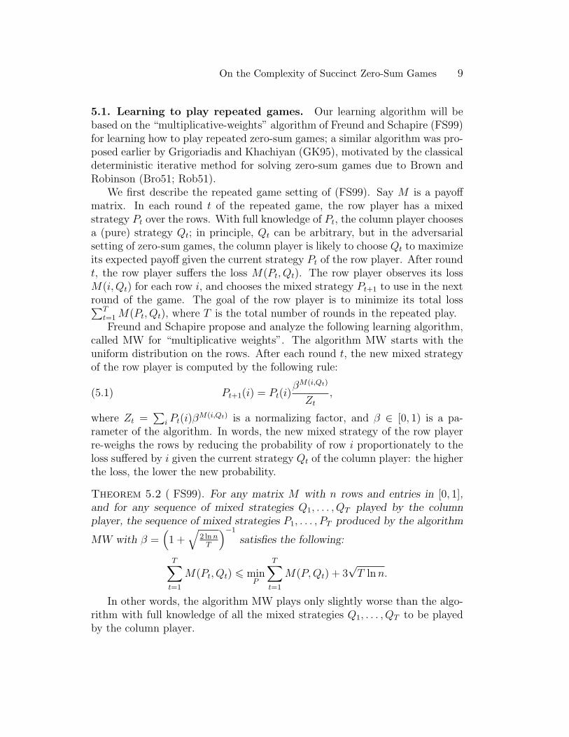
5.1. Learning to play repeated games. Our learning algorithm will bebased on the “multiplicative-weights” algorithm of Freund and Schapire (FS99)for learning how to play repeated zero-sum games; a similar algorithm was pro-posed earlier by Grigoriadis and Khachiyan (GK95), motivated by the classicaldeterministic iterative method for solving zero-sum games due to Brown andRobinson (Bro51; Rob51).

We first describe the repeated game setting of (FS99). Say M is a payoffmatrix. In each round t of the repeated game, the row player has a mixedstrategy Pt over the rows. With full knowledge of Pt, the column player choosesa (pure) strategy Qt; in principle, Qt can be arbitrary, but in the adversarialsetting of zero-sum games, the column player is likely to choose Qt to maximizeits expected payoff given the current strategy Pt of the row player. After roundt, the row player suffers the loss M(Pt, Qt). The row player observes its lossM(i, Qt) for each row i, and chooses the mixed strategy Pt+1 to use in the nextround of the game. The goal of the row player is to minimize its total loss∑T

t=1M(Pt, Qt), where T is the total number of rounds in the repeated play.Freund and Schapire propose and analyze the following learning algorithm,

called MW for “multiplicative weights”. The algorithm MW starts with theuniform distribution on the rows. After each round t, the new mixed strategyof the row player is computed by the following rule:

(5.1) Pt+1(i) = Pt(i)βM(i,Qt)

Zt,

where Zt =∑

i Pt(i)βM(i,Qt) is a normalizing factor, and β ∈ [0, 1) is a pa-

rameter of the algorithm. In words, the new mixed strategy of the row playerre-weighs the rows by reducing the probability of row i proportionately to theloss suffered by i given the current strategy Qt of the column player: the higherthe loss, the lower the new probability.

Theorem 5.2 ( FS99). For any matrix M with n rows and entries in [0, 1],and for any sequence of mixed strategies Q1, . . . , QT played by the columnplayer, the sequence of mixed strategies P1, . . . , PT produced by the algorithm

MW with β =(

1 +√

2 lnnT

)−1

satisfies the following:

T∑t=1

M(Pt, Qt) 6 minP

T∑t=1

M(P,Qt) + 3√T lnn.

In other words, the algorithm MW plays only slightly worse than the algo-rithm with full knowledge of all the mixed strategies Q1, . . . , QT to be playedby the column player.

10 Fortnow et al.

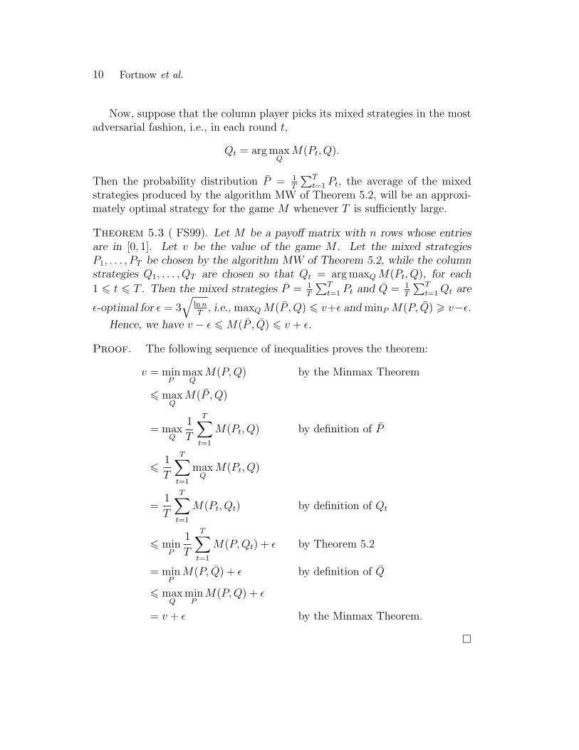
Now, suppose that the column player picks its mixed strategies in the mostadversarial fashion, i.e., in each round t,

Qt = arg maxQ

M(Pt, Q).

Then the probability distribution P = 1T

∑Tt=1 Pt, the average of the mixed

strategies produced by the algorithm MW of Theorem 5.2, will be an approxi-mately optimal strategy for the game M whenever T is sufficiently large.

Theorem 5.3 ( FS99). Let M be a payoff matrix with n rows whose entriesare in [0, 1]. Let v be the value of the game M . Let the mixed strategiesP1, . . . , PT be chosen by the algorithm MW of Theorem 5.2, while the columnstrategies Q1, . . . , QT are chosen so that Qt = arg maxQM(Pt, Q), for each

1 6 t 6 T . Then the mixed strategies P = 1T

∑Tt=1 Pt and Q = 1

T

∑Tt=1Qt are

ε-optimal for ε = 3√

lnnT

, i.e., maxQM(P , Q) 6 v+ε and minP M(P, Q) > v−ε.Hence, we have v − ε 6M(P , Q) 6 v + ε.

Proof. The following sequence of inequalities proves the theorem:

v = minP

maxQ

M(P,Q) by the Minmax Theorem

6 maxQ

M(P , Q)

= maxQ

1

T

T∑t=1

M(Pt, Q) by definition of P

61

T

T∑t=1

maxQ

M(Pt, Q)

=1

T

T∑t=1

M(Pt, Qt) by definition of Qt

6 minP

1

T

T∑t=1

M(P,Qt) + ε by Theorem 5.2

= minPM(P, Q) + ε by definition of Q

6 maxQ

minPM(P,Q) + ε

= v + ε by the Minmax Theorem.

�


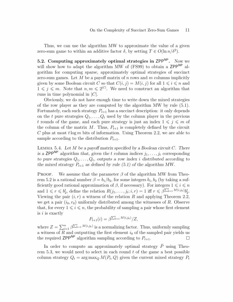
Thus, we can use the algorithm MW to approximate the value of a givenzero-sum game to within an additive factor δ, by setting T ∈ O(lnn/δ2).

5.2. Computing approximately optimal strategies in ZPPNP. Now wewill show how to adapt the algorithm MW of (FS99) to obtain a ZPPNP al-gorithm for computing sparse, approximately optimal strategies of succinctzero-sum games. Let M be a payoff matrix of n rows and m columns implicitlygiven by some Boolean circuit C so that C(i, j) = M(i, j) for all 1 6 i 6 n and1 6 j 6 m. Note that n,m 6 2|C|. We need to construct an algorithm thatruns in time polynomial in |C|.

Obviously, we do not have enough time to write down the mixed strategiesof the row player as they are computed by the algorithm MW by rule (5.1).Fortunately, each such strategy Pt+1 has a succinct description: it only dependson the t pure strategies Q1, . . . , Qt used by the column player in the previoust rounds of the game, and each pure strategy is just an index 1 6 j 6 m ofthe column of the matrix M . Thus, Pt+1 is completely defined by the circuitC plus at most t logm bits of information. Using Theorem 2.2, we are able tosample according to the distribution Pt+1.

Lemma 5.4. Let M be a payoff matrix specified by a Boolean circuit C. Thereis a ZPPNP algorithm that, given the t column indices j1, . . . , jt correspondingto pure strategies Q1, . . . , Qt, outputs a row index i distributed according tothe mixed strategy Pt+1 as defined by rule (5.1) of the algorithm MW.

Proof. We assume that the parameter β of the algorithm MW from Theo-rem 5.2 is a rational number β = b1/b2, for some integers b1, b2 (by taking a suf-ficiently good rational approximation of β, if necessary). For integers 1 6 i 6 n

and 1 6 r 6 bt2, define the relation R(j1, . . . , jt; i, r) = 1 iff r 6 βPt

k=1M(i,jk)bt2.Viewing the pair (i, r) a witness of the relation R and applying Theorem 2.2,we get a pair (i0, r0) uniformly distributed among the witnesses of R. Observethat, for every 1 6 i 6 n, the probability of sampling a pair whose first elementis i is exactly

Pt+1(i) = βPt

k=1M(i,jk)/Z,

where Z =∑n

i=1 βPt

k=1M(i,jk) is a normalizing factor. Thus, uniformly samplinga witness of R and outputting the first element i0 of the sampled pair yields usthe required ZPPNP algorithm sampling according to Pt+1. �

In order to compute an approximately optimal strategy P using Theo-rem 5.3, we would need to select in each round t of the game a best possiblecolumn strategy Qt = arg maxQM(Pt, Q) given the current mixed strategy Pt

12 Fortnow et al.

of the row player. It is not clear if this can be accomplished in BPPNP. How-ever, the proof of Theorem 5.3 can be easily modified to argue that if eachQt is chosen so that M(Pt, Qt) > maxQM(Pt, Q) − σ, for some σ > 0, thenthe resulting mixed strategies P and Q will be (ε + σ)-optimal (rather thanε-optimal). In other words, choosing in each round t an almost best possiblecolumn strategy Qt is sufficient for obtaining approximately optimal strategiesP and Q.

We now explain how to choose such almost best possible column strate-gies Qt in BPPNP. The reader should not be alarmed by the fact that we areconsidering a BPPNP algorithm, rather than a ZPPNP algorithm. This BPPNP

algorithm will only be used as a subroutine in our final, error-free ZPPNP algo-rithm.

Fix round t, 1 6 t 6 T . We assume that we have already chosen strategiesQ1, . . . , Qt−1, and hence the mixed strategy Pt is completely specified; the basecase is for t = 1, where P1 is simply the uniform distribution over the rows ofthe matrix M .

Lemma 5.5. There is a BPPNP algorithm that, given column indices j1, . . . , jt−1

of the matrix M for t > 1 and σ > 0, outputs a column index jt such that,with high probability over the random choices of the algorithm, M(Pt, jt) >maxjM(Pt, j)−σ. The running time of the algorithm is polynomial in t, 1/σ, |C|,where C is the Boolean circuit that defines the matrix M .

Proof. Let σ′ = σ/2. For integer k to be specified later, form the multiset Sby sampling k times independently at random according to the distribution Pt;this can be achieved in ZPPNP by Lemma 5.4. For any fixed column 1 6 j 6 m,the probability that | 1

|S|∑

i∈SM(i, j) −M(Pt, j)| > σ′ is at most 2e−2kσ′2by

the Hoeffding bounds (Hoe63). Thus, with probability at least 1 − 2me−2kσ′2,

we have that | 1|S|∑

i∈SM(i, j) −M(Pt, j)| 6 σ′ for every column 1 6 j 6 m.

Let us call such a multiset S good. Choosing k ∈ poly(logm, 1/σ), we can makethe probability of constructing a good multiset S sufficiently high.

Assuming that we have constructed a good multiset S, we can now pick j =arg maxj

∑i∈SM(i, j) in PNP as follows. First, we compute w∗ = maxj

∑i∈SM(i, j)

by going through all possible integers w = 0, . . . , k, asking the NP-query: Isthere a column 1 6 j 6 m such that

∑i∈SM(i, j) > w? The required w∗

will be the last value of w for which our query is answered positively. (Tospeed up things a little, we could also do the binary search over the in-terval of integers between 0 and k.) Once we have computed w∗, we cando the binary search over the column indices 1 6 j 6 m, asking the NP-


query: Is there a column j in the upper half of the current interval suchthat

∑i∈SM(i, j) = w∗? After at most logm steps, we will get the re-

quired j∗ = arg maxj∑

i∈SM(i, j). Finally, since S is a good set, we have thatM(Pt, j

∗) > 1|S|∑

i∈SM(i, j∗)−σ′ > maxjM(Pt, j)− 2σ′ = maxjM(Pt, j)−σ,as promised. �

Running the BPPNP algorithm of Lemma 5.5 for T ∈ O(lnn/σ2) steps,we construct a sequences of pure strategies Q1, . . . , QT such that, with highprobability over the random choices of the algorithm, the mixed strategiesP = 1

T

∑Tt=1 Pt (determined by rule (5.1)) and Q = 1

T

∑Tt=1Qt are 2σ-optimal.

That is, maxQM(P , Q) 6 v + 2σ and minP M(P, Q) > v − 2σ, where v is thevalue of the game M . Hence, we have with high probability that v − 2σ 6M(P , Q) 6 v + 2σ.

Since both the mixed strategies P and Q have small descriptions, they bothcan be sampled by a ZPPNP algorithm. The case of Q is trivial since it is asparse strategy on at most T columns. To sample from P , we pick 1 6 t 6 Tuniformly at random, sample from Pt using the algorithm of Lemma 5.4, andoutput the resulting row index.

Finally, we can prove the main theorem of this section.

Theorem 5.6. There is a ZPPNP algorithm that, given a δ > 0 and Booleancircuit C defining a payoff matrix M of unknown value v, outputs a numberu and multisets S1 and S2 of row and column indices, respectively, such that|S1| = k1 and |S2| = k2 for k1, k2 ∈ poly(|C|, 1/δ),

v − δ 6 u 6 v + δ,

and the multisets S1 and S2 give rise to sparse approximately optimal strategies,i.e.,

maxj

1

k1

∑i∈S1

M(i, j) 6 v + δ,

and

mini

1

k2

∑j∈S2

M(i, j) > v − δ.

The running time of the algorithm is polynomial in |C| and 1/δ.

Proof. Let us set σ = δ/12. As explained in the discussion preceding thetheorem, we can construct in BPPNP the descriptions of two mixed strategiesP and Q such that v − 2σ 6 M(P , Q) 6 v + 2σ, where the running time ofthe BPPNP algorithm is poly(|C|, 1/σ). That is, with high probability, both

14 Fortnow et al.

the strategies are approximately optimal to within the additive factor 2σ. LetS2 be the multiset of column indices given by the sequence of pure strategiesQ1, . . . , QT used to define Q, where T = k2 ∈ poly(|C|, 1/σ). To construct S1,we sample from P independently k1 times. Obviously, both multisets can beconstructed in ZPPNP.

By uniformly sampling from S1, we can approximate M(P , Q) to withinan additive factor σ in probabilistic poly(|C|, 1/σ) time with high probability,by the Hoeffding bounds (Hoe63). That is, with high probability, the resultingestimate u will be such that v−3σ 6 u 6 v+3σ, and the sparse mixed strategiesgiven by S1 and S2 will be approximately optimal to within the additive factor3σ.

Finally, we show how to eliminate the error of our probabilistic construction.Given the estimate u and the sparse strategies S1 and S2, we can test in PNP

whether

(5.7) maxj

1

|S1|∑i∈S1

M(i, j) 6 u+ 6σ,

and

(5.8) mini

1

|S2|∑j∈S2

M(i, j) > u− 6σ.

If both tests (5.7) and (5.8) succeed, then we output u, S1, and S2; otherwise,we output Fail.

To analyze correctness, we observe that, with high probability, u, S1, andS2 are such that v − 3σ 6 u 6 v + 3σ,

maxj

1

|S1|∑i∈S1

M(i, j) 6 v + 3σ 6 u+ 6σ,

and, similarly,

mini

1

|S2|∑j∈S2

M(i, j) > v − 3σ > u− 6σ.

Hence, with high probability, our tests (5.7) and (5.8) will succeed. Wheneverthey succeed, the output u will approximate the value v of the game M towithin the additive factor 6σ < δ, while the sparse strategies given by S1 andS2 will be approximately optimal to within the additive factor 12σ = δ, asrequired. �


5.3. Applications. In this section, we show how our Theorem 4.1 and The-orem 5.6 can be used to derive several old and new results in a very uniformfashion.

Theorem 5.9 ( RS98). MA ⊆ Sp2

Proof. Let L ∈ MA be any language. As we argued in Section 1.2 of theIntroduction, for every x there is a succinct zero-sum game Mx defined by aBoolean circuit Cx such that the value of Mx is at least 2/3 if x ∈ L, and is atmost 1/3 if x 6∈ L.

Let us associate with every x the triple (Cx, 1/2, 18) in the format of in-

stances of SGV. By Theorem 4.1, the resulting problem SGV is in promise-Sp2,defined by some polynomial-time predicate R. Defining the new predicate

R(x, y, z)def= R((Cx, 1/2, 1

8), y, z) shows that L ∈ Sp2, as required. �

Theorem 5.10 ( Cai07). Sp2 ⊆ ZPPNP

Proof. Let L ∈ Sp2 be any language. As we argued in Section 1.2 of the In-troduction, the definition of Sp2 implies that for every x there exists a succinctzero-sum game whose value is 1 if x ∈ L, and is 0 if x 6∈ L. Since approximat-ing the value of any succinct zero-sum game to within a 1/4 is in ZPPNP byTheorem 5.6, the result follows. �

Remark 5.11. There are some connections between our results and those in(Cai07). Cai’s result and Lemma 4.3 together imply that the promise problemSGV is in ZPPNP, because the main proof in (Cai07) shows that promise-Sp2is in ZPPNP. Our Theorem 5.6 also shows that SGV is in ZPPNP, but goesfurther by also producing approximately optimal strategies. Because SGV isSP2 -hard, one of the consequences of our result is the alternative proof of Cai’smain result (Theorem 5.10) above.

It may also be possible to adapt Cai’s algorithm (or the similar algorithmof (BCG+96)) to give an alternative proof of Theorem 5.6. The implicit ver-sion of the Multiplicative Weights algorithm that we use seems more natu-ral, though, in a setting in which one wishes to recover approximately optimalstrategies. To adapt Cai’s algorithm for this purpose would presumably requireadditional pre-processing of the input so that the multisets obtained when thealgorithm halts can be converted into probability distributions representingapproximately optimal strategies.

16 Fortnow et al.

The proofs of the following results utilize the notion of a zero-sum gamebetween algorithms and inputs proposed by Yao (Yao77; Yao83).

Theorem 5.12 ( BCG+96). If SAT is in P/poly then there is a ZPPNP algo-rithm for learning polynomial-size circuits for SAT.

Proof. Let s′(n) ∈ poly(n) be the size of a Boolean circuit deciding thesatisfiability of any size-n Boolean formula. By the well-known self-reducibilityproperty of SAT, we get the existence of size s(n) ∈ poly(s′(n)) circuits that,given a Boolean formula φ of size n as input, output either False or a truthassignment for φ. If we start with a correct circuit for SAT, then the resultingcircuit for the search version of SAT will be such that it outputs False iffthe given formula φ is unsatisfiable, and outputs a satisfying assignment for φotherwise.

For any n, consider the succinct zero-sum game given by the payoff matrixM whose rows are labeled by circuits C of size s(n), and whose columns arelabeled by the pairs (φ, x) where φ is a Boolean formula of size n and x is anassignment to the variables of φ. We define

M(C,(φ, x)) ={1 if φ(x) =True, and (C(φ) = False or C(φ) = y such that φ(y) =False)

0 otherwise.

In words, the matrix M is defined to penalize the row player for using incorrectcircuits for SAT.

By our assumption, there is a size-s(n) circuit C that correctly decides SAT.Hence, the row C of the matrix M will consist entirely of 0’s, and so the valuev of the game M is 0.

Applying Theorem 5.6 to the succinct zero-sum game M (with δ = 1/4),we obtain a ZPPNP algorithm for learning a size-k multiset S of circuits, fork ∈ poly(s(n)), such that, for every column j of M ,

1

|S|∑i∈S

M(i, j) 6 1/4.

This means that, for every satisfiable Boolean formula φ of size n, at least 3/4of the circuits in the multiset S will produce a satisfying assignment for φ.Therefore, the following polynomial-size Boolean circuit will correctly decideSAT: On input φ, output 1 iff at least one of the circuits in S produces asatisfying assignment for φ. �


Using similar ideas, we also obtain the following improvements on someresults from (LY94), which are implicit in (BCG+96).

Theorem 5.13 ( BCG+96). Let C be a Boolean circuit over n-bit inputs, andlet s be the size of the smallest possible Boolean circuit equivalent to C. Thereis a ZPPNP algorithm that, given a Boolean circuit C, outputs an equivalentcircuit of size O(ns+ n log n).

Proof. For every 1 6 i 6 |C|, consider the succinct zero-sum game with thepayoff matrix Mi whose rows are labeled by size-i Boolean circuit A and whosecolumns are labeled by n-bit strings x. We define Mi(A, x) = 0 if A(x) = C(x),and Mi(A, x) = 1 if A(x) 6= C(x).

Clearly, the value of the game Mi is 0 for all i > s. Applying the ZPPNP

algorithm of Theorem 5.6 to every i = 1, . . . , |C| in turn, we can find the firsti0 6 s such that the value of the game Mi0 is at most 1/4. Similarly to theproof of Theorem 5.12, we get a small multiset of size-i0 circuits such that theirmajority agrees with C on all inputs. It is not difficult to verify that the sizeof this constructed circuit is at most O(ni0 + n log n), as claimed. �

Theorem 5.13 can also be used to check in ZPPNP if a given Boolean circuitis approximately the smallest possible, i.e., if there is no equivalent circuit ofsignificantly smaller size.

6. Multiplicative-Factor Approximation

In the previous sections, we studied the problem of approximating the value ofa given succinct zero-sum game to within an additive factor. It is natural toconsider the problem of multiplicative-factor approximation: Given a Booleancircuit C computing the payoff matrix of a zero-sum game of unknown valuev, and a parameter ε (written in unary), compute w = (1± ε)v.

It follows from the work of Luby and Nisan (LN93) that approximatingthe value of a given succinct zero-sum game to within a multiplicative factor ε(written in unary) is in PSPACE. The result in (LN93) talks about explicitlygiven linear programming problems where the input constraint matrix and con-straint vector are positive; zero-sum games are a special case of such “positivelinear programming” problems. The algorithm in (LN93) uses a polynomialnumber of processors and runs in time polynomial in ε and polylogarithmic inthe size of the input matrix. By scaling it up, one obtains a PSPACE algorithmfor implicitly given zero-sum games.

18 Fortnow et al.

We do not know whether multiplicative-factor approximation of succinctzero-sum games can be done in the polynomial-time hierarchy. This is aninteresting open question. However, we can show that, unless the polynomial-time hierarchy collapses to the second level, multiplicative-factor approximationis strictly harder than additive-factor approximation.

Theorem 6.1. If the value of every succinct zero-sum game can be approxi-mated to within some multiplicative constant factor ε < 1 in Σp

2, then PH = Σp2.

The proof of Theorem 6.1 relies on the simple observation that if one couldapproximate the value of a game to within some constant factor ε < 1, thenone could tell if the value of the game is zero or not. In turn, this would allowone to decide every language in Πp

2. More formally, we have the following.

Lemma 6.2. The problem of approximating the value of a succinct zero-sumgame to within a multiplicative constant factor ε < 1 is Πp

2-hard.

Proof. Let L ∈ Πp2 be an arbitrary language, and let R be a polynomial-time

computable ternary relation such that, for all inputs x, x ∈ L⇔ ∀y∃zR(x, y, z),where |y| and |z| are polynomial in |x|. For every input x, consider the followingzero-sum game Mx:

Mx(y, z) =

{1 if R(x, y, z) is true

0 otherwise.

We claim that if x ∈ L, then the value of the game Mx is greater than0; and if x 6∈ L, then the value of Mx is 0. Indeed, if x 6∈ L, then the rowplayer has a pure strategy y that achieves the payoff 0 for any strategy z ofthe column player. On the other hand, if x ∈ L, then the uniform distributionover the columns achieves the payoff at least 2−|z| > 0 for any strategy y of therow player.

It follows that an algorithm for approximating the value of a succinct zero-sum game to within a multiplicative factor ε < 1 can be used to decide thelanguage L, which proves the lemma. �

Proof (Proof of Theorem 6.1). By the assumption of the theorem and byLemma 6.2, we get that Πp

2 ⊆ Σp2, implying the collapse PH = Σp

2. �


7. Learning approximately optimal strategies in PNP?

The learning algorithm we presented in Section 5.2 is randomized. It is nat-ural to ask whether it can be efficiently derandomized. Here we observe thatachieving such derandomization is likely to be fairly difficult as it would implynew strong circuit lower bounds. More precisely, we have the following.

Theorem 7.1. If there is a PNP algorithm for approximating the value of anygiven succinct zero-sum game to within an additive factor, then EXPNP 6⊂P/poly.

For the proof of Theorem 7.1, we will need the following results.

Theorem 7.2 ( BH92). If EXPNP ⊂ P/poly, then EXPNP = EXP.

Theorem 7.3 ( BFL91). If EXP ⊂ P/poly, then EXP = MA.

Proof (Proof of Theorem 7.1). Our proof is by contradiction. If EXPNP ⊂P/poly, then EXPNP = EXP = MA ⊆ Sp2 by combining Theorem 7.2, Theo-rem 7.3, and Theorem 5.9. Since approximating the value of a succinct zero-sum game is complete for promise-Sp2 by Theorem 4.1, the assumed existence ofa PNP algorithm for that problem would imply the collapse Sp2 = PNP. Hence,we would get EXPNP = PNP, which is impossible by diagonalization. �

8. A Version of Succinct Set Cover isPromise-Sp

2-complete

In this Section, we demonstrate another natural problem that is complete forpromise-Sp2. Our problem is a variant of the Succinct Set Cover problem intro-duced by Umans (Uma99).

An instance of Succinct Set Cover (SSC) is given by a 0-1 incidence matrixA with rows (“sets”) indexed by {0, 1}m and columns (“elements”) indexed by{0, 1}n. The matrix is presented as a circuit C where C(i, j) outputs the (i, j)entry of A, which is 1 iff element j is in set i. The goal is to find the smallestset cover, i.e., a set I such that ∀j∃i ∈ I C(i, j) = 1.

We define the promise problem n/ log n-SSC whose positive instances are(C, 1k) such that there is a set cover of size at most k, and whose negativeinstances are (C, 1k) such that there is no set cover of size less than k(n/ log n).

20 Fortnow et al.

Theorem 8.1. n/ log n-SSC is promise-Sp2-complete.

Proof. First, it is promise-Sp2-hard. Given any relation R(x, y, z) defining apromise-Sp2 problem and an input x, just take A to be A(i, j) = R(x, i, j). IfR(x, y, z) has an all-1 row, then there is a set cover of size 1. If R(x, y, z) hasan all-0 column, then there is no set cover of any size.

Now we prove that n/ log n-SSC is in promise-Sp2. We are given an instance(C, 1k). The game matrix M has rows indexed by {0, 1}n and columns indexedby k-subsets of {0, 1}m. Entry M(i; j1, j2, . . . , jk) is 1 iff there is a 1 6 ` 6 kfor which C(j`, i) = 1.

It is clear that if we start with a positive instance, then there is an all-1column, and so the value of the game is 1. On the other hand, if we start witha negative instance, then there is no cover of size k(n/ log n), and we claimthat there exists a set I of rows with |I| = poly(n,m, k) such that ∀J∃i ∈I M(i; J) = 0. Thus, by playing the uniform distribution over the rows in I,the row player achieves the value at most 1− 1/|I|.

Now we prove our claim. First, observe that there must exist a i such thatPrJ [M(i; J) = 0] > 1/n. Indeed, suppose otherwise, i.e., that every i is coveredby a random column of M with probability greater than 1 − 1/n. Then theprobability that a fixed i is not covered by any of n/ log n columns of M , chosenindependently and uniformly at random, is less than 1/nn/ logn = 2−n. Thus,there exists a set of n/ log n columns of M that covers all i’s. This meansthat the original Succinct Set Cover instance has a set cover of size k(n/ log n),contradicting our assumption.

Let us add this i to our set I, and delete all columns J for which M(i; J) = 0.Repeating this procedure poly(n, k,m) times will eliminate all columns of M ,yielding the requisite set I. �

9. Conclusions

We have shown that the problem of approximating the value of a succinctlygiven zero-sum game is complete for the “promise” version of the class Sp2. Thisappears to be the first natural problem proved to capture the complexity of Sp2;however, it is not the only one, as demonstrated in Section 8.

We presented a ZPPNP algorithm for learning the approximate value andapproximately optimal sparse strategies for the given succinct zero-sum game.Our algorithm allowed us to prove a few results from (BCG+96; Cai07; LY94)in a completely uniform fashion, via the connection between zero-sum gamesand computational complexity discovered by Yao (Yao77; Yao83). Finally, we


also argued that our ZPPNP algorithm cannot be derandomized unless there isa major progress in proving circuit lower bounds for EXPNP.

Acknowledgements

We want to thank Joe Kilian for bringing (FKS95) to our attention, and Chris-tos Papadimitriou for answering our questions on linear programming and zero-sum games. We also thank David Zuckerman for helpful discussions, and theanonymous referees for their comments. Lance Fortnow acknowledges NECLaboratories America where he did the research reported in this paper. RussellImpagliazzo’s research was supported by NSF Award CCR-0098197 and USA-Israel BSF Grant 97-00188. Valentine Kabanets did most of this research whileat the University of California, San Diego, supported by an NSERC postdoc-toral fellowship. Chris Umans’s research was supported in part by NSF grantCCF-0346991.

References

[Alt94] I. Althofer. On sparse approximations to randomized strategies and con-vex combinations. Linear Algebra and its Applications, 199, 1994.

[Bab85] L. Babai. Trading group theory for randomness. In Proceedings of theSeventeenth Annual ACM Symposium on Theory of Computing, pages421–429, 1985.

[BCG+96] N.H. Bshouty, R. Cleve, R. Gavalda, S. Kannan, and C. Tamon. Oraclesand queries that are sufficient for exact learning. Journal of Computerand System Sciences, 52(3):421–433, 1996.

[BFL91] L. Babai, L. Fortnow, and C. Lund. Non-deterministic exponential timehas two-prover interactive protocols. Computational Complexity, 1:3–40,1991.

[BGP00] M. Bellare, O. Goldreich, and E. Petrank. Uniform generation of NP-witnesses using an NP-oracle. Information and Computation, 163:510–526, 2000.

[BH92] H. Buhrman and S. Homer. Superpolynomial circuits, almost sparse ora-cles and the exponential hierarchy. In R. Shyamasundar, editor, Proceed-ings of the Twelfth Conference on Foundations of Software Technologyand Theoretical Computer Science, volume 652 of Lecture Notes in Com-puter Science, pages 116–127, Berlin, Germany, 1992. Springer Verlag.

22 Fortnow et al.

[BM88] L. Babai and S. Moran. Arthur-Merlin games: A randomized proof sys-tem, and a hierarchy of complexity classes. Journal of Computer andSystem Sciences, 36:254–276, 1988.

[Bro51] G.W. Brown. Iterative solution of games by fictitious play. In T.C. Koop-mans, editor, Activity Analysis of Production and Allocation, volume 13of Cowles Commision Monograph, pages 129–136. Wiley, New York, 1951.

[Cai07] J.-Y. Cai. Sp2 is subset of ZPPNP. Journal of Computer and SystemSciences, 73(1):25–35, 2007.

[Can96] R. Canetti. On BPP and the polynomial-time hierarchy. InformationProcessing Letters, 57:237–241, 1996.

[FKS95] J. Feigenbaum, D. Koller, and P. Shor. A game-theoretic classification ofinteractive complexity classes. In Proceedings of the Tenth Annual IEEEConference on Computational Complexity, pages 227–237, 1995.

[FS96] Y. Freund and R.E. Schapire. Game theory, on-line prediction and boost-ing. In Proceedings of the Ninth Annual Conference on ComputationalLearning Theory, pages 325–332, 1996.

[FS99] Y. Freund and R.E. Schapire. Adaptive game playing using multiplicativeweights. Games and Economic Behavior, 29:79–103, 1999.

[GHR92] M. Goldmann, J. Hastad, and A. Razborov. Majority gates vs. generalweighted threshold gates. Computational Complexity, 2:277–300, 1992.

[GK92] M.D. Grigoriadis and L.G. Khachiyan. Approximate solution of matrixgames in parallel. In P.M. Pardalos, editor, Advances in Optimizationand Parallel Computing, pages 129–136. Elsevier, Amsterdam, 1992.

[GK95] M.D. Grigoriadis and L.G. Khachiyan. A sublinear-time randomized ap-proximation algorithm for matrix games. Operations Research Letters,18(2):53–58, 1995.

[Hoe63] W. Hoeffding. Probability inequalities for sums of bounded random vari-ables. American Statistical Journal, pages 13–30, 1963.

[Imp95] R. Impagliazzo. Hard-core distributions for somewhat hard problems. InProceedings of the Thirty-Sixth Annual IEEE Symposium on Foundationsof Computer Science, pages 538–545, 1995.

[JVV86] M. Jerrum, L.G. Valiant, and V.V. Vazirani. Random generation of com-binatorial structuress from a uniform distribution. Theoretical ComputerScience, 43:169–188, 1986.


[LN93] M. Luby and N. Nisan. A parallel approximation algorithm for positivelinear programming. In Proceedings of the Twenty-Fifth Annual ACMSymposium on Theory of Computing, pages 448–457, 1993.

[LY94] R.J. Lipton and N.E. Young. Simple strategies for large zero-sum gameswith applications to complexity theory. In Proceedings of the Twenty-Sixth Annual ACM Symposium on Theory of Computing, pages 734–740,1994.

[Neu28] J. von Neumann. Zur Theorie der Gesellschaftspiel. Mathematische An-nalen, 100:295–320, 1928.

[New91] I. Newman. Private vs. common random bits in communication complex-ity. Information Processing Letters, 39:67–71, 1991.

[Owe82] G. Owen. Game Theory. Academic Press, 1982.

[Pap94] C.H. Papadimitriou. Computational Complexity. Addison-Wesley, Read-ing, Massachusetts, 1994.

[PST95] S.A. Plotkin, D.B. Shmoys, and E. Tardos. Fast approximation algo-rithms for fractional packing and covering problems. Mathematics ofOperations Research, 20(2):257–301, 1995.

[Rob51] J. Robinson. An iterative method of solving a game. Annals of Mathe-matics, 54:296–301, 1951.

[RS98] A. Russell and R. Sundaram. Symmetric alternation captures BPP. Com-putational Complexity, 7(2):152–162, 1998.

[Uma99] C. Umans. Hardness of approximating Σp2 minimization problems. In

Proceedings of the Fortieth Annual IEEE Symposium on Foundations ofComputer Science, pages 465–474, 1999.

[Yao77] A.C. Yao. Probabilistic complexity: Towards a unified measure of com-plexity. In Proceedings of the Eighteenth Annual IEEE Symposium onFoundations of Computer Science, pages 222–227, 1977.

[Yao82] A.C. Yao. Theory and applications of trapdoor functions. In Proceed-ings of the Twenty-Third Annual IEEE Symposium on Foundations ofComputer Science, pages 80–91, 1982.

[Yao83] A.C. Yao. Lower bounds by probabilistic arguments. In Proceedings of theTwenty-Fourth Annual IEEE Symposium on Foundations of ComputerScience, pages 420–428, 1983.

24 Fortnow et al.

Manuscript received 11 October 2005

Lance FortnowDepartment of Computer ScienceUniversity of ChicagoChicago, [email protected]

Russell ImpagliazzoDepartment of Computer ScienceUniversity of California - San DiegoLa Jolla, [email protected]

Valentine KabanetsSchool of Computing ScienceSimon Fraser UniversityVancouver, [email protected]

Christopher UmansDepartment of Computer ScienceCalifornia Institute of TechnologyPasadena, [email protected]

Documents

ON THE COMPLEXITY OF SUCCINCT ZERO-SUM …fortnow/papers/succinct.pdfON THE COMPLEXITY OF SUCCINCT ZERO-SUM GAMES ... a variant of the Succinct Set Cover ... ZPP, BPP, PH, EXP, and