Digital Object Identifier (DOI) 10.1007/s10107-005-0653-9

Math. Program., Ser. B 105, 275–288 (2006)

Dirk Müller

On the complexity of the planar directed edge-disjoint pathsproblem

Received: April 1, 2004 / Accepted: May 10, 2005Published online: October 12, 2005 – © Springer-Verlag 2005

Abstract. The edge-disjoint paths problem and many special cases of it are known to be NP-complete. Wepresent a new NP-completeness result for a special case of the problem, namely the directed edge-disjointpaths problem restricted to planar supply graphs and demand graphs consisting of two sets of parallel edges.

Key words. Edge-disjoint paths – Planar graphs – Integral two-commodity-flows – NP-completeness –Complexity

1. Introduction

Given a (directed or undirected) supply graph G = (V , E) with vertex set V and edgeset E, and a demand graph H = (V , F ) on the same vertex set, the edge-disjoint pathsproblem consists in finding |F | (directed) edge-disjoint cycles in G+H (denoting theunion of G and H ), each containing exactly one edge in F .

It is well known that the edge-disjoint paths problem is NP-complete, in the generalcase (shown by Karp [2]) as well as in many important special cases. There is an exten-sive literature covering the complexity of the problem under various restrictions, a goodoverview is presented e. g. by Schrijver in part VII of [9]. Of course the edge-disjointpaths problem has many important applications.

The (directed and undirected) edge-disjoint paths problem is known to be NP-complete even when the demand graph H consists of two sets of parallel edges (seeEven, Itai and Shamir [1]). Kramer and van Leeuwen [5] showed that the edge-disjointpaths problem remains NP-complete if G is an undirected rectangular grid, implyingNP-completeness for general planar supply graphs G both in the directed and undirectedcase. Indeed, even if G + H is planar, the problem is NP-complete (Middendorf andPfeiffer [7]), again both in the directed and the undirected case.

While the undirected planar edge-disjoint paths problem with planar G + H isknown to be solvable in polynomial time if the demand edges cover only a fixed numberof vertices (shown by Sebo [10]), and Korach and Penn [3] even found an O(n

√log n)

algorithm for H consisting of two sets of parallel edges, the status of the planar directededge-disjoint paths problem under these conditions is still open. Also for planar G, but

D. Müller: Research Institute for Discrete Mathematics, University of Bonn, Lennestr. 2, 53113 Bonn,Germany. e-mail: mueller@or.uni-bonn.de

Mathematics Subject Classification (2000): 05C38, 68Q17, 68R10, 90C35

276 D. Müller

G+H not required to be planar, nothing was known so far about the complexity of theproblem if the demand edges cover only a fixed number of vertices.

In this article, we show the following:

Theorem 1. Let (G, H) be an instance of the directed edge-disjoint paths problemwith G being planar and H consisting of two sets of parallel edges. Then decidingif there is a solution to (G, H) is NP-complete.

If the number of demand edges is fixed (counting parallel edges with multiplicity),the status of the problem remains open, however. It should be noted that the planardirected vertex-disjoint paths problem with a fixed number of demand edges has beenshown to be solvable in polynomial time by Schrijver [8].

The outline of the proof of theorem 1 is as follows. As in [7], we will use a reductionfrom Planar 3SAT. We start with showing some basic transformation steps in section2, which will allow us to make certain assumptions in our subsequent construction.In section 3 we transform Planar 3SAT instances to (integral) two-commodity flowinstances with certain global properties. Together with the properties of the gadgets bywhich we will replace the vertices of the resulting supply graph in section 4, this enablesus to prove that the integral two-commodity-flow problem that we obtain in this way(or the equivalent edge-disjoint paths problem) has a solution if and only if the originalPlanar 3SAT instance is satisfiable.

We use standard notation as it is introduced for example in [4]. V (G) denotes thevertex set of a graph G, E(G) its edge set, and we write G = (V (G), E(G)). For anundirected graph G and two vertives v, w ∈ V (G), {v, w} denotes an edge connect-ing these vertices. In a directed graph, (v, w) denotes an edge oriented from v to w.For X ⊆ V (G), we define δ(X) := {{v, w} : v ∈ X, w ∈ V (G) \ X} in the undi-rected case. In the directed case, let δ+(X) := {(v, w) : v ∈ X, w ∈ V (G) \ X},δ−(X) := {(w, v) : v ∈ X, w ∈ V (G) \ X}, and δ(X) := δ+(X) ∪ δ−(X). We writeδ(v) := δ({v}).

For an undirected graph G, let G[X] := (X, E(G) ∩ {{v, w} : v, w ∈ X}) (analo-gously for directed graphs), and G− v := G[V (G)\{v}] for v ∈ V (G).

For an s-t-flow f : E(G) −→ R+0 in a directed graph G, s, t ∈ V (G), we define

f (J ) :=∑e∈J f (e) for a subset J ⊆ E(G) and |f | := f (δ+({s}))− f (δ−({s})).

2. Basic reduction steps

Definition 1. For B ∈ 3SAT, B = ∧i∈I ci , ci =

∨j∈Ji

lj , lj ∈ {vj , vj } for eachj , let G(B) := (V , E) be the graph of B, with I and Ji (i ∈ I ) being index sets,V := {ci : i ∈ I } ∪ {

vj : i ∈ I, j ∈ Ji

}and E := {{

ci, vj

}: i ∈ I, j ∈ Ji

}. We call

the vertices corresponding to variables V white vertices and the vertices correspondingto clauses black vertices. The Planar 3SAT problem is 3SAT restricted to instances B

with planar G(B).

Lichtenstein [6] has shown that Planar 3SAT is NP-complete. As shown in [7],the problem remains NP-complete when each variable is allowed to occur in at mostthree clauses: For an instance B ∈ Planar 3SAT, take a planar embedding of G(B). If

On the complexity of the planar directed edge-disjoint paths problem 277

c1

b1

a2a1

2

c2

c

c

c

3

4

5

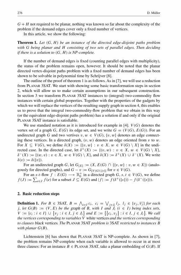
b

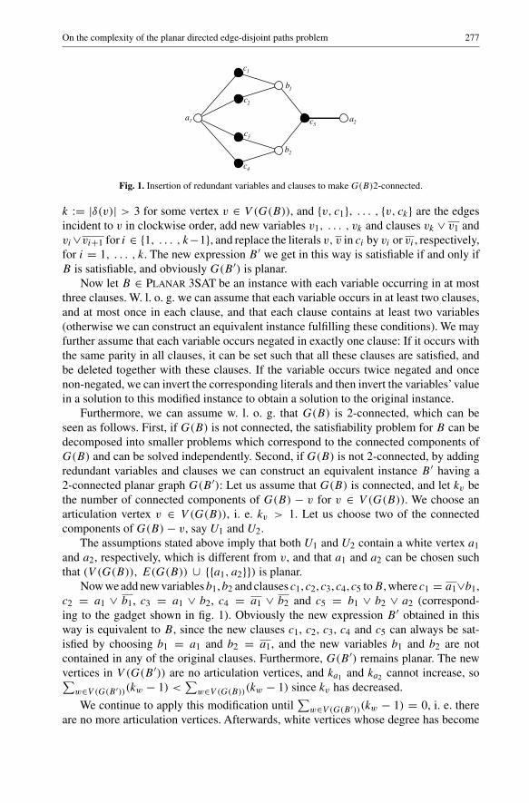
Fig. 1. Insertion of redundant variables and clauses to make G(B)2-connected.

k := |δ(v)| > 3 for some vertex v ∈ V (G(B)), and {v, c1}, . . . , {v, ck} are the edgesincident to v in clockwise order, add new variables v1, . . . , vk and clauses vk ∨ v1 andvi∨vi+1 for i ∈ {1, . . . , k−1}, and replace the literals v, v in ci by vi or vi , respectively,for i = 1, . . . , k. The new expression B ′ we get in this way is satisfiable if and only ifB is satisfiable, and obviously G(B ′) is planar.

Now let B ∈ Planar 3SAT be an instance with each variable occurring in at mostthree clauses. W. l. o. g. we can assume that each variable occurs in at least two clauses,and at most once in each clause, and that each clause contains at least two variables(otherwise we can construct an equivalent instance fulfilling these conditions). We mayfurther assume that each variable occurs negated in exactly one clause: If it occurs withthe same parity in all clauses, it can be set such that all these clauses are satisfied, andbe deleted together with these clauses. If the variable occurs twice negated and oncenon-negated, we can invert the corresponding literals and then invert the variables’valuein a solution to this modified instance to obtain a solution to the original instance.

Furthermore, we can assume w. l. o. g. that G(B) is 2-connected, which can beseen as follows. First, if G(B) is not connected, the satisfiability problem for B can bedecomposed into smaller problems which correspond to the connected components ofG(B) and can be solved independently. Second, if G(B) is not 2-connected, by addingredundant variables and clauses we can construct an equivalent instance B ′ having a2-connected planar graph G(B ′): Let us assume that G(B) is connected, and let kv bethe number of connected components of G(B) − v for v ∈ V (G(B)). We choose anarticulation vertex v ∈ V (G(B)), i. e. kv > 1. Let us choose two of the connectedcomponents of G(B)− v, say U1 and U2.

The assumptions stated above imply that both U1 and U2 contain a white vertex a1and a2, respectively, which is different from v, and that a1 and a2 can be chosen suchthat (V (G(B)), E(G(B)) ∪ {{a1, a2}}) is planar.

Now we add new variablesb1,b2 and clauses c1, c2, c3, c4, c5 toB, where c1 = a1∨b1,c2 = a1 ∨ b1, c3 = a1 ∨ b2, c4 = a1 ∨ b2 and c5 = b1 ∨ b2 ∨ a2 (correspond-ing to the gadget shown in fig. 1). Obviously the new expression B ′ obtained in thisway is equivalent to B, since the new clauses c1, c2, c3, c4 and c5 can always be sat-isfied by choosing b1 = a1 and b2 = a1, and the new variables b1 and b2 are notcontained in any of the original clauses. Furthermore, G(B ′) remains planar. The newvertices in V (G(B ′)) are no articulation vertices, and ka1 and ka2 cannot increase, so∑

w∈V (G(B ′))(kw − 1) <∑

w∈V (G(B))(kw − 1) since kv has decreased.

We continue to apply this modification until∑

w∈V (G(B ′))(kw − 1) = 0, i. e. thereare no more articulation vertices. Afterwards, white vertices whose degree has become

278 D. Müller

Fig. 2.

greater than three can be replaced as described above so that each white vertex has adegree of at most three again; this operation preserves planarity and 2-connectedness.

3. Construction of planar integral two-commodity flow instances

In this section, given an instance B of Planar 3SAT fulfilling the assumptions statedabove, we construct a directed integral two-commodity flow instance with a planar sup-ply graph having certain global properties which will help us to prove theorem 1 in thenext section.

The supply graph that we construct from G(B) will be called G′(B) = (V ′, E′1 ∪E′2 ∪ E′3), with V ′ := V ∪ {s, t} and E′1 := {

(vj , ci) : i ∈ I, j ∈ Ji

}, i. e. we orient

the edges in E(G(B)) from white to black vertices. We assume a planar embedding ofG(B), and for the vertices in V ′ \ {s, t} and the edges in E′1 we keep the embedding oftheir counterparts in G(B). We place the new vertex s within the outer face of G′(B)

and choose some other face F within which we place t . We colour s white and t black.

Definition 2. We say that an edge (v, c) ∈ E′1 is negative if the variable v occurs negatedin the clause c, and that it is positive otherwise.

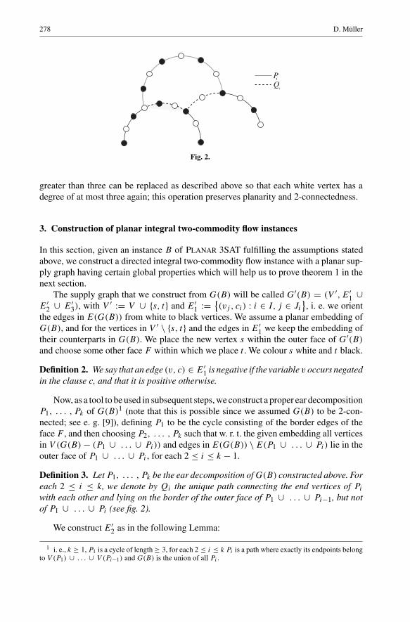
Now, as a tool to be used in subsequent steps, we construct a proper ear decompositionP1, . . . , Pk of G(B)1 (note that this is possible since we assumed G(B) to be 2-con-nected; see e. g. [9]), defining P1 to be the cycle consisting of the border edges of theface F , and then choosing P2, . . . , Pk such that w. r. t. the given embedding all verticesin V (G(B)− (P1 ∪ . . . ∪ Pi)) and edges in E(G(B)) \E(P1 ∪ . . . ∪ Pi) lie in theouter face of P1 ∪ . . . ∪ Pi , for each 2 ≤ i ≤ k − 1.

Definition 3. Let P1, . . . , Pk be the ear decomposition of G(B) constructed above. Foreach 2 ≤ i ≤ k, we denote by Qi the unique path connecting the end vertices of Pi

with each other and lying on the border of the outer face of P1 ∪ . . . ∪ Pi−1, but notof P1 ∪ . . . ∪ Pi (see fig. 2).

We construct E′2 as in the following Lemma:

1 i. e., k ≥ 1, P1 is a cycle of length≥ 3, for each 2 ≤ i ≤ k Pi is a path where exactly its endpoints belongto V (P1) ∪ . . . ∪ V (Pi−1) and G(B) is the union of all Pi .

On the complexity of the planar directed edge-disjoint paths problem 279

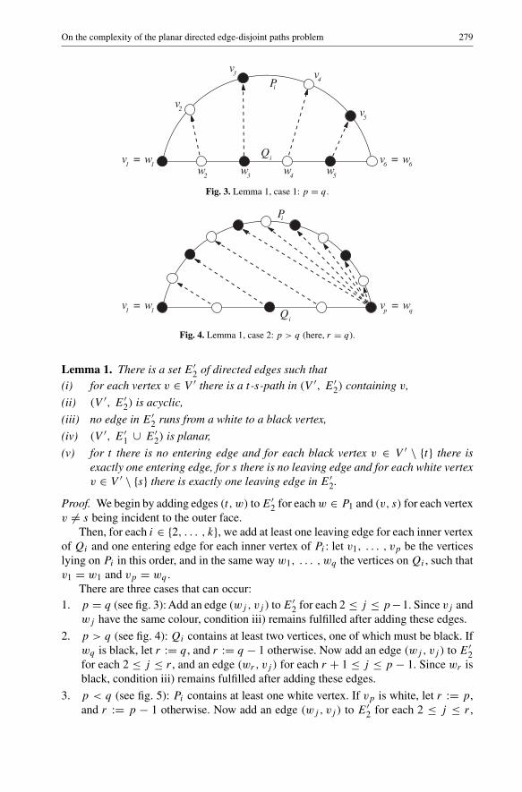
Fig. 3. Lemma 1, case 1: p = q.

Fig. 4. Lemma 1, case 2: p > q (here, r = q).

Lemma 1. There is a set E′2 of directed edges such that(i) for each vertex v ∈ V ′ there is a t-s-path in (V ′, E′2) containing v,

(ii) (V ′, E′2) is acyclic,

(iii) no edge in E′2 runs from a white to a black vertex,

(iv) (V ′, E′1 ∪ E′2) is planar,

(v) for t there is no entering edge and for each black vertex v ∈ V ′ \ {t} there isexactly one entering edge, for s there is no leaving edge and for each white vertexv ∈ V ′ \ {s} there is exactly one leaving edge in E′2.

Proof. We begin by adding edges (t, w) to E′2 for each w ∈ P1 and (v, s) for each vertexv �= s being incident to the outer face.

Then, for each i ∈ {2, . . . , k}, we add at least one leaving edge for each inner vertexof Qi and one entering edge for each inner vertex of Pi : let v1, . . . , vp be the verticeslying on Pi in this order, and in the same way w1, . . . , wq the vertices on Qi , such thatv1 = w1 and vp = wq .

There are three cases that can occur:1. p = q (see fig. 3): Add an edge (wj , vj ) to E′2 for each 2 ≤ j ≤ p−1. Since vj and

wj have the same colour, condition iii) remains fulfilled after adding these edges.

2. p > q (see fig. 4): Qi contains at least two vertices, one of which must be black. Ifwq is black, let r := q, and r := q − 1 otherwise. Now add an edge (wj , vj ) to E′2for each 2 ≤ j ≤ r , and an edge (wr, vj ) for each r + 1 ≤ j ≤ p − 1. Since wr isblack, condition iii) remains fulfilled after adding these edges.

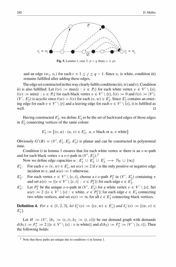
3. p < q (see fig. 5): Pi contains at least one white vertex. If vp is white, let r := p,and r := p − 1 otherwise. Now add an edge (wj , vj ) to E′2 for each 2 ≤ j ≤ r ,

280 D. Müller

Fig. 5. Lemma 1, case 3: p < q (here, r = p).

and an edge (wj , vr) for each r + 1 ≤ j ≤ q − 1. Since vr is white, condition iii)remains fulfilled after adding these edges.

The edge set constructed in this way clearly fulfils conditions iii), iv) and v). Conditionii) is also fulfilled: Let l(v) := max{i : v ∈ Pi} for each white vertex v ∈ V ′ \ {s},l(v) := min{i : v ∈ Pi} for each black vertex v ∈ V ′ \ {t}, l(t) := 0 and l(s) := |V ′|.(V ′, E′2) is acyclic since l(w) > l(v) for each (v, w) ∈ E′2. Since E′2 contains an enter-ing edge for each v ∈ V ′ \ {t} and a leaving edge for each v ∈ V ′ \ {s}, i) is fulfilled aswell. �

Having constructed E′2, we define E′3 to be the set of backward edges of those edgesin E′2 connecting vertices of the same colour:

E′3 := {(v, u) : (u, v) ∈ E′2, u, v black or u, v white

}

Obviously G′(B) = (V ′, E′1, E′2, E

′3) is planar and can be constructed in polynomial

time.Condition i) in lemma 1 ensures that for each white vertex w there is an s-w-path

and for each black vertex v a v-t-path in (V ′, E′3).2

Now we define edge capacities u : E′1 ∪ E′2 ∪ E′3 −→ N0 ∪ {∞}:E′1: For each e = (v, w) ∈ E′1, set u(e) := 2 if e is the only positive or negative edge

incident to v, and u(e) := 1 otherwise.

E′2: For each vertex v ∈ V ′ \ {s, t}, choose a t-s-path P v2 in (V ′, E′2) containing v

and set u(e) := |{v ∈ V ′ \ {s, t} : e ∈ P v2 }| for each edge e ∈ E′2.

E′3: Let P v3 be the unique s-v-path in (V ′, E′3) for a white vertex v ∈ V ′ \ {s}. Set

u(e) := 2 |{v ∈ V ′ \ {s} : v white, e ∈ P v3 }| for each edge e ∈ E′3 connecting

two white vertices, and set u(e) := ∞ for all e ∈ E′3 connecting black vertices.

Definition 4. For x ∈ {1, 2, 3}, let δ+x (v) := {(v, w) ∈ E′x} and δ−x (v) := {(w, v) ∈E′x}.

Let H := (V ′, {h1 := (s, t), h2 := (t, s)}) be our demand graph with demandsd(h1) := F ∗1 := 2 |{v ∈ V ′ \ {s} : v is white}| and d(h2) := F ∗2 := |V ′ \ {s, t}|. Thenthe following holds:

2 Note that these paths are unique due to condition v) in lemma 1.

On the complexity of the planar directed edge-disjoint paths problem 281

Lemma 2. The integral two-commodity-flow problem given by (G′(B), H, u, d) has asolution, and each solution f1, f2 : E′1 ∪ E′2 ∪ E′3 −→ N0 (f2 being the flow meetingh2’s demand) satisfies the following conditions:i) f2(e) = u(e) for each edge e ∈ E′2,

ii) f2(e) = 0 for each edge e �∈ E′2,

In order to prove this, we first show the following:

Lemma 3. Let f : E′1 ∪ E′2 ∪ E′3 −→ N0 be a maximum t-s-flow in (G′(B), u). Thenwe havei) |f | = F ∗2 ,

ii) f (e) = u(e) for each e ∈ E′2,

iii) f (e) = 0 for each e ∈ E′1 ∪ E′3.

Proof. i) follows from the definition of the edge capacities, and since δ+(t) ⊆ E′2, theflow value cannot be greater.

Now let us introduce a topological ordering l : V ′ −→ N on the acyclic graph(V ′, E′2) with l(t) = 1 and l(s) = |V ′|.

The first step is to prove the claim only for the edges in G′(B) leaving black vertices,which we do by induction on the label l of the vertices: Obviously we have f (δ+2 (t)) =u(δ+2 (t)). Now let v be a black vertex with l(v) > 1. Due to condition iii) in lemma 1all edges in δ−2 (v) start at a black vertex, and by the topological ordering this vertexmust have a smaller l-value than v, so by induction we know that f (δ−2 (v)) = u(δ−2 (v)).Now let us assume that f (e) > 0 for some edge e = (v, w) ∈ E′3. Then w is black andl(w) < l(v), so again by induction we have f (δ+3 (w)) = 0 and f (δ+2 (w)) = u(δ+2 (w)).Since δ+1 (w) = ∅, this implies that if w = t , we must have |f | < F ∗2 , and if w �= t ,the flow condition cannot be fulfilled at the vertex w since f (δ−2 (w)) = f (δ+2 (w)). Sof (δ+3 (v)) = 0 and f (δ+2 (v)) = u(δ+2 (v)) since u(δ+2 (v)) = u(δ−2 (v)).

We now prove the claim for all edges in G′(B) leaving white vertices, again byinduction on the vertex labels l: Let v be a white vertex. Then we have f (δ−2 (v)) =u(δ−2 (v)) since δ−2 (v) contains only edges starting either at a black vertex or at a whitevertex w with l(w) < l(v). For those edges we have already shown that they are saturatedby f .

Now let us assume that f (e) > 0 for an edge e = (v, w) ∈ E′1 ∪ E′3, with w

being black. If w = t , then |f | < F ∗2 , and otherwise the flow condition cannot befulfilled at the vertex w. So we must have f (e) = 0. If now f (e) > 0 for an edgee = (v, w) ∈ E′3, with w being white, then by induction (since l(w) < l(v)) we havef (δ+2 (w)) = u(δ+2 (w)) and f (δ+1 (w) ∪ δ+3 (w)) = 0. So if f (e) > 0, again the flowcondition cannot be fulfilled at the vertex w, which implies f (δ+1 (v) ∪ δ+3 (v)) = 0 andf (δ+2 (v)) = u(δ+2 (v)). � Lemma 4. Each maximum s-t-flow f ′ in (G′(B), u) has the value |f ′| = F ∗1 . There isa maximum s-t-flow f ′ in (G′(B), u) with f ′(e) = 0 for all e ∈ E′2.

Proof. Since s is white, the definition of the edge capacities implies |f ′| ≤ F ∗1 . Weconstruct an s-t-flow f ′ with value |f ′| = F ∗1 by sending two units of flow from s

to each white vertex along the edges in E′3, then from these vertices along either their

282 D. Müller

Fig. 6. Lemma 5, |δ+1 (v)| = 2.

incident positive or negative edges in E′1 to a black vertex, and from the black verti-ces, again along the edges in E′3, to t . This is possible due to the choice of the edgecapacities. �

Lemma 2 now follows as a corollary from the lemmata 3 and 4. � Note that instead of setting the capacity of the edges in E′3 to∞, we can set it to F ∗1

(which is polynomially bounded in |V (G′(B))|).

4. Replacing variable and clause vertices

Having shown some global properties of the graph G′(B) constructed in the last section,in this section we complete the reduction from Planar 3SAT to the planar directededge-disjoint paths problem by substituting the variable and clause vertices (i. e., allvertices but s and t) by gadgets with certain local properties that enable us to provetheorem 1.

When replacing a vertex v ∈ V (G′(B)) by a gadget, we will reconnect the edgesincident to v to one of the gadget’s vertices. The type of an edge (e. g. if it is positiveor negative) decides to which of these vertices it can be connected. Since not all edgescan be connected to the same vertex, special care has to be taken to ensure that planarityis not destroyed. To this end, we need a planar embedding of G′(B) fulfilling certainconditions on the clockwise order of the edges incident to each vertex before replacingvertices by gadgets.

As we will see, the order of the incident edges is important only for white vertices.With V ′ and E′1 as in section 3, we have to construct E′2 such that besides fulfilling theconditions stated in lemma 1, there also exists a planar embedding of (V ′, E′1 ∪ E′2)satisfying the following condition:

(1) If v ∈ V ′ is white, then in the clockwise order of the edges incident to v, the positiveedges, the negative edges, and the edges in δ−2 (v), respectively, occur consecutively,and no edge in δ−2 (v) immediately follows or precedes an edge in δ+2 (v).

The next lemma shows that we can assume condition (1) to be fulfilled without lossof generality:

On the complexity of the planar directed edge-disjoint paths problem 283

Fig. 7. Lemma 5, |δ+1 (v)| = 3.

Lemma 5. Given an instance B ∈ Planar 3SAT, we can find an equivalent instanceB ′ such that with V ′ and E′1 being defined w. r. t. B ′ as in section 3, a set E′2 of edgesfulfilling conditions i) to v) of lemma 1 and a planar embedding of (V ′, E′1 ∪ E′2) canbe constructed such that condition (1) holds for each white vertex in V ′. This can bedone in polynomial time.

Proof. Let be given an instance B ∈ Planar 3SAT and assume that we have constructed(V ′, E′1 ∪ E′2) from B along with a planar embedding, and a planar ear decompositionof G(B) as in section 3. Note that an edge (v, w) ∈ E′2 with v ∈ V (Qi) and w ∈ V (Pi)

for some i must be embedded within the face of (V ′, E′1) bounded by Pi and Qi .The conditions stated in lemma 1 are satisfied, but there might be some white vertex

v not satisfying (1). In this case, we show how to modify B and (V ′, E′1 ∪ E′2) alongwith its embedding in order to reduce the number of vertices v ∈ V ′ violating (1).

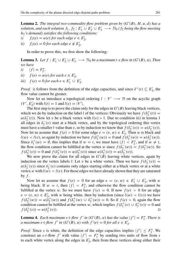
First observe that each white vertex v with |δ+1 (v)| = 2 already satisfies (1): v is aninner vertex of some ear Pi , and due to our construction δ−2 (v) and δ+2 (v) are separatedby the edges in E′1 incident to it (see fig. 6).

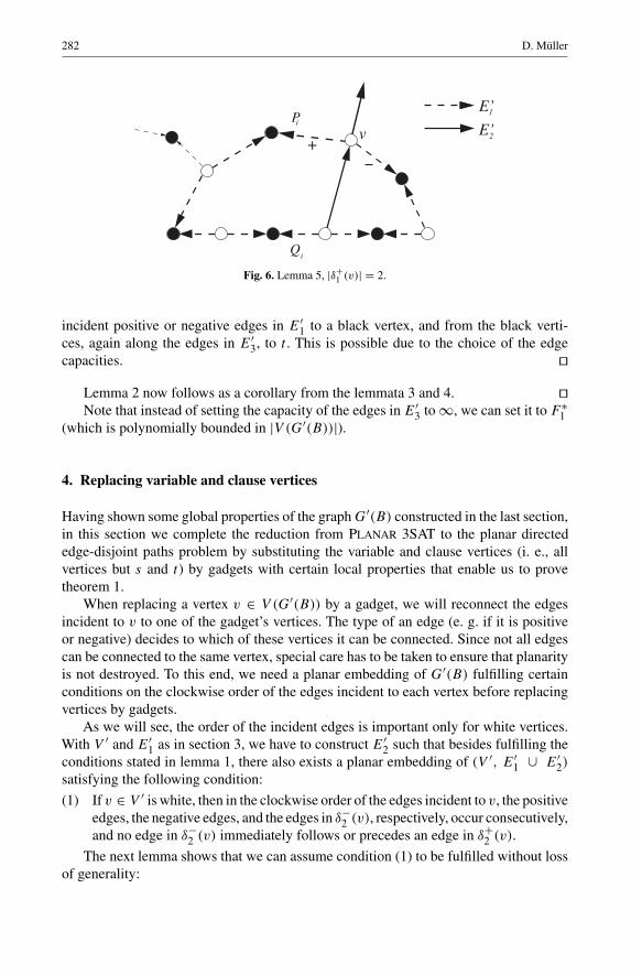
Now let v be a white vertex with |δ+1 (v)| = 3, i. e. the variable corresponding to v

occurs in three clauses c1, c2 and c3. Then v is an inner vertex of some ear Pi and an endvertex of another ear Pj with j > i. W. l. o. g. let c1, c3 ∈ Pi , c2 ∈ Pj and c3 ∈ Qj .Then between the edges (v, c1) and (v, c3) there lie some edges (at least one) in δ−2 (v),and the remaining edges in δ−2 (v) lie between (v, c2) and (v, c3). Let us denote the firstset of edges by Av,i and the second one by Av,j , so |Av,i | ≥ 1 and δ−2 (v) = Av,i ∪Av,j .The unique edge e+ ∈ δ+2 (v) must lie between (v, c1) and (v, c2), and there are no otheredges incident to v. See fig. 7 for an illustration of this situation.

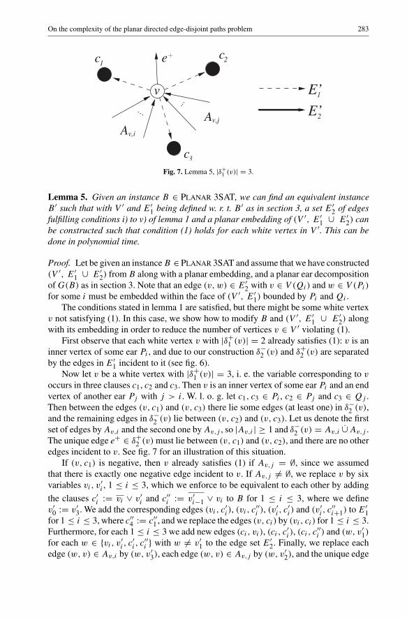
If (v, c1) is negative, then v already satisfies (1) if Av,j = ∅, since we assumedthat there is exactly one negative edge incident to v. If Av,j �= ∅, we replace v by sixvariables vi, v

′i , 1 ≤ i ≤ 3, which we enforce to be equivalent to each other by adding

the clauses c′i := vi ∨ v′i and c′′i := v′i−1 ∨ vi to B for 1 ≤ i ≤ 3, where we definev′0 := v′3. We add the corresponding edges (vi, c

′i ), (vi, c

′′i ), (v′i , c

′i ) and (v′i , c

′′i+1) to E′1

for 1 ≤ i ≤ 3, where c′′4 := c′′1 , and we replace the edges (v, ci) by (vi, ci) for 1 ≤ i ≤ 3.Furthermore, for each 1 ≤ i ≤ 3 we add new edges (ci, vi), (ci, c

′i ), (ci, c

′′i ) and (w, v′1)

for each w ∈ {vi, v′i , c′i , c′′i } with w �= v′1 to the edge set E′2. Finally, we replace each

edge (w, v) ∈ Av,i by (w, v′3), each edge (w, v) ∈ Av,j by (w, v′2), and the unique edge

284 D. Müller

Fig. 8. Lemma 5: Replacing v if |δ+1 (v)| = 3, (v, c1) is negative and Av,j �= ∅. Positive and negative edgesare marked by “+” and “−”, respectively.

(v, w) ∈ E′2 by (v′1, w). Since Av,j may be empty, we add an additional edge (c2, v′2)

to E′2 to ensure that v′2 can be reached from t (observe that c2 was reachable from t bycondition i) of lemma 1, and replacing v as described did not change this).

It is easy to see that planarity is preserved and that the planar embedding can bechosen such that the new white vertices satisfy condition (1) and for each of the otherwhite vertices, the clockwise order of the edges incident to it remains unchanged (seefig. 8).

So it remains to be verified that the conditions stated in lemma 1 remain fulfilled.We have already seen this for condition iv), and it is easy to check that also iii) and v)are satisfied. Condition i) still holds since s can be reached from v′1 in (V ′, E′2), andcondition ii) also continues to hold since (V ′, E′2) remains acyclic: It was acyclic before

replacing v, so also (V ′,←−E′1 ∪ E′2) was acyclic, where

←−E′1 := {(b, a) : (a, b) ∈ E′1}.

This is because←−E′1 contains only edges starting at a black and ending at a white vertex,

so a directed cycle must contain black and white vertices. But this is impossible sincethere is no edge starting at a white and ending at a black vertex. So the edges (ci, vi),(ci, c

′i ), (ci, c

′′i ) can be added to E′2 without introducing a cycle, for 1 ≤ i ≤ 3, as well

as (c2, v′2). It is easy to see that neither the new edges added to E′2 ending at v′1 can

introduce a cycle. So all conditions stated in lemma 1 continue to hold, and we havereduced the number of vertices violating condition (1) by one.

On the complexity of the planar directed edge-disjoint paths problem 285

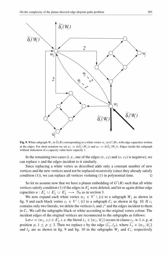
Fig. 9. White subgraph Wj in G(B) corresponding to a white vertex wj in G′(B), with edge capacities writtenat the edges. For short notation we set u2 := u(δ−2 (Wj )) and u3 := u(δ−3 (Wj )). Edges inside the subgraphwithout indication of a capacity value have capacity 1.

In the remaining two cases (i. e., one of the edges (v, c2) and (v, c3) is negative), wecan replace v and the edges incident to it similarly.

Since replacing a white vertex as described adds only a constant number of newvertices and the new vertices need not be replaced recursively (since they already satisfycondition (1)), we can replace all vertices violating (1) in polynomial time. �

So let us assume now that we have a planar embedding of G′(B) such that all whitevertices satisfy condition (1) if the edges in E′3 were deleted, and let us again define edgecapacities u : E′1 ∪ E′2 ∪ E′3 −→ N0 as in section 3.

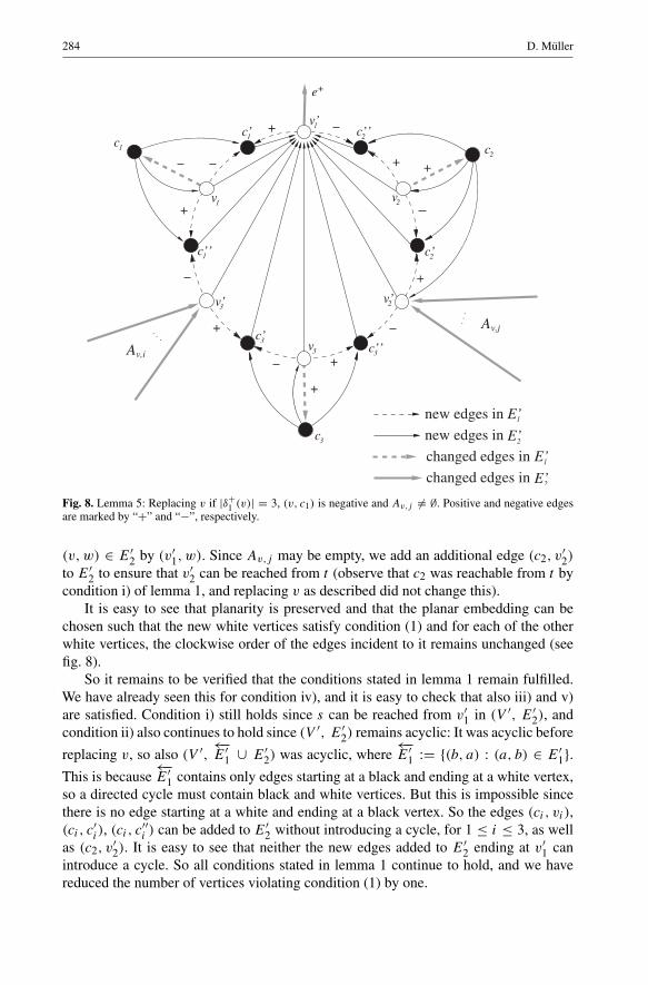
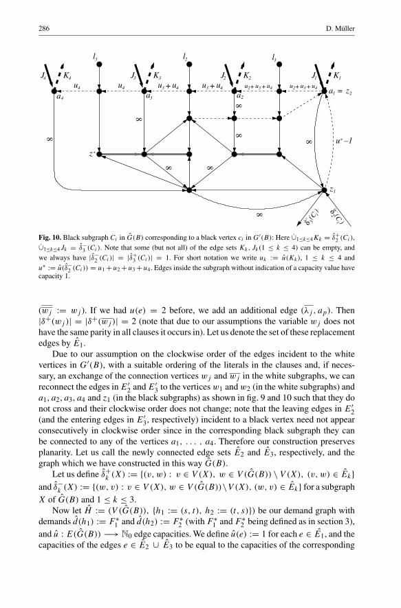
We now expand each white vertex wj ∈ V ′ \ {s} to a subgraph Wj as shown infig. 9 and each black vertex ci ∈ V ′ \ {t} to a subgraph Ci as shown in fig. 10. If ci

contains only two literals, we delete the vertices l3 and z∗ and the edges incident to themin Ci . We call the subgraphs black or white according to the original vertex colour. Theincident edges of the original vertices are reconnected to the subgraphs as follows:

Let e = (wj , ci) ∈ E′1, i. e. the literal λj ∈ {wj , wj } occurs in clause ci , w. l. o. g. atposition p, 1 ≤ p ≤ 3. Then we replace e by the edge (λj , lp), where λj ∈ {wj , wj }and lp are as shown in fig. 9 and fig. 10 in the subgraphs Wj and Ci , respectively

286 D. Müller

+ + + + ++

l3 l2 l1

a2

z1

z21a =

*z

u3 4ua4

u3

88

8

8 8

8

8

8

a3

u4 u4

u –1

u u u u u u2 3u4 4 2 3 4

K4J4 J3 K3 J2 K2 J1 K1

C)

C)

3i

i2

*

δ

δ

( (

Fig. 10. Black subgraph Ci in G(B) corresponding to a black vertex ci in G′(B): Here ∪1≤k≤4Kk = δ+2 (Ci),∪1≤k≤4Jk = δ−3 (Ci). Note that some (but not all) of the edge sets Kk, Jk(1 ≤ k ≤ 4) can be empty, andwe always have |δ−2 (Ci)| = |δ+3 (Ci)| = 1. For short notation we write uk := u(Kk), 1 ≤ k ≤ 4 andu∗ := u(δ−2 (Ci)) = u1+u2+u3+u4. Edges inside the subgraph without indication of a capacity value havecapacity 1.

(wj := wj ). If we had u(e) = 2 before, we add an additional edge (λj , ap). Then|δ+(wj )| = |δ+(wj )| = 2 (note that due to our assumptions the variable wj does nothave the same parity in all clauses it occurs in). Let us denote the set of these replacementedges by E1.

Due to our assumption on the clockwise order of the edges incident to the whitevertices in G′(B), with a suitable ordering of the literals in the clauses and, if neces-sary, an exchange of the connection vertices wj and wj in the white subgraphs, we canreconnect the edges in E′2 and E′3 to the vertices w1 and w2 (in the white subgraphs) anda1, a2, a3, a4 and z1 (in the black subgraphs) as shown in fig. 9 and 10 such that they donot cross and their clockwise order does not change; note that the leaving edges in E′2(and the entering edges in E′3, respectively) incident to a black vertex need not appearconsecutively in clockwise order since in the corresponding black subgraph they canbe connected to any of the vertices a1, . . . , a4. Therefore our construction preservesplanarity. Let us call the newly connected edge sets E2 and E3, respectively, and thegraph which we have constructed in this way G(B).

Let us define δ+k (X) := {(v, w) : v ∈ V (X), w ∈ V (G(B)) \ V (X), (v, w) ∈ Ek}and δ−k (X) := {(w, v) : v ∈ V (X), w ∈ V (G(B))\V (X), (w, v) ∈ Ek} for a subgraph

X of G(B) and 1 ≤ k ≤ 3.Now let H := (V (G(B)), {h1 := (s, t), h2 := (t, s)}) be our demand graph with

demands d(h1) := F ∗1 and d(h2) := F ∗2 (with F ∗1 and F ∗2 being defined as in section 3),and u : E(G(B)) −→ N0 edge capacities. We define u(e) := 1 for each e ∈ E1, and thecapacities of the edges e ∈ E2 ∪ E3 to be equal to the capacities of the corresponding

On the complexity of the planar directed edge-disjoint paths problem 287

edges in E′2 ∪ E′3. Let the capacities of the edges within the black and white subgraphsbe as shown in fig. 9 and 10.

Assume that there is a solution (f1, f2) to the integral two-commodity-flow problem(G(B), H , u, d). The following lemma shows the structure of the flows f1 and f2 withinthe black and white subgraphs in this case:

Lemma 6. Let (f1, f2) be a solution to the integral two-commodity-flow problem(G(B), H , u, d). Then with the notation from fig. 9 in each white subgraph Wj thefollowing holds:

i) In Wj exactly u(δ−2 (Wj )) units of the flow f2 travel from w1 to w2, and wehave f2(δ

+2 (Wj )) = f2(δ

−2 (Wj )) = u(δ−2 (Wj )) and f2(δ(V (Wj )) \ (δ−2 (Wj ) ∪

δ+2 (Wj ))) = 0,

ii) either f1(δ+(wj )) = 2 and f1(δ

+(wj )) = 0 or vice versa.

Using the notation from fig. 10, for each black subgraph Ci the following holds:

iii) In Ci exactly u(δ−2 (Ci)) units of the flow f2 travel from z1 to z2, and f2(K1 ∪ K2 ∪K3 ∪ K4) = f2(δ

+2 (Ci)) = f2(δ

−2 (Ci)) = u(δ−2 (Ci)), f2(δ(V (Ci)) \ (δ−2 (Ci) ∪

δ+2 (Ci))) = 0, and f2(e) = u(e) for all dashed edges e in fig. 10.

(iv) f1(δ−(l1 ∪ l2 ∪ l3)) ≤ 2, if the clause ci corresponding to Ci contains three

literals and f1(δ−(l1 ∪ l2)) ≤ 1 if ci contains only two literals.

Proof. i) follows from the construction of the white subgraphs and lemma 2.ii) From i) it can be followed that f1(δ

+({wj })) = 0 or f1(δ+({wj })) = 0, since

the flow f2 makes at least one of the vertices wj and wj unreachable from w2. Soii) holds for all white subgraphs incident to s since there we have f1(δ

−3 (Wj )) =

u(δ−3 (Wj )), so u(δ+3 (Wj )) = u(δ−3 (Wj ))− 2 implies that either f1(δ+({wj }) = 2

or f1(δ+({wj })) = 2. Furthermore, f1(δ

+3 (Wj )) = u(δ+3 (Wj )), so by induction it

can be followed that ii) holds for all white subgraphs.iii) follows from the construction of the black subgraphs and lemma 2.iv) follows from iii) and the construction of the black subgraphs: At least one of the

grey edges in fig. 10 must carry one unit of the flow f2, but also the f1-flow enteringin l1, l2 and l3, respectively, has to pass one of the grey edges since the dashed edgesare saturated by the f2-flow.

� Since the construction that we have described can be done in polynomial time,

theorem 1 follows as a corollary from the following theorem:

Theorem 2. Let B be an instance of Planar 3SAT. Then there is a solution (f1, f2) tothe integral two-commodity-flow problem (G(B), H , u, d) constructed from B as aboveif and only if B is satisfiable.

Proof. Let B be satisfiable. Let ci be a clause of B, λj ∈ {wj , wj } a literal in ci , Ci theblack subgraph in G(B) corresponding to ci , and Wj the white subgraph correspondingto the variable wj . If λj = wj , there is an edge from the vertex wj in the white subgraphWj to the black subgraph Ci , and if λj = wj , there is an edge from wj to Ci .

288 D. Müller: On the complexity of the planar directed edge-disjoint paths problem

Now let be given an assignment of truth values to the variables such that B is sat-isfied. Then we can construct a solution (f1, f2) to (G(B), H , u, d) as follows: Weconstruct an f1-flow of value |f1| = F ∗1 such that for each white subgraph Wj we havef1(δ

−3 (Wj )) = u(δ−3 (Wj )) and f1(δ

+3 (Wj )) = u(δ+3 (Wj )) = u(δ−3 (Wj )) − 2. If the

variable wj is true, we set f1(δ+(wj )) = u(δ+(wj )) = 2 and f1(δ

+(wj )) = 0, andconversely if wj is false. On the remaining edges we set f1 such that we get an s-t-flowand f1(E2) = 0 (see lemma 4).

A suitable construction of the flow f1 within the subgraphs allows the constructionof a t-s-flow f2 with |f2| = F ∗2 such that f1 + f2 respects the capacities u: Since eachclause is satisfied, in each black subgraph Ci we have f1(δ

−(l1 ∪ l2 ∪ l3)) ≤ 2, orf1(δ

−(l1 ∪ l2)) ≤ 1, respectively, if the corresponding clause contains only two literals,so f1 can be constructed such that at least one of the grey edges remains usable for theflow f2 and u(δ−2 (Ci)) units of flow can be sent from z1 to z2.

Conversely, let be given a solution (f1, f2) to (G(B), H , u, d). We set wj := “true”if f1(δ

+(wj )) > 0, and wj := “false” otherwise. From ii) and iv) in lemma 6 it followsthat this truth asignment satisfies B: iv) implies that each clause is satisfied by the truthassignment, while ii) ensures that a variable is evaluated to the same value in each clauseit occurs in. �

5. Conclusion

We have shown that the directed edge-disjoint paths problem remains NP-complete evenwhen restricted to planar supply graphs and demand graphs consisting of two sets ofparallel edges.

It is an open question whether also the undirected version of the problem is NP-com-plete. Since the orientation of the edges in our construction is crucial, it seems that ourproof cannot be carried over to the undirected case.

Acknowledgements. I am grateful to the anonymous referees for carefully reading the manuscript and forgiving helpful comments and suggestions improving the presentation.

References

1. Even, S., Itai, A., Shamir, A.: On the complexity of timetable and multicommodity flow problems. SIAMJ. Comput. 5, 691–703 (1976)

2. Karp, R.M.: On the computational complexity of combinatorial problems. Networks 5, 45–68 (1975)3. Korach, E., Penn, M.: A fast algorithm for maximum integral two-commodity flow in planar graphs.

Discrete Appl. Math. 47, 77–83 (1993)4. Korte, B., Vygen, J.: Combinatorial Optimization: Theory and Algorithms. Springer, Berlin, 20005. Kramer, M.R., van Leeuwen, J.: The complexity of wire-routing and finding minimum area layouts for

arbitrary VLSI circuits. In: Preparata, F.P. (ed.) VLSI-Theory Advances in Computing Research, Volume2. JAI Press, Greenwich, Connecticut, 1984

6. Lichtenstein, D.: Planar formulae and their uses. SIAM J. Comput. 11, 329–343 (1982)7. Middendorf, M., Pfeiffer, F.: On the complexity of the disjoint paths problem. Combinatorica 13(1),

97–107 (1993)8. Schrijver, A.: Finding k disjoint paths in a directed planar graph. SIAM J. Comput. 23, 780–788 (1994)9. Schrijver, A.: Combinatorial Optimization: Polyhedra and Efficiency. Springer, Berlin, 2003

10. Sebo, A.: Integer plane multiflows with a fixed number of demands. J. Comb. Theory Ser. B 59, 163–171(1993)