Embed Size (px)
Citation preview
ON THE CONCEPT OF
SYNTHETIC FIBER REINFORCED THIN-WALLED CONCRETE PIPES
By
ARASH EMAMI SALEH
Presented to the Faculty of the Graduate School of
The University of Texas at Arlington in Partial Fulfillment
of the Requirements
for the Degree of
DOCTOR OF PHILOSOPHY
THE UNIVERSITY OF TEXAS AT ARLINGTON
AUGUST 2019

ii
Copyright © by ARASH EMAMI SALEH 2019
All Rights Reserved

iii
ACKNOWLEDGMENTS
I would like to express my sincere gratitude to my doctoral advisor, Professor Ali Abolmaali, for
his endless support and guidance during the course of my Ph.D. studies. It has been my great
pleasure and honor to have the opportunity to work with him. Without his motivation, knowledge
and valuable advice, this research would not have been successfully completed. In addition, my
warm appreciation is extended to my doctoral committee members, Professors Shih-Ho Chao, Bo
Wang and Suyun Ham for their time, guidance, and helpful suggestions.
I am also very grateful to my wife Dr. Neda Habibi Arejan for her endless love, support,
encouragement, motivation and most of all being my best friend.
Thanks to my colleagues and friends Dr. Mohammad Razavi, Dr. Himan Hojat Jalali, Dr. Yeonho
Park, Dr. Maziar Mahdavi, Dr. Masoud Gharemannejad, Dr. Mahnaz Mostafazadeh, Sina Abhaee,
Bassam Al-lami and Dr.Alireza Sayah.
Last, but not least, I wish to extend my utmost heartfelt appreciation to my family for their endless
love, encouragement and support.
July 17 ,2019
iv
ABSTRACT
ON THE CONCEPT OF
SYNTHETIC FIBER REINFORCED THIN-WALLED CONCRETE PIPES
Arash Emami Saleh, PhD
The University of Texas at Arlington, 2019
Supervising Professor: Ali Abolmaali
This research investigates the structural and industrial possibility to create a new type of concrete
pipes called synthetic fiber reinforced thin-walled concrete pipes, which would be lighter, cheaper,
and more durable than what is currently in use while still providing a pipe product much less
dependent upon installation conditions than the very flexible metal and plastic pipes in the
American market. The idea is to reduce the thickness and reinforcement of the current reinforced
concrete pipes to increase their deflection before failure and control the crack formation and width
by using synthetic fibers. The flexibility of these pipes will enable them to use the passive pressure
of surrounding soil and in turn, relieves the pipe of the burden of carrying the soil load through
moment and shear in the pipe wall and allows it to perform primarily under compressive stress in
the pipe wall. To fulfill the research goal two phases of experimental investigations was performed.
The first phase was to understand the behavior of synthetic fiber reinforced TWCPs in Industrial
scale pipe production using a common industrial concrete mix design. In this phase, 44 pipes were
created and TEB test was performed on all the pipes. deformation curve for all tested specimens
was extracted and the cracking behavior of the pipes with and without using synthetic fibers was
v
observed. The second phase was to perform experimental study on crack development in synthetic
fiber reinforced concrete specimens. In this phase, 12 beam specimens were created using ASTM
1609 recommendations. The beams were tested in two groups of six beams under three and four-
point bending test setup. Crack width was measured using two-dimensional digital image
correlation (DIC) method. Finite element models were created to develop material model for
synthetic fiber reinforced concrete which can mimic the results of the tests. During the numerical
study a reliable crack width measurement method was introduced using the distribution of plastic
tensile strain in FE model. The last phase of numerical study was to create soil pipe interaction
models to evaluate the behavior of the pipes and their crack widths under soil backfill. A
parametric study was performed which led to development of equations to find the amount of crack
width as well as the design graphs.
vi
CONTENTS
ACKNOWLEDGMENTS ............................................................................................................. iii
ABSTRACT ................................................................................................................................... iv
LIST OF FIGURES ....................................................................................................................... ix
LIST OF TABLES ........................................................................................................................ xv
CHAPTER 1. INTRODUCTION ................................................................................................... 1
1.1. Overview ................................................................................................................................. 1
1.2. Rigid and Flexible Pipes in Current Practice ........................................................................... 2
1.3. Thin-Walled Concrete Pipe (TWCP): A Semi-Rigid Pipe ...................................................... 3
1.4. Goals and objectives ................................................................................................................ 5
1.5. Outline of Dissertation............................................................................................................. 6
CHAPTER 2. LITERATURE REVIEW ........................................................................................ 7
2.1. Design of concrete pipes .......................................................................................................... 7
2.1.1. Indirect Design method ................................................................................................ 8
2.1.2. Direct Design method ................................................................................................. 18
2.2. Synthetic Fiber Reinforced Concrete (Syn-FRC) .................................................................. 22
2.3. Finite Element Analysis and material models ....................................................................... 26
2.3.1. Constitutive model for Concrete ................................................................................. 29
2.3.2. Constitutive model for soil ......................................................................................... 35
CHAPTER 3. EXPERIMENTAL INVESTIGATION TO DEVELOP SYNTHETIC FIBER
REINFORCED THIN-WALLED CONCRETE PIPES ............................................................... 40
3.1. Experimental program in industrial level .............................................................................. 40
3.1.1. Material ....................................................................................................................... 40
3.1.2. Pipe Production Methods and Equipment .................................................................. 41
3.1.3. TEB tests and observations......................................................................................... 44
3.1.4. Load deformation curves ............................................................................................ 51
vii
3.1.5. Observations on stiffness ............................................................................................ 58
3.1.6. Conclusions of the TWCP tests .................................................................................. 60
CHAPTER 4. EXPERIMENTAL PROCESS OF CRACK WIDTH MEASUREMENT ............ 62
4.1. Experimental program on crack measurement in SynFR specimens .................................... 62
4.1.1. Experimental methods for crack width measurement ................................................ 62
4.1.2. Details of experimental program ................................................................................ 66
4.1.3. Results of experiments and DIC crack measurement ................................................. 71
4.1.4. Conclusions of the crack width measurement tests .................................................... 81
CHAPTER 5. FINITE ELEMENT SIMULATIONS OF THE TESTS ....................................... 82
5.1. Development of FE models for bending specimens .............................................................. 82
5.1.1. Geometry and FE mesh .............................................................................................. 83
5.1.2. Material model ............................................................................................................ 85
5.1.3. Crack width measurement process, results and conclusion ........................................ 88
5.2. Development of FE models for Three-Edge Bearing (TEB) tests ......................................... 94
5.2.1. Geometry and FE mesh .............................................................................................. 94
5.2.2. Material model ............................................................................................................ 97
5.2.3. Results and conclusions .............................................................................................. 98
5.3. Summary and conclusions ................................................................................................... 101
CHAPTER 6. FINITE ELEMENT SIMULATIONS OF SOIL-PIPE INTERACTION AND
PARAMETRIC STUDY ............................................................................................................ 102
6.1. Geometry and FE mesh ....................................................................................................... 102
6.2. Staged loading and model change ....................................................................................... 105
6.3. Material model ..................................................................................................................... 107
6.4. Parameters of the model ...................................................................................................... 108
6.5. Crack width measurement method ...................................................................................... 110
viii
6.6. Results ................................................................................................................................. 113
6.6.1. Reinforced TWCPs ................................................................................................... 113
6.6.2. Unreinforced TWCPs ............................................................................................... 118
6.7. Regression analysis.............................................................................................................. 124
6.7.1. Regression analysis for reinforced TWCPs .............................................................. 125
6.7.2. Regression analysis for unreinforced TWCPs .......................................................... 130
CHAPTER 7. SUMMARY AND CONCLUSIONS .................................................................. 135
7.1. Summary .............................................................................................................................. 135
7.2. Conclusion remarks ............................................................................................................. 138
7.3. Suggested future studies ...................................................................................................... 139
APPENDIX A. GRAPHS OF CRACK WIDTH FOR REINFORCED TWCPs ....................... 141
APPENDIX B. GRAPHS OF CRACK WIDTH FOR UNREINFORCED TWCPs .................. 157
REFERENCES ........................................................................................................................... 173
ix
LIST OF FIGURES
Figure 1.1 Overview of the benefits and philosophy of the TWCP................................................ 5
Figure 2.1 Essential Features of Types of Installations [2] ............................................................ 9
Figure 2.2 TEB test setup.............................................................................................................. 11
Figure 2.3 Load-deformation process in TEB test ........................................................................ 11
Figure 2.4 Standard Trench/Embankment Installation [2] ........................................................... 13
Figure 2.5 Arching factor and earth pressure distribution on rigid pipes [2] ............................... 15
Figure 2.6 Time-dependent behavior of 24-in [17] ...................................................................... 23
Figure 2.7 (a) linear, (b) linear with cracking in R and (c) linear with cracking in R and in S. [18]
............................................................................................................................................... 24
Figure 2.8 comparison of toughness in steel fiber reinforced specimens with different volume
fraction [23] .................................................................................................................................. 26
Figure 2.9 deviatory plane for CDP yield function [42] ............................................................... 31
Figure 2.10 CDP yield Surface under Biaxial Stress [42] ............................................................ 32
Figure 2.11 Dilation Angle and Eccentricity in a meridian view of potential function [42] ........ 33
Figure 2.12 Plastic Potential Surface and Yield Surface in the Deviatory Plane [42] .................. 33
Figure 2.13 a) uniaxial tensile and b) compressive curves and damage parameter [42] ............. 34
Figure 2.14 Mohr-Coulomb failure criterion [44] ........................................................................ 36
Figure 2.14 Mohr-Coulomb failure criterion in deviatoric plane [44].......................................... 37
Figure 2.15 the family of potential flow function in meridian plane [44] .................................... 39
Figure 2.16 smooth-corner flow potential function using Menetrey-Willam in deviatoric plane
[44] ............................................................................................................................................... 39
Figure 3.1 Pipe production: (a) production setup, (b) roller-head (called packerhead) (c) steel
cage on the end-joint steel ring, (d) rotation of the roller head and (e) removal of the jacket. .... 41
Figure 3.2 Comparison between RCP and TW pipe (ID: 1520mm=60in.) .................................. 44
Figure 3.3 (a) Three edge bearing test setup and (b) conceptual design philosophy of RCP and
FRCP ............................................................................................................................................. 45
Figure 3.4 Parallel Plate Test ........................................................................................................ 46
Figure 3.5 Comparison the crack distribution: 1370 mm (54 in.) and 1520 mm (60 in.) ............. 47
Figure 3.6 Crack development of TW pipes: 910 mm (36in.) and 3050 mm (120 in.) ................ 48
Figure 3.7 Comparison of circumferential cracks in FRCP (w/o a cage) and TW pipes (w/ a cage)
............................................................................................................................................... 49
Figure 3.8 Crack comparison of 3050 mm (120 in.) TW pipes. ................................................... 50
Figure 3.9 Load-deflection curve for (a) TWCP 30 in. (760 mm), (b) TWCP 36 in. (910 mm) .. 52
x
Figure 3.10 Load-deflection curve for (a) TWCP 54 in. (1370 mm), (b) TWCP 72in. (1830 mm) .
............................................................................................................................................... 53
Figure 3.11 Load-deflection curve for (a) TWCP 84 in. (2130 mm), (b) TWCP 120in. (3050 mm)
............................................................................................................................................... 54
Figure 3.12 Load-deflection curves of TW pipes (760 to 3050 mm): (𝐷𝑡 × 𝐴𝑠) ......................... 57
Figure 3.13 Load-deflection curves of pipes (3050mm=120 in.) (𝐷𝑡 × 𝐴𝑠) ................................ 57
Figure 3.14 Comparison of pipe stiffness between flexible and thin walled pipes ...................... 59
Figure 4.1 graduated scale (cracks’ comparator) .......................................................................... 62
Figure 4.2 Clip Gauge crack measurement ................................................................................... 63
Figure 4.3 setup for two-dimensional DIC crack measurement [48]............................................ 64
Figure 4.4 Reference Image: The yellow squares are the subsets ................................................ 65
Figure 4.5 Schematic scheme of Reference Subset and Deformed Subset to find the deformation
at P [48] ......................................................................................................................................... 65
Figure 4.6 Schematic View of three-point bending test setup based on RILEM TC 162-TDF [50]
............................................................................................................................................... 67
Figure 4.7 the rectangular jig to obtain the net deflection ............................................................ 67
Figure 4.8 Three-Point Bending Test Setup covered by gray pattern for DIC method ................ 68
Figure 4.9 four-point bending test setup as per ASTM C78-10 [52] ............................................ 68
Figure 4.10 LVDT and jig arrangement to measure the mid-span deflection four-point bending
test ............................................................................................................................................... 69
Figure 4.11 Test Setup for 4-Point Bending Test ......................................................................... 69
Figure 4.12 Clip Gauge (UB-5A) ................................................................................................. 70
Figure 4.13 development of random gray pattern for DIC ........................................................... 70
Figure 4.14 the setting of the camera for DIC process ................................................................. 71
Figure 4.15 Load - Deflection curves of three-Point bending test for 8PCY of fibers (VF=0.54%)
............................................................................................................................................... 71
Figure 4.16 Load - Deflection curves of three-Point bending test for 16PCY of fibers
(VF=1.04%) .................................................................................................................................. 72
Figure 4.17 Load - Deflection curves of four-Point bending test for 8PCY of fibers (VF=1.04%) .
............................................................................................................................................... 72
Figure 4.18 Load - Deflection curves of four-Point bending test for 16PCY of fibers (VF=1.04%)
............................................................................................................................................... 73
Figure 4.19 the quality control for the region of interest in DIC method using 2D GOM Correlate
software ......................................................................................................................................... 74
Figure 4.20 Deformation Field at the Onset of Cracking for one of three-Point Bending Tests .. 74
xi
Figure 4.21 Horizontal Displacement of the Points across the Crack Surface ............................. 75
Figure 4.22 Comparison of crack width measurement with different methods for 8PCY specimen
(VF=0.54%) .................................................................................................................................. 76
Figure 4.23 crack width measurement: comparison between ruler and DIC results. ................... 76
Figure 4.24 Crack Propagation in three-Point Bending Test of VF=0.54%: (a) Test 1 (b) Test 2
(c) Test 3 ....................................................................................................................................... 77
Figure 4.25 Crack Propagation in three-Point Bending Test of VF=1.04%: (a) Test 1 (b) Test 2
(c) Test 3 ....................................................................................................................................... 77
Figure 4.26 Load-CMOD for three-point bending test 8PCY specimens – VF=0.54% ............... 78
Figure 4.27 Load-CMOD for three-point bending test 16PCY specimens – VF=1.04% ............. 78
Figure 4.28 Crack Propagation in four-Point Bending Test of VF=0.54%: (a) Test 1 (b) Test 2 (c)
Test 3 ............................................................................................................................................. 79
Figure 4.29 Crack Propagation in four-Point Bending Test of VF=1.04%: (a) Test 1 (b) Test 2 (c)
Test 3 ............................................................................................................................................. 79
Figure 4.30 Load-CMOD for four-point bending test 8PCY specimens – VF=0.54% ................ 80
Figure 4.31 Load-CMOD for four-point bending test 16PCY specimens – VF=1.04% .............. 80
Figure 5.1 Different phases of finite element simulations ............................................................ 82
Figure 5.2 Geometry Beam Models for three-point and four-point bending tests ........................ 83
Figure 5.3 Schematic of 8-noded linear brick element ................................................................. 84
Figure 5.4 Typical mesh configuration in notched beam model .................................................. 84
Figure 5.5 Typical mesh configuration in un-notched beam model ............................................. 85
Figure 5.6 uniaxial compressive behavior of the concrete ........................................................... 86
Figure 5.7 the effect of fibers on uniaxial tensile behavior of concrete [58] ................................ 86
Figure 5.8 Schematic stress-crack width curve of uniaxial tensile behavior for Syn-FRC .......... 87
Figure 5.9 Stress-crack width curve of uniaxial tensile behavior for Syn-FRC with different VFs.
............................................................................................................................................... 88
Figure 5.10 Experimental vs FEM Load- Deflection for three-Point Bending – Syn-FRC, VF=
0.54% ............................................................................................................................................ 89
Figure 5.12 Experimental vs FEM Load- Deflection for four-Point Bending – Syn-FRC, VF=
0.54% ............................................................................................................................................ 90
Figure 5.13 Experimental vs FEM Load- Deflection for four-Point Bending – Syn-FRC, VF=
1.04% ............................................................................................................................................ 90
Figure 5.14 Typical Plastic Strain Distribution in a three-Point Bending Model ......................... 91
Figure 5.15 Typical Plastic Strain Distribution in a three-Point Bending Model ......................... 91
xii
Figure 5.16 Typical horizontal displacement contour-Relative displacement of two points can be
considered as crack width ............................................................................................................. 91
Figure 5.17 Experimental vs FEM Load-CMOD for three-Point Bending – Syn-FRC, VF=
0.54% ............................................................................................................................................ 92
Figure 5.18 Experimental vs FEM Load-CMOD for three-Point Bending – Syn-FRC, VF=
1.04% ............................................................................................................................................ 92
Figure 5.19 Experimental vs FEM Load-CMOD for four-Point Bending – Syn-FRC, VF= 0.54%
............................................................................................................................................... 93
Figure 5.20 Experimental vs FEM Load-CMOD for four-Point Bending – Syn-FRC, VF= 1.04%
............................................................................................................................................... 93
Figure 5.21 Typical geometry of FE models for TEB tests .......................................................... 95
Figure 5.22 Typical FE mesh for TEB tests ................................................................................. 96
Figure 5.23 uniaxial tensile behavior of Syn-FRC in pipes .......................................................... 97
Figure 5.24 uniaxial stress-strain curve of steel reinforcement materials .................................... 98
Figure 5.25 Results of TEB test modeling for TW36 ................................................................... 99
Figure 5.26 Results of TEB test modeling for TW54 ................................................................... 99
Figure 5.27 Results of TEB test modeling for TW60 ................................................................... 99
Figure 5.28 Results of TEB test modeling for TW72 ................................................................. 100
Figure 5.29 Results of TEB test modeling for TW84 ................................................................. 100
Figure 5.30 Comparison of crack patterns in FE analysis and test for TW84 ............................ 100
Figure 6.1 the typical geometry of the soil-pipe interaction models .......................................... 103
Figure 6.2 (a) front, (b) right side, (c) bottom surfaces of the model to apply boundary conditions
............................................................................................................................................. 104
Figure 6.3 Loosely placed bedding under the pipe according to real installation details ........... 104
Figure 6.4 General FE mesh of the soil-pipe interaction models ............................................... 105
Figure 6.5 Step by Step increasing the backfill height ............................................................... 106
Figure 6.6 Example plastic tensile strain contours for a TWCP at final step of loading ............ 111
Figure 6.7 General two-dimensional view of an element in section of the pipe ........................ 111
Figure 6.8 Relative displacements of the nodes of inside pipe circumference ........................... 112
Figure 6.9 Relative displacements of the nodes of outside pipe circumference ......................... 112
Figure 6.10 crack width in reinforced TWCPs in different diameters by changing Hunch soil.
Height of soil: 4 ft ....................................................................................................................... 113
Figure 6.11 crack width in reinforced TWCPs in different diameters by changing Hunch soil.
Height of soil: 8 ft ....................................................................................................................... 114
xiii
Figure 6.12 crack width in reinforced TWCPs in different diameters by changing Hunch soil.
Height of soil: 12 ft ..................................................................................................................... 114
Figure 6.13 crack width in reinforced TWCPs in different diameters by changing Hunch soil.
Height of soil: 16 ft ..................................................................................................................... 115
Figure 6.14 crack width in reinforced TWCPs in different diameters by changing Hunch soil.
Height of soil: 20 ft ..................................................................................................................... 115
Figure 6.15 crack width in reinforced TWCPs in different diameters by changing Hunch soil.
Height of soil: 24 ft ..................................................................................................................... 116
Figure 6.16 crack width in reinforced TWCPs in different diameters by changing Hunch soil.
Height of soil: 28 ft ..................................................................................................................... 116
Figure 6.17 crack width in reinforced TWCPs in different diameters by changing Hunch soil.
Height of soil: 32 ft ..................................................................................................................... 117
Figure 6.18 crack width in reinforced TWCPs in different diameters by changing Hunch soil.
Height of soil: 36 ft ..................................................................................................................... 117
Figure 6.19 crack width in reinforced TWCPs in different diameters by changing Hunch soil.
Height of soil: 40 ft ..................................................................................................................... 118
Figure 6.20 crack width in unreinforced TWCPs in different diameters by changing Hunch soil.
Height of soil: 4 ft ....................................................................................................................... 119
Figure 6.21 crack width in unreinforced TWCPs in different diameters by changing Hunch soil.
Height of soil: 8 ft ....................................................................................................................... 119
Figure 6.22 crack width in unreinforced TWCPs in different diameters by changing Hunch soil.
Height of soil: 12 ft ..................................................................................................................... 120
Figure 6.23 crack width in unreinforced TWCPs in different diameters by changing Hunch soil.
Height of soil: 16 ft ..................................................................................................................... 120
Figure 6.24 crack width in unreinforced TWCPs in different diameters by changing Hunch soil.
Height of soil: 20 ft ..................................................................................................................... 121
Figure 6.25 crack width in unreinforced TWCPs in different diameters by changing Hunch soil.
Height of soil: 24 ft ..................................................................................................................... 121
Figure 6.26 crack width in unreinforced TWCPs in different diameters by changing Hunch soil.
Height of soil: 28 ft ..................................................................................................................... 122
Figure 6.27 crack width in unreinforced TWCPs in different diameters by changing Hunch soil.
Height of soil: 32 ft ..................................................................................................................... 122
Figure 6.28 crack width in unreinforced TWCPs in different diameters by changing Hunch soil.
Height of soil: 36 ft ..................................................................................................................... 123
Figure 6.29 crack width in unreinforced TWCPs in different diameters by changing Hunch soil.
Height of soil: 40 ft ..................................................................................................................... 123
xiv
Figure 6.30 Comparison between FEM and predicted crack width in logarithmic scale for
reinforced TWCPs ...................................................................................................................... 126
Figure 6.31 Comparison between FEM and predicted crack width using new equations in
logarithmic scale for reinforced TWCPs .................................................................................... 129
Figure 6.32 Comparison between FEM and predicted crack width using new equations for
reinforced TWCPs ...................................................................................................................... 129
Figure 6.33 Comparison between FEM and predicted crack width in logarithmic scale for
unreinforced TWCPs .................................................................................................................. 131
Figure 6.34 Comparison between FEM and predicted crack width using new equations in
logarithmic scale for unreinforced TWCPs ................................................................................ 133
Figure 6.35 Comparison between FEM and predicted crack width using new equations for
unreinforced TWCPs .................................................................................................................. 134
xv
LIST OF TABLES
Table 2.1 practical requirements for each type of installation [2] ................................................ 13
Table 2.2 Equivalent USCS and AASHTO Soil Classifications for SIDD Soil Designations [2] 14
Table 2.3 Bedding factors for the embankment condition [2]. ..................................................... 16
Table 2.4 Different classes in ASTM C76. ................................................................................... 17
Table 3.1 Mechanical and Geometric Properties of BASF Synthetic Fibers ............................... 40
Table 3.1 Details of SynFR-TWCP specimens for experimental program .................................. 43
Table 3-2 the results of TW pipes tests ......................................................................................... 55
Table 3.3 Minimum required stiffness for HDPE pipes at 5% deflection .................................... 59
(AASHTO M294-10) [46] ............................................................................................................ 59
Table 5.1 Plasticity Parameters for CDP model ........................................................................... 85
Table 5.2 parameters of uniaxial tensile behavior of Syn-FRC .................................................... 88
Table5.3 Geometry properties of simulated pipes ........................................................................ 95
Table5.4 parameters of uniaxial tensile curve .............................................................................. 97
Table 6.1 Mechanical properties of bedding ............................................................................... 107
Table 6.2 Mechanical properties of backfill ............................................................................... 107
Table 6.3 Mechanical properties of loosely placed bedding ....................................................... 107
Table 6.4 Mechanical properties of hunch .................................................................................. 108
Table 6.5 Essential parameters of parametric study ................................................................... 109
Table 6.6 Independent parameters of regression analysis .......................................................... 124
Table 6.7 ANOVA for training data -Reinforced TWCPs ......................................................... 125
Table 6.8 Coefficients of the model -Reinforced TWCPs .......................................................... 125
Table 6.9 ANOVA for training data -Reinforced TWCPs (𝐶𝑤𝑖 < 0.003 𝑖𝑛.) ........................... 126
Table 6.10 Coefficients of the model -Reinforced TWCPs (𝐶𝑤𝑖 < 0.003 𝑖𝑛.) ......................... 127
Table 6.11 ANOVA for training data -Reinforced TWCPs (𝐶𝑤𝑖 > 0.003 𝑖𝑛.) ......................... 128
Table 6.12 Coefficients of the model -Reinforced TWCPs (𝐶𝑤𝑖 > 0.003 𝑖𝑛.) ......................... 128
Table 6.13 ANOVA for training data -Unreinforced TWCPs .................................................... 130
Table 6.14 Coefficients of the model -Unreinforced TWCPs .................................................... 130
Table 6.15 ANOVA for training data -Unreinforced TWCPs (𝐶𝑤𝑖 < 0.01 𝑖𝑛.) ....................... 131
Table 6.16 Coefficients of the model -Unreinforced TWCPs (𝐶𝑤𝑖 < 0.01 𝑖𝑛.) ........................ 132
Table 6.17 ANOVA for training data -Unreinforced TWCPs (𝐶𝑤𝑖 > 0.01 𝑖𝑛.) ....................... 132
Table 6.18 Coefficients of the model - Unreinforced TWCPs (𝐶𝑤𝑖 > 0.01 𝑖𝑛.) ....................... 133
1
CHAPTER 1. INTRODUCTION
1.1.Overview
Sewer and water supply networks are one of the most important infrastructure systems, account
for approximately half of the investments in United States [1]. One of the key items in a reliable
infrastructure is the buried pipe system. Specific engineering requirements should be considered
during the design and installation process of the buried pipelines. These requirements vary
markedly with the rigidity or the stiffness of the material selected for the pipe, dimensions and the
shape of embedment and the mechanical properties of the embedment and bedding soil. The soil
surrounding the pipe not only induces load on the pipe but also in a soil-structure interaction
system, the pipe develops its full structural performance [2].
There are two general methods of design for the buried pipe systems considering the soil-pipe
structural interaction: that is, evaluating the pipe as a rigid pipe, or evaluating it as a flexible pipe.
Rigid and flexible pipes are distinguished by the deflection ratio or by the relative stiffness of the
pipe. Rigid pipe systems only rely on the active soil pressure, and primarily resist the loads on the
pipe by carrying moment and shear in the pipe wall and start showing signs of structural failure
before being vertically deflected up to 2 % of their inside diameter [2-3]. Flexible pipe systems
such as corrugated metal pipe (CMP), polyethylene pipe (PE) and PVC pipe carry load by
deflecting out into the soil to pick up additional passive soil pressure, which then results primarily
in compressive forces in the pipe wall. Due to their different structural behavior characteristics,
rigid and flexible pipes have different design criteria and installation method [4].
Reinforced concrete pipe (RCP) is a rigid pipe, which upon loading has a deflection level that is
too small to develop lateral pressure. The benefit of relying primarily on the pipe strength, which
is assured since the pipe is produced in a factory, is promoted by the concrete pipe industry.
2
Flexible pipes may sometimes be cheaper in cost but rely much more heavily on the contractor’s
ability to perform a well-quality installation in the field, which often doesn't have the same Quality
Assurance (QA) control comparing to the plant environment. The performance of pipe product is
determined by external strength in the case of rigid pipes and by normal stiffness in the case of
flexible pipes, which require different installation standards for bedding and backing.
1.2.Rigid and Flexible Pipes in Current Practice
Metal and Plastic are the pipe materials of choice for flexible pipe systems in the US. In order to
keep their cost to a minimum, the producers of these pipe materials utilize corrugated wall
structures to enhance the pipe stiffness while reducing material. A side effect of this is that these
pipe materials also tend to have less wall area than the solid wall pipe, which more commonly
utilized in the water distribution market. Additionally, even with the corrugated walls, these pipe
materials have very low pipe stiffness. They can be as low as 105 kpa (15 psi) for a 1524 mm (60
in.) plastic pipe [5-6]. Most flexible pipe standards allow up to 5 % deflection. Deflection is
limited to 2 % if the flexible pipe has a rigid lining and coating and 3 % for a rigid lining and
flexible coating [7]. Specifiers call these pipes "flexible". However, they truly are very flexible
pipes and engineers and contractors have come to accept the installation risks that come with such
very flexible pipe. As noted previously, flexible pipe deflects into the surrounding soil and
develops primarily compressive stresses. Utilizing corrugated (or profile walls) allows plastic and
metal pipe producers to reduce their wall area. However, the thin profile sections are susceptible
to local buckling within their profile as well as global buckling of the wall while under
compression.
3
Concrete pipe represents the predominant pipe material used for rigid pipe systems in the storm
sewer market in the US. Concrete pipe is very durable and utilizes design methods that have been
in place for decades to design a pipe product that provides a large portion of the soil-structure on
its own. However, concrete pipe is brittle in comparison to metal and plastic pipes and can
experience only minute deformation in the field before it cracks. While concrete is expected to
crack, and cracking within service load limits is acceptable, for a standard wall concrete pipe to
develop passive soil pressure from the surrounding soil, it would need to deflect to an extent that
develops crack widths beyond allowable. Such large cracks in turn have the potential to allow
corrosion of the reinforcing steel should water and enough oxygen be present in the line. Thus,
American standards limit the allowable crack width in a buried concrete pipe to 0.25 mm (0.01
in.) for the service load condition.
1.3.Thin-Walled Concrete Pipe (TWCP): A Semi-Rigid Pipe
Research has been begun at the University of Texas at Arlington to develop concrete pipes that
would be lighter, cheaper, and more durable than what is currently in use, while still providing a
pipe product much less dependent upon installation conditions than the very flexible metal and
plastic pipes in the American market. Using Synthetic fibers in concrete mix design can improve
the behavior of concrete pipe and allows more deformation before failure. These pipes are TWCP,
semi-rigid pipes.
One of the benefits of using synthetic fibers is the effect they have on the cracking properties of
the concrete. Crack control in concrete is a function of bond between the reinforcement and
concrete, crack spacing and the amount of effective concrete area around the reinforcement. By
incorporating synthetic fibers in the mix that disperse throughout the concrete pipe wall in a
random fashion, the effective area of concrete around each fiber is much smaller than when a
4
standard circumferential steel reinforcing cage is used. Utilizing fibers in conjunction with
standard reinforcing steel result in several much smaller cracks as opposed to the few larger cracks
that occur with standard steel wire reinforcement.
Another issue that affects the crack width is the strain at the tensile surface of the concrete. The
larger the distance from the neutral axis of the wall to the wall surface, the larger the cracks at the
surface of the wall. If the concrete material in the pipe can be made flexible enough to allow for
some deflection of the pipe, then any potential loss of strength through thinning the wall can be
regained in the soil-structure through the additional passive soil support in the soil. Thus, a more
flexible concrete matrix with thinner wall thicknesses could be of maximum benefit for circular
buried structures.
The macro effect of this is that the concrete pipe can achieve significant levels of deflection without
developing cracks large enough to jeopardize the pipes durability. In other words, the pipe
becomes ductile (flexible). The further effect resulting from this flexibility is that the pipe deflects
sufficiently to produce passive pressure from the surrounding soil. This, in turn, relieves the pipe
of the burden of carrying the soil load through moment and shear in the pipe wall (as standard
reinforced concrete pipe does) and allows it to perform primarily under compressive stress in the
pipe wall. Concrete performs most suitably in compression, and unlike existing corrugate/profile
wall pipes, there are no local elements susceptible to local buckling. Thus, some of the most
significant concerns with flexible metal and plastic storm drainpipes are eliminated if a suitable
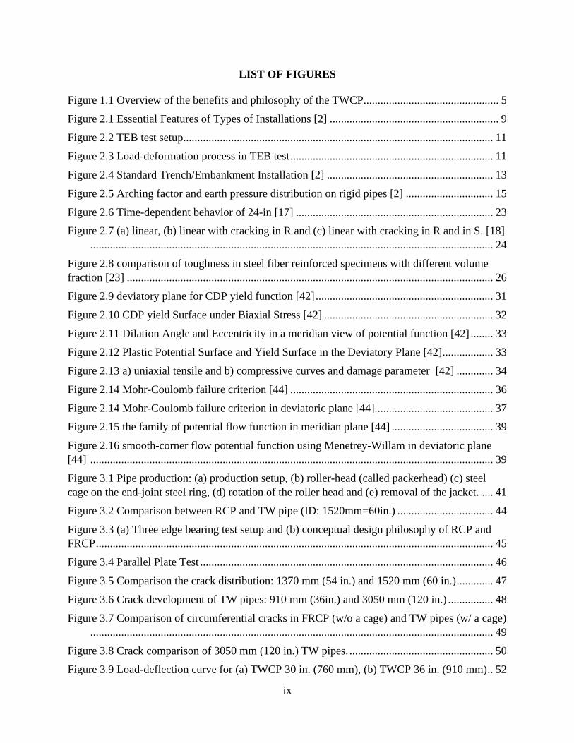
ductile concrete pipe can be developed. Figure 1.1 shows the overview of the benefits of the
TWCP.
5
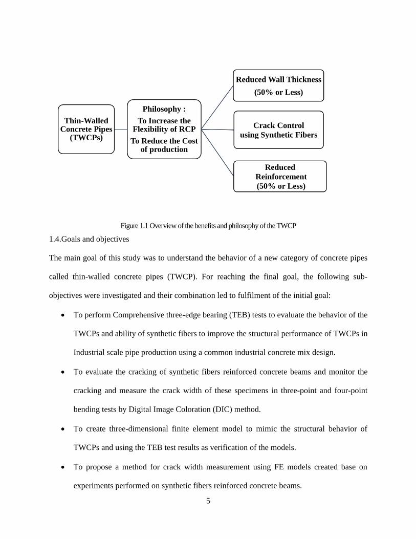
Figure 1.1 Overview of the benefits and philosophy of the TWCP
1.4.Goals and objectives
The main goal of this study was to understand the behavior of a new category of concrete pipes
called thin-walled concrete pipes (TWCP). For reaching the final goal, the following sub-
objectives were investigated and their combination led to fulfilment of the initial goal:
• To perform Comprehensive three-edge bearing (TEB) tests to evaluate the behavior of the
TWCPs and ability of synthetic fibers to improve the structural performance of TWCPs in
Industrial scale pipe production using a common industrial concrete mix design.
• To evaluate the cracking of synthetic fibers reinforced concrete beams and monitor the
cracking and measure the crack width of these specimens in three-point and four-point
bending tests by Digital Image Coloration (DIC) method.
• To create three-dimensional finite element model to mimic the structural behavior of
TWCPs and using the TEB test results as verification of the models.
• To propose a method for crack width measurement using FE models created base on
experiments performed on synthetic fibers reinforced concrete beams.
Thin-Walled Concrete Pipes
(TWCPs)
Philosophy :
To Increase the Flexibility of RCP
To Reduce the Cost of production
Reduced Wall Thickness
(50% or Less)
Crack Control
using Synthetic Fibers
Reduced
Reinforcement
(50% or Less)
6
• To develop soil-pipe interaction finite element models to evaluate the structural and
cracking behavior of proposed pipes and to perform a comprehensive parametric which
can lead to design method.
With the new category of concrete pipes, there would be about fifty percent reduction in the
thickness and reinforcement of current pipes. Synthetic fiber reinforced concrete as an innovative
material will be used in these pipes to control the cracks. The results of this research will let the
industries to manufacture TWCPs with a comprehensive understanding about their structural
behavior and engineering design process.
1.5.Outline of Dissertation
Chapter 2 presents a review of the current design procedure of the concrete pipes, the theoretical
background of FEM, the nonlinear behavior of the materials, details of contact and model changes
in FE procedure used in this research and the background of synthetic fibers reinforced concrete
materials and previous studies on these fibers. The experimental investigation on TWCPs is
presented in chapter 3 and a comprehensive study of different diameter of the concrete pipes,
focused on development of TWCPs in industrial level has been presented in this chapter. To
overcome the limitations of the concrete cracking due to deflection an experimental investigation
has been described in chapter 4 contains a detail investigation of crack width measurement of
synthetic fiber reinforced concrete specimens. Chapter 5 presents the development of FEM to
mimic the experimental results and verify the material models and the procedure of crack width
measurement. By using the verified models and procedure of crack width measurement, soil-pipe
interaction finite element models are presented in chapter 6. Finally, in chapter 6, the results of the
parametric study are used to find the design equations. Chapter 7 presents a summary of the results
and conclusions.
7
CHAPTER 2. LITERATURE REVIEW
2.1.Design of concrete pipes
Reinforced concrete pipes (RCPs) under the pressure of soil and the live loads behave as structural
elements in which the internal forces are developed. Similar to any other reinforced concrete
elements, the RCPs should be designed in a way that these internal forces can be developed inside
the pipe without causing any failure. The details of reinforcement and thickness based on design
process should be enough to provide sufficient strength for the pipes. There are two main design
methods based on which the RCPs can be designed: Direct Design method and Indirect Design
method.
• Indirect Design method utilizes an experimental process to evaluate the strength of the
pipes by using the results of a testing method called Three Edge Bearing (TEB) test
combined with a factor called bedding factor. In this method, the strength of the pipe in
TEB test is converted to the real field strength with presence of the soil by bedding factor.
The American Society for Testing and Materials (ASTM) has developed standard
specifications for precast concrete pipe. Each specification contains design, manufacturing
and testing criteria [2]. Based on the experimental nature of indirect design method and the
fact that this method is based on observed successful past installations, it is widely used in
ASTM standards for the design of RCPs.
• Direct Design method uses the ultimate internal forces coming from the structural analysis
of the pipe under external factored loads to find the area of the reinforcement and the
thickness of the pipe. This method uses the same process named limit state design of
reinforced concrete structures which is the well-known method of design based on ACI.
8
2.1.1.Indirect Design method
The first step in the design process is to find the loads applied to the structure. The amount of the
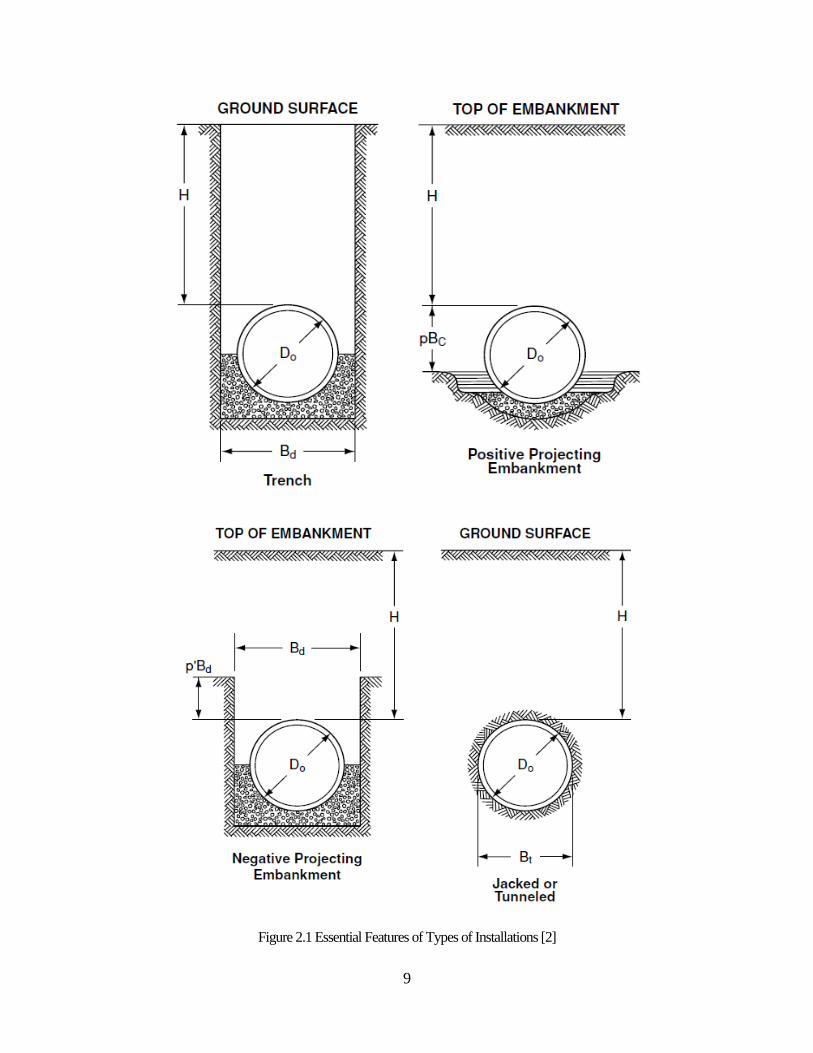
loads acting on the concrete pipe is largely dependent on the installation. There are three well-
known types of installation in pipe industry: Trench, Positive Projecting Embankment (PPE), and
Negative Projecting Embankment (NPE). Pipelines are also installed by jacking or tunneling
methods where deep installations are necessary or where conventional open excavation and
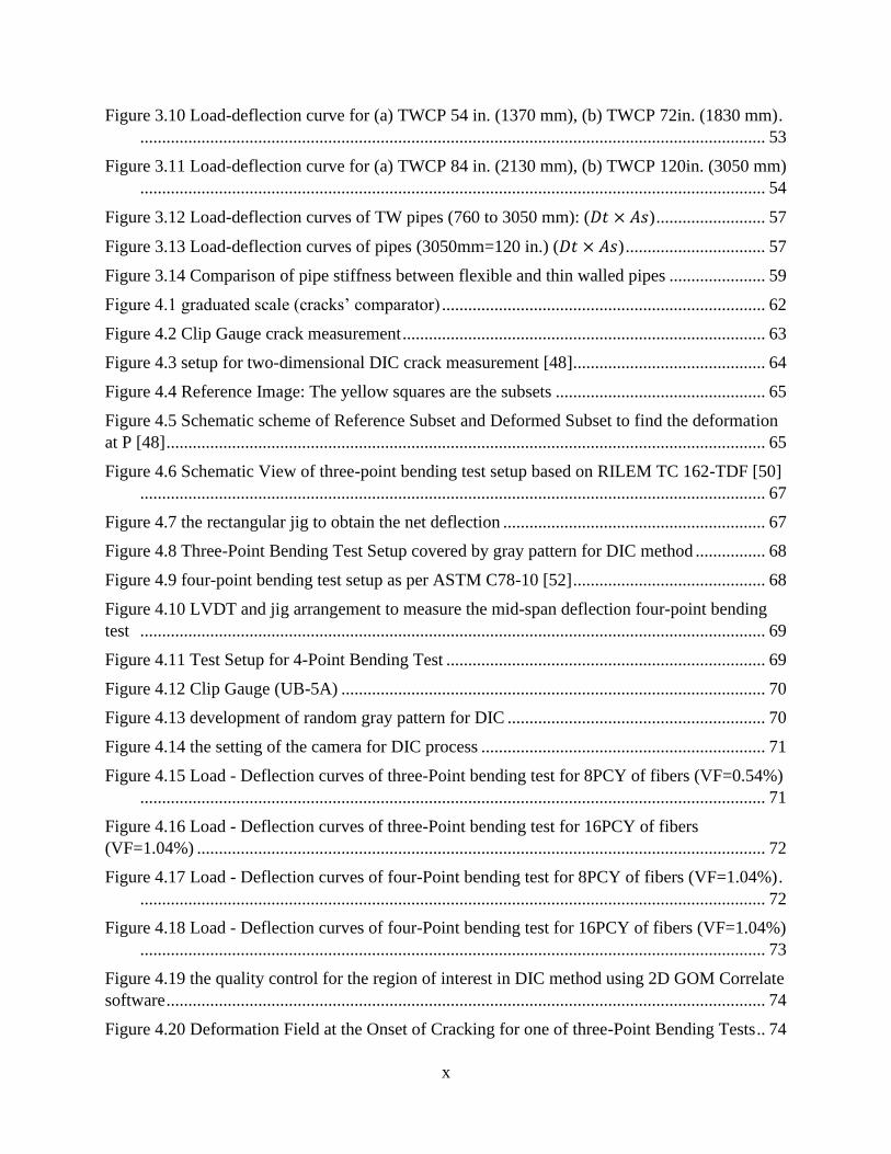
backfill methods may not be feasible [2]. Figure 2.1 shows the essential features of each of these
installations. In 1933 M.G.Spangler [8] stablished a theoretical method to find the soil pressure
acting on rigid pipes. In this method, three bedding configurations were supposed and the concept
of bedding factor was introduced for the first time. The concept of bedding factor is related to a
test of strength for the concrete pipes called Three Edge Bearing (TEB) test. The basic definition
of bedding factor is that it is the ratio of maximum moment in the three-edge bearing test to the
maximum moment in the buried condition as shown in Eq. 2-1, when the vertical loads under each
condition are equal [2]:
𝐵𝑓 =𝑀𝑇𝐸𝐵 𝑡𝑒𝑠𝑡
𝑀𝐵𝑢𝑟𝑖𝑒𝑑 Eq. 2-1
In which:
𝐵𝑓 : Bedding factor
𝑀𝑇𝐸𝐵 𝑡𝑒𝑠𝑡 : Maximum moment in pipe wall under TEB test load
𝑀𝐵𝑢𝑟𝑖𝑒𝑑 : Maximum moment in pipe wall under Buried condition
Spangler proposed that the bedding factor for a particular pipeline and, consequently, the
supporting strength of the buried pipe, is dependent on two installation characteristics [2]:
1. Width and quality of contact between the pipe and bedding.
2. Magnitude of lateral pressure and the portion of the vertical height of the pipe over which it acts.
9
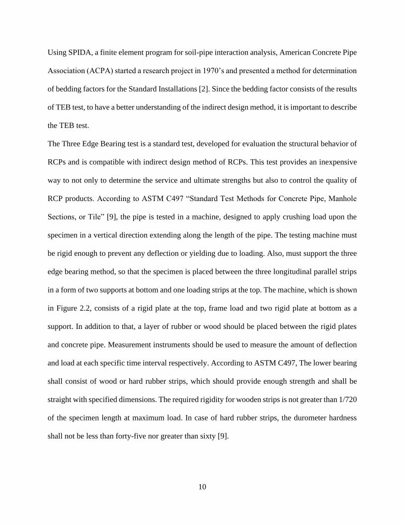
Figure 2.1 Essential Features of Types of Installations [2]
10
Using SPIDA, a finite element program for soil-pipe interaction analysis, American Concrete Pipe
Association (ACPA) started a research project in 1970’s and presented a method for determination
of bedding factors for the Standard Installations [2]. Since the bedding factor consists of the results
of TEB test, to have a better understanding of the indirect design method, it is important to describe
the TEB test.
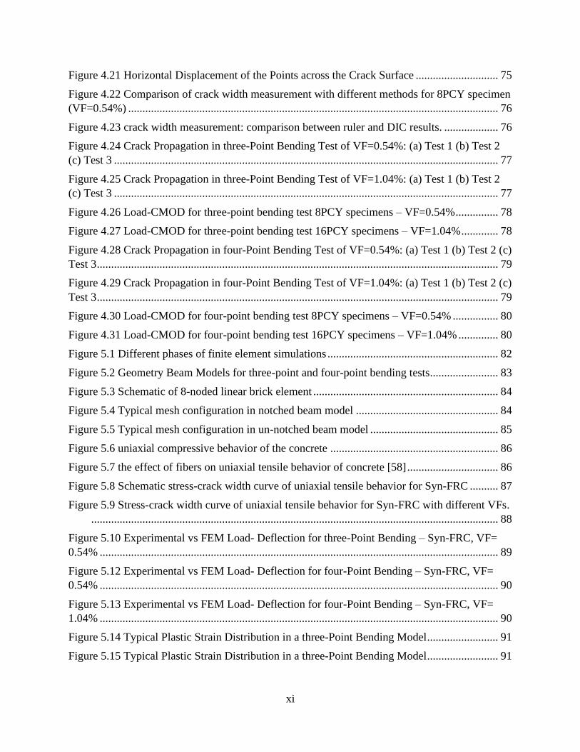
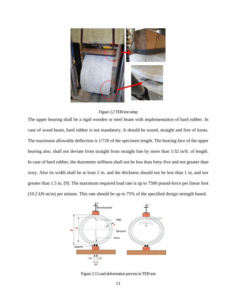
The Three Edge Bearing test is a standard test, developed for evaluation the structural behavior of
RCPs and is compatible with indirect design method of RCPs. This test provides an inexpensive
way to not only to determine the service and ultimate strengths but also to control the quality of
RCP products. According to ASTM C497 “Standard Test Methods for Concrete Pipe, Manhole
Sections, or Tile” [9], the pipe is tested in a machine, designed to apply crushing load upon the
specimen in a vertical direction extending along the length of the pipe. The testing machine must
be rigid enough to prevent any deflection or yielding due to loading. Also, must support the three
edge bearing method, so that the specimen is placed between the three longitudinal parallel strips
in a form of two supports at bottom and one loading strips at the top. The machine, which is shown
in Figure 2.2, consists of a rigid plate at the top, frame load and two rigid plate at bottom as a
support. In addition to that, a layer of rubber or wood should be placed between the rigid plates
and concrete pipe. Measurement instruments should be used to measure the amount of deflection
and load at each specific time interval respectively. According to ASTM C497, The lower bearing
shall consist of wood or hard rubber strips, which should provide enough strength and shall be
straight with specified dimensions. The required rigidity for wooden strips is not greater than 1/720
of the specimen length at maximum load. In case of hard rubber strips, the durometer hardness
shall not be less than forty-five nor greater than sixty [9].
11
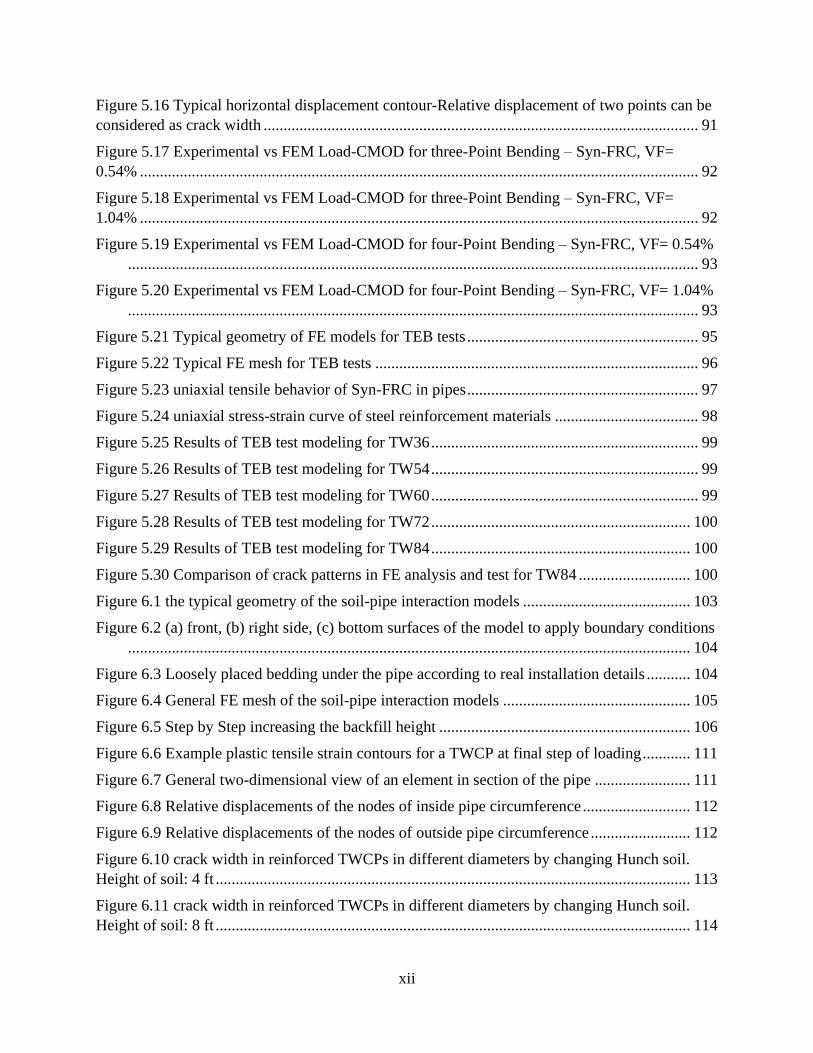
Figure 2.2 TEB test setup
The upper bearing shall be a rigid wooden or steel beam with implementation of hard rubber. In
case of wood beam, hard rubber is not mandatory. It should be sound, straight and free of knots.
The maximum allowable deflection is 1/720 of the specimen length. The bearing face of the upper
bearing also, shall not deviate from straight from straight line by more than 1/32 in/ft. of length.
In case of hard rubber, the durometer stiffness shall not be less than forty-five and not greater than
sixty. Also its width shall be at least 2 in. and the thickness should not be less than 1 in, and nor
greater than 1.5 in. [9]. The maximum required load rate is up to 7500 pound-force per linear foot
(10.2 kN-m/m) per minute. This rate should be up to 75% of the specified design strength based.
Figure 2.3 Load-deformation process in TEB test

12
The concept of bedding factor will help the designer to stablish Eq. 2-2 through which the needed
amount of moment in TEB test for the pipe will be determined. A factor of safety (F.S.) is needed
to convert the calculated parameters to real structural level:
(𝑀𝑇𝐸𝐵)𝑛𝑒𝑒𝑑𝑒𝑑 =𝑀𝐵𝑢𝑟𝑖𝑒𝑑
Bedding Factor× 𝐹. 𝑆. Eq. 2-2
Using the simple linear elastic structural analysis methods, it would be possible to re-wright the
Eq 2-2 based on the applied loads only:
(D − load)needed =WBuried
Modified Bedding Factor×F.S.
D Eq. 2-3
D − load =𝑇𝐸𝐵 𝑡𝑒𝑠𝑡 𝑡𝑜𝑡𝑎𝑙 𝑙𝑜𝑎𝑑
D × l Eq. 2-4
WBuried: The amount of load on the pipe in the field.
Modified Bedding Factor : Bedding factor considering the structural analysis modifications.
D and l: Inside diameter and length of the tested pipe respectively.
To determine the amount of load on the pipe in the field (WBuried) and corresponding bedding
factor, ACPA has developed four new Standard Installations. To find the bedding factor and
loadings, researcher focused on the positive projection embankment condition, which are the
worst-case vertical load conditions for pipe, and which provide conservative results for other
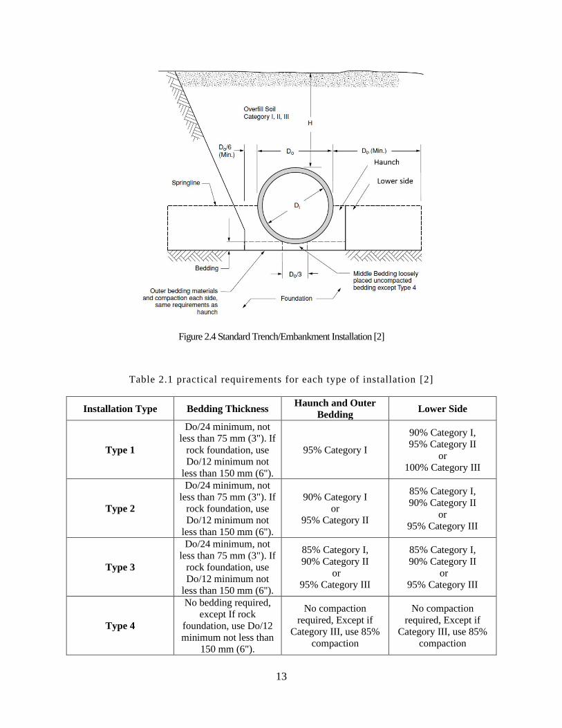
embankment and trench conditions [2]. Figure 2.4 shows the new standard installation system for
the trench and embankment. The installation types have arrange from high quality materials with
high compaction effort (Type 1) to low compaction effort and low quality material (Type 4). With
this new system of installation designer can choose to design a low strength pipe with a high quality
type 1 installation or a high strength pipe with low quality type 4 installation. Type 4 installation
can be used for the conditions where a little or no control is applied on installation process. Table
2.1 illustrates the practical requirements for each type of installation.
13
Figure 2.4 Standard Trench/Embankment Installation [2]
Table 2.1 practical requirements for each type of installation [2]
Installation Type Bedding Thickness Haunch and Outer
Bedding Lower Side
Type 1
Do/24 minimum, not
less than 75 mm (3"). If
rock foundation, use
Do/12 minimum not
less than 150 mm (6").
95% Category I
90% Category I,
95% Category II
or
100% Category III
Type 2
Do/24 minimum, not
less than 75 mm (3"). If
rock foundation, use
Do/12 minimum not
less than 150 mm (6").
90% Category I
or
95% Category II
85% Category I,
90% Category II
or
95% Category III
Type 3
Do/24 minimum, not
less than 75 mm (3"). If
rock foundation, use
Do/12 minimum not
less than 150 mm (6").
85% Category I,
90% Category II
or
95% Category III
85% Category I,
90% Category II
or
95% Category III
Type 4
No bedding required,
except If rock
foundation, use Do/12
minimum not less than
150 mm (6").
No compaction
required, Except if
Category III, use 85%
compaction
No compaction
required, Except if
Category III, use 85%
compaction

14
Generic soil types based on Unified Soil Classification System (USCS) and American Association
of State Highway and Transportation Officials (AASHTO) soil classifications is used in table 2.2
to relate different categories of Standard Installations Direct Design (SIDD) to the real practical
systems.
Table 2.2 Equivalent USCS and AASHTO Soil Classifications for SIDD Soil Designations [2]
Representative soil Types Percent Compaction
SIDD soil USCS AASHTO Standard
Proctor Modified Proctor
Gravelly Sand
(Category I) SW,SP,GW,GP A1,A3
100
95
90
85
80
61
95
90
85
80
75
59
Sandy Silt
(Category II)
GM,SM,ML,
Also GC,SC
With less than 20%
passing #200 sieve
A2,A4
100
95
90
85
80
49
95
90
85
80
75
46
Silty Clay
(Category III) CL,MH,GC,SC A5,A6
100
95
90
85
80
45
90
85
80
75
70
40
The type of installation affects the loads, carried by the rigid pipe. As a review of the load
calculation the soil load, applied to the pipe, in a PPE installation system is discussed here. In PPE
condition the soil the soil above the rigid pipe structure, will settle less than the soil along side of
the pipe. This process will impose additional load downward to the prism of soil directly above
the pipe. With the Standard Installations, this additional load will be considered by using a Vertical
Arching Factor, VAF, higher than 1.0. This factor is multiplied by the prism load, PL, (weight of
soil directly above the pipe) to give the total load of soil on the pipe [2]. Eq. 2-5 shows this
calculation:
15
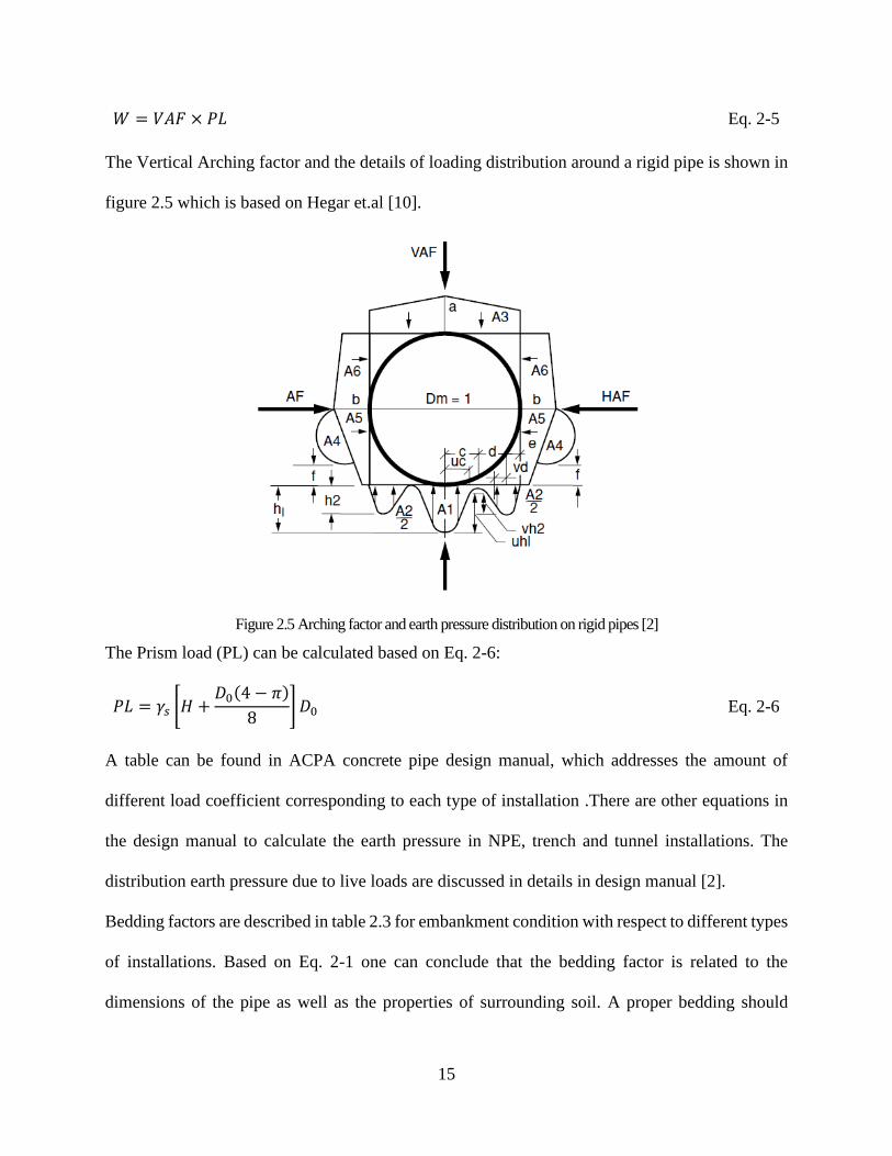
𝑊 = 𝑉𝐴𝐹 × 𝑃𝐿 Eq. 2-5
The Vertical Arching factor and the details of loading distribution around a rigid pipe is shown in
figure 2.5 which is based on Hegar et.al [10].
Figure 2.5 Arching factor and earth pressure distribution on rigid pipes [2]
The Prism load (PL) can be calculated based on Eq. 2-6:
𝑃𝐿 = 𝛾𝑠 [𝐻 +𝐷0(4 − 𝜋)
8]𝐷0 Eq. 2-6
A table can be found in ACPA concrete pipe design manual, which addresses the amount of
different load coefficient corresponding to each type of installation .There are other equations in
the design manual to calculate the earth pressure in NPE, trench and tunnel installations. The
distribution earth pressure due to live loads are discussed in details in design manual [2].
Bedding factors are described in table 2.3 for embankment condition with respect to different types
of installations. Based on Eq. 2-1 one can conclude that the bedding factor is related to the
dimensions of the pipe as well as the properties of surrounding soil. A proper bedding should
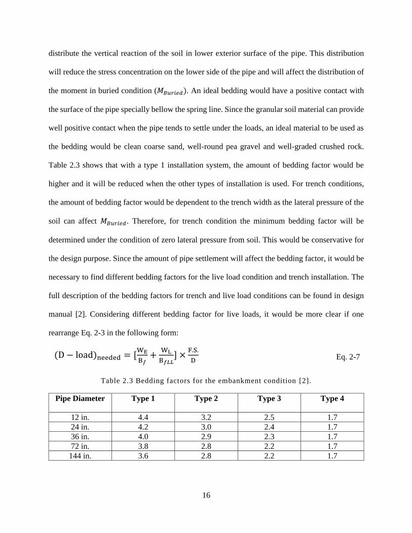
16
distribute the vertical reaction of the soil in lower exterior surface of the pipe. This distribution
will reduce the stress concentration on the lower side of the pipe and will affect the distribution of
the moment in buried condition (𝑀𝐵𝑢𝑟𝑖𝑒𝑑). An ideal bedding would have a positive contact with
the surface of the pipe specially bellow the spring line. Since the granular soil material can provide
well positive contact when the pipe tends to settle under the loads, an ideal material to be used as
the bedding would be clean coarse sand, well-round pea gravel and well-graded crushed rock.
Table 2.3 shows that with a type 1 installation system, the amount of bedding factor would be
higher and it will be reduced when the other types of installation is used. For trench conditions,
the amount of bedding factor would be dependent to the trench width as the lateral pressure of the
soil can affect 𝑀𝐵𝑢𝑟𝑖𝑒𝑑. Therefore, for trench condition the minimum bedding factor will be
determined under the condition of zero lateral pressure from soil. This would be conservative for
the design purpose. Since the amount of pipe settlement will affect the bedding factor, it would be
necessary to find different bedding factors for the live load condition and trench installation. The
full description of the bedding factors for trench and live load conditions can be found in design
manual [2]. Considering different bedding factor for live loads, it would be more clear if one
rearrange Eq. 2-3 in the following form:
(D − load)needed = [WE
B𝑓+
WL
B𝑓𝐿𝐿] ×
F.S.
D Eq. 2-7
Table 2.3 Bedding factors for the embankment condition [2].
Pipe Diameter Type 1 Type 2 Type 3 Type 4
12 in. 4.4 3.2 2.5 1.7
24 in. 4.2 3.0 2.4 1.7
36 in. 4.0 2.9 2.3 1.7
72 in. 3.8 2.8 2.2 1.7
144 in. 3.6 2.8 2.2 1.7
17
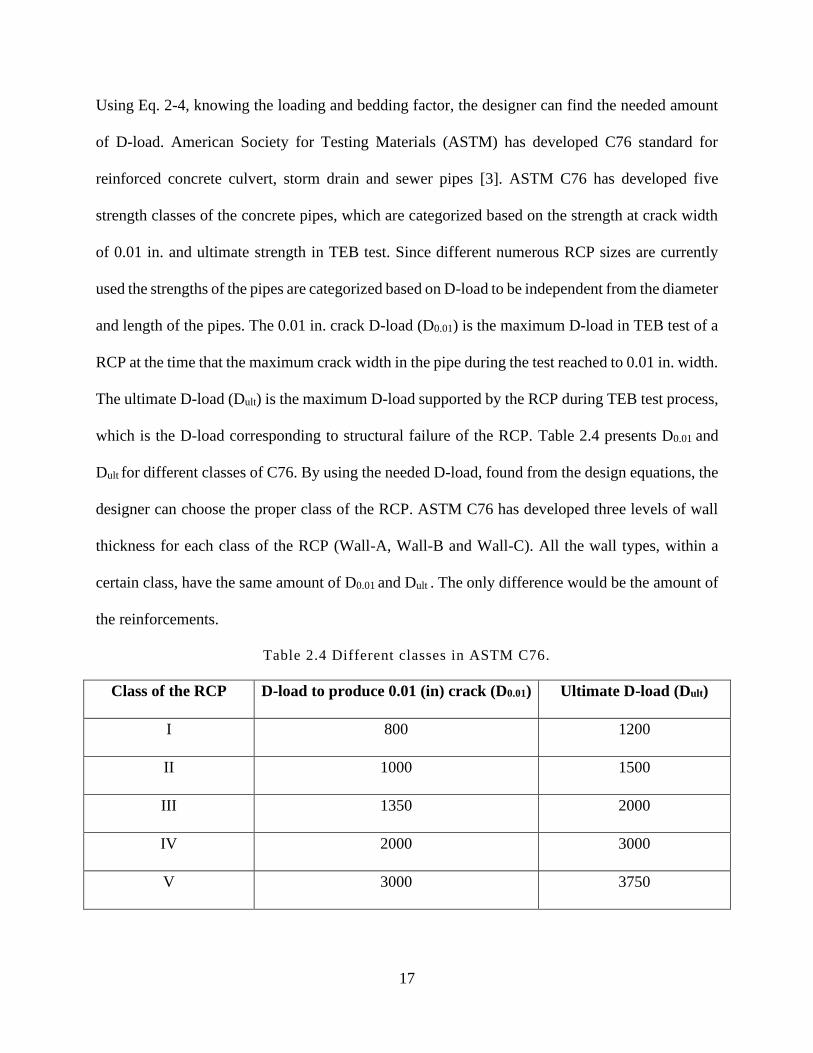
Using Eq. 2-4, knowing the loading and bedding factor, the designer can find the needed amount
of D-load. American Society for Testing Materials (ASTM) has developed C76 standard for
reinforced concrete culvert, storm drain and sewer pipes [3]. ASTM C76 has developed five
strength classes of the concrete pipes, which are categorized based on the strength at crack width
of 0.01 in. and ultimate strength in TEB test. Since different numerous RCP sizes are currently
used the strengths of the pipes are categorized based on D-load to be independent from the diameter
and length of the pipes. The 0.01 in. crack D-load (D0.01) is the maximum D-load in TEB test of a
RCP at the time that the maximum crack width in the pipe during the test reached to 0.01 in. width.
The ultimate D-load (Dult) is the maximum D-load supported by the RCP during TEB test process,
which is the D-load corresponding to structural failure of the RCP. Table 2.4 presents D0.01 and
Dult for different classes of C76. By using the needed D-load, found from the design equations, the
designer can choose the proper class of the RCP. ASTM C76 has developed three levels of wall
thickness for each class of the RCP (Wall-A, Wall-B and Wall-C). All the wall types, within a
certain class, have the same amount of D0.01 and Dult . The only difference would be the amount of
the reinforcements.
Table 2.4 Different classes in ASTM C76.
Class of the RCP D-load to produce 0.01 (in) crack (D0.01) Ultimate D-load (Dult)
I 800 1200
II 1000 1500
III 1350 2000
IV 2000 3000
V 3000 3750
18
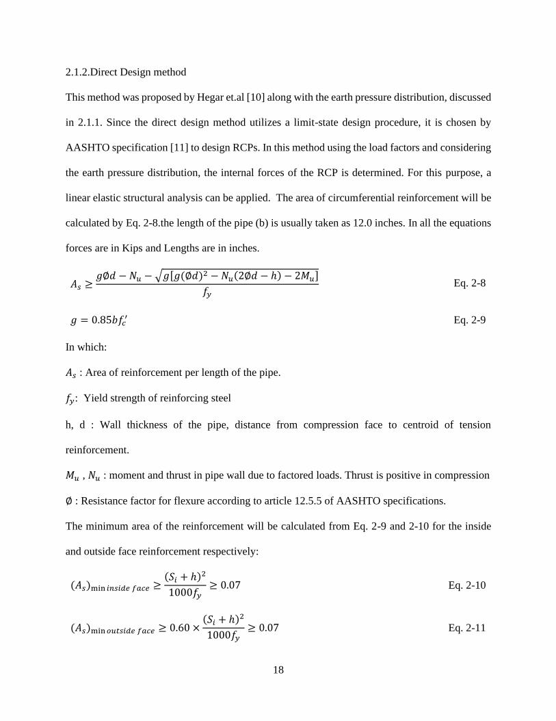
2.1.2.Direct Design method
This method was proposed by Hegar et.al [10] along with the earth pressure distribution, discussed
in 2.1.1. Since the direct design method utilizes a limit-state design procedure, it is chosen by
AASHTO specification [11] to design RCPs. In this method using the load factors and considering
the earth pressure distribution, the internal forces of the RCP is determined. For this purpose, a
linear elastic structural analysis can be applied. The area of circumferential reinforcement will be
calculated by Eq. 2-8.the length of the pipe (b) is usually taken as 12.0 inches. In all the equations
forces are in Kips and Lengths are in inches.
𝐴𝑠 ≥𝑔∅𝑑 − 𝑁𝑢 −√𝑔[𝑔(∅𝑑)2 − 𝑁𝑢(2∅𝑑 − ℎ) − 2𝑀𝑢]
𝑓𝑦 Eq. 2-8
𝑔 = 0.85𝑏𝑓𝑐′ Eq. 2-9
In which:
𝐴𝑠 : Area of reinforcement per length of the pipe.
𝑓𝑦: Yield strength of reinforcing steel
h, d : Wall thickness of the pipe, distance from compression face to centroid of tension
reinforcement.
𝑀𝑢 , 𝑁𝑢 : moment and thrust in pipe wall due to factored loads. Thrust is positive in compression
∅ : Resistance factor for flexure according to article 12.5.5 of AASHTO specifications.
The minimum area of the reinforcement will be calculated from Eq. 2-9 and 2-10 for the inside
and outside face reinforcement respectively:
(𝐴𝑠)min 𝑖𝑛𝑠𝑖𝑑𝑒 𝑓𝑎𝑐𝑒 ≥(𝑆𝑖 + ℎ)
2
1000𝑓𝑦≥ 0.07 Eq. 2-10
(𝐴𝑠)min𝑜𝑢𝑡𝑠𝑖𝑑𝑒 𝑓𝑎𝑐𝑒 ≥ 0.60 ×(𝑆𝑖 + ℎ)
2
1000𝑓𝑦≥ 0.07 Eq. 2-11

19
𝑆𝑖: Internal diameter of the pipe
In most cases, RCPs are designed without reinforcement. To control the crack in concrete because
of radial tension due to bending the AASHTO specification [10] considers a maximum area for
the reinforcement in tension based on Eq. 2-12:
(𝐴𝑠)𝑚𝑎𝑥 ≤0.506𝑟𝑠𝐹𝑟𝑝√𝑓𝑐′(𝑅∅)𝐹𝑟𝑡
𝑓𝑦 Eq. 2-12
𝑟𝑠 : Radius of inside reinforcement.
𝑅∅: Ratio of resistance factors of radial tension and moment according to article 12.5.5 of
AASHTO specifications.
𝐹𝑟𝑝 : 1.0 unless a higher value can be assigned based on the tests.
𝐹𝑟𝑡 :
• For 12.0 in. ≤ 𝑆𝑖 ≤ 72.0 in. : 𝐹𝑟𝑡 = 1 + 0.00833(72 − 𝑆𝑖)
• For 72.0 in. ≤ 𝑆𝑖 ≤ 144.0 in. : 𝐹𝑟𝑡 =(72−𝑆𝑖)
2
26000+ 0.8
• For 𝑆𝑖 ≥ 144.0 in. : 𝐹𝑟𝑡 = 0.8
For reinforcements in compression:
(𝐴𝑠)𝑚𝑎𝑥 ≤
(55𝑔′∅𝑑87 + 𝑓𝑦
) − 0.75𝑁𝑢
𝑓𝑦
Eq. 2-13
𝑔′ = 𝑏𝑓𝑐′[0.85 − 0.05(𝑓𝑐
′ − 4.0)] Eq. 2-14
0.85𝑏𝑓𝑐′ ≥ 𝑔′ ≥ 0.65𝑏𝑓𝑐
′ Eq. 2-15
In all the equations, the length of the pipe (b) is taken as 12.0 inches.
To control the crack width, direct design method utilizes a crack width factor (𝐹𝑐𝑟) which can be
determined as:
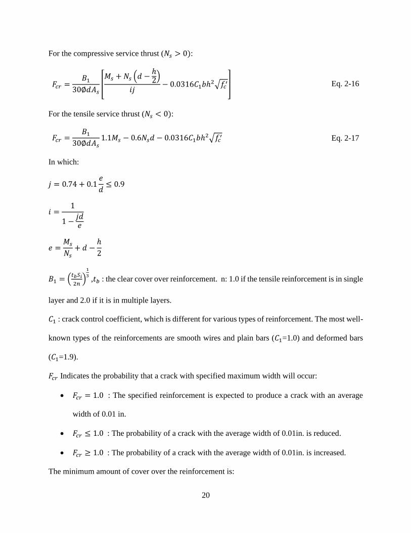
20
For the compressive service thrust (𝑁𝑠 > 0):
𝐹𝑐𝑟 =𝐵1
30∅𝑑𝐴𝑠[𝑀𝑠 + 𝑁𝑠 (𝑑 −
ℎ2)
𝑖𝑗− 0.0316𝐶1𝑏ℎ
2√𝑓𝑐′] Eq. 2-16
For the tensile service thrust (𝑁𝑠 < 0):
𝐹𝑐𝑟 =𝐵1
30∅𝑑𝐴𝑠1.1𝑀𝑠 − 0.6𝑁𝑠𝑑 − 0.0316𝐶1𝑏ℎ
2√𝑓𝑐′ Eq. 2-17
In which:
𝑗 = 0.74 + 0.1𝑒
𝑑≤ 0.9
𝑖 =1
1 −𝑗𝑑𝑒
𝑒 =𝑀𝑠
𝑁𝑠+ 𝑑 −
ℎ
2
𝐵1 = (𝑡𝑏𝑆𝑖
2𝑛)
1
3 ,𝑡𝑏 : the clear cover over reinforcement. n: 1.0 if the tensile reinforcement is in single
layer and 2.0 if it is in multiple layers.
𝐶1 : crack control coefficient, which is different for various types of reinforcement. The most well-
known types of the reinforcements are smooth wires and plain bars (𝐶1=1.0) and deformed bars
(𝐶1=1.9).
𝐹𝑐𝑟 Indicates the probability that a crack with specified maximum width will occur:
• 𝐹𝑐𝑟 = 1.0 : The specified reinforcement is expected to produce a crack with an average
width of 0.01 in.
• 𝐹𝑐𝑟 ≤ 1.0 : The probability of a crack with the average width of 0.01in. is reduced.
• 𝐹𝑐𝑟 ≥ 1.0 : The probability of a crack with the average width of 0.01in. is increased.
The minimum amount of cover over the reinforcement is:

21
• 0.75 in.: for the wall thickness less than 2.5 in.
• 1.0 in.: for the wall thickness more than 2.5 in.
Since it is very complicated in practice to put radial stirrups in RCPs, in most of the cases, RCPs
are design without using any radial stirrups. Eq. 2-18 presents Shear design equation for these
RCPs:
𝑉𝑟 = ∅𝑉𝑛 Eq. 2-18
𝑉𝑛 = 0.0316𝑏𝑑𝐹𝑣𝑝√𝑓𝑐′(1.1 + 63𝜌) (𝐹𝑑𝐹𝑛𝐹𝑐
) Eq. 2-19
𝜌 =𝐴𝑠
𝑏𝑑≤ 0.02
𝐹𝑑 = 0.8 +1.6
𝑑≤ 1.3 : For the RCPs with two cages of reinforcements of elliptical one.
For the compressive ultimate thrust (𝑁𝑢 > 0):
• 𝐹𝑛 = 1 +𝑁𝑢
24ℎ
For the tensile ultimate thrust (𝑁𝑢 < 0):
• 𝐹𝑛 = 1 +𝑁𝑢
6ℎ
𝐹𝑐 = 1 ±𝑑
2𝑟 In which, r is radius of the centerline of the concrete pipe wall. If the tension is inside
the pipe (crown and invert) the positive sign should be used and vice versa
𝐹𝑣𝑝 : A factor related to the process and material of the pipe. According to article 12.10.4.2.3 of
AASHTO specifications.
If the factored shear load (𝑉𝑢) is greater than 𝑉𝑟 the radial shear stirrups should be provided or the
thickness of the pipe should be increase to take the shear force.
22
2.2.Synthetic Fiber Reinforced Concrete (Syn-FRC)
Steel fibers have been used for a long time in concrete mixture to reduce the brittle nature of the
concrete due to tensile stresses. In some cases, researchers proved the ability of steel fibers to be
good replacements of reinforcements in concrete. The advantages of using steel fibers in concrete
to replace the reinforcement, have led the industry and researchers to develop other kind of fibers
with different materials. The most important shortcoming of steel fibers is their low resistance with
respect to corrosion. Also using steel fibers, it would be challenging to obtain a smooth surface of
the concrete and finishabilty have been always one of the problems. Considering these problems,
fibers created from nonmetallic materials can be good replacement of steel fibers. Various types
of synthetic materials such as glass, nylon, acrylic, carbon, polyester, polyethylene, and
polypropylene have been used as fibers in concrete. Researches on synthetic fibers proved that
they would enhance the toughness and impact resistance of concrete and control the crack widths
and shrinkage effects [12]-[16].
The effect of adding synthetic fibers to the mix design of concrete has been investigated by many
researches. Particularly, the possibility of developing the synthetic fiber reinforced concrete pipes
(Syn-FRCPs) investigated by Wilson and Abolmaali [12]. They evaluated the synthetic fibers as
an alternative reinforcement in concrete pipes. They compared the mechanical behavior of dry-
cast concrete specimens reinforced with steel and synthetic fibers considering different amount of
fiber dosage. Compressive strength and cracking strength were compared and the results
demonstrated that synthetic fibers increase the impact resistance and toughness of concrete .They
did the TEB test on the concrete pipes and concluded that the synthetic fibers can be a good
alternative for reinforcement and reduce crack width and plastic shrinkage seen in concrete pipes.
23
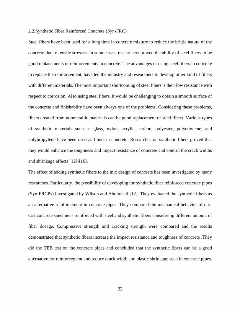
Park et al. [17] investigated the Time-Dependent Behavior of Syn-FRCPs. They tested the pipes
in a long-term loading condition both under a three-edge bearing test and in the real trench in field.
All buried pipes were pre-cracked until the first visible crack was observed. The pre-cracking was
done to evaluate the long-term performance of Syn-FRCPs in which fibers are engaged after
cracking. The strength, crack width and gradual change in vertical deformation is monitored during
the test. The total deflection of the Syn-FRCPs after 4200 hours was 2.83% and 1.61% of inside
diameter for 24 in. and 36 in. internal diameter of the pipes respectively. The addition of synthetic
fibers to the concrete mixtures of the pipes enhanced the load bearing capacity of the pipes. Figure
2.6 presents a graph of change of deflection versus time for the diameter of 24 in.
Figure 2.6 Time-dependent behavior of 24-in [17]
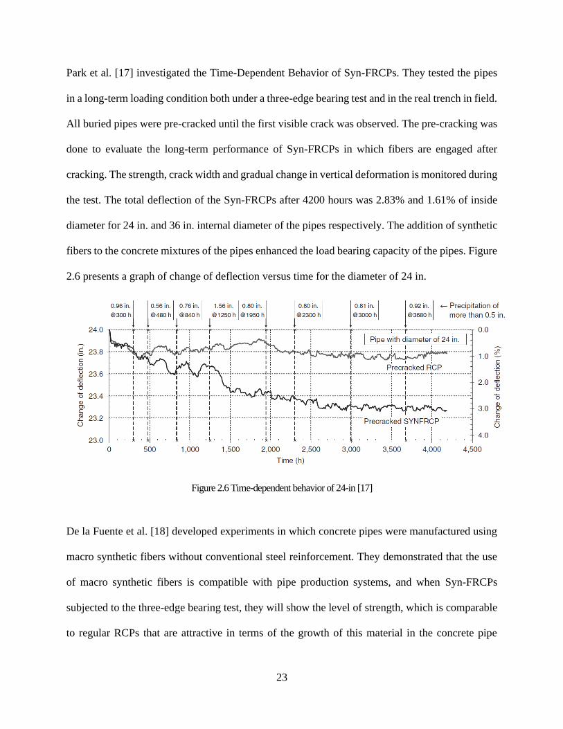
De la Fuente et al. [18] developed experiments in which concrete pipes were manufactured using
macro synthetic fibers without conventional steel reinforcement. They demonstrated that the use
of macro synthetic fibers is compatible with pipe production systems, and when Syn-FRCPs
subjected to the three-edge bearing test, they will show the level of strength, which is comparable
to regular RCPs that are attractive in terms of the growth of this material in the concrete pipe
24
industry. They also developed a Model for the Analysis of Pipes (MAPs) as a tool for the design
of Syn-FRCPs. Figure 2.7 shows the MAPs.
Figure 2.7 (a) linear, (b) linear with cracking in R and (c) linear with cracking in R and in S. [18]
Peyvandi et al. performed Comprehensive experimental investigations to evaluate the efficiency
of different synthetic fibers (aramid, R-glass, carbon, and polyvinyl alcohol (PVA)) at various
volume fractions. They realized that, at Industrial-scale, evaluation of concrete pipes indicates 30%
improvement in load-carrying capacity with introduction of PVA fibers. This improvement
enables industries to reduce welded wire fabric steel reinforcement layer in concrete pipes from
two to one. This will increasing the protective concrete cover thickness over steel and durability
of concrete pipes under the aggressive exposure conditions of sanitary sewers .The research
showed that by using fibers it would be possible to reduce the wall thickness of the of the pipes
and thus its overall weight , production, transportation and installation costs would be decreased
[19].
Mostafazadeh and Abolmaali performed a comprehensive experimental study on shear capacity of
Syn-FRCs. They considered two level of compressive strength for the concrete and used a dry-cast
and zero-slump mix [20]. The results of this experiments showed that the application of synthetic
25
fibers in concrete yielded to significant improvement in shear strength, shear toughness and
flexural strength of the concrete.
Roesler et al. conducted a study on fiber-reinforced slabs, with steel and synthetic fibers using two
level of volume fractions. The results showed that by using less than 1% volume fraction of
synthetic fibers in concrete there is no change in flexural behavior of the slabs. However, 30%
increase in flexural strength was observed for the slabs with hooked ended steel fibers and
synthetic fibers with more than 1% of volume fraction [21].
Ghahremannejad et al performed an experimental investigation on cracks in Syn-FRC beams
reinforced with conventional steel reinforcement. The study focused on the single and multiple
cracking performance of the beams and concrete ASTM C1818 specimens. The performance of
Syn-FRC beams was compared to ones without fibers and with conventional steel reinforcement.
With Digital Image Correlation (DIC) method the width, spacing and location of the cracks was
recorded during the tests. The results showed that using synthetic fibers in 1% of volume fraction,
increased the ultimate capacity of the beams and improved its serviceability and decreased the
number and widths of the cracks [22].
The studies have shown that adding synthetic fibers to concrete will increase the ductility and
energy absorption and post cracking toughness. Synthetic fibers will bridge the cracks and tie the
surface of the crack together so they can provide a higher load capacity in specimens. Gradually
opening the cracks under the presence of tensile force in fibers will lead to higher area under load-
deformation curve as shown in figure 2.8, which is the indication of toughness. Using higher
volume fraction of fibers will provide more uniformed distribution of the fibers as well as higher
amount of them in concrete thus; bridging will tie the cracks and will lead to higher toughness.
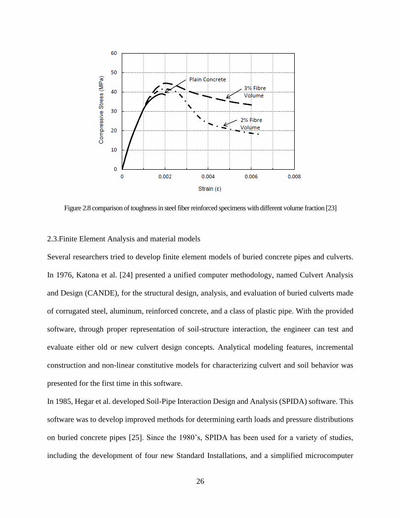
26
Figure 2.8 comparison of toughness in steel fiber reinforced specimens with different volume fraction [23]
2.3.Finite Element Analysis and material models
Several researchers tried to develop finite element models of buried concrete pipes and culverts.
In 1976, Katona et al. [24] presented a unified computer methodology, named Culvert Analysis
and Design (CANDE), for the structural design, analysis, and evaluation of buried culverts made
of corrugated steel, aluminum, reinforced concrete, and a class of plastic pipe. With the provided
software, through proper representation of soil-structure interaction, the engineer can test and
evaluate either old or new culvert design concepts. Analytical modeling features, incremental
construction and non-linear constitutive models for characterizing culvert and soil behavior was
presented for the first time in this software.
In 1985, Hegar et al. developed Soil-Pipe Interaction Design and Analysis (SPIDA) software. This
software was to develop improved methods for determining earth loads and pressure distributions
on buried concrete pipes [25]. Since the 1980’s, SPIDA has been used for a variety of studies,
including the development of four new Standard Installations, and a simplified microcomputer
27
design program, SIDD, Standard Installations Direct Design [2]. These studies were the basis of a
simple indirect design process, proposed by American Concrete Pipe Association (ACPA), for the
design of reinforced concrete pipes.
Kang et al. [26] developed finite element models to investigate the soil-pipe interaction effect in a
trench installation. They identified variables that significantly affect earth loads, as well as the
effects of bedding and side-fill treatments on RCPs and presented the optimum geometry for
imperfect trench installations.
Abolmaali and Kararam [27] developed complete nonlinear three-dimensional finite-element
models of pipe and soil to determine the effect of dynamic compaction forces on RCPs of different
sizes. They verified the results against full-scale experimental testing and predicted the crack
initiation and propagation. They also identified the effects of dynamic forces on the RCPs.
Zhang et al. [28], under various loading conditions, developed a kinematic hardening material
model for the soil to be used for soil-pipe interaction. Using calcareous sand soil, they conducted
experimental tests in the centrifuge resulted in development of a thirteen parameter soil model with
a hardening property.
Tian and Cassidy [29] modified the model developed by Zhang et al. They proposed three models
based on theory of elasticity, which can be used in numerical analysis of pipe–soil interactions. In
their research one dimensional frame elements was used to mimic the structural members in the
FE model. The pipe laying on the ocean bedding was used to observe the behavior of the newly
proposed model However Further studies should be conducted to show the efficiency of the
developed model on buried steel pipes in a trench condition, where different kind of loads are
acting on a buried pipe.
28
Srivastava et al. [30] conducted several laboratory tests PVC pipe buried in trench condition to
investigate the response of the soil–pipe system in terms of load settlement. A two-dimensional
FE model was used to mimic the tests .The tests were performed on small-diameter PVC pipes
(110 mm.
Zarghamee and Tigue [31] developed a 2D FE analysis program named FLEXPIPE. Using this
FE program, to model the soil-pipe interaction, they concluded that there is significant flexural
stresses developed in steel pipes at the invert of the pipe after installation.
Suleiman et al. [32] investigated the effects of large-deflection behavior on buried plastic pipes. In
this study, the results of FE models considering the effect of l large deflections was compared to
the results of the same analysis without the capability to capture large deformation nonlinear
effects. The researchers used ANSYS for their advanced model and CANDE for the simple one.
They reported 10% difference in deflections for the pipes experiencing above 4% deflection with
respect to their diameter.
McGrath [33] conducted a study on pipe–soil interaction during the construction process. Different
backfill materials were used at different compaction levels. Several soil box tests and field tests on
steel, concrete, and plastic pipes were performed to consider the effects of different backfill
materials, trench conditions, trench widths, and bedding materials. The FEM was created
considering a point load on pipe in CANDE and “squeeze method” was applied to mimic the
horizontal effect of compaction on the pipe. The squeeze method does not take into account the
distributive effects of the compaction force on the pipe. As explained by McGrath, modeling the
soil-pipe interaction in flexible pipes without considering the effect of compaction during the
construction is not adequate so the FEM model, which does not consider the effect of compaction,
is incomplete.
29
Dezfooli [34] studied the performance of large-diameter steel pipes embedded and backfilled with
compacted soil material, and installed in trench situation. This research developed A
comprehensive, robust, nonlinear finite element analysis model and the models was verified by
four experimental tests, which were conducted at the University of Texas at Arlington by Najafi
[35] in 2012. The developed FEM model considered all three nonlinear algorithms, including
geometric, material, and contact. The developed FEM model was able to considered the effect of
soil compaction which is an important force in staged construction modeling of the steel pipes.
2.3.1.Constitutive model for Concrete
Post-cracking behavior of fiber reinforced concrete can be introduced in FE analysis with different
numerical softening approaches for crack propagation among which smeared crack, cohesive crack
[36] or fictitious crack models [37] are well known. Models, which are based on cohesive crack,
need the crack path to be predefined before the analysis starts. In these models, a softening curve
for the tensile behavior of the concrete is defined to mimic the crack-unloading process. Interaction
of two surfaces of the cracks will affect the shape of this softening curve therefore; the curve would
be highly dependent to the interaction of the fibers and concrete, which creates the bridging effect.
Cohesive crack models will lead to results that are more precise if the analysis is focused on
development of single cracks in a media. One example of these models is development of the crack
in the basement of concrete embankment dams. For reinforced concrete applications, where there
are several cracks opening during the loading process, using cohesive crack models would not be
applicable. Smeared crack modeling provides a better tool for the RC applications. In this
approach, first introduced by Rashid [38], the cracks are considered to be smeared over the media.
Instead of considering cracks separately, in smeared crack method the material assumed to be
degraded because of the presence of distributed cracks so this method will apply softening
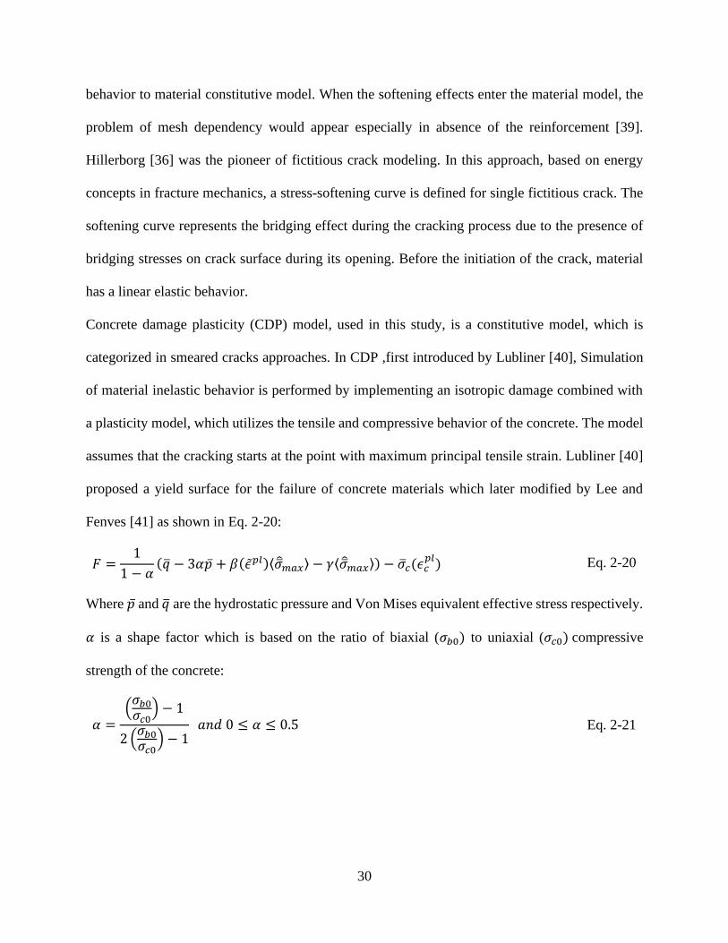
30
behavior to material constitutive model. When the softening effects enter the material model, the
problem of mesh dependency would appear especially in absence of the reinforcement [39].
Hillerborg [36] was the pioneer of fictitious crack modeling. In this approach, based on energy
concepts in fracture mechanics, a stress-softening curve is defined for single fictitious crack. The
softening curve represents the bridging effect during the cracking process due to the presence of
bridging stresses on crack surface during its opening. Before the initiation of the crack, material
has a linear elastic behavior.
Concrete damage plasticity (CDP) model, used in this study, is a constitutive model, which is
categorized in smeared cracks approaches. In CDP ,first introduced by Lubliner [40], Simulation
of material inelastic behavior is performed by implementing an isotropic damage combined with
a plasticity model, which utilizes the tensile and compressive behavior of the concrete. The model
assumes that the cracking starts at the point with maximum principal tensile strain. Lubliner [40]
proposed a yield surface for the failure of concrete materials which later modified by Lee and
Fenves [41] as shown in Eq. 2-20:
𝐹 =1
1 − 𝛼(�̅� − 3𝛼�̅� + 𝛽(𝜖̃𝑝𝑙)⟨�̂̅�𝑚𝑎𝑥⟩ − 𝛾⟨�̂�𝑚𝑎𝑥⟩) − 𝜎𝑐(𝜖𝑐
𝑝𝑙) Eq. 2-20
Where �̅� and �̅� are the hydrostatic pressure and Von Mises equivalent effective stress respectively.
𝛼 is a shape factor which is based on the ratio of biaxial (𝜎𝑏0) to uniaxial (𝜎𝑐0) compressive
strength of the concrete:
𝛼 =(𝜎𝑏0𝜎𝑐0) − 1
2 (𝜎𝑏0𝜎𝑐0) − 1
𝑎𝑛𝑑 0 ≤ 𝛼 ≤ 0.5 Eq. 2-21
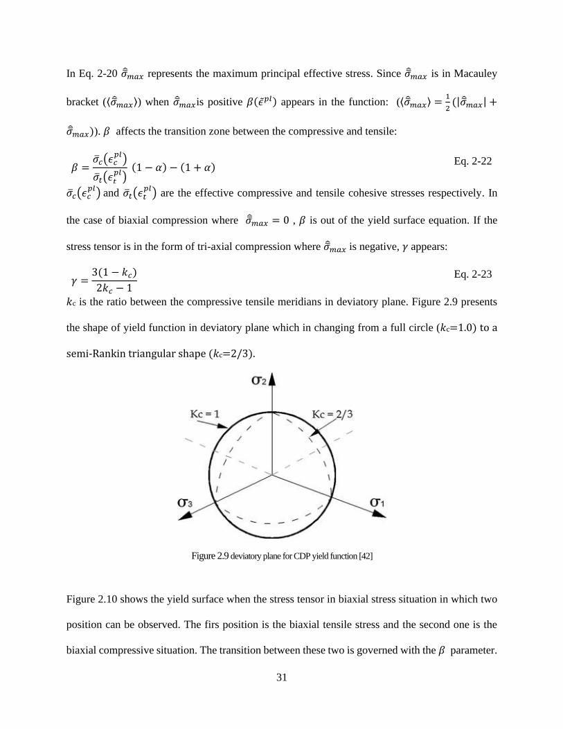
31
In Eq. 2-20 �̂�𝑚𝑎𝑥 represents the maximum principal effective stress. Since �̂�𝑚𝑎𝑥 is in Macauley
bracket (⟨�̂̅�𝑚𝑎𝑥⟩) when �̂�𝑚𝑎𝑥is positive 𝛽(𝜖̃𝑝𝑙) appears in the function: (⟨�̂�𝑚𝑎𝑥⟩ =1
2(|�̂̅�𝑚𝑎𝑥| +
�̂�𝑚𝑎𝑥)). 𝛽 affects the transition zone between the compressive and tensile:
𝛽 =𝜎𝑐(𝜖𝑐
𝑝𝑙)
𝜎𝑡(𝜖𝑡𝑝𝑙) (1 − 𝛼) − (1 + 𝛼)
Eq. 2-22
𝜎𝑐(𝜖𝑐𝑝𝑙) and 𝜎𝑡(𝜖𝑡
𝑝𝑙) are the effective compressive and tensile cohesive stresses respectively. In
the case of biaxial compression where �̂�𝑚𝑎𝑥 = 0 , 𝛽 is out of the yield surface equation. If the
stress tensor is in the form of tri-axial compression where �̂�𝑚𝑎𝑥 is negative, 𝛾 appears:
𝛾 =3(1 − 𝑘𝑐)
2𝑘𝑐 − 1
Eq. 2-23
𝑘c is the ratio between the compressive tensile meridians in deviatory plane. Figure 2.9 presents
the shape of yield function in deviatory plane which in changing from a full circle (𝑘c=1.0) to a
semi-Rankin triangular shape (𝑘c=2/3).
Figure 2.9 deviatory plane for CDP yield function [42]
Figure 2.10 shows the yield surface when the stress tensor in biaxial stress situation in which two
position can be observed. The firs position is the biaxial tensile stress and the second one is the
biaxial compressive situation. The transition between these two is governed with the 𝛽 parameter.
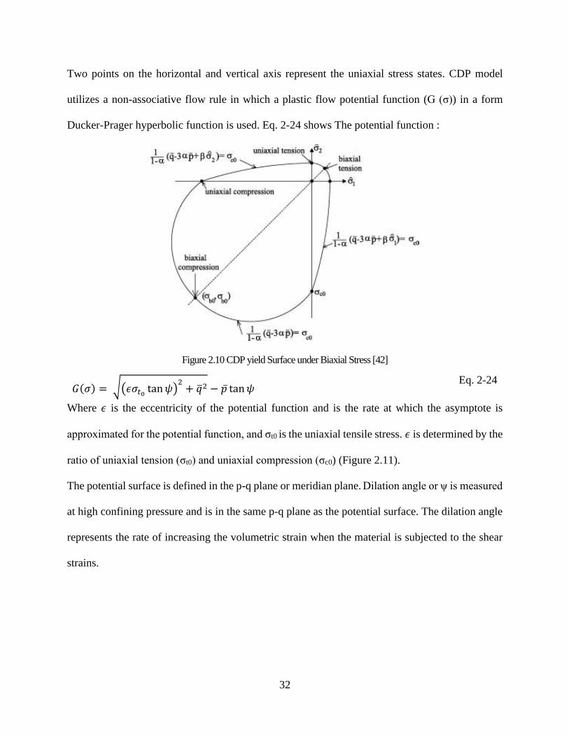
32
Two points on the horizontal and vertical axis represent the uniaxial stress states. CDP model
utilizes a non-associative flow rule in which a plastic flow potential function (G (σ)) in a form
Ducker-Prager hyperbolic function is used. Eq. 2-24 shows The potential function :
Figure 2.10 CDP yield Surface under Biaxial Stress [42]
𝐺(𝜎) = √(𝜖𝜎𝑡0 tan𝜓)2+ �̅�2 − �̅� tan𝜓
Eq. 2-24
Where 𝜖 is the eccentricity of the potential function and is the rate at which the asymptote is
approximated for the potential function, and σt0 is the uniaxial tensile stress. 𝜖 is determined by the
ratio of uniaxial tension (σt0) and uniaxial compression (σc0) (Figure 2.11).
The potential surface is defined in the p-q plane or meridian plane. Dilation angle or ψ is measured
at high confining pressure and is in the same p-q plane as the potential surface. The dilation angle
represents the rate of increasing the volumetric strain when the material is subjected to the shear
strains.
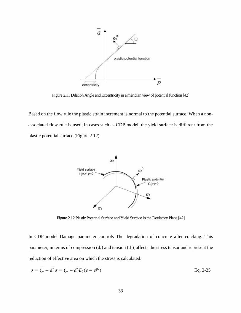
33
Figure 2.11 Dilation Angle and Eccentricity in a meridian view of potential function [42]
Based on the flow rule the plastic strain increment is normal to the potential surface. When a non-
associated flow rule is used, in cases such as CDP model, the yield surface is different from the
plastic potential surface (Figure 2.12).
Figure 2.12 Plastic Potential Surface and Yield Surface in the Deviatory Plane [42]
In CDP model Damage parameter controls The degradation of concrete after cracking. This
parameter, in terms of compression (dc) and tension (dc), affects the stress tensor and represent the
reduction of effective area on which the stress is calculated:
𝜎 = (1 − 𝑑)𝜎 = (1 − 𝑑)𝐸0(𝜖 − 𝜖𝑝𝑙) Eq. 2-25

34
(1 − 𝑑) = (1 − 𝑠𝑡𝑑𝑐)(1 − 𝑠𝑐𝑑𝑡) Eq. 2-26
Where 𝑠𝑡 and 𝑠𝑐 are the stiffness recovery in tension and compression. Figure 2.13 presents the
uniaxial compressive and tensile behavior of the concrete utilized by CDP model to develop the
hardening and softening effects. To prevent the numerical problems due to convergence a viscosity
parameter is introduced to the formulation of CDP. Parameter μ represents the viscosity, which is
based on Duvaut–Lions approach. The viscoelastic strain rate can be obtained by the Eq. 2-27:
𝜖𝑣𝑝𝑙 =
1
𝜇(𝜖𝑝𝑙 − 𝜖𝑣
𝑝𝑙) Eq. 2-27
Figure 2.13 a) uniaxial tensile and b) compressive curves and damage parameter [42]
When the softening effect appears in a material model, the FE mesh size would be one of the
factors on which the model is sensitive. It has been a challenging issue to determine the proper

35
mesh size in concrete material models. To avoid the mesh sensitivity issue, Hillerborg suggested
a fracture energy approach [36]. The approach is based on fracture energy release rate in the brittle
material; it has been shown that if the material property curve is defined by stress-displacement
instead of the stress-strain the mesh sensitivity is highly decreased.
2.3.2.Constitutive model for soil
The soil constitutive models for soil material are available for different purposes in the literature.
They vary from simple to more sophisticated with respect to the information and parameters
needed for creating the model. Thus picking a proper soil constitutive model depends on the
application and the numerical aspects of the model. The most well known available constitutive
models for soil are Hooke’s law (linear elastic model), the Mohr-Coulomb, the Drucker-Prager,
the Duncan-Chang (Hyperbolic model), Cam-Clay (Modified Cam-Clay), Plaxis Soft Soil, and
Plaxis Hardening Soil models [43].
The Mohr-Coulomb model, used in this study, utilizes an elastic-plastic approach with a hardening
effect. This model has been widely used for geotechnical applications. The Mohr-Coulomb model
assumes that the failure of the material is controlled by the maximum shear stress, which depends
on normal stress. This can be represented by plotting the Mohr’s circle for the state of stress tensor
in terms of maximum and minimum principal stresses. The Mohr-Coulomb criterion would be a
line that touches all the failure Mohr’s circles. Figure 2.14 shows the process of creating the line
over the circles. The graphical view leads to Eq. 2-28:
𝜏 = 𝑐 − 𝜎𝑡𝑎𝑛𝜙 Eq. 2-28
Where 𝜏 is the shear stress, 𝜎 is the normal stress (negative in compression), c is the cohesion of
the material, and 𝜙 is the material angle of friction [44]. From the Mohr’s circles geometrical
relationships, 𝜏 and 𝜎 can be represented as follow:
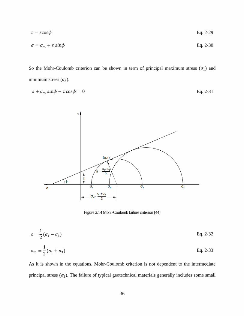
36
𝜏 = 𝑠cos𝜙 Eq. 2-29
𝜎 = 𝜎𝑚 + 𝑠 𝑠𝑖𝑛𝜙 Eq. 2-30
So the Mohr-Coulomb criterion can be shown in term of principal maximum stress (𝜎1) and
minimum stress (𝜎3):
𝑠 + 𝜎𝑚 𝑠𝑖𝑛𝜙 − c cos𝜙 = 0 Eq. 2-31
Figure 2.14 Mohr-Coulomb failure criterion [44]
𝑠 =1
2(𝜎1 − 𝜎3) Eq. 2-32
𝜎𝑚 =1
2(𝜎1 + 𝜎3) Eq. 2-33
As it is shown in the equations, Mohr-Coulomb criterion is not dependent to the intermediate
principal stress (𝜎2). The failure of typical geotechnical materials generally includes some small
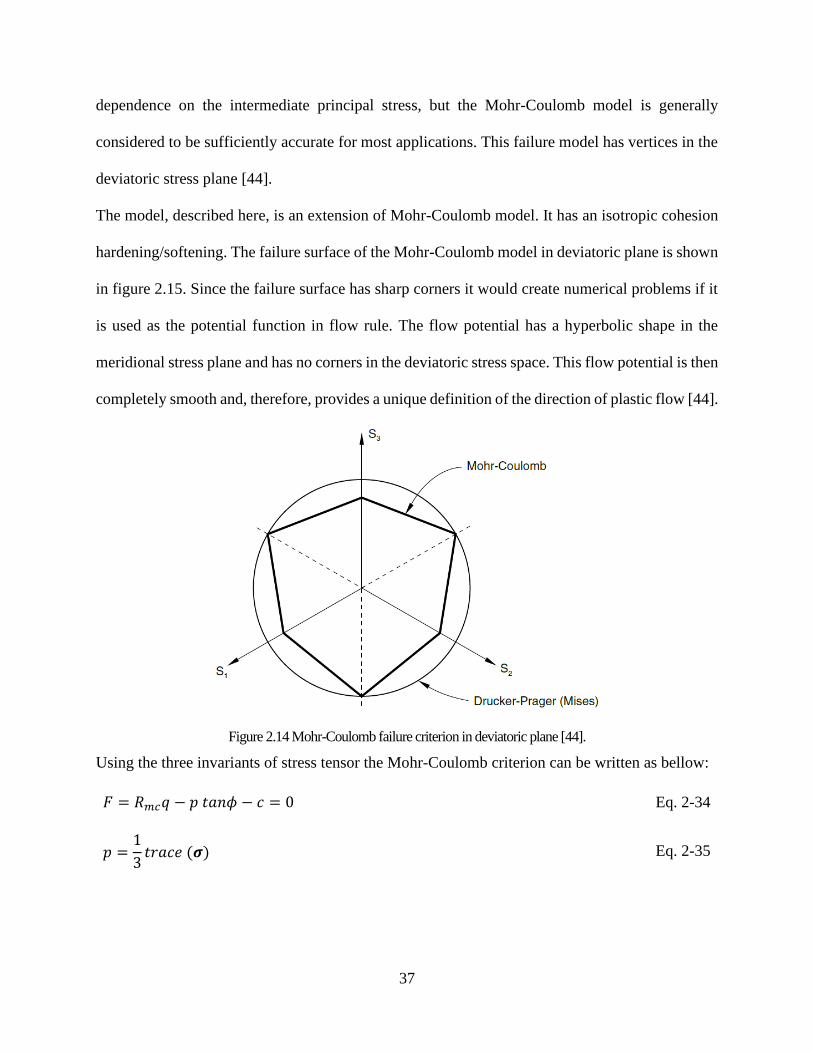
37
dependence on the intermediate principal stress, but the Mohr-Coulomb model is generally
considered to be sufficiently accurate for most applications. This failure model has vertices in the
deviatoric stress plane [44].
The model, described here, is an extension of Mohr-Coulomb model. It has an isotropic cohesion
hardening/softening. The failure surface of the Mohr-Coulomb model in deviatoric plane is shown
in figure 2.15. Since the failure surface has sharp corners it would create numerical problems if it
is used as the potential function in flow rule. The flow potential has a hyperbolic shape in the
meridional stress plane and has no corners in the deviatoric stress space. This flow potential is then
completely smooth and, therefore, provides a unique definition of the direction of plastic flow [44].
Figure 2.14 Mohr-Coulomb failure criterion in deviatoric plane [44].
Using the three invariants of stress tensor the Mohr-Coulomb criterion can be written as bellow:
𝐹 = 𝑅𝑚𝑐𝑞 − 𝑝 𝑡𝑎𝑛𝜙 − 𝑐 = 0 Eq. 2-34
𝑝 =1
3𝑡𝑟𝑎𝑐𝑒 (𝝈) Eq. 2-35
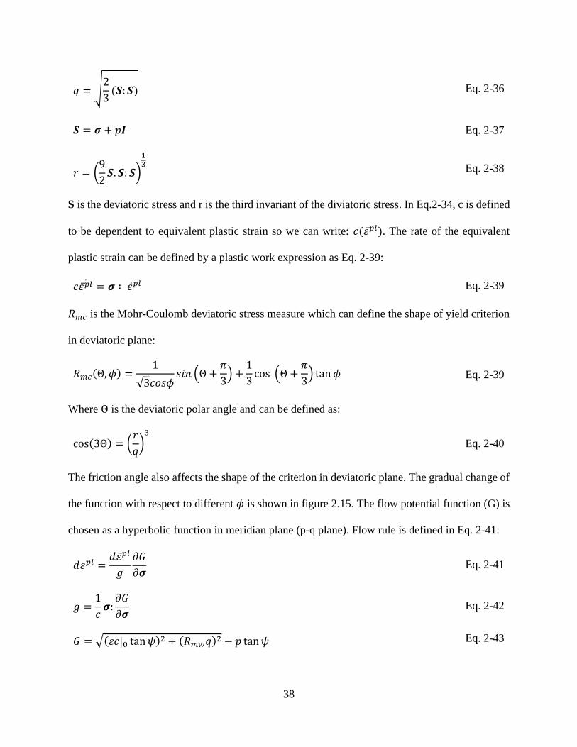
38
𝑞 = √2
3(𝑺: 𝑺) Eq. 2-36
𝑺 = 𝝈 + 𝑝𝑰 Eq. 2-37
𝑟 = (9
2𝑺. 𝑺: 𝑺)
13 Eq. 2-38
S is the deviatoric stress and r is the third invariant of the diviatoric stress. In Eq.2-34, c is defined
to be dependent to equivalent plastic strain so we can write: 𝑐(𝜀̅𝑝𝑙). The rate of the equivalent
plastic strain can be defined by a plastic work expression as Eq. 2-39:
𝑐𝜀�̅�𝑙̇ = 𝝈 ∶ 𝜀̇𝑝𝑙 Eq. 2-39
𝑅𝑚𝑐 is the Mohr-Coulomb deviatoric stress measure which can define the shape of yield criterion
in deviatoric plane:
𝑅𝑚𝑐(Θ, 𝜙) =1
√3𝑐𝑜𝑠𝜙𝑠𝑖𝑛 (Θ +
𝜋
3) +
1
3cos (Θ +
𝜋
3) tan𝜙 Eq. 2-39
Where Θ is the deviatoric polar angle and can be defined as:
cos(3Θ) = (𝑟
𝑞)3
Eq. 2-40
The friction angle also affects the shape of the criterion in deviatoric plane. The gradual change of
the function with respect to different 𝜙 is shown in figure 2.15. The flow potential function (G) is
chosen as a hyperbolic function in meridian plane (p-q plane). Flow rule is defined in Eq. 2-41:
𝑑𝜀𝑝𝑙 =𝑑𝜀̅𝑝𝑙
𝑔
𝜕𝐺
𝜕𝝈 Eq. 2-41
𝑔 =1
𝑐𝝈:𝜕𝐺
𝜕𝝈 Eq. 2-42
𝐺 = √(𝜀𝑐|0 tan𝜓)2 + (𝑅𝑚𝑤𝑞)2 − 𝑝 tan𝜓 Eq. 2-43
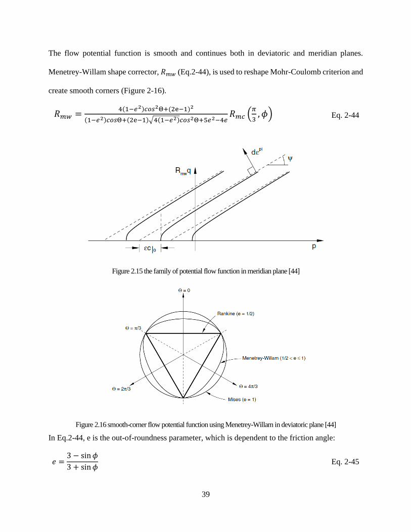
39
The flow potential function is smooth and continues both in deviatoric and meridian planes.
Menetrey-Willam shape corrector, 𝑅𝑚𝑤 (Eq.2-44), is used to reshape Mohr-Coulomb criterion and
create smooth corners (Figure 2-16).
𝑅𝑚𝑤 =4(1−𝑒2)𝑐𝑜𝑠2Θ+(2e−1)2
(1−𝑒2)𝑐𝑜𝑠Θ+(2e−1)√4(1−𝑒2)𝑐𝑜𝑠2Θ+5𝑒2−4𝑒𝑅𝑚𝑐 (
𝜋
3, 𝜙) Eq. 2-44
Figure 2.15 the family of potential flow function in meridian plane [44]
Figure 2.16 smooth-corner flow potential function using Menetrey-Willam in deviatoric plane [44]
In Eq.2-44, e is the out-of-roundness parameter, which is dependent to the friction angle:
𝑒 =3 − sin𝜙
3 + sin𝜙 Eq. 2-45
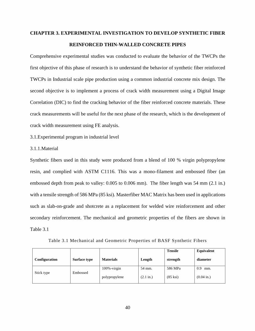
40
CHAPTER 3. EXPERIMENTAL INVESTIGATION TO DEVELOP SYNTHETIC FIBER
REINFORCED THIN-WALLED CONCRETE PIPES
Comprehensive experimental studies was conducted to evaluate the behavior of the TWCPs the
first objective of this phase of research is to understand the behavior of synthetic fiber reinforced
TWCPs in Industrial scale pipe production using a common industrial concrete mix design. The
second objective is to implement a process of crack width measurement using a Digital Image
Correlation (DIC) to find the cracking behavior of the fiber reinforced concrete materials. These
crack measurements will be useful for the next phase of the research, which is the development of
crack width measurement using FE analysis.
3.1.Experimental program in industrial level
3.1.1.Material
Synthetic fibers used in this study were produced from a blend of 100 % virgin polypropylene
resin, and complied with ASTM C1116. This was a mono-filament and embossed fiber (an
embossed depth from peak to valley: 0.005 to 0.006 mm). The fiber length was 54 mm (2.1 in.)
with a tensile strength of 586 MPa (85 ksi). Masterfiber MAC Matrix has been used in applications
such as slab-on-grade and shotcrete as a replacement for welded wire reinforcement and other
secondary reinforcement. The mechanical and geometric properties of the fibers are shown in
Table 3.1
Table 3.1 Mechanical and Geometric Properties of BASF Synthetic Fibers
Configuration Surface type Materials Length
Tensile
strength
Equivalent
diameter
Stick type Embossed
100%-virgin
polypropylene
54 mm.
(2.1 in.)
586 MPa
(85 ksi)
0.9 mm.
(0.04 in.)
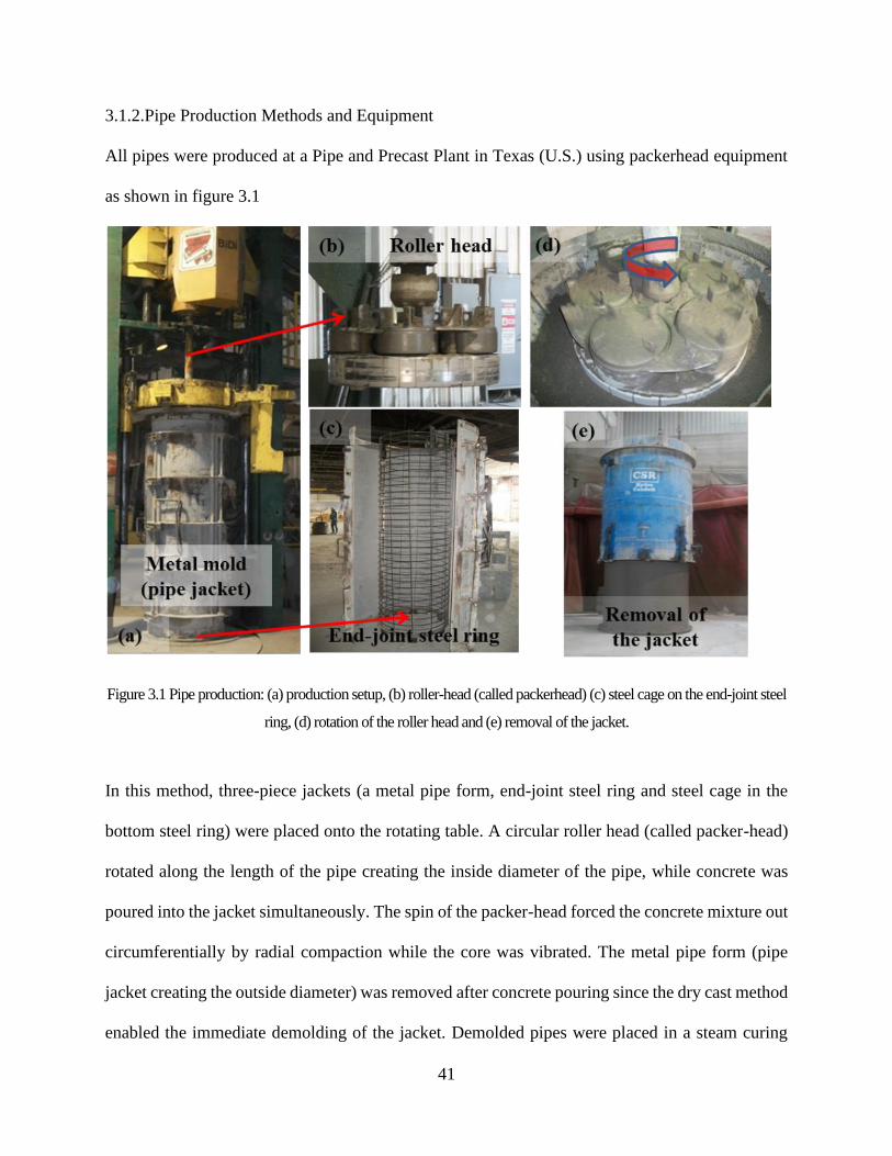
41
3.1.2.Pipe Production Methods and Equipment
All pipes were produced at a Pipe and Precast Plant in Texas (U.S.) using packerhead equipment
as shown in figure 3.1
Figure 3.1 Pipe production: (a) production setup, (b) roller-head (called packerhead) (c) steel cage on the end-joint steel
ring, (d) rotation of the roller head and (e) removal of the jacket.
In this method, three-piece jackets (a metal pipe form, end-joint steel ring and steel cage in the
bottom steel ring) were placed onto the rotating table. A circular roller head (called packer-head)
rotated along the length of the pipe creating the inside diameter of the pipe, while concrete was
poured into the jacket simultaneously. The spin of the packer-head forced the concrete mixture out
circumferentially by radial compaction while the core was vibrated. The metal pipe form (pipe
jacket creating the outside diameter) was removed after concrete pouring since the dry cast method
enabled the immediate demolding of the jacket. Demolded pipes were placed in a steam curing
42
chamber with a temperature of 60ºC (140ºF) for 12 hours and subjected to three-edge bearing tests
after 28 days of production. A low-pressure steam with high humidity and high temperature is
introduced into a chamber, which allows circulation of steam around the entire pipe. Table 3.1
describes the details of pipe specimens created for the experiments.
It should be noted that all pipes in table 3.1 have at least 25 mm (1.0 in. ) concrete cover except
760 mm (36 in.) pipe-series. Forty four test series with the inside diameter ranged from 760 (30
in.) to 3050 mm (120 in.) (pipe length: 2450 mm = 8ft) were created with a combination of the
reduced steel reinforcement (cage reinforcement) and synthetic fibers (Polypropylene fibers). The
three variables are: (1) pipe diameter, (2) the steel reinforcement areas per linear length; and (3)
fiber dosage. Based on the test variables, the nomenclature of test specimens is as follow. The first
number represents the inside diameter of pipes. The second and third characters, “2-0.09” or “8-
0.18”, are the applied fiber dosage and amount of the steel reinforcement. For example, 30-8-0.18
represents that 760 mm (30 in.) inside diameter pipe with 4.8 kg/m3 (8 lb/yd3) and the steel
reinforcement of 3.8 cm2/linear m (0.18 in2/linear ft.) of pipe wall. Based on the evaluation criteria
of concrete pipes with BASF synthetic fiber and reduced traditional steel cage, a test protocol has
been identified. Testing includes 760 mm (30 in.), 910 mm (36 in.), 1370 mm (54 in.), 1520 mm
(60 in.), 1830 mm (72 in.), 2130 mm (84 in.) and 3050 mm (120 in.) diameter pipes, and each test
was repeated two times. First, the reduced circular circumferential steel was designed for flexure
only and synthetic fiber concrete was used to produce the “hybrid” pipes with the above mentioned
large diameter pipes. Next, for each pipe diameter the conventional pipes were produced as
“control” test specimens. Conventional pipes with equal dimension and circular circumferential
steel cages of double layers were tested for comparison.
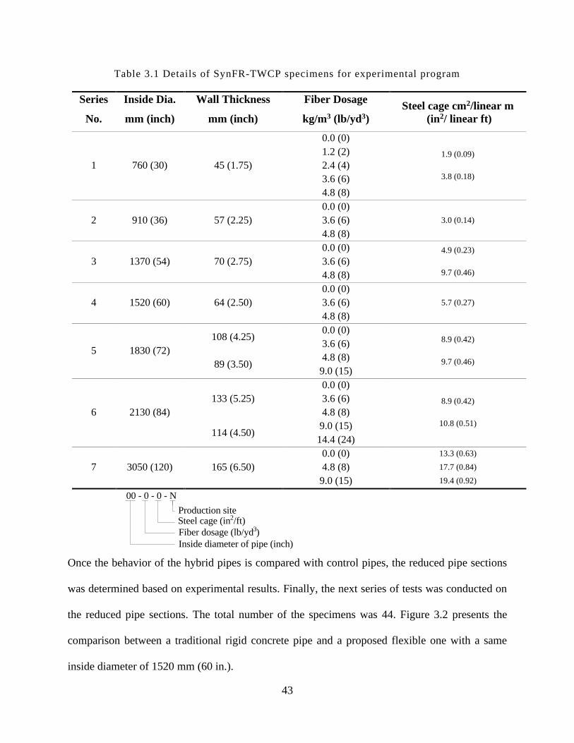
43
Table 3.1 Details of SynFR-TWCP specimens for experimental program
Series
No.
Inside Dia.
mm (inch)
Wall Thickness
mm (inch)
Fiber Dosage
kg/m3 (lb/yd3)
Steel cage cm2/linear m
(in2/ linear ft)
1 760 (30) 45 (1.75)
0.0 (0)
1.9 (0.09)
3.8 (0.18)
1.2 (2)
2.4 (4)
3.6 (6)
4.8 (8)
2 910 (36) 57 (2.25)
0.0 (0)
3.0 (0.14) 3.6 (6)
4.8 (8)
3 1370 (54) 70 (2.75)
0.0 (0) 4.9 (0.23)
9.7 (0.46)
3.6 (6)
4.8 (8)
4 1520 (60) 64 (2.50)
0.0 (0)
5.7 (0.27) 3.6 (6)
4.8 (8)
5 1830 (72)
108 (4.25) 0.0 (0)
8.9 (0.42)
9.7 (0.46)
3.6 (6)
89 (3.50) 4.8 (8)
9.0 (15)
6 2130 (84)
133 (5.25)
0.0 (0)
8.9 (0.42)
10.8 (0.51)
3.6 (6)
4.8 (8)
114 (4.50) 9.0 (15)
14.4 (24)
7 3050 (120) 165 (6.50)
0.0 (0) 13.3 (0.63)
4.8 (8) 17.7 (0.84)
9.0 (15) 19.4 (0.92)
Once the behavior of the hybrid pipes is compared with control pipes, the reduced pipe sections
was determined based on experimental results. Finally, the next series of tests was conducted on
the reduced pipe sections. The total number of the specimens was 44. Figure 3.2 presents the
comparison between a traditional rigid concrete pipe and a proposed flexible one with a same
inside diameter of 1520 mm (60 in.).
00 - 0 - 0 - N
Fiber dosage (lb/yd3)
Steel cage (in2/ft)Production site
Inside diameter of pipe (inch)

44
Figure 3.2 Comparison between RCP and TW pipe (ID: 1520mm=60in.)
3.1.3.TEB tests and observations
As shown in Fig. 3.3 (b), in conventional reinforced concrete pipe the initial crack (first visible
cracks) will be developed when the circumferential tensile stress due to bending in pipe exceeds
the concrete modulus of rupture. This will activate the tensile effect of reinforcement to carry the
load on the tension face of the pipe wall. The D-load corresponding to service load cracks is
designated as D0.3 (D0.01: U.S. unit) with a crack width of 0.3 mm (0.01 in.). The steel strength and
its development length within the pipe wall give the pipe the capability to carry additional load
until it reaches ultimate (Dult), at which failure will happen due to the crushing of the concrete in
compressive part of the wall thickness. When FRCP is loaded to ultimate capacity, however, it has
a larger drop in its load capacity than a conventional RCP of similar ultimate load capacity.
Moreover, as fiber dosages are increased, FRCP may experience a regain in strength after the
observation of the initial cracks (a double peak response with second peak at the post-cracking
stage). Load class is not a directly applicable term for flexible pipes. Installation load carrying
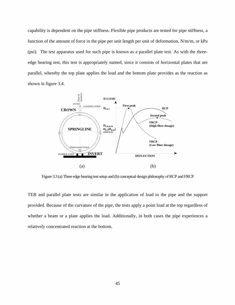
45
capability is dependent on the pipe stiffness. Flexible pipe products are tested for pipe stiffness, a
function of the amount of force in the pipe per unit length per unit of deformation, N/m/m, or kPa
(psi). The test apparatus used for such pipe is known as a parallel plate test. As with the three-
edge bearing test, this test is appropriately named, since it consists of horizontal plates that are
parallel, whereby the top plate applies the load and the bottom plate provides as the reaction as
shown in figure 3.4.
(a) (b)
Figure 3.3 (a) Three edge bearing test setup and (b) conceptual design philosophy of RCP and FRCP
TEB and parallel plate tests are similar in the application of load to the pipe and the support
provided. Because of the curvature of the pipe, the tests apply a point load at the top regardless of
whether a beam or a plate applies the load. Additionally, in both cases the pipe experiences a
relatively concentrated reaction at the bottom.
LOADING STRIP
INVERT
SPRINGLINE
Displacement Sonsor
Pla
nt
of
Sym
met
ry
CROWN
LOAD
RUBBER STRIP
DULT
D0.3(D0.01)(SERVICE)
D-LOAD
DEFLECTION
RCP
FRCP
(High fiber-dosage)
FRCP
(Low fiber-dosage)
First peak
Second peak
DCRACK
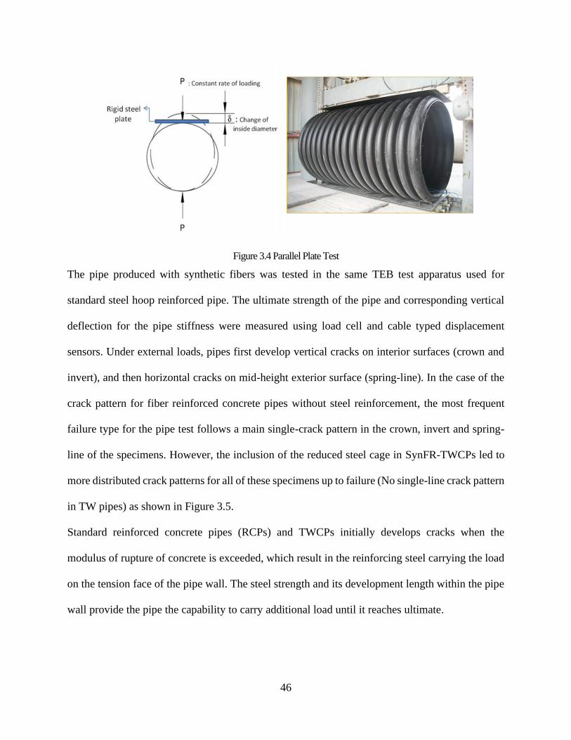
46
Figure 3.4 Parallel Plate Test
The pipe produced with synthetic fibers was tested in the same TEB test apparatus used for
standard steel hoop reinforced pipe. The ultimate strength of the pipe and corresponding vertical
deflection for the pipe stiffness were measured using load cell and cable typed displacement
sensors. Under external loads, pipes first develop vertical cracks on interior surfaces (crown and
invert), and then horizontal cracks on mid-height exterior surface (spring-line). In the case of the
crack pattern for fiber reinforced concrete pipes without steel reinforcement, the most frequent
failure type for the pipe test follows a main single-crack pattern in the crown, invert and spring-
line of the specimens. However, the inclusion of the reduced steel cage in SynFR-TWCPs led to
more distributed crack patterns for all of these specimens up to failure (No single-line crack pattern
in TW pipes) as shown in Figure 3.5.
Standard reinforced concrete pipes (RCPs) and TWCPs initially develops cracks when the
modulus of rupture of concrete is exceeded, which result in the reinforcing steel carrying the load
on the tension face of the pipe wall. The steel strength and its development length within the pipe
wall provide the pipe the capability to carry additional load until it reaches ultimate.
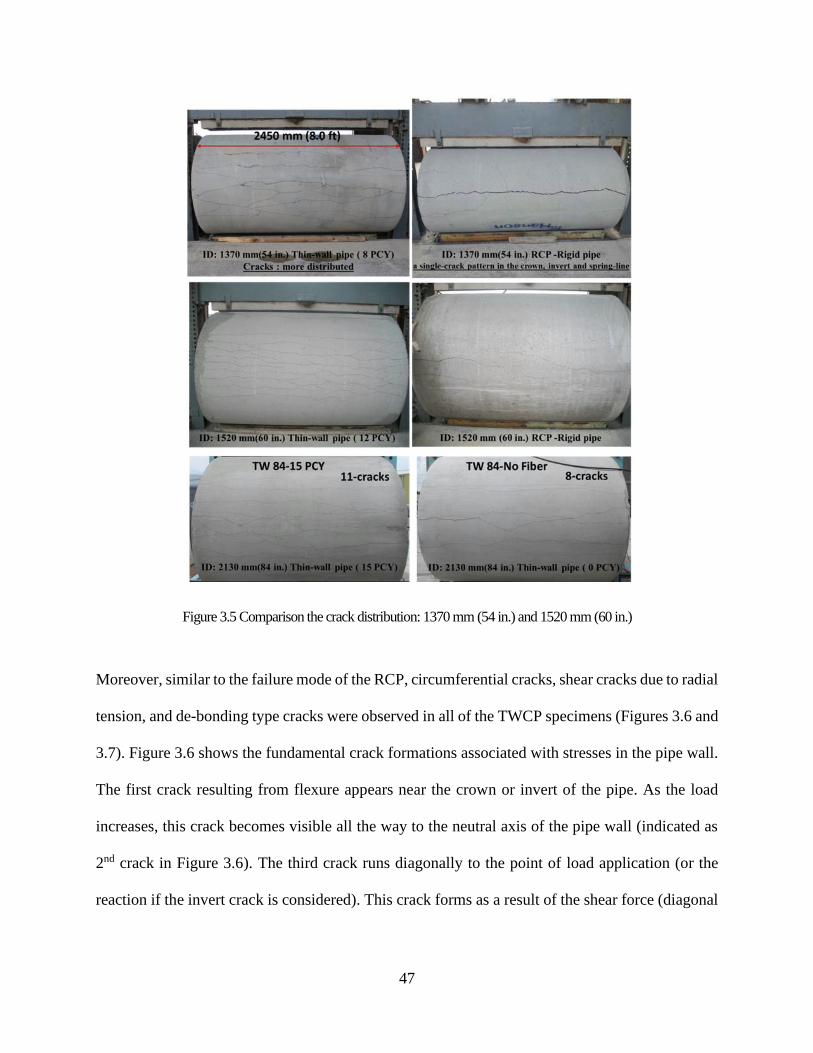
47
Figure 3.5 Comparison the crack distribution: 1370 mm (54 in.) and 1520 mm (60 in.)
Moreover, similar to the failure mode of the RCP, circumferential cracks, shear cracks due to radial
tension, and de-bonding type cracks were observed in all of the TWCP specimens (Figures 3.6 and
3.7). Figure 3.6 shows the fundamental crack formations associated with stresses in the pipe wall.
The first crack resulting from flexure appears near the crown or invert of the pipe. As the load
increases, this crack becomes visible all the way to the neutral axis of the pipe wall (indicated as
2nd crack in Figure 3.6). The third crack runs diagonally to the point of load application (or the
reaction if the invert crack is considered). This crack forms as a result of the shear force (diagonal
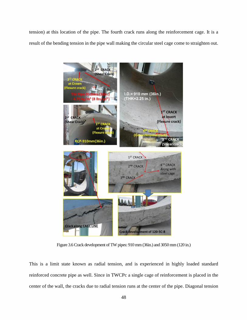
48
tension) at this location of the pipe. The fourth crack runs along the reinforcement cage. It is a
result of the bending tension in the pipe wall making the circular steel cage come to straighten out.
Figure 3.6 Crack development of TW pipes: 910 mm (36in.) and 3050 mm (120 in.)
This is a limit state known as radial tension, and is experienced in highly loaded standard
reinforced concrete pipe as well. Since in TWCPc a single cage of reinforcement is placed in the
center of the wall, the cracks due to radial tension runs at the center of the pipe. Diagonal tension
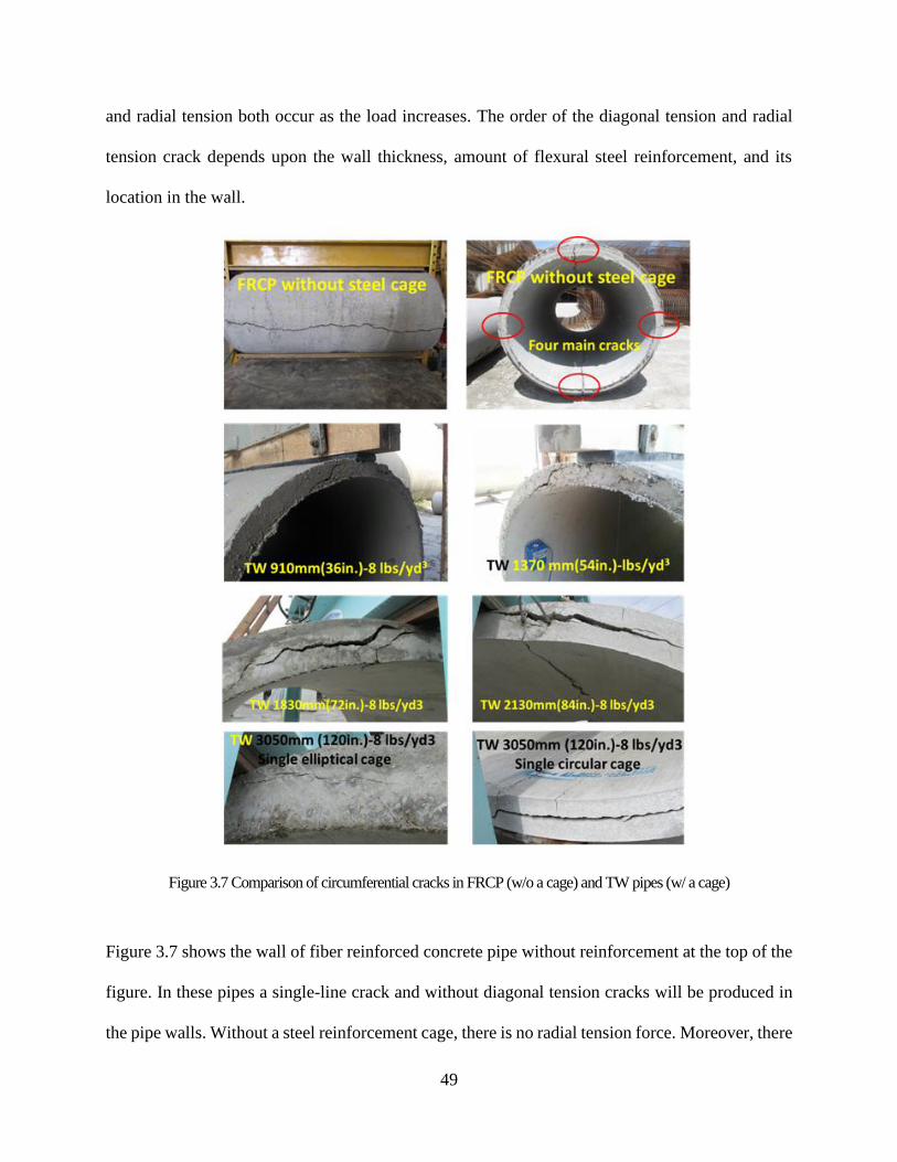
49
and radial tension both occur as the load increases. The order of the diagonal tension and radial
tension crack depends upon the wall thickness, amount of flexural steel reinforcement, and its
location in the wall.
Figure 3.7 Comparison of circumferential cracks in FRCP (w/o a cage) and TW pipes (w/ a cage)
Figure 3.7 shows the wall of fiber reinforced concrete pipe without reinforcement at the top of the
figure. In these pipes a single-line crack and without diagonal tension cracks will be produced in
the pipe walls. Without a steel reinforcement cage, there is no radial tension force. Moreover, there
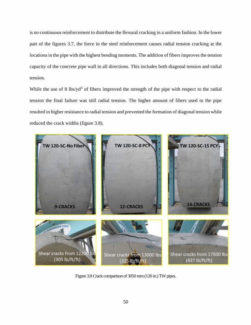
50
is no continuous reinforcement to distribute the flexural cracking in a uniform fashion. In the lower
part of the figures 3.7, the force in the steel reinforcement causes radial tension cracking at the
locations in the pipe with the highest bending moments. The addition of fibers improves the tension
capacity of the concrete pipe wall in all directions. This includes both diagonal tension and radial
tension.
While the use of 8 lbs/yd3 of fibers improved the strength of the pipe with respect to the radial
tension the final failure was still radial tension. The higher amount of fibers used in the pipe
resulted in higher resistance to radial tension and prevented the formation of diagonal tension while
reduced the crack widths (figure 3.8).
Figure 3.8 Crack comparison of 3050 mm (120 in.) TW pipes.
51
3.1.4.Load deformation curves
Load-deflection curves were obtained for the majority of the tested Pipes, which described the
vertical deflection of the pipe due to the load being applied along its length. Except 3050 mm (120
in.) thin walled specimens, all specimens were tested to reach over 5 % deflection of the pipe
diameter. The comparisons of the load-deflection plots for the pipes with synthetic fiber
reinforcement are shown and summarized in figure 3.9 to figure 3.11 and Table 3-2. The change
in geometry and reinforcement of the pipes is described in a combined parameter of Diameter,
thickness and reinforcement area: D
t×As . In load-deflection curves as the reinforcement increases
the initial stiffness of the pipes increases. Consequently, the pipe strength increased with an
increase in the steel reinforcement. For the pipe thickness, same results were observed. The
stiffness of the pipe before the first crack and the pipe strength increased with an increase of the
pipe thickness. The addition of fiber dosage led the increase of the pipe strength. This might be
attributed to the crack holding capacity by bridging shear cracks at the top and bottom of the pipes.
As the fiber dosage increased, the strength of the pipes increased as well. Most TWCPs maintained
bending stiffness up to 3% deflection of inside diameter. A summary of load deflection curves are
presented in figures 3.12 and 3.13.
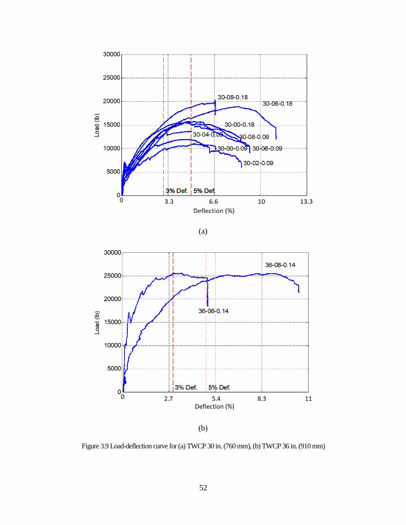
52
(a)
(b)
Figure 3.9 Load-deflection curve for (a) TWCP 30 in. (760 mm), (b) TWCP 36 in. (910 mm)
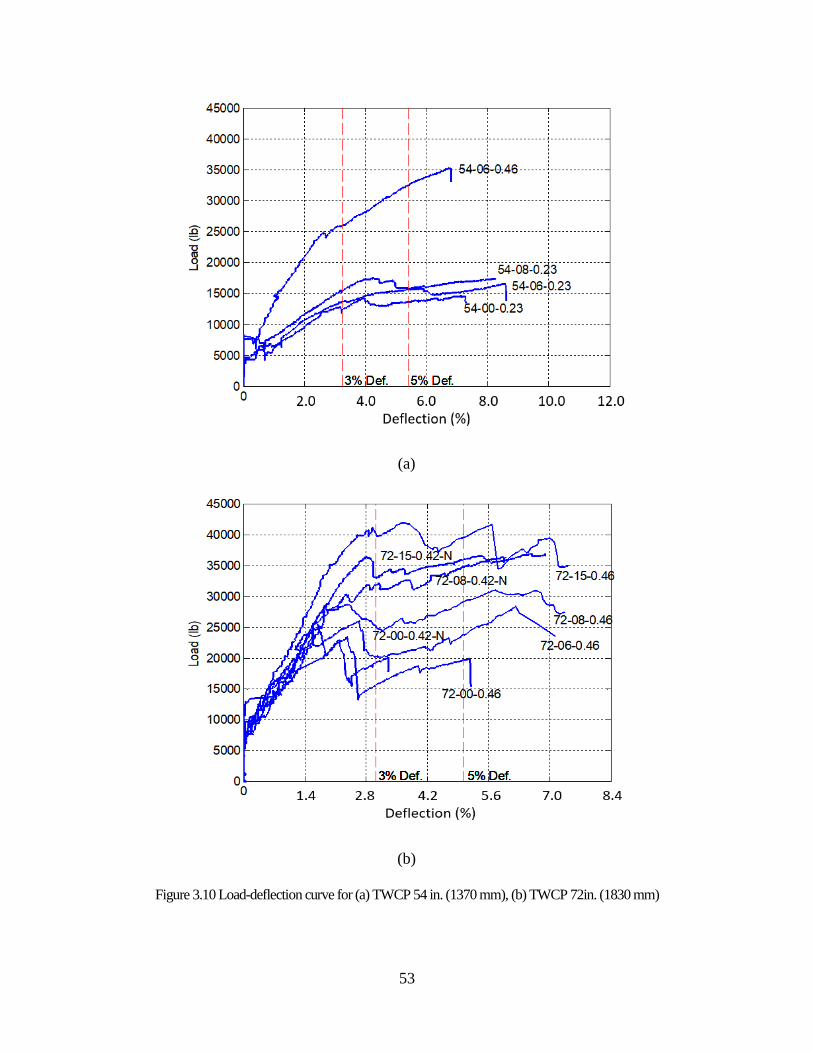
53
(a)
(b)
Figure 3.10 Load-deflection curve for (a) TWCP 54 in. (1370 mm), (b) TWCP 72in. (1830 mm)
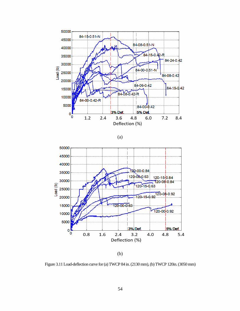
54
(a)
(b)
Figure 3.11 Load-deflection curve for (a) TWCP 84 in. (2130 mm), (b) TWCP 120in. (3050 mm)
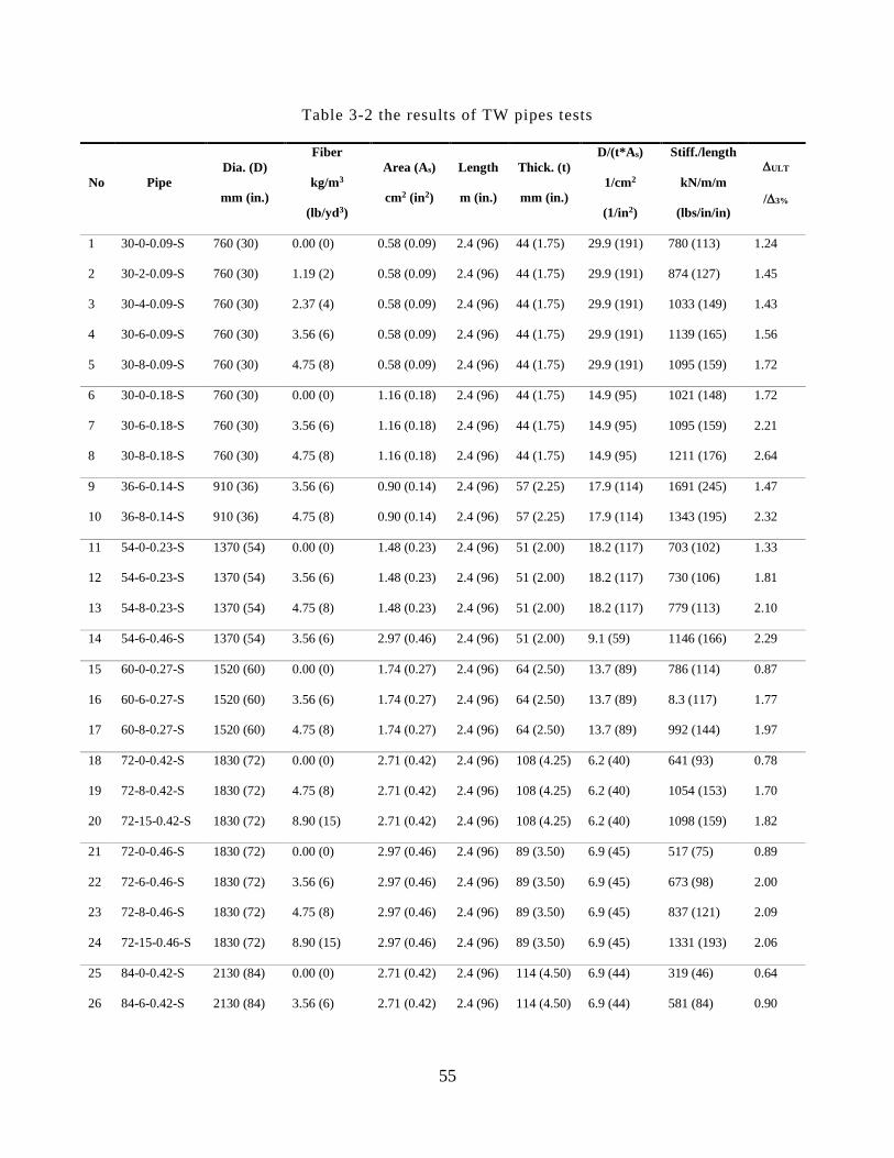
55
Table 3-2 the results of TW pipes tests
No Pipe
Dia. (D)
mm (in.)
Fiber
kg/m3
(lb/yd3)
Area (As)
cm2 (in2)
Length
m (in.)
Thick. (t)
mm (in.)
D/(t*As)
1/cm2
(1/in2)
Stiff./length
kN/m/m
(lbs/in/in)
ULT
/3%
1 30-0-0.09-S 760 (30) 0.00 (0) 0.58 (0.09) 2.4 (96) 44 (1.75) 29.9 (191) 780 (113) 1.24
2 30-2-0.09-S 760 (30) 1.19 (2) 0.58 (0.09) 2.4 (96) 44 (1.75) 29.9 (191) 874 (127) 1.45
3 30-4-0.09-S 760 (30) 2.37 (4) 0.58 (0.09) 2.4 (96) 44 (1.75) 29.9 (191) 1033 (149) 1.43
4 30-6-0.09-S 760 (30) 3.56 (6) 0.58 (0.09) 2.4 (96) 44 (1.75) 29.9 (191) 1139 (165) 1.56
5 30-8-0.09-S 760 (30) 4.75 (8) 0.58 (0.09) 2.4 (96) 44 (1.75) 29.9 (191) 1095 (159) 1.72
6 30-0-0.18-S 760 (30) 0.00 (0) 1.16 (0.18) 2.4 (96) 44 (1.75) 14.9 (95) 1021 (148) 1.72
7 30-6-0.18-S 760 (30) 3.56 (6) 1.16 (0.18) 2.4 (96) 44 (1.75) 14.9 (95) 1095 (159) 2.21
8 30-8-0.18-S 760 (30) 4.75 (8) 1.16 (0.18) 2.4 (96) 44 (1.75) 14.9 (95) 1211 (176) 2.64
9 36-6-0.14-S 910 (36) 3.56 (6) 0.90 (0.14) 2.4 (96) 57 (2.25) 17.9 (114) 1691 (245) 1.47
10 36-8-0.14-S 910 (36) 4.75 (8) 0.90 (0.14) 2.4 (96) 57 (2.25) 17.9 (114) 1343 (195) 2.32
11 54-0-0.23-S 1370 (54) 0.00 (0) 1.48 (0.23) 2.4 (96) 51 (2.00) 18.2 (117) 703 (102) 1.33
12 54-6-0.23-S 1370 (54) 3.56 (6) 1.48 (0.23) 2.4 (96) 51 (2.00) 18.2 (117) 730 (106) 1.81
13 54-8-0.23-S 1370 (54) 4.75 (8) 1.48 (0.23) 2.4 (96) 51 (2.00) 18.2 (117) 779 (113) 2.10
14 54-6-0.46-S 1370 (54) 3.56 (6) 2.97 (0.46) 2.4 (96) 51 (2.00) 9.1 (59) 1146 (166) 2.29
15 60-0-0.27-S 1520 (60) 0.00 (0) 1.74 (0.27) 2.4 (96) 64 (2.50) 13.7 (89) 786 (114) 0.87
16 60-6-0.27-S 1520 (60) 3.56 (6) 1.74 (0.27) 2.4 (96) 64 (2.50) 13.7 (89) 8.3 (117) 1.77
17 60-8-0.27-S 1520 (60) 4.75 (8) 1.74 (0.27) 2.4 (96) 64 (2.50) 13.7 (89) 992 (144) 1.97
18 72-0-0.42-S 1830 (72) 0.00 (0) 2.71 (0.42) 2.4 (96) 108 (4.25) 6.2 (40) 641 (93) 0.78
19 72-8-0.42-S 1830 (72) 4.75 (8) 2.71 (0.42) 2.4 (96) 108 (4.25) 6.2 (40) 1054 (153) 1.70
20 72-15-0.42-S 1830 (72) 8.90 (15) 2.71 (0.42) 2.4 (96) 108 (4.25) 6.2 (40) 1098 (159) 1.82
21 72-0-0.46-S 1830 (72) 0.00 (0) 2.97 (0.46) 2.4 (96) 89 (3.50) 6.9 (45) 517 (75) 0.89
22 72-6-0.46-S 1830 (72) 3.56 (6) 2.97 (0.46) 2.4 (96) 89 (3.50) 6.9 (45) 673 (98) 2.00
23 72-8-0.46-S 1830 (72) 4.75 (8) 2.97 (0.46) 2.4 (96) 89 (3.50) 6.9 (45) 837 (121) 2.09
24 72-15-0.46-S 1830 (72) 8.90 (15) 2.97 (0.46) 2.4 (96) 89 (3.50) 6.9 (45) 1331 (193) 2.06
25 84-0-0.42-S 2130 (84) 0.00 (0) 2.71 (0.42) 2.4 (96) 114 (4.50) 6.9 (44) 319 (46) 0.64
26 84-6-0.42-S 2130 (84) 3.56 (6) 2.71 (0.42) 2.4 (96) 114 (4.50) 6.9 (44) 581 (84) 0.90
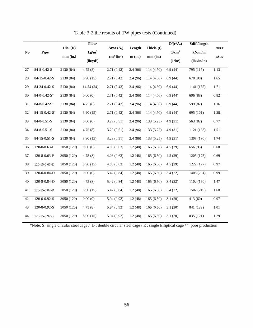
56
Table 3-2 the results of TW pipes tests (Continued)
No Pipe
Dia. (D)
mm (in.)
Fiber
kg/m3
(lb/yd3)
Area (As)
cm2 (in2)
Length
m (in.)
Thick. (t)
mm (in.)
D/(t*As)
1/cm2
(1/in2)
Stiff./length
kN/m/m
(lbs/in/in)
ULT
/3%
27 84-8-0.42-S 2130 (84) 4.75 (8) 2.71 (0.42) 2.4 (96) 114 (4.50) 6.9 (44) 795 (115) 1.13
28 84-15-0.42-S 2130 (84) 8.90 (15) 2.71 (0.42) 2.4 (96) 114 (4.50) 6.9 (44) 678 (98) 1.65
29 84-24-0.42-S 2130 (84) 14.24 (24) 2.71 (0.42) 2.4 (96) 114 (4.50) 6.9 (44) 1141 (165) 1.71
30 84-0-0.42-S+ 2130 (84) 0.00 (0) 2.71 (0.42) 2.4 (96) 114 (4.50) 6.9 (44) 606 (88) 0.82
31 84-8-0.42-S+ 2130 (84) 4.75 (8) 2.71 (0.42) 2.4 (96) 114 (4.50) 6.9 (44) 599 (87) 1.16
32 84-15-0.42-S+ 2130 (84) 8.90 (15) 2.71 (0.42) 2.4 (96) 114 (4.50) 6.9 (44) 695 (101) 1.38
33 84-0-0.51-S 2130 (84) 0.00 (0) 3.29 (0.51) 2.4 (96) 133 (5.25) 4.9 (31) 563 (82) 0.77
34 84-8-0.51-S 2130 (84) 4.75 (8) 3.29 (0.51) 2.4 (96) 133 (5.25) 4.9 (31) 1121 (163) 1.51
35 84-15-0.51-S 2130 (84) 8.90 (15) 3.29 (0.51) 2.4 (96) 133 (5.25) 4.9 (31) 1308 (190) 1.74
36 120-0-0.63-E 3050 (120) 0.00 (0) 4.06 (0.63) 1.2 (48) 165 (6.50) 4.5 (29) 656 (95) 0.60
37 120-8-0.63-E 3050 (120) 4.75 (8) 4.06 (0.63) 1.2 (48) 165 (6.50) 4.5 (29) 1205 (175) 0.69
38 120-15-0.63-E 3050 (120) 8.90 (15) 4.06 (0.63) 1.2 (48) 165 (6.50) 4.5 (29) 1222 (177) 0.97
39 120-0-0.84-D 3050 (120) 0.00 (0) 5.42 (0.84) 1.2 (48) 165 (6.50) 3.4 (22) 1405 (204) 0.99
40 120-8-0.84-D 3050 (120) 4.75 (8) 5.42 (0.84) 1.2 (48) 165 (6.50) 3.4 (22) 1102 (160) 1.47
41 120-15-0.84-D 3050 (120) 8.90 (15) 5.42 (0.84) 1.2 (48) 165 (6.50) 3.4 (22) 1507 (219) 1.60
42 120-0-0.92-S 3050 (120) 0.00 (0) 5.94 (0.92) 1.2 (48) 165 (6.50) 3.1 (20) 413 (60) 0.97
43 120-8-0.92-S 3050 (120) 4.75 (8) 5.94 (0.92) 1.2 (48) 165 (6.50) 3.1 (20) 841 (122) 1.01
44 120-15-0.92-S 3050 (120) 8.90 (15) 5.94 (0.92) 1.2 (48) 165 (6.50) 3.1 (20) 835 (121) 1.29
*Note: S: single circular steel cage / D : double circular steel cage / E : single Elliptical cage / +: poor production
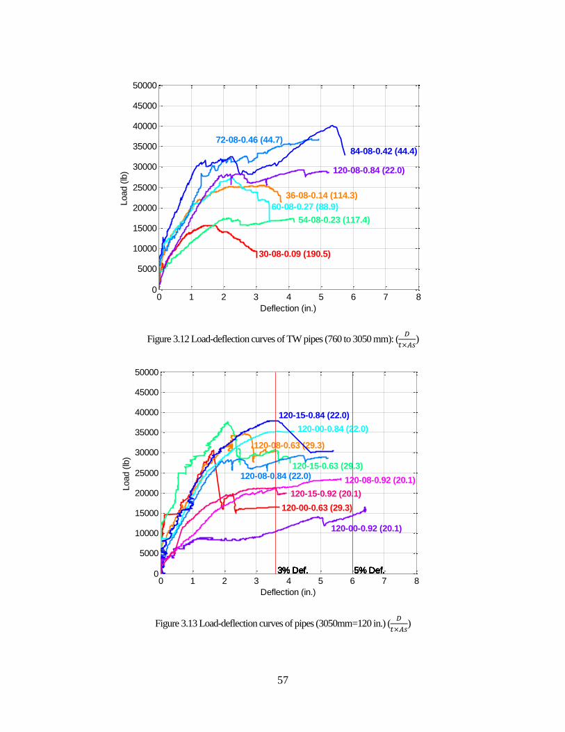
57
Figure 3.12 Load-deflection curves of TW pipes (760 to 3050 mm): (𝐷
𝑡×𝐴𝑠)
Figure 3.13 Load-deflection curves of pipes (3050mm=120 in.) (𝐷
𝑡×𝐴𝑠)
0 1 2 3 4 5 6 7 80
5000
10000
15000
20000
25000
30000
35000
40000
45000
50000
30-08-0.09 (190.5)
Deflection (in.)
Load (
lb)
36-08-0.14 (114.3)
54-08-0.23 (117.4)
60-08-0.27 (88.9)
72-08-0.46 (44.7)
84-08-0.42 (44.4)
120-08-0.84 (22.0)
0 1 2 3 4 5 6 7 80
5000
10000
15000
20000
25000
30000
35000
40000
45000
50000
Deflection (in.)
Load (
lb)
3% Def. 5% Def.
120-00-0.63 (29.3)
3% Def. 5% Def.
120-08-0.63 (29.3)
3% Def. 5% Def.
120-15-0.63 (29.3)
3% Def. 5% Def.
120-00-0.84 (22.0)
3% Def. 5% Def.
120-08-0.84 (22.0)
3% Def. 5% Def.
120-15-0.84 (22.0)
3% Def. 5% Def.
120-00-0.92 (20.1)
3% Def. 5% Def.
120-08-0.92 (20.1)
3% Def. 5% Def.
120-15-0.92 (20.1)
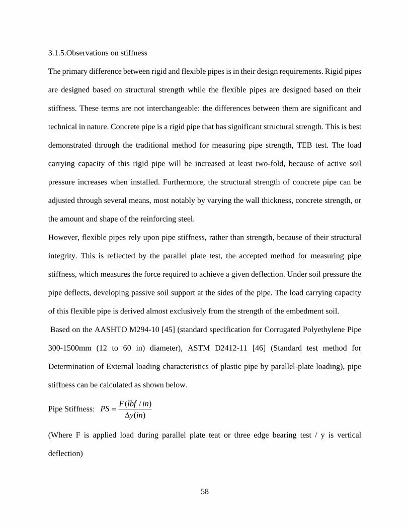
58
3.1.5.Observations on stiffness
The primary difference between rigid and flexible pipes is in their design requirements. Rigid pipes
are designed based on structural strength while the flexible pipes are designed based on their
stiffness. These terms are not interchangeable: the differences between them are significant and
technical in nature. Concrete pipe is a rigid pipe that has significant structural strength. This is best
demonstrated through the traditional method for measuring pipe strength, TEB test. The load
carrying capacity of this rigid pipe will be increased at least two-fold, because of active soil
pressure increases when installed. Furthermore, the structural strength of concrete pipe can be
adjusted through several means, most notably by varying the wall thickness, concrete strength, or
the amount and shape of the reinforcing steel.
However, flexible pipes rely upon pipe stiffness, rather than strength, because of their structural
integrity. This is reflected by the parallel plate test, the accepted method for measuring pipe
stiffness, which measures the force required to achieve a given deflection. Under soil pressure the
pipe deflects, developing passive soil support at the sides of the pipe. The load carrying capacity
of this flexible pipe is derived almost exclusively from the strength of the embedment soil.
Based on the AASHTO M294-10 [45] (standard specification for Corrugated Polyethylene Pipe
300-1500mm (12 to 60 in) diameter), ASTM D2412-11 [46] (Standard test method for
Determination of External loading characteristics of plastic pipe by parallel-plate loading), pipe
stiffness can be calculated as shown below.
Pipe Stiffness: ( / )
( )
F lbf inPS
y in=
(Where F is applied load during parallel plate teat or three edge bearing test / y is vertical
deflection)
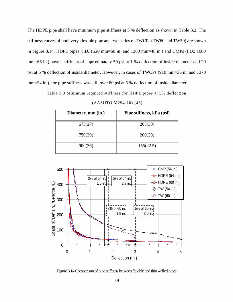
59
The HDPE pipe shall have minimum pipe stiffness at 5 % deflection as shown in Table 3.3. The
stiffness curves of both very-flexible pipe and two series of TWCPs (TW60 and TW50) are shown
in Figure 3.14. HDPE pipes (I.D.:1520 mm=60 in. and 1200 mm=48 in.) and CMPs (I.D.: 1680
mm=66 in.) have a stiffness of approximately 50 psi at 1 % deflection of inside diameter and 20
psi at 5 % deflection of inside diameter. However, in cases of TWCPs (910 mm=36 in. and 1370
mm=54 in.), the pipe stiffness was still over 80 psi at 5 % deflection of inside diameter.
Table 3.3 Minimum required stiffness for HDPE pipes at 5% deflection
(AASHTO M294-10) [46]
Diameter, mm (in.) Pipe stiffness, kPa (psi)
675(27) 205(30)
750(30) 200(29)
900(36) 155(22.5)
Figure 3.14 Comparison of pipe stiffness between flexible and thin walled pipes
0
100
200
300
400
500
0 1 2 3 4 5
Deflection (in.)
Load(l
b)/
Def.
(in.)
/Length
(in.) a
CMP (54 in.)
HDPE (54 in.)
HDPE (60 in.)
TW (54 in.)
TW (60 in.)
3% of 54 in.
= 1.6 in.
5% of 54 in.
= 2.7 in.
3% of 60 in.
= 1.8 in.
5% of 60 in.
= 3.0 in.
60
Among forty-four specimens tested, thirty-eight TW pipes (84 % of test pipes) satisfy minimum
stiffness of 100 psi before adding the synthetic fiber in concrete mixture. However, based on the
consideration of the inclusion of synthetic fibers into TWCPs, only one pipe (86-6-0.42) failed to
satisfy the minimum pipe stiffness of 100 psi among thirty-four TWCPs with synthetic fibers. That
is, 97 % of tested TW pipes with fibers passed the minimum pipe stiffness of 100 psi. Compared
with the minimum pipe stiffness of flexible pipes by AASHTO M294-11 [45] and ASTM F405
[46], TECPs showed superior stiffness than flexible pipes such as HDPE pipes and CMPs.
3.1.6.Conclusions of the TWCP tests
The innovative TW concrete pipe system, known as flexible concrete pipe, has the advantages of
thinner pipe wall and lighter weight. The concept and philosophy to reach the above objectives is
the fact that discrete synthetic fibers increase the shear capacity of concrete, delaying the shear
failure mode, and significantly enhancing the pipe’s load carrying capacity with the use of reduced
steel reinforcement. This allows a reduction in wall thickness for a specified stiffness. The
reductions in pipe thickness in these experiments were in the ranges of 35% and 50% for small
and large diameter concrete pipe, respectively.
The capability of the TW pipe for Deformation toward the surrounding soil is considered as the
key factor to behave as a flexible concrete pipe. To fulfill this capability the TW pipe should have
enough deflection (more than 3%) as well as a minimum stiffness. To have a guideline it is set for
TW pipes to have a minimum stiffness of 690 kPa (100 psi) at 3 % deflection. Among thirty-four
tested TW pipes with synthetic fibers, thirty-two TW pipes (97 %) satisfied the suggested
minimum pipe stiffness (100 psi) at 3% deflection. with the large amount of deformation in TW
pipes the method of crack control is very important in the design process. A reliable design should
be able to control the cracks of the pipes because of large deflections and should have a well

61
stablished definition of the acceptable level of crack width in TW pipes. The results of the TWCP
tests is used in chapter 3 to verify the FE models of TEB tests.
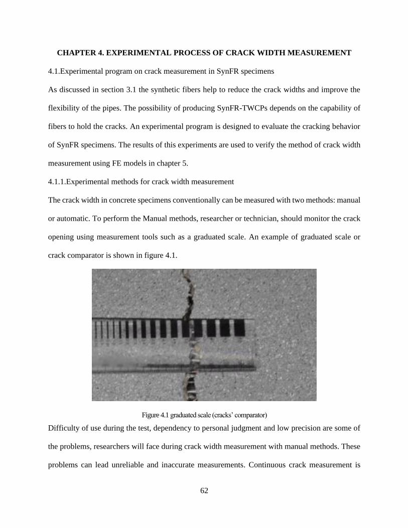
62
CHAPTER 4. EXPERIMENTAL PROCESS OF CRACK WIDTH MEASUREMENT
4.1.Experimental program on crack measurement in SynFR specimens
As discussed in section 3.1 the synthetic fibers help to reduce the crack widths and improve the
flexibility of the pipes. The possibility of producing SynFR-TWCPs depends on the capability of
fibers to hold the cracks. An experimental program is designed to evaluate the cracking behavior
of SynFR specimens. The results of this experiments are used to verify the method of crack width
measurement using FE models in chapter 5.
4.1.1.Experimental methods for crack width measurement
The crack width in concrete specimens conventionally can be measured with two methods: manual
or automatic. To perform the Manual methods, researcher or technician, should monitor the crack
opening using measurement tools such as a graduated scale. An example of graduated scale or
crack comparator is shown in figure 4.1.
Figure 4.1 graduated scale (cracks’ comparator)
Difficulty of use during the test, dependency to personal judgment and low precision are some of
the problems, researchers will face during crack width measurement with manual methods. These
problems can lead unreliable and inaccurate measurements. Continuous crack measurement is
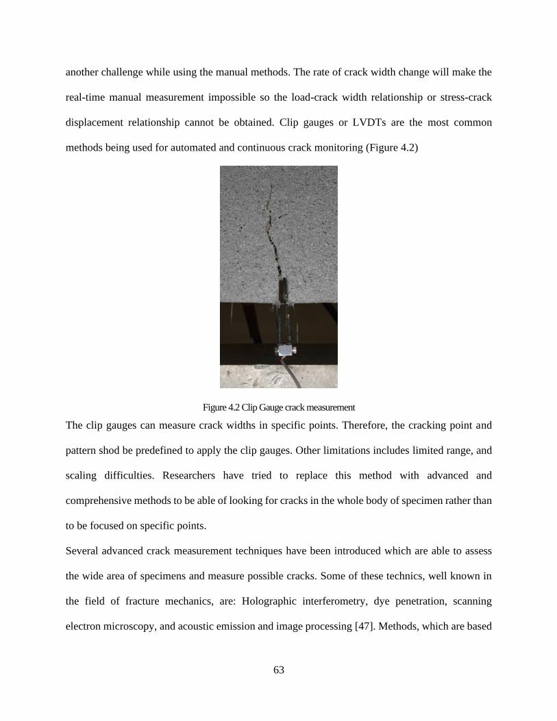
63
another challenge while using the manual methods. The rate of crack width change will make the
real-time manual measurement impossible so the load-crack width relationship or stress-crack
displacement relationship cannot be obtained. Clip gauges or LVDTs are the most common
methods being used for automated and continuous crack monitoring (Figure 4.2)
Figure 4.2 Clip Gauge crack measurement
The clip gauges can measure crack widths in specific points. Therefore, the cracking point and
pattern shod be predefined to apply the clip gauges. Other limitations includes limited range, and
scaling difficulties. Researchers have tried to replace this method with advanced and
comprehensive methods to be able of looking for cracks in the whole body of specimen rather than
to be focused on specific points.
Several advanced crack measurement techniques have been introduced which are able to assess
the wide area of specimens and measure possible cracks. Some of these technics, well known in
the field of fracture mechanics, are: Holographic interferometry, dye penetration, scanning
electron microscopy, and acoustic emission and image processing [47]. Methods, which are based
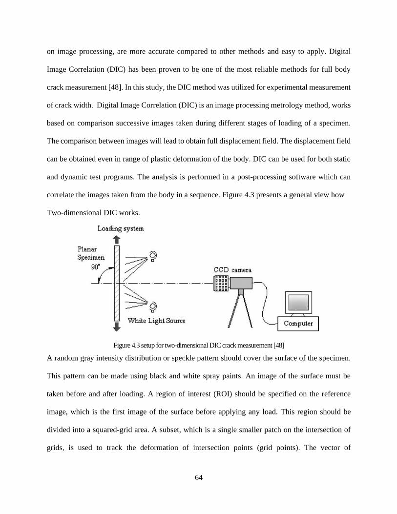
64
on image processing, are more accurate compared to other methods and easy to apply. Digital
Image Correlation (DIC) has been proven to be one of the most reliable methods for full body
crack measurement [48]. In this study, the DIC method was utilized for experimental measurement
of crack width. Digital Image Correlation (DIC) is an image processing metrology method, works
based on comparison successive images taken during different stages of loading of a specimen.
The comparison between images will lead to obtain full displacement field. The displacement field
can be obtained even in range of plastic deformation of the body. DIC can be used for both static
and dynamic test programs. The analysis is performed in a post-processing software which can
correlate the images taken from the body in a sequence. Figure 4.3 presents a general view how
Two-dimensional DIC works.
Figure 4.3 setup for two-dimensional DIC crack measurement [48]
A random gray intensity distribution or speckle pattern should cover the surface of the specimen.
This pattern can be made using black and white spray paints. An image of the surface must be
taken before and after loading. A region of interest (ROI) should be specified on the reference
image, which is the first image of the surface before applying any load. This region should be
divided into a squared-grid area. A subset, which is a single smaller patch on the intersection of
grids, is used to track the deformation of intersection points (grid points). The vector of
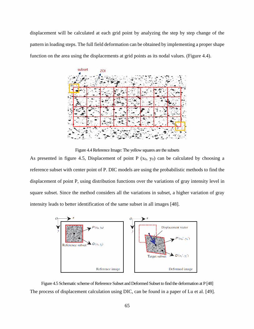
65
displacement will be calculated at each grid point by analyzing the step by step change of the
pattern in loading steps. The full field deformation can be obtained by implementing a proper shape
function on the area using the displacements at grid points as its nodal values. (Figure 4.4).
Figure 4.4 Reference Image: The yellow squares are the subsets
As presented in figure 4.5, Displacement of point P (x0, y0) can be calculated by choosing a
reference subset with center point of P. DIC models are using the probabilistic methods to find the
displacement of point P, using distribution functions over the variations of gray intensity level in
square subset. Since the method considers all the variations in subset, a higher variation of gray
intensity leads to better identification of the same subset in all images [48].
Figure 4.5 Schematic scheme of Reference Subset and Deformed Subset to find the deformation at P [48]
The process of displacement calculation using DIC, can be found in a paper of Lu et al. [49].

66
4.1.2.Details of experimental program
Two series of flexural specimens were casted with a dry-cast mix design, using two volume
fractions of synthetic fibers. Synthetic fibers with volume fractions of 0.54% (8.3 pound per cubic
yard (PCY)) and 1.04% (16 PCY) were used. The total number of flexural specimens were 12, 6
specimens with each volume fraction of fibers.
Using ASTM standard specimens, the uniaxial compression test was performed to obtain the
maximum compressive capacity of the synthetic FRC specimens. Two series of tests were
designed for the Flexural specimens: Three-point bending of notched beams and four-point
bending of unnotched beams.
based on the recommendation of RILEM TC 162TDF [50] for fiber reinforced concrete, a test
setup was designed and loading process was performed on three-point bending specimens.
Recommendations of ASTM C1609/C 1609M – 12 [51] were used to perform the four-point
bending tests. The Loading history and mid-span deflection were recorded during the flexural tests.
The surface deformation and crack propagation of the specimens was obtained using two-
dimensional DIC technique. A set of preliminary verification experiments proved the accuracy of
two-dimensional DIC technique by using three-point bending test with clip gauges. In these
experiments Crack mouth opening displacement (CMOD) of the notched beam specimens,
obtained with a clip gauge transducer during the tests, were compared with the results of two-
dimensional DIC method. After verification process the load-crack width curves were derived for
all the tests specimens using DIC method.
Three-point bending tests were performed on beams 6 inches wide and 6 inches deep, and 20
inches long (6x6x20 in) with notch of 1-inch depth and less than 0.2 inches width. The notch was
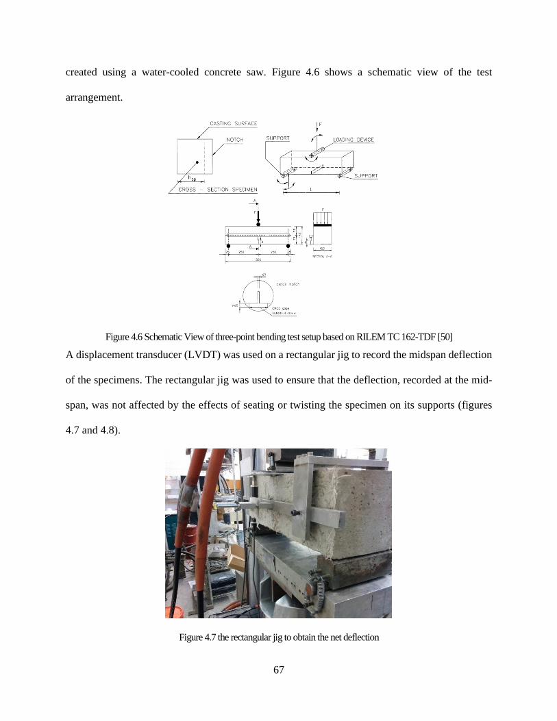
67
created using a water-cooled concrete saw. Figure 4.6 shows a schematic view of the test
arrangement.
Figure 4.6 Schematic View of three-point bending test setup based on RILEM TC 162-TDF [50]
A displacement transducer (LVDT) was used on a rectangular jig to record the midspan deflection
of the specimens. The rectangular jig was used to ensure that the deflection, recorded at the mid-
span, was not affected by the effects of seating or twisting the specimen on its supports (figures
4.7 and 4.8).
Figure 4.7 the rectangular jig to obtain the net deflection
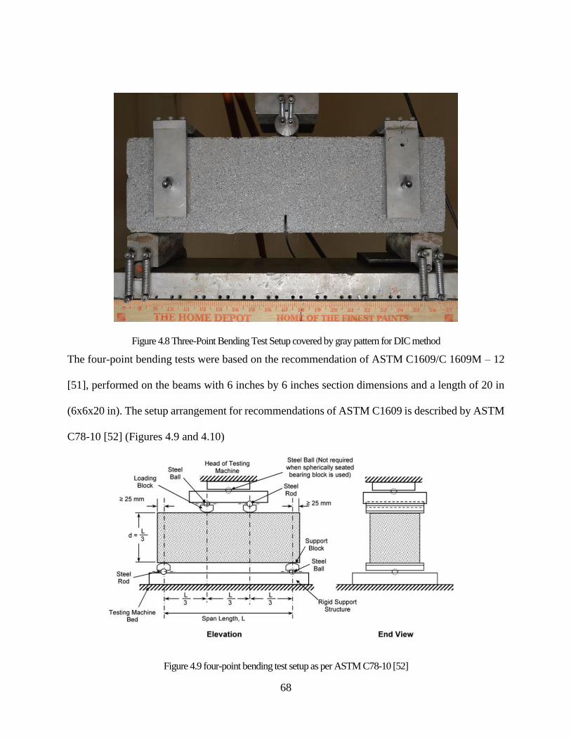
68
Figure 4.8 Three-Point Bending Test Setup covered by gray pattern for DIC method
The four-point bending tests were based on the recommendation of ASTM C1609/C 1609M – 12
[51], performed on the beams with 6 inches by 6 inches section dimensions and a length of 20 in
(6x6x20 in). The setup arrangement for recommendations of ASTM C1609 is described by ASTM
C78-10 [52] (Figures 4.9 and 4.10)
Figure 4.9 four-point bending test setup as per ASTM C78-10 [52]

69
Same as Three-point bending tests, mid-span net deflection of the beams was recorded during the
test, using a displacement transducer (LVDT) mounted to a rectangular jig (Figure 4.10 and
4.11).
Figure 4.10 LVDT and jig arrangement to measure the mid-span deflection four-point bending test
Figure 4.11 Test Setup for 4-Point Bending Test
During both kind of tests a MTS machine was used to insert displacement-control loading. The
loading rate was kept constant for all the beam specimens at a rate of 0.2 mm/min (0.0079 in/min).
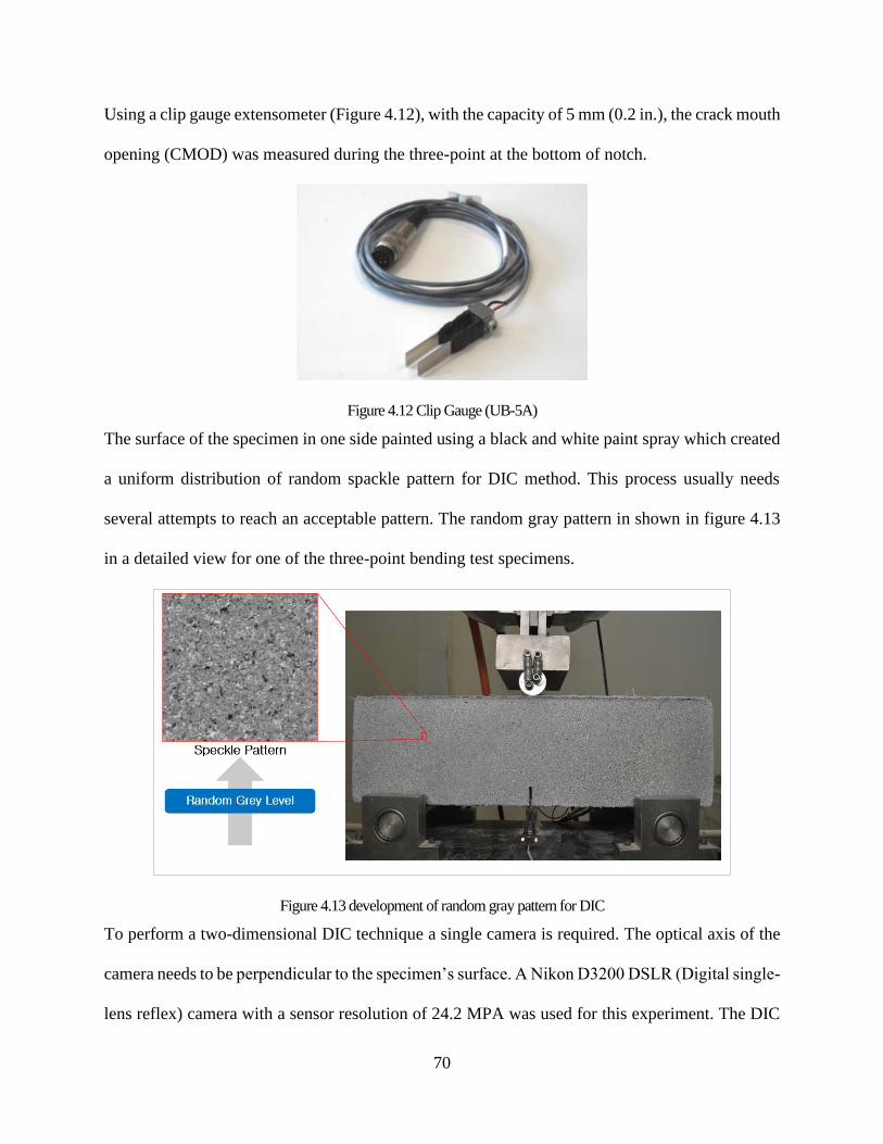
70
Using a clip gauge extensometer (Figure 4.12), with the capacity of 5 mm (0.2 in.), the crack mouth
opening (CMOD) was measured during the three-point at the bottom of notch.
Figure 4.12 Clip Gauge (UB-5A)
The surface of the specimen in one side painted using a black and white paint spray which created
a uniform distribution of random spackle pattern for DIC method. This process usually needs
several attempts to reach an acceptable pattern. The random gray pattern in shown in figure 4.13
in a detailed view for one of the three-point bending test specimens.
Figure 4.13 development of random gray pattern for DIC
To perform a two-dimensional DIC technique a single camera is required. The optical axis of the
camera needs to be perpendicular to the specimen’s surface. A Nikon D3200 DSLR (Digital single-
lens reflex) camera with a sensor resolution of 24.2 MPA was used for this experiment. The DIC
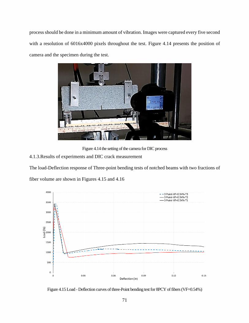
71
process should be done in a minimum amount of vibration. Images were captured every five second
with a resolution of 6016x4000 pixels throughout the test. Figure 4.14 presents the position of
camera and the specimen during the test.
Figure 4.14 the setting of the camera for DIC process
4.1.3.Results of experiments and DIC crack measurement
The load-Deflection response of Three-point bending tests of notched beams with two fractions of
fiber volume are shown in Figures 4.15 and 4.16
Figure 4.15 Load - Deflection curves of three-Point bending test for 8PCY of fibers (VF=0.54%)
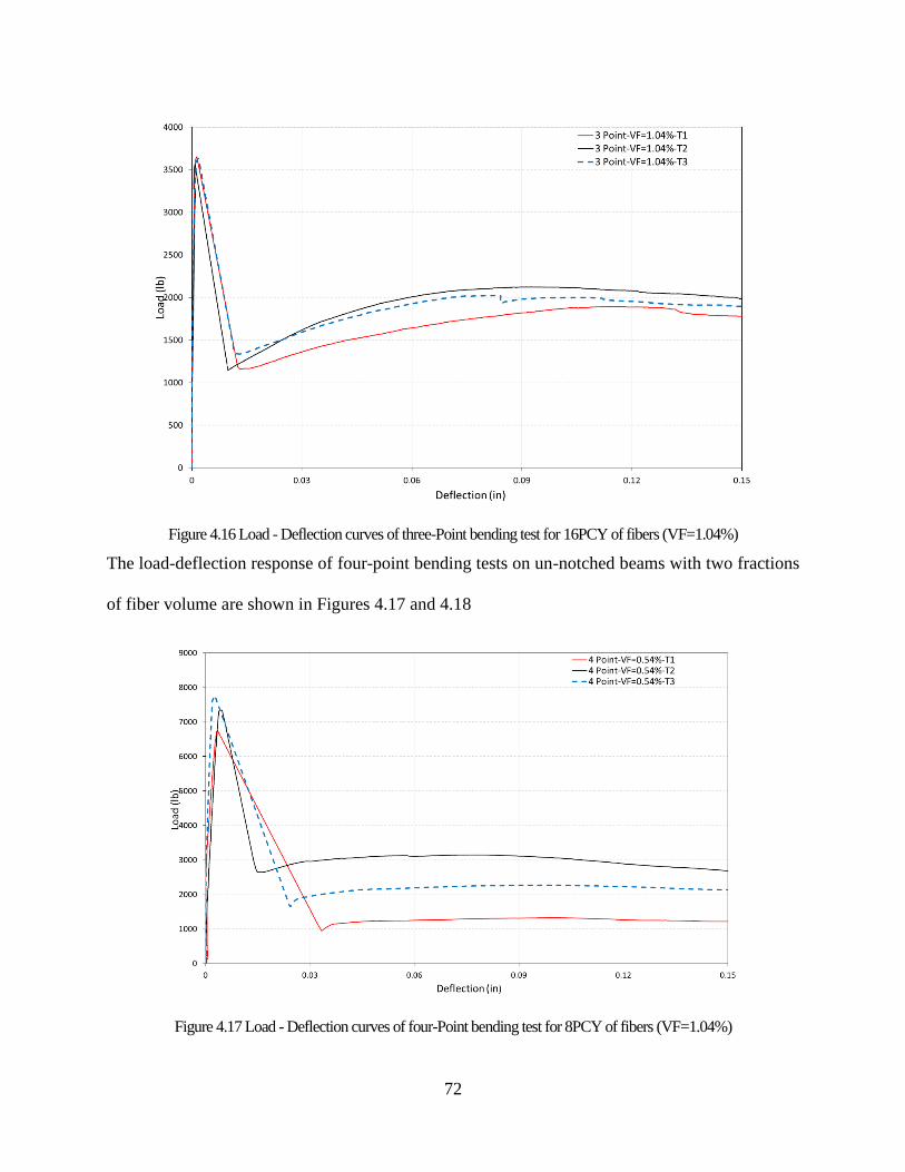
72
Figure 4.16 Load - Deflection curves of three-Point bending test for 16PCY of fibers (VF=1.04%)
The load-deflection response of four-point bending tests on un-notched beams with two fractions
of fiber volume are shown in Figures 4.17 and 4.18
Figure 4.17 Load - Deflection curves of four-Point bending test for 8PCY of fibers (VF=1.04%)
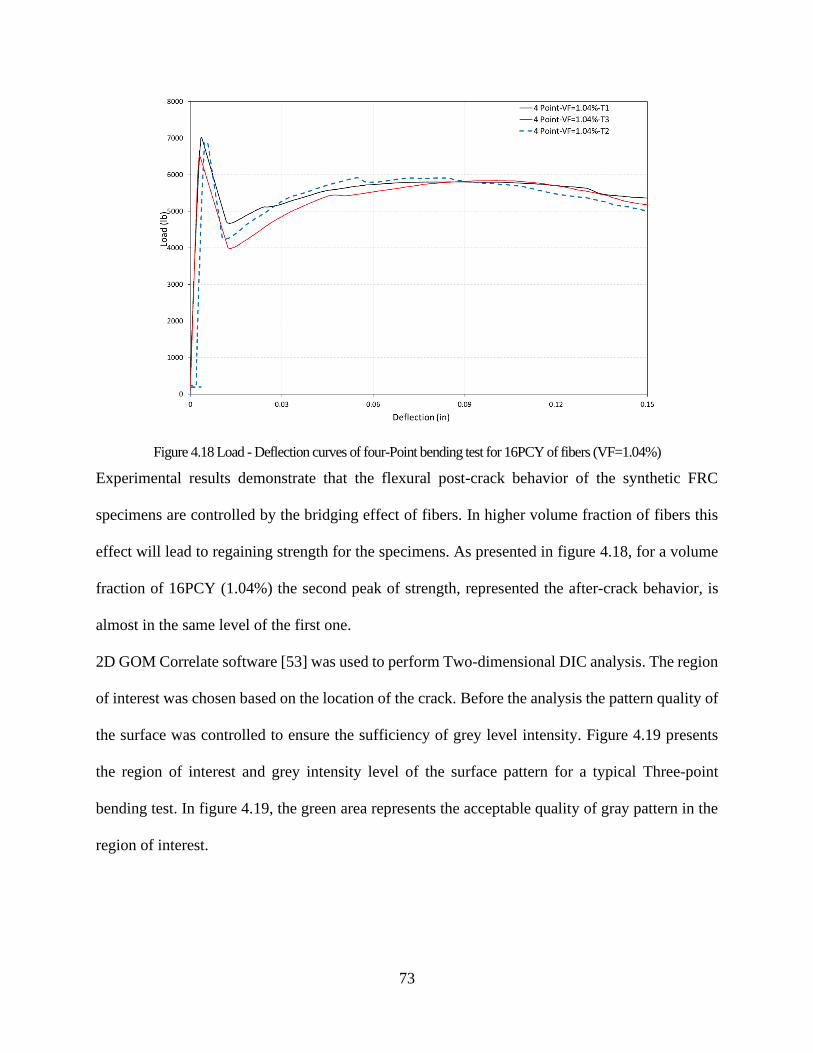
73
Figure 4.18 Load - Deflection curves of four-Point bending test for 16PCY of fibers (VF=1.04%)
Experimental results demonstrate that the flexural post-crack behavior of the synthetic FRC
specimens are controlled by the bridging effect of fibers. In higher volume fraction of fibers this
effect will lead to regaining strength for the specimens. As presented in figure 4.18, for a volume
fraction of 16PCY (1.04%) the second peak of strength, represented the after-crack behavior, is
almost in the same level of the first one.
2D GOM Correlate software [53] was used to perform Two-dimensional DIC analysis. The region
of interest was chosen based on the location of the crack. Before the analysis the pattern quality of
the surface was controlled to ensure the sufficiency of grey level intensity. Figure 4.19 presents
the region of interest and grey intensity level of the surface pattern for a typical Three-point
bending test. In figure 4.19, the green area represents the acceptable quality of gray pattern in the
region of interest.
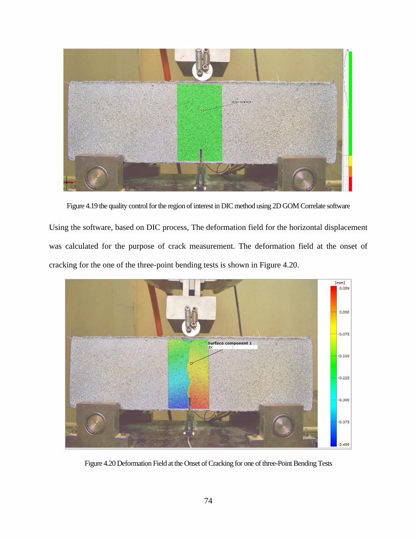
74
Figure 4.19 the quality control for the region of interest in DIC method using 2D GOM Correlate software
Using the software, based on DIC process, The deformation field for the horizontal displacement
was calculated for the purpose of crack measurement. The deformation field at the onset of
cracking for the one of the three-point bending tests is shown in Figure 4.20.
Figure 4.20 Deformation Field at the Onset of Cracking for one of three-Point Bending Tests
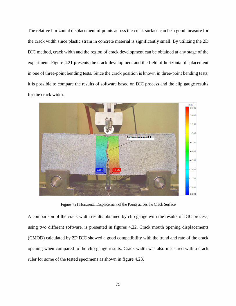
75
The relative horizontal displacement of points across the crack surface can be a good measure for
the crack width since plastic strain in concrete material is significantly small. By utilizing the 2D
DIC method, crack width and the region of crack development can be obtained at any stage of the
experiment. Figure 4.21 presents the crack development and the field of horizontal displacement
in one of three-point bending tests. Since the crack position is known in three-point bending tests,
it is possible to compare the results of software based on DIC process and the clip gauge results
for the crack width.
Figure 4.21 Horizontal Displacement of the Points across the Crack Surface
A comparison of the crack width results obtained by clip gauge with the results of DIC process,
using two different software, is presented in figures 4.22. Crack mouth opening displacements
(CMOD) calculated by 2D DIC showed a good compatibility with the trend and rate of the crack
opening when compared to the clip gauge results. Crack width was also measured with a crack
ruler for some of the tested specimens as shown in figure 4.23.
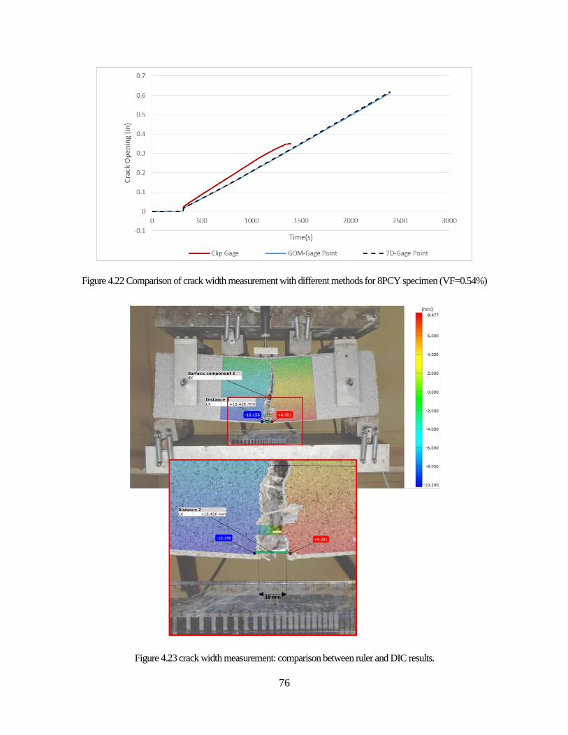
76
Figure 4.22 Comparison of crack width measurement with different methods for 8PCY specimen (VF=0.54%)
Figure 4.23 crack width measurement: comparison between ruler and DIC results.
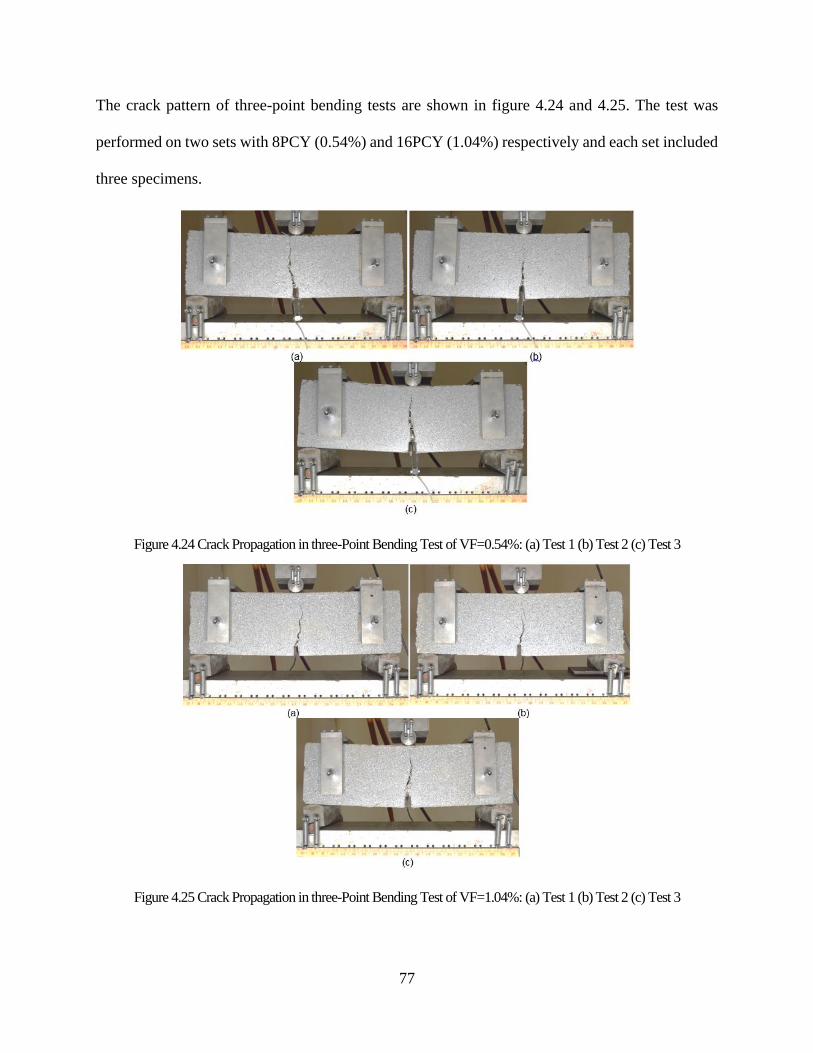
77
The crack pattern of three-point bending tests are shown in figure 4.24 and 4.25. The test was
performed on two sets with 8PCY (0.54%) and 16PCY (1.04%) respectively and each set included
three specimens.
Figure 4.24 Crack Propagation in three-Point Bending Test of VF=0.54%: (a) Test 1 (b) Test 2 (c) Test 3
Figure 4.25 Crack Propagation in three-Point Bending Test of VF=1.04%: (a) Test 1 (b) Test 2 (c) Test 3
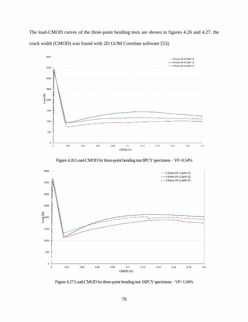
78
The load-CMOD curves of the three-point bending tests are shown in figures 4.26 and 4.27. the
crack width (CMOD) was found with 2D GOM Correlate software [53].
Figure 4.26 Load-CMOD for three-point bending test 8PCY specimens – VF=0.54%
Figure 4.27 Load-CMOD for three-point bending test 16PCY specimens – VF=1.04%

79
The crack pattern of four -point bending tests are shown in figure 4.28 and 4.29. the test was
performed on two sets with 8PCY (0.54%) and 16PCY (1.04%) respectively and each set included
three specimens.
Figure 4.28 Crack Propagation in four-Point Bending Test of VF=0.54%: (a) Test 1 (b) Test 2 (c) Test 3
Figure 4.29 Crack Propagation in four-Point Bending Test of VF=1.04%: (a) Test 1 (b) Test 2 (c) Test 3
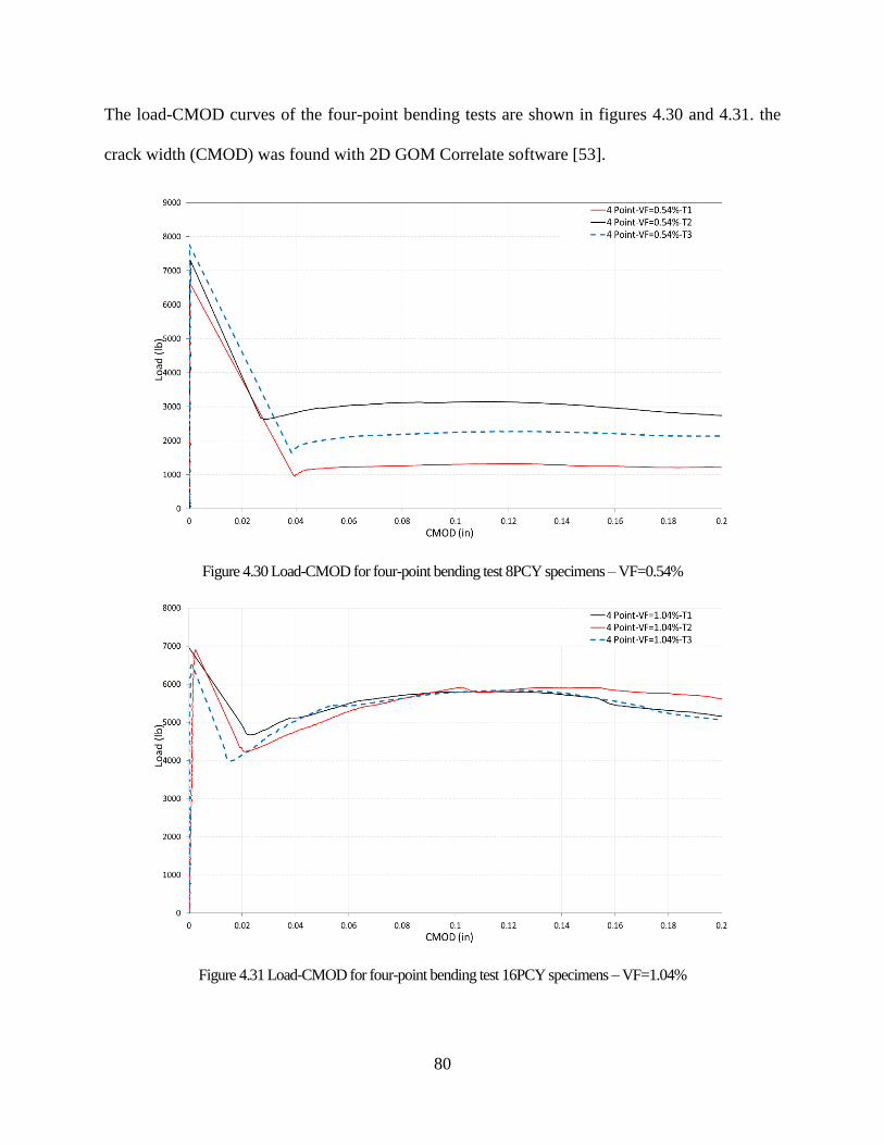
80
The load-CMOD curves of the four-point bending tests are shown in figures 4.30 and 4.31. the
crack width (CMOD) was found with 2D GOM Correlate software [53].
Figure 4.30 Load-CMOD for four-point bending test 8PCY specimens – VF=0.54%
Figure 4.31 Load-CMOD for four-point bending test 16PCY specimens – VF=1.04%
81
4.1.4.Conclusions of the crack width measurement tests
The crack width measurement was performed for two different type of bending tests. The results
of these tests can be used to verify the crack width measurement procedure with FE models which
will be described in chapter 4 of this research. DIC method was successfully adopted and calibrated
to measure the crack width and has been proven to be a reliable method to do this. Since the
position of the crack in four-point bending tests is not predefined by the notch, they will be a good
verification for the performance of FE crack width measurement method.
By using 1% volume fraction of synthetic fibers, it has been shown that the behavior of bending
specimens will be drastically change and the bridging effect will act to overcome the increasing of
crack width. The post-processing capability of the 2D DIC method makes it possible to find the
location of the crack from the last image and then calculate the deformation of the points across
the crack section from the beginning of the test.
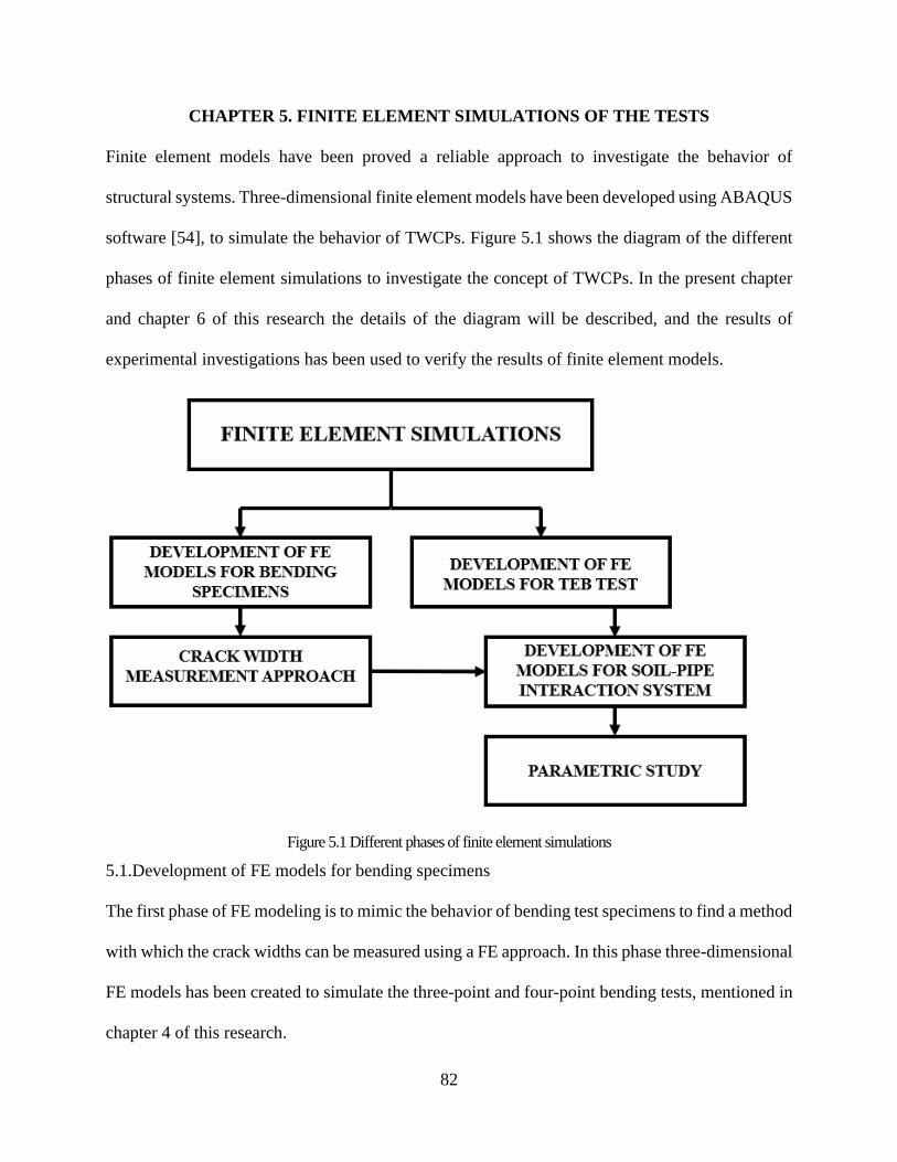
82
CHAPTER 5. FINITE ELEMENT SIMULATIONS OF THE TESTS
Finite element models have been proved a reliable approach to investigate the behavior of
structural systems. Three-dimensional finite element models have been developed using ABAQUS
software [54], to simulate the behavior of TWCPs. Figure 5.1 shows the diagram of the different
phases of finite element simulations to investigate the concept of TWCPs. In the present chapter
and chapter 6 of this research the details of the diagram will be described, and the results of
experimental investigations has been used to verify the results of finite element models.
Figure 5.1 Different phases of finite element simulations
5.1.Development of FE models for bending specimens
The first phase of FE modeling is to mimic the behavior of bending test specimens to find a method
with which the crack widths can be measured using a FE approach. In this phase three-dimensional
FE models has been created to simulate the three-point and four-point bending tests, mentioned in
chapter 4 of this research.
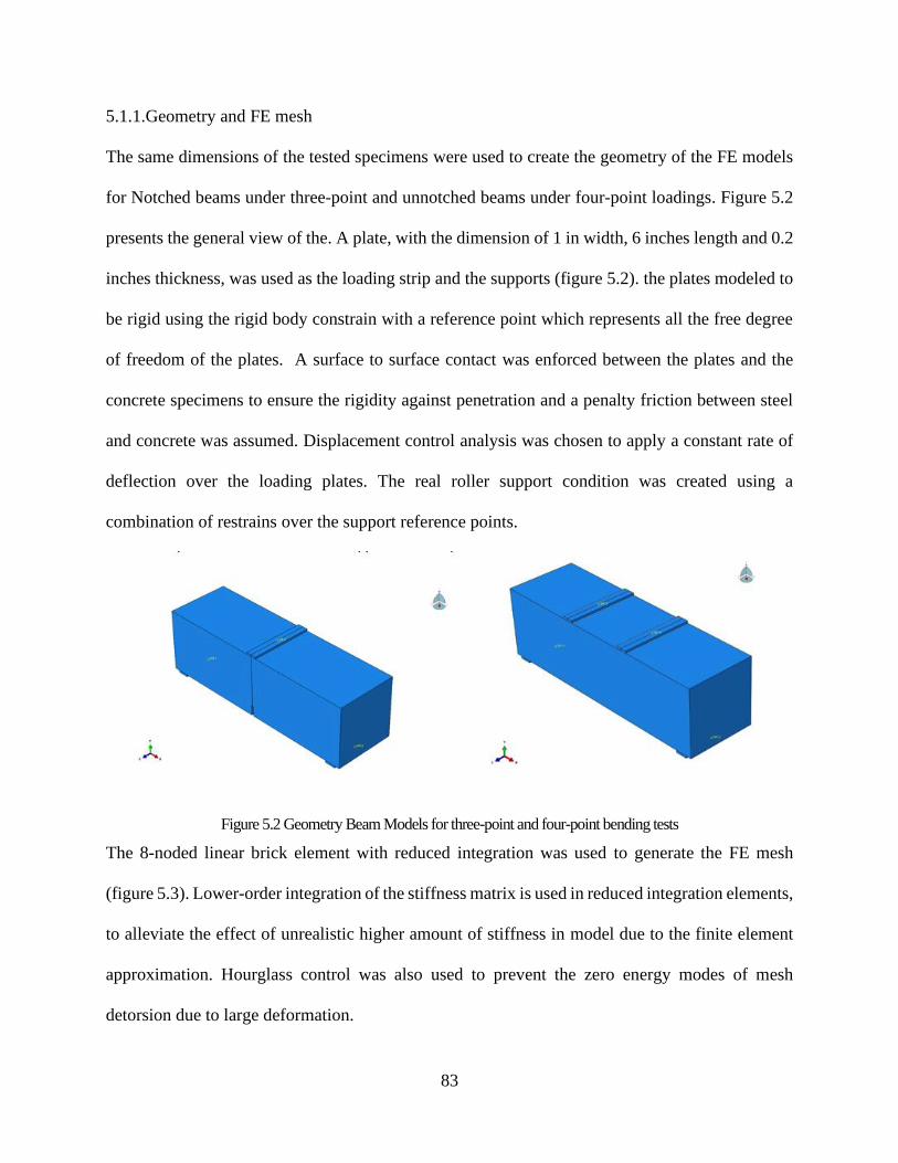
83
5.1.1.Geometry and FE mesh
The same dimensions of the tested specimens were used to create the geometry of the FE models
for Notched beams under three-point and unnotched beams under four-point loadings. Figure 5.2
presents the general view of the. A plate, with the dimension of 1 in width, 6 inches length and 0.2
inches thickness, was used as the loading strip and the supports (figure 5.2). the plates modeled to
be rigid using the rigid body constrain with a reference point which represents all the free degree
of freedom of the plates. A surface to surface contact was enforced between the plates and the
concrete specimens to ensure the rigidity against penetration and a penalty friction between steel
and concrete was assumed. Displacement control analysis was chosen to apply a constant rate of
deflection over the loading plates. The real roller support condition was created using a
combination of restrains over the support reference points.
Figure 5.2 Geometry Beam Models for three-point and four-point bending tests
The 8-noded linear brick element with reduced integration was used to generate the FE mesh
(figure 5.3). Lower-order integration of the stiffness matrix is used in reduced integration elements,
to alleviate the effect of unrealistic higher amount of stiffness in model due to the finite element
approximation. Hourglass control was also used to prevent the zero energy modes of mesh
detorsion due to large deformation.
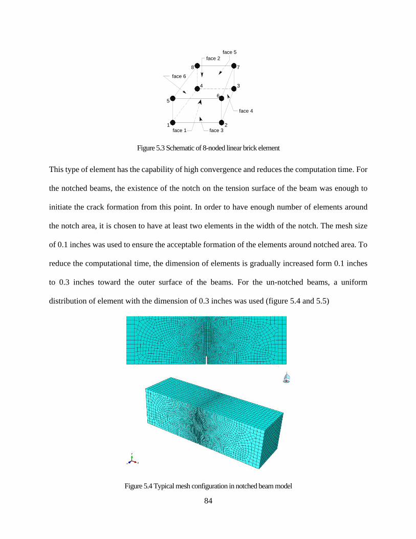
84
Figure 5.3 Schematic of 8-noded linear brick element
This type of element has the capability of high convergence and reduces the computation time. For
the notched beams, the existence of the notch on the tension surface of the beam was enough to
initiate the crack formation from this point. In order to have enough number of elements around
the notch area, it is chosen to have at least two elements in the width of the notch. The mesh size
of 0.1 inches was used to ensure the acceptable formation of the elements around notched area. To
reduce the computational time, the dimension of elements is gradually increased form 0.1 inches
to 0.3 inches toward the outer surface of the beams. For the un-notched beams, a uniform
distribution of element with the dimension of 0.3 inches was used (figure 5.4 and 5.5)
Figure 5.4 Typical mesh configuration in notched beam model
face 1 face 3
face 4
face 2
face 5
face 6
1
5
8 7
3
2
6
4
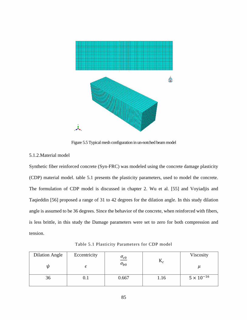
85
Figure 5.5 Typical mesh configuration in un-notched beam model
5.1.2.Material model
Synthetic fiber reinforced concrete (Syn-FRC) was modeled using the concrete damage plasticity
(CDP) material model. table 5.1 presents the plasticity parameters, used to model the concrete.
The formulation of CDP model is discussed in chapter 2. Wu et al. [55] and Voyiadjis and
Taqieddin [56] proposed a range of 31 to 42 degrees for the dilation angle. In this study dilation
angle is assumed to be 36 degrees. Since the behavior of the concrete, when reinforced with fibers,
is less brittle, in this study the Damage parameters were set to zero for both compression and
tension.
Table 5.1 Plasticity Parameters for CDP model
Dilation Angle
𝜓
Eccentricity
𝜖
𝜎𝑐0𝜎𝑏0
K𝑐 Viscosity
𝜇
36 0.1 0.667 1.16 5 × 10⁻¹⁶
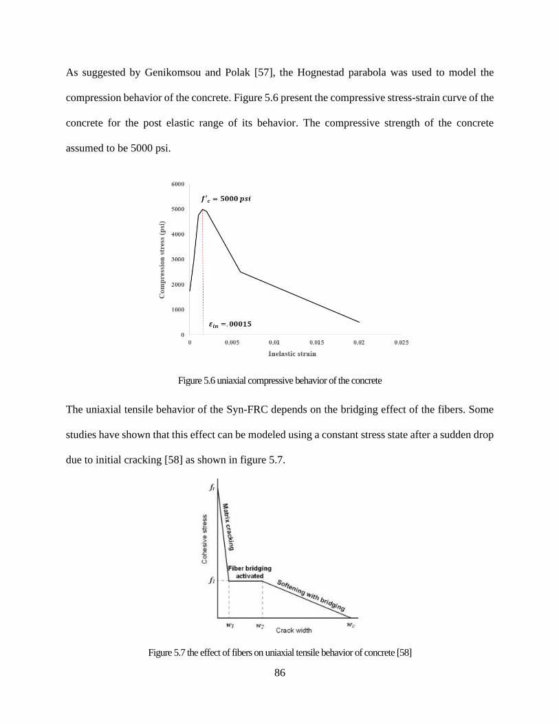
86
As suggested by Genikomsou and Polak [57], the Hognestad parabola was used to model the
compression behavior of the concrete. Figure 5.6 present the compressive stress-strain curve of the
concrete for the post elastic range of its behavior. The compressive strength of the concrete
assumed to be 5000 psi.
Figure 5.6 uniaxial compressive behavior of the concrete
The uniaxial tensile behavior of the Syn-FRC depends on the bridging effect of the fibers. Some
studies have shown that this effect can be modeled using a constant stress state after a sudden drop
due to initial cracking [58] as shown in figure 5.7.
Figure 5.7 the effect of fibers on uniaxial tensile behavior of concrete [58]
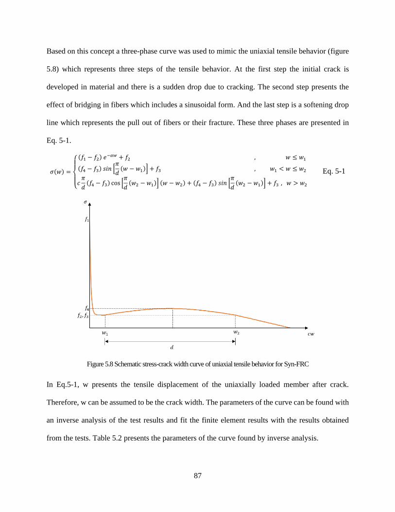
87
Based on this concept a three-phase curve was used to mimic the uniaxial tensile behavior (figure
5.8) which represents three steps of the tensile behavior. At the first step the initial crack is
developed in material and there is a sudden drop due to cracking. The second step presents the
effect of bridging in fibers which includes a sinusoidal form. And the last step is a softening drop
line which represents the pull out of fibers or their fracture. These three phases are presented in
Eq. 5-1.
𝜎(𝑤) =
{
(𝑓1 − 𝑓2) 𝑒
−𝛼𝑤 + 𝑓2 , 𝑤 ≤ 𝑤1
(𝑓4 − 𝑓3) 𝑠𝑖𝑛 [𝜋
𝑑(𝑤 − 𝑤1)] + 𝑓3 , 𝑤1 < 𝑤 ≤ 𝑤2
𝑐𝜋
𝑑(𝑓4 − 𝑓3) cos [
𝜋
𝑑(𝑤2 − 𝑤1)] (𝑤 − 𝑤2) + (𝑓4 − 𝑓3) 𝑠𝑖𝑛 [
𝜋
𝑑(𝑤2 − 𝑤1)] + 𝑓3 , 𝑤 > 𝑤2
Eq. 5-1
Figure 5.8 Schematic stress-crack width curve of uniaxial tensile behavior for Syn-FRC
In Eq.5-1, w presents the tensile displacement of the uniaxially loaded member after crack.
Therefore, w can be assumed to be the crack width. The parameters of the curve can be found with
an inverse analysis of the test results and fit the finite element results with the results obtained
from the tests. Table 5.2 presents the parameters of the curve found by inverse analysis.
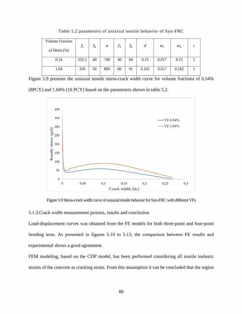
88
Table 5.2 parameters of uniaxial tensile behavior of Syn-FRC
Volume Fraction
of fibers (%)
𝑓1 𝑓2 𝛼 𝑓3 𝑓4 𝑑 𝑤1 𝑤2 𝑐
0.54 332.5 40 740 40 60 0.15 0.017 0.15 1
1.04 359 50 800 60 91 0.165 0.017 0.182 1
Figure 5.9 presents the uniaxial tensile stress-crack width curve for volume fractions of 0.54%
(8PCY) and 1.04% (16 PCY) based on the parameters shown in table 5.2.
Figure 5.9 Stress-crack width curve of uniaxial tensile behavior for Syn-FRC with different VFs
5.1.3.Crack width measurement process, results and conclusion
Load-displacement curves was obtained from the FE models for both three-point and four-point
bending tests. As presented in figures 5.10 to 5.13, the comparison between FE results and
experimental shows a good agreement.
FEM modeling, based on the CDP model, has been performed considering all tensile inelastic
strains of the concrete as cracking strain. From this assumption it can be concluded that the region
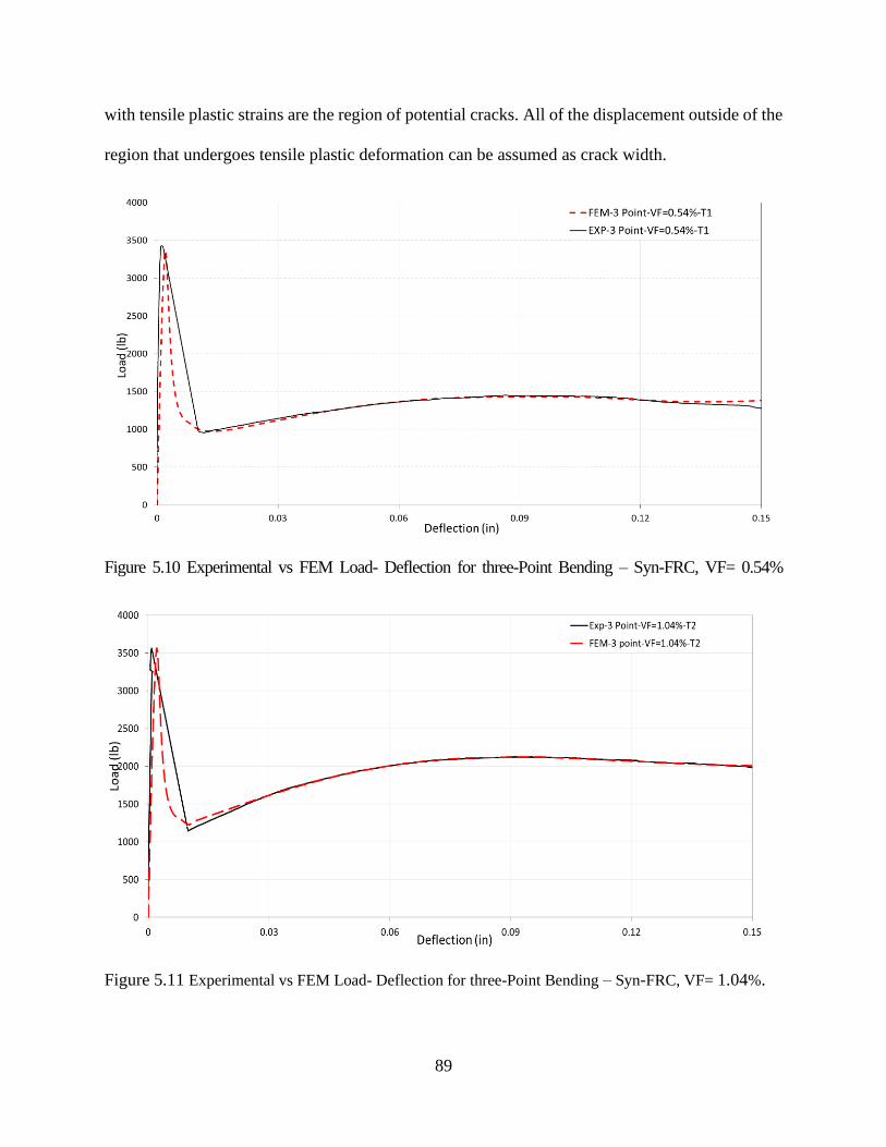
89
with tensile plastic strains are the region of potential cracks. All of the displacement outside of the
region that undergoes tensile plastic deformation can be assumed as crack width.
Figure 5.10 Experimental vs FEM Load- Deflection for three-Point Bending – Syn-FRC, VF= 0.54%
Figure 5.11 Experimental vs FEM Load- Deflection for three-Point Bending – Syn-FRC, VF= 1.04%.
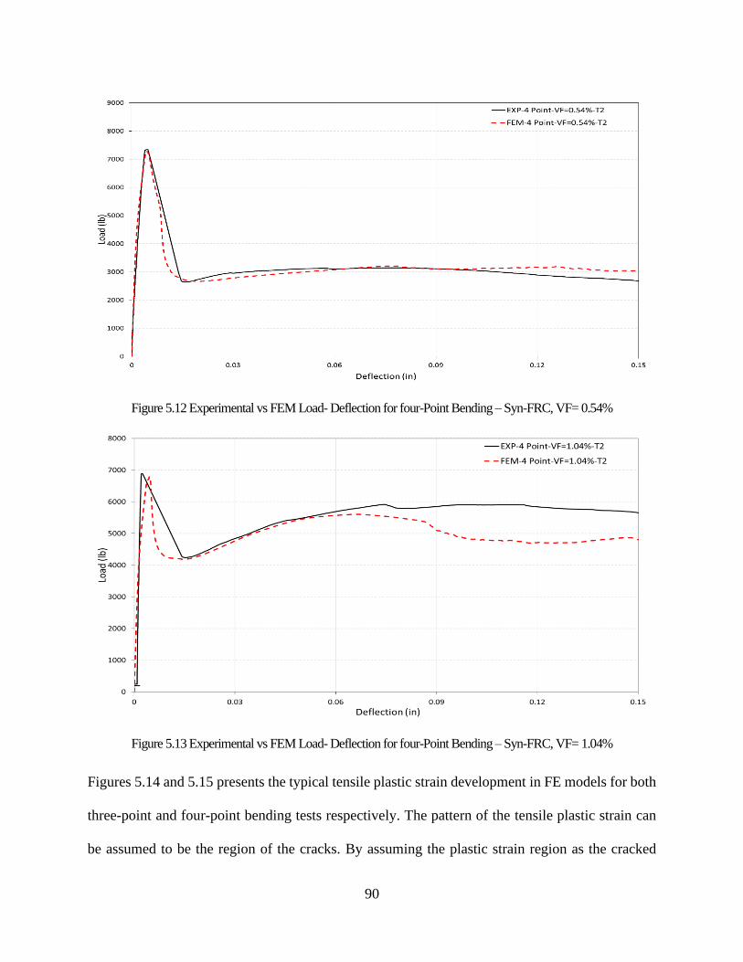
90
Figure 5.12 Experimental vs FEM Load- Deflection for four-Point Bending – Syn-FRC, VF= 0.54%
Figure 5.13 Experimental vs FEM Load- Deflection for four-Point Bending – Syn-FRC, VF= 1.04%
Figures 5.14 and 5.15 presents the typical tensile plastic strain development in FE models for both
three-point and four-point bending tests respectively. The pattern of the tensile plastic strain can
be assumed to be the region of the cracks. By assuming the plastic strain region as the cracked
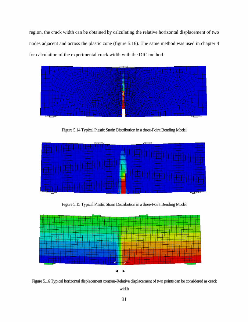
91
region, the crack width can be obtained by calculating the relative horizontal displacement of two
nodes adjacent and across the plastic zone (figure 5.16). The same method was used in chapter 4
for calculation of the experimental crack width with the DIC method.
Figure 5.14 Typical Plastic Strain Distribution in a three-Point Bending Model
Figure 5.15 Typical Plastic Strain Distribution in a three-Point Bending Model
Figure 5.16 Typical horizontal displacement contour-Relative displacement of two points can be considered as crack
width
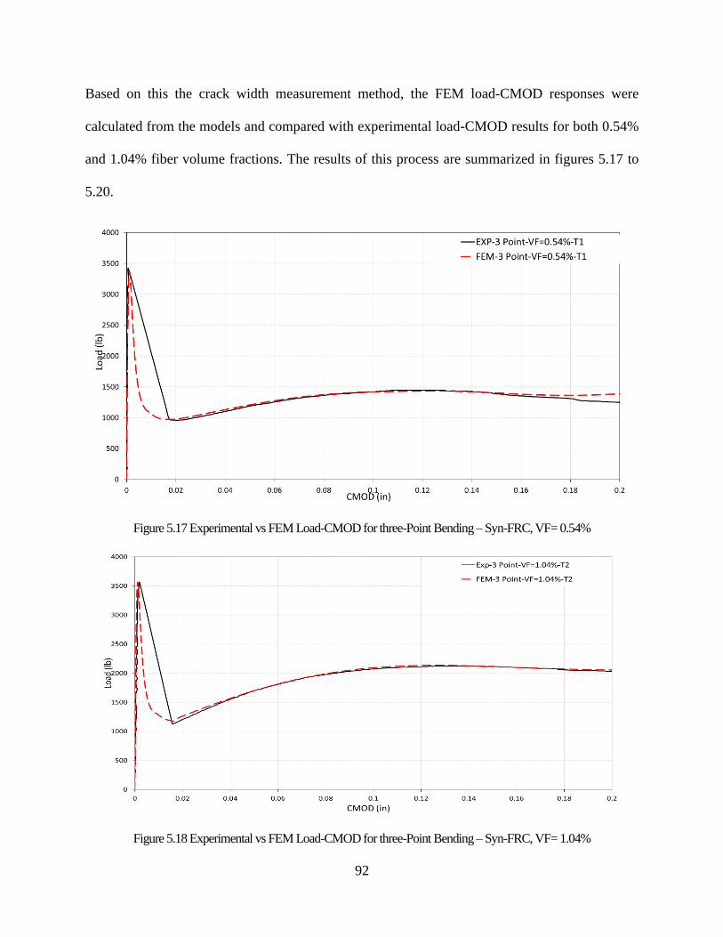
92
Based on this the crack width measurement method, the FEM load-CMOD responses were
calculated from the models and compared with experimental load-CMOD results for both 0.54%
and 1.04% fiber volume fractions. The results of this process are summarized in figures 5.17 to
5.20.
Figure 5.17 Experimental vs FEM Load-CMOD for three-Point Bending – Syn-FRC, VF= 0.54%
Figure 5.18 Experimental vs FEM Load-CMOD for three-Point Bending – Syn-FRC, VF= 1.04%
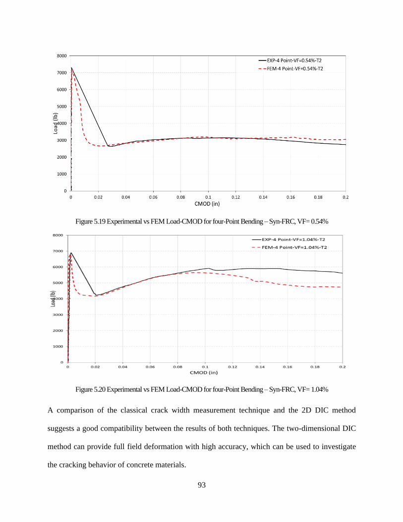
93
Figure 5.19 Experimental vs FEM Load-CMOD for four-Point Bending – Syn-FRC, VF= 0.54%
Figure 5.20 Experimental vs FEM Load-CMOD for four-Point Bending – Syn-FRC, VF= 1.04%
A comparison of the classical crack width measurement technique and the 2D DIC method
suggests a good compatibility between the results of both techniques. The two-dimensional DIC
method can provide full field deformation with high accuracy, which can be used to investigate
the cracking behavior of concrete materials.

94
Implementation of the suggested tensile-softening behavior, in terms of stress-crack width into
three-dimensional nonlinear FEM modeling based on the concrete damage plasticity, provided a
good approximation of the synthetic FRC material behavior. Numerical crack width was
calculated, considering the relative displacement of the nodes across the plastic strain band. This
band was assumed to correspond to the crack surface. The FE results were in good agreement with
the experimental results of load-crack width for beams under three-point and four-point bending.
The proposed method of crack measurement using FEM can be used as a tool to measure the crack
width of any other structural member.
5.2.Development of FE models for Three-Edge Bearing (TEB) tests
The second phase of FE simulations was to create models to mimic the behavior of TWCPs under
TEB test. This phase helped to find the bests tensile stress softening curve for the Syn-FRC, used
in industry. As mentioned in chapter 3, the TWCPs were created using a dry mixed concrete using
a packerhead equipment. The effect of industrial process on the material property of the Syn-FRC
was evaluated in this phase as well as the capability of FE modeling to mimic the TEB tests.
5.2.1.Geometry and FE mesh
Figure 5.21 presents the geometry of FE model for a typical TEB test. Because of the symmetricity
of the model along the length of the pipe, TWCP was modeled in a 12 in. length to reduce the
number of elements needed for the analysis and corresponding time. In a typica industrial practice
the three circles of circumferential reinforcement are used per foot of the pipe length. The distance
between the circles is 3.0 in. (figure 5.21). the Area of circumferential reinforcement is given in
table 5.3. supports were modeled using two robber pads with 1.5 in. width and 2.0 in length
rectangular cross section. the loading plate assumed to be a rigid beam with the rectangular cross
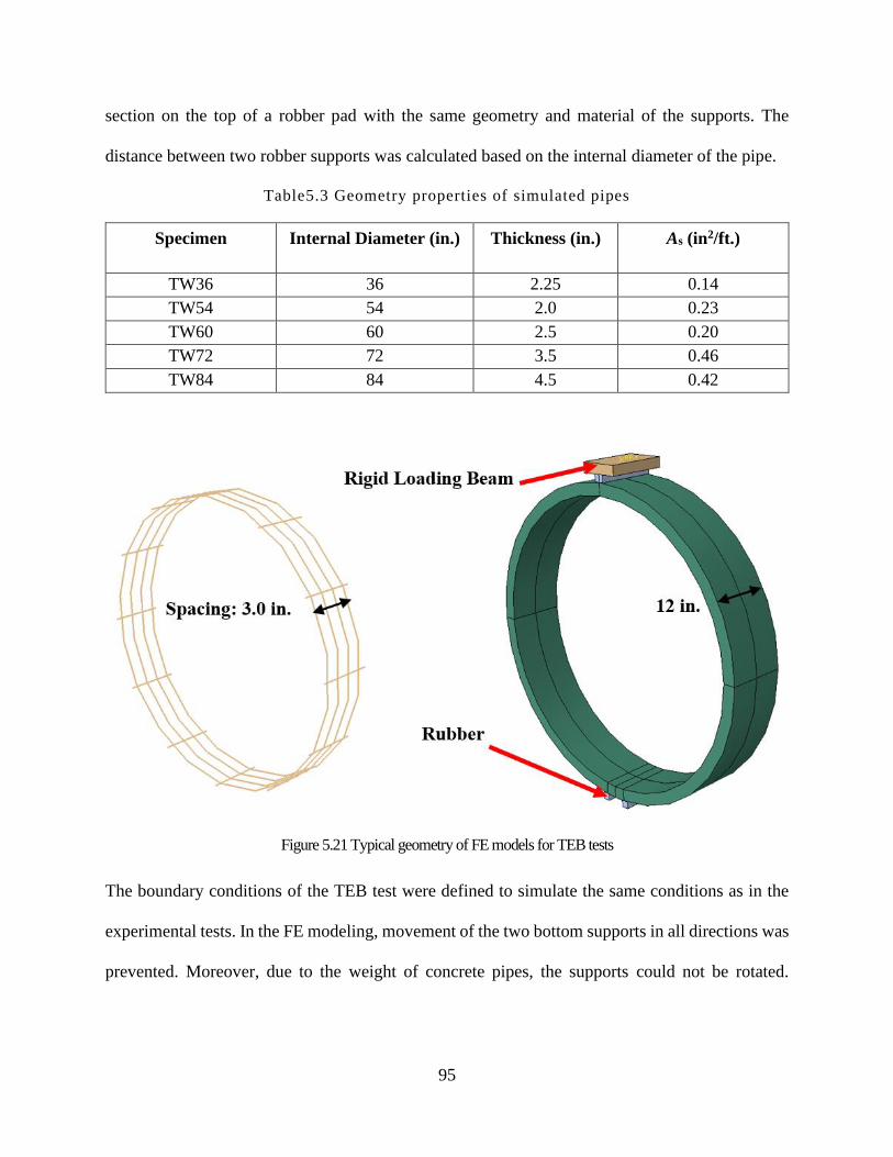
95
section on the top of a robber pad with the same geometry and material of the supports. The
distance between two robber supports was calculated based on the internal diameter of the pipe.
Table5.3 Geometry properties of simulated pipes
Specimen Internal Diameter (in.) Thickness (in.) As (in2/ft.)
TW36 36 2.25 0.14
TW54 54 2.0 0.23
TW60 60 2.5 0.20
TW72 72 3.5 0.46
TW84 84 4.5 0.42
Figure 5.21 Typical geometry of FE models for TEB tests
The boundary conditions of the TEB test were defined to simulate the same conditions as in the
experimental tests. In the FE modeling, movement of the two bottom supports in all directions was
prevented. Moreover, due to the weight of concrete pipes, the supports could not be rotated.
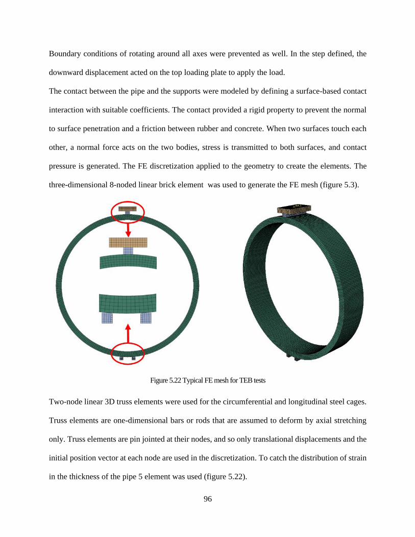
96
Boundary conditions of rotating around all axes were prevented as well. In the step defined, the
downward displacement acted on the top loading plate to apply the load.
The contact between the pipe and the supports were modeled by defining a surface-based contact
interaction with suitable coefficients. The contact provided a rigid property to prevent the normal
to surface penetration and a friction between rubber and concrete. When two surfaces touch each
other, a normal force acts on the two bodies, stress is transmitted to both surfaces, and contact
pressure is generated. The FE discretization applied to the geometry to create the elements. The
three-dimensional 8-noded linear brick element was used to generate the FE mesh (figure 5.3).
Figure 5.22 Typical FE mesh for TEB tests
Two-node linear 3D truss elements were used for the circumferential and longitudinal steel cages.
Truss elements are one-dimensional bars or rods that are assumed to deform by axial stretching
only. Truss elements are pin jointed at their nodes, and so only translational displacements and the
initial position vector at each node are used in the discretization. To catch the distribution of strain
in the thickness of the pipe 5 element was used (figure 5.22).
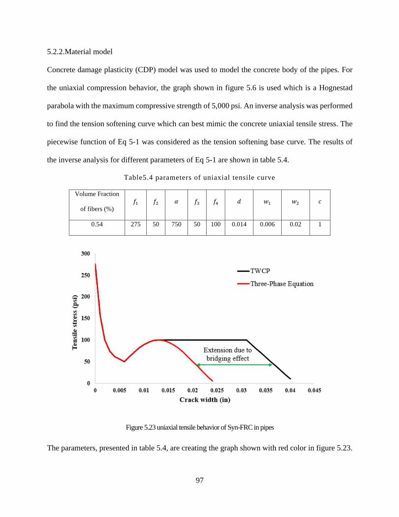
97
5.2.2.Material model
Concrete damage plasticity (CDP) model was used to model the concrete body of the pipes. For
the uniaxial compression behavior, the graph shown in figure 5.6 is used which is a Hognestad
parabola with the maximum compressive strength of 5,000 psi. An inverse analysis was performed
to find the tension softening curve which can best mimic the concrete uniaxial tensile stress. The
piecewise function of Eq 5-1 was considered as the tension softening base curve. The results of
the inverse analysis for different parameters of Eq 5-1 are shown in table 5.4.
Table5.4 parameters of uniaxial tensile curve
Volume Fraction
of fibers (%)
𝑓1 𝑓2 𝛼 𝑓3 𝑓4 𝑑 𝑤1 𝑤2 𝑐
0.54 275 50 750 50 100 0.014 0.006 0.02 1
Figure 5.23 uniaxial tensile behavior of Syn-FRC in pipes
The parameters, presented in table 5.4, are creating the graph shown with red color in figure 5.23.
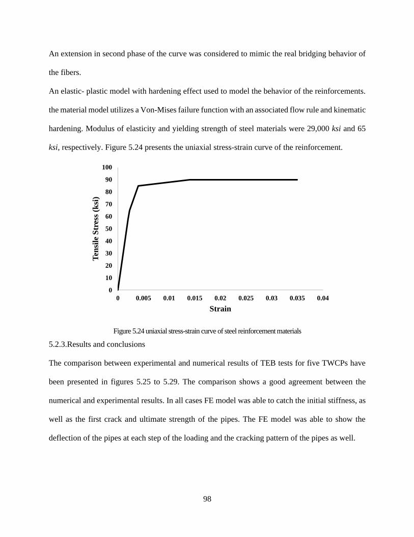
98
An extension in second phase of the curve was considered to mimic the real bridging behavior of
the fibers.
An elastic- plastic model with hardening effect used to model the behavior of the reinforcements.
the material model utilizes a Von-Mises failure function with an associated flow rule and kinematic
hardening. Modulus of elasticity and yielding strength of steel materials were 29,000 ksi and 65
ksi, respectively. Figure 5.24 presents the uniaxial stress-strain curve of the reinforcement.
Figure 5.24 uniaxial stress-strain curve of steel reinforcement materials
5.2.3.Results and conclusions
The comparison between experimental and numerical results of TEB tests for five TWCPs have
been presented in figures 5.25 to 5.29. The comparison shows a good agreement between the
numerical and experimental results. In all cases FE model was able to catch the initial stiffness, as
well as the first crack and ultimate strength of the pipes. The FE model was able to show the
deflection of the pipes at each step of the loading and the cracking pattern of the pipes as well.
0
10
20
30
40
50
60
70
80
90
100
0 0.005 0.01 0.015 0.02 0.025 0.03 0.035 0.04
Ten
sile
Str
ess
(ksi
)
Strain
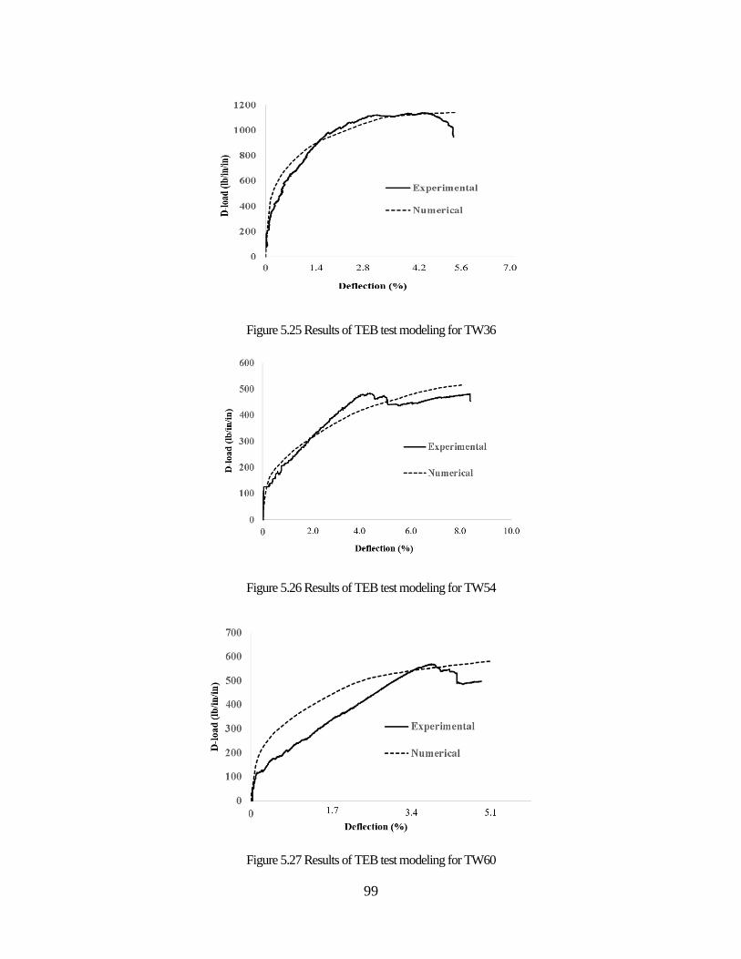
99
Figure 5.25 Results of TEB test modeling for TW36
Figure 5.26 Results of TEB test modeling for TW54
Figure 5.27 Results of TEB test modeling for TW60
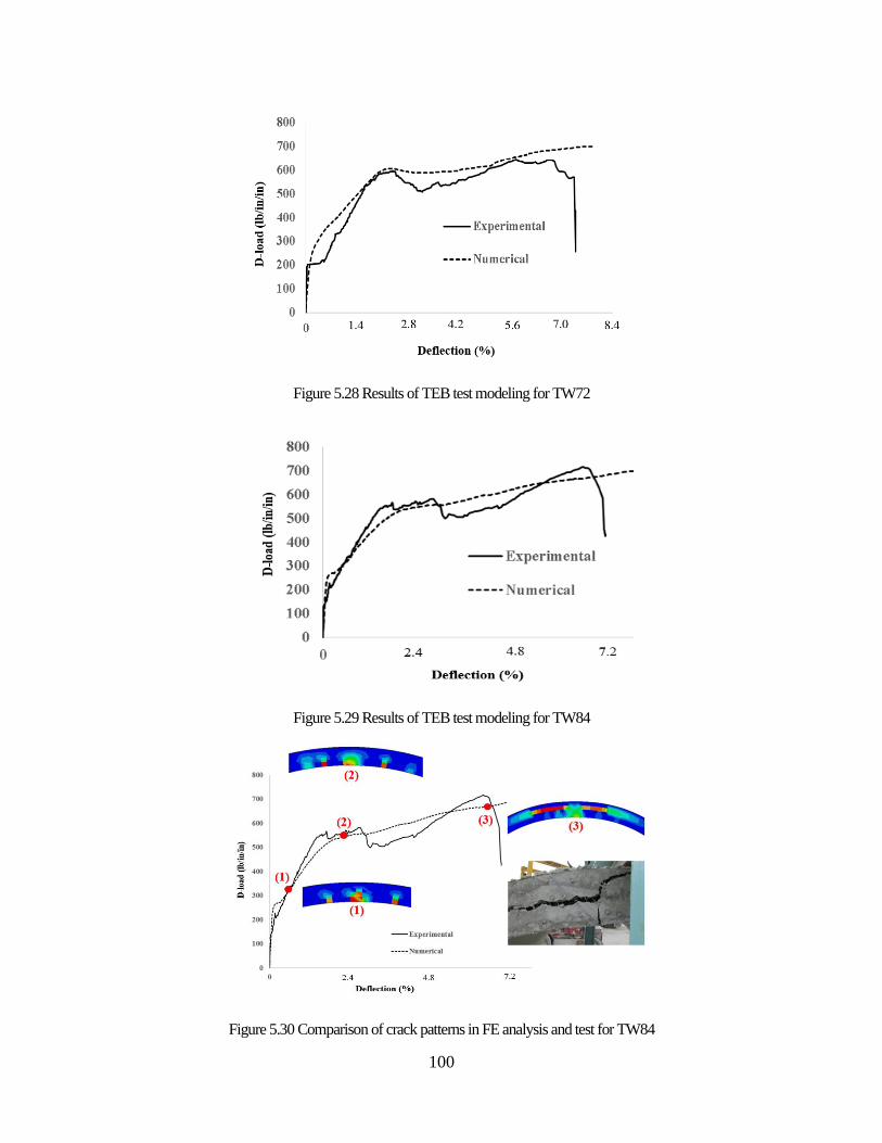
100
Figure 5.28 Results of TEB test modeling for TW72
Figure 5.29 Results of TEB test modeling for TW84
Figure 5.30 Comparison of crack patterns in FE analysis and test for TW84
101
Figure 5.30 presents the development of cracks in the crown of a TWCP of 84 in. diameter. The
crack pattern can be obtained by looking at plastic tensile strain contours. At different stages of
loading the development of cracks have been shown and it will reach to the final stage (number 3
in figure 5.30) in which a diagonal tensile crack has been developed. The experimental crack
pattern at the final stage has a good agreement with the results of FE models. The uniaxial tensile
behavior of the concrete, shown in figure 5.23, have been proved to be useful for FE modeling of
TWCPs, produced with industrial equipment, which was the main goal of second phase of FE
simulations (TEB tests simulations)
5.3.Summary and conclusions
Different phases of the FE simulations are described in figure 5.1 two phases of which has been
addressed in chapter 5. The first phase was to develop a FE model for three and four-point bending
tests to show the capability of FE analysis to simulate the behavior of the Syn-FRC. A modification
of uniaxial tensile behavior of the concrete using CDP material model was used to consider the
effect of fiber bridging and it has been proved to be capable of simulating the experimental results.
Using the tensile plastic strain field from FE results a method is introduced to calculate the crack
width in specimens and the results of this calculations shows a good agreement with experimental
crack width measurements using DIC method. The proposed FE crack width measurement method
will be used in chapter 6 to measure the crack width of TWCPs in interaction and under the loads
of the soil as the third phase of FE simulations.
The second phase was to develop a FE model to mimic the behavior of TWCPs under TEB tests.
In this phase a modification of uniaxial tensile curve was introduced considering the model,
proposed in first phase of FE analysis. The results show a good agreement with the tests both in
load-displacement curves and the crack patterns.
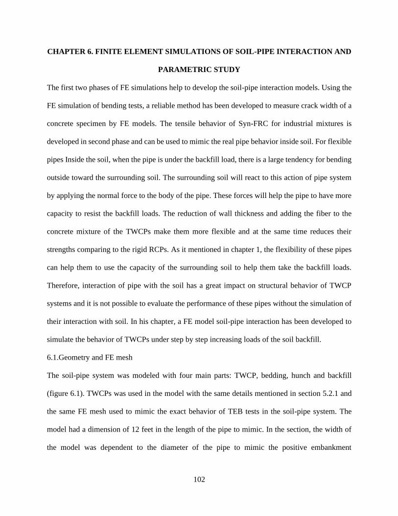
102
CHAPTER 6. FINITE ELEMENT SIMULATIONS OF SOIL-PIPE INTERACTION AND
PARAMETRIC STUDY
The first two phases of FE simulations help to develop the soil-pipe interaction models. Using the
FE simulation of bending tests, a reliable method has been developed to measure crack width of a
concrete specimen by FE models. The tensile behavior of Syn-FRC for industrial mixtures is
developed in second phase and can be used to mimic the real pipe behavior inside soil. For flexible
pipes Inside the soil, when the pipe is under the backfill load, there is a large tendency for bending
outside toward the surrounding soil. The surrounding soil will react to this action of pipe system
by applying the normal force to the body of the pipe. These forces will help the pipe to have more
capacity to resist the backfill loads. The reduction of wall thickness and adding the fiber to the
concrete mixture of the TWCPs make them more flexible and at the same time reduces their
strengths comparing to the rigid RCPs. As it mentioned in chapter 1, the flexibility of these pipes
can help them to use the capacity of the surrounding soil to help them take the backfill loads.
Therefore, interaction of pipe with the soil has a great impact on structural behavior of TWCP
systems and it is not possible to evaluate the performance of these pipes without the simulation of
their interaction with soil. In his chapter, a FE model soil-pipe interaction has been developed to
simulate the behavior of TWCPs under step by step increasing loads of the soil backfill.
6.1.Geometry and FE mesh
The soil-pipe system was modeled with four main parts: TWCP, bedding, hunch and backfill
(figure 6.1). TWCPs was used in the model with the same details mentioned in section 5.2.1 and
the same FE mesh used to mimic the exact behavior of TEB tests in the soil-pipe system. The
model had a dimension of 12 feet in the length of the pipe to mimic. In the section, the width of
the model was dependent to the diameter of the pipe to mimic the positive embankment
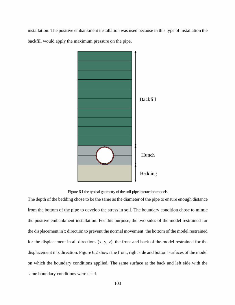
103
installation. The positive embankment installation was used because in this type of installation the
backfill would apply the maximum pressure on the pipe.
Figure 6.1 the typical geometry of the soil-pipe interaction models
The depth of the bedding chose to be the same as the diameter of the pipe to ensure enough distance
from the bottom of the pipe to develop the stress in soil. The boundary condition chose to mimic
the positive embankment installation. For this purpose, the two sides of the model restrained for
the displacement in x direction to prevent the normal movement. the bottom of the model restrained
for the displacement in all directions (x, y, z). the front and back of the model restrained for the
displacement in z direction. Figure 6.2 shows the front, right side and bottom surfaces of the model
on which the boundary conditions applied. The same surface at the back and left side with the
same boundary conditions were used.
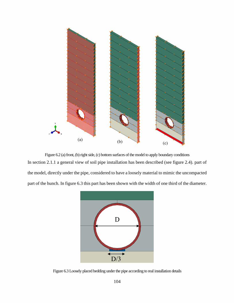
104
Figure 6.2 (a) front, (b) right side, (c) bottom surfaces of the model to apply boundary conditions
In section 2.1.1 a general view of soil pipe installation has been described (see figure 2.4). part of
the model, directly under the pipe, considered to have a loosely material to mimic the uncompacted
part of the hunch. In figure 6.3 this part has been shown with the width of one third of the diameter.
Figure 6.3 Loosely placed bedding under the pipe according to real installation details
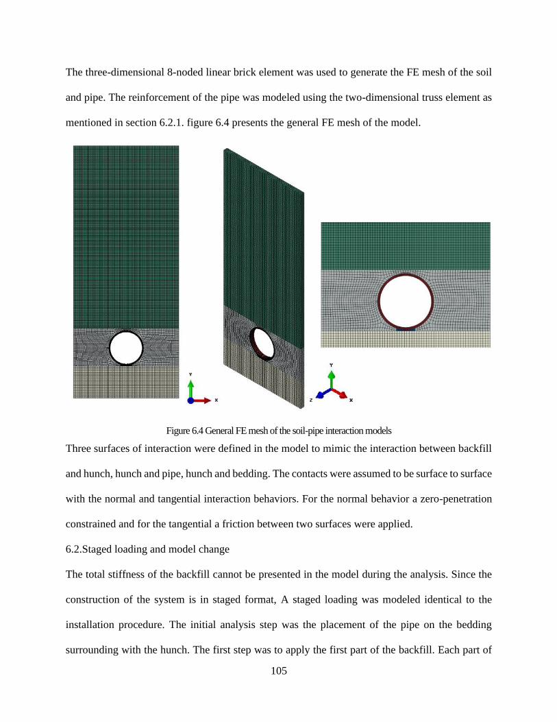
105
The three-dimensional 8-noded linear brick element was used to generate the FE mesh of the soil
and pipe. The reinforcement of the pipe was modeled using the two-dimensional truss element as
mentioned in section 6.2.1. figure 6.4 presents the general FE mesh of the model.
Figure 6.4 General FE mesh of the soil-pipe interaction models
Three surfaces of interaction were defined in the model to mimic the interaction between backfill
and hunch, hunch and pipe, hunch and bedding. The contacts were assumed to be surface to surface
with the normal and tangential interaction behaviors. For the normal behavior a zero-penetration
constrained and for the tangential a friction between two surfaces were applied.
6.2.Staged loading and model change
The total stiffness of the backfill cannot be presented in the model during the analysis. Since the
construction of the system is in staged format, A staged loading was modeled identical to the
installation procedure. The initial analysis step was the placement of the pipe on the bedding
surrounding with the hunch. The first step was to apply the first part of the backfill. Each part of
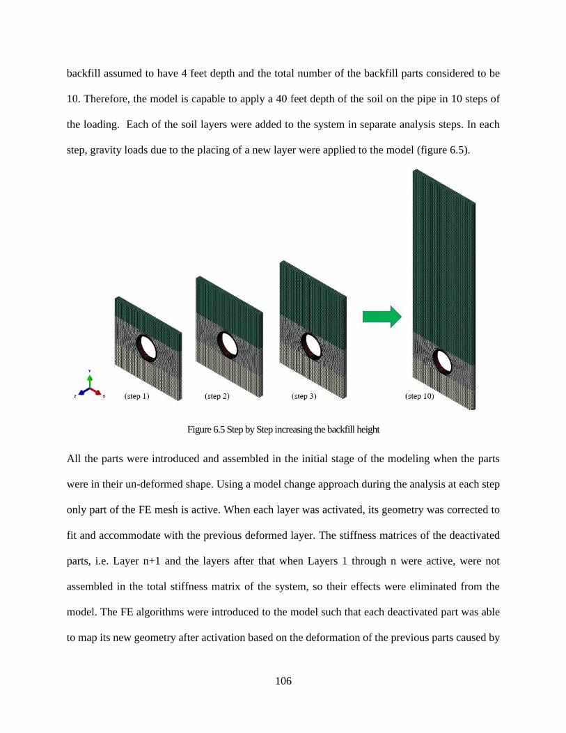
106
backfill assumed to have 4 feet depth and the total number of the backfill parts considered to be
10. Therefore, the model is capable to apply a 40 feet depth of the soil on the pipe in 10 steps of
the loading. Each of the soil layers were added to the system in separate analysis steps. In each
step, gravity loads due to the placing of a new layer were applied to the model (figure 6.5).
Figure 6.5 Step by Step increasing the backfill height
All the parts were introduced and assembled in the initial stage of the modeling when the parts
were in their un-deformed shape. Using a model change approach during the analysis at each step
only part of the FE mesh is active. When each layer was activated, its geometry was corrected to
fit and accommodate with the previous deformed layer. The stiffness matrices of the deactivated
parts, i.e. Layer n+1 and the layers after that when Layers 1 through n were active, were not
assembled in the total stiffness matrix of the system, so their effects were eliminated from the
model. The FE algorithms were introduced to the model such that each deactivated part was able
to map its new geometry after activation based on the deformation of the previous parts caused by
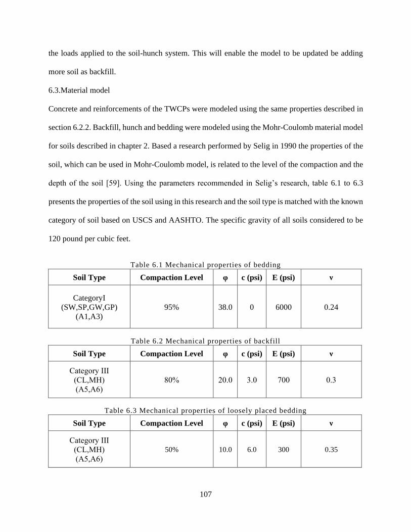
107
the loads applied to the soil-hunch system. This will enable the model to be updated be adding
more soil as backfill.
6.3.Material model
Concrete and reinforcements of the TWCPs were modeled using the same properties described in
section 6.2.2. Backfill, hunch and bedding were modeled using the Mohr-Coulomb material model
for soils described in chapter 2. Based a research performed by Selig in 1990 the properties of the
soil, which can be used in Mohr-Coulomb model, is related to the level of the compaction and the
depth of the soil [59]. Using the parameters recommended in Selig’s research, table 6.1 to 6.3
presents the properties of the soil using in this research and the soil type is matched with the known
category of soil based on USCS and AASHTO. The specific gravity of all soils considered to be
120 pound per cubic feet.
Table 6.1 Mechanical properties of bedding
Soil Type Compaction Level φ c (psi) E (psi) ν
CategoryI
(SW,SP,GW,GP)
(A1,A3)
95% 38.0 0 6000 0.24
Table 6.2 Mechanical properties of backfill
Soil Type Compaction Level φ c (psi) E (psi) ν
Category III
(CL,MH)
(A5,A6)
80% 20.0 3.0 700 0.3
Table 6.3 Mechanical properties of loosely placed bedding
Soil Type Compaction Level φ c (psi) E (psi) ν
Category III
(CL,MH)
(A5,A6)
50% 10.0 6.0 300 0.35
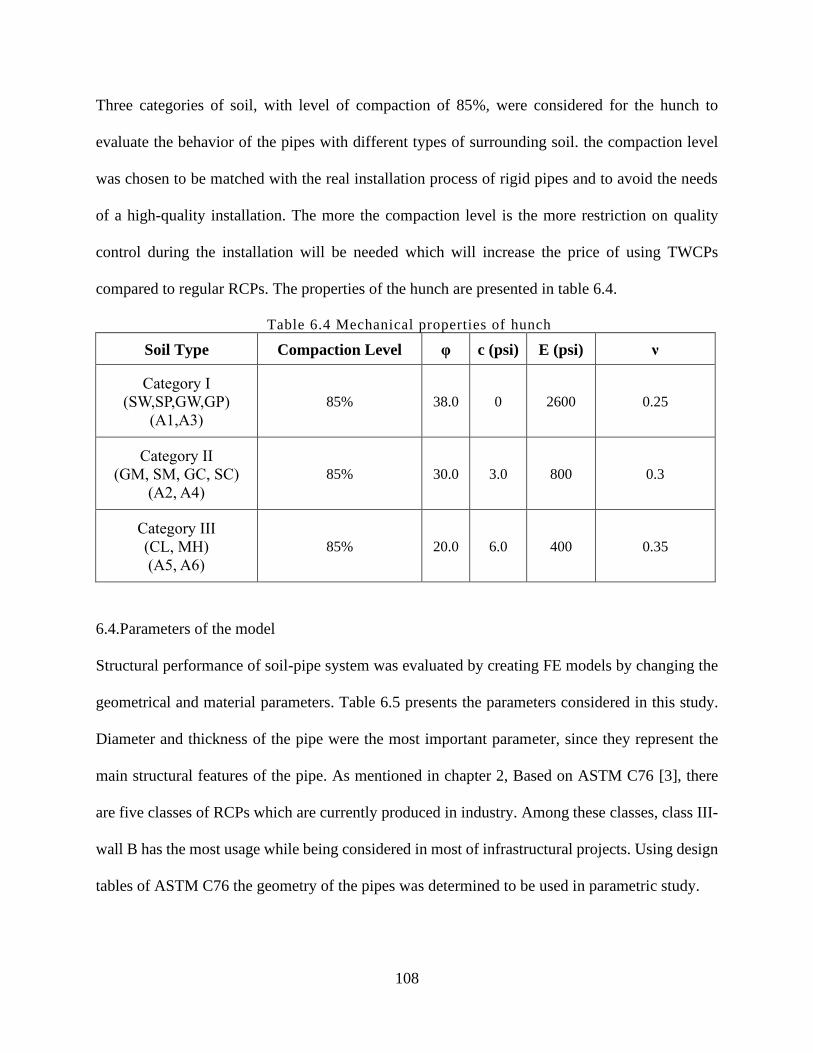
108
Three categories of soil, with level of compaction of 85%, were considered for the hunch to
evaluate the behavior of the pipes with different types of surrounding soil. the compaction level
was chosen to be matched with the real installation process of rigid pipes and to avoid the needs
of a high-quality installation. The more the compaction level is the more restriction on quality
control during the installation will be needed which will increase the price of using TWCPs
compared to regular RCPs. The properties of the hunch are presented in table 6.4.
Table 6.4 Mechanical properties of hunch
Soil Type Compaction Level φ c (psi) E (psi) ν
Category I
(SW,SP,GW,GP)
(A1,A3)
85% 38.0 0 2600 0.25
Category II
(GM, SM, GC, SC)
(A2, A4)
85% 30.0 3.0 800 0.3
Category III
(CL, MH)
(A5, A6)
85% 20.0 6.0 400 0.35
6.4.Parameters of the model
Structural performance of soil-pipe system was evaluated by creating FE models by changing the
geometrical and material parameters. Table 6.5 presents the parameters considered in this study.
Diameter and thickness of the pipe were the most important parameter, since they represent the
main structural features of the pipe. As mentioned in chapter 2, Based on ASTM C76 [3], there
are five classes of RCPs which are currently produced in industry. Among these classes, class III-
wall B has the most usage while being considered in most of infrastructural projects. Using design
tables of ASTM C76 the geometry of the pipes was determined to be used in parametric study.
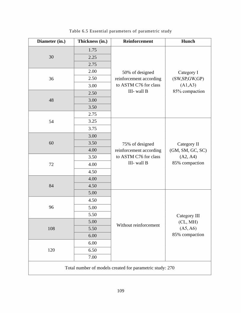
109
Table 6.5 Essential parameters of parametric study
Diameter (in.) Thickness (in.) Reinforcement Hunch
30
1.75
50% of designed
reinforcement according
to ASTM C76 for class
III- wall B
Category I
(SW,SP,GW,GP)
(A1,A3)
85% compaction
2.25
2.75
36
2.00
2.50
3.00
48
2.50
3.00
3.50
54
2.75
3.25
75% of designed
reinforcement according
to ASTM C76 for class
III- wall B
Category II
(GM, SM, GC, SC)
(A2, A4)
85% compaction
3.75
60
3.00
3.50
4.00
72
3.50
4.00
4.50
84
4.00
4.50
5.00
Without reinforcement
Category III
(CL, MH)
(A5, A6)
85% compaction
96
4.50
5.00
5.50
108
5.00
5.50
6.00
120
6.00
6.50
7.00
Total number of models created for parametric study: 270
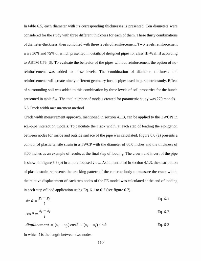
110
In table 6.5, each diameter with its corresponding thicknesses is presented. Ten diameters were
considered for the study with three different thickness for each of them. These thirty combinations
of diameter-thickness, then combined with three levels of reinforcement. Two levels reinforcement
were 50% and 75% of which presented in details of designed pipes for class III-Wall B according
to ASTM C76 [3]. To evaluate the behavior of the pipes without reinforcement the option of no-
reinforcement was added to these levels. The combination of diameter, thickness and
reinforcements will create ninety different geometry for the pipes used in parametric study. Effect
of surrounding soil was added to this combination by three levels of soil properties for the hunch
presented in table 6.4. The total number of models created for parametric study was 270 models.
6.5.Crack width measurement method
Crack width measurement approach, mentioned in section 4.1.3, can be applied to the TWCPs in
soil-pipe interaction models. To calculate the crack width, at each step of loading the elongation
between nodes for inside and outside surface of the pipe was calculated. Figure 6.6 (a) presents a
contour of plastic tensile strain in a TWCP with the diameter of 60.0 inches and the thickness of
3.00 inches as an example of results at the final step of loading. The crown and invert of the pipe
is shown in figure 6.6 (b) in a more focused view. As it mentioned in section 4.1.3, the distribution
of plastic strain represents the cracking pattern of the concrete body to measure the crack width,
the relative displacement of each two nodes of the FE model was calculated at the end of loading
in each step of load application using Eq. 6-1 to 6-3 (see figure 6.7).
sin 𝜃 =𝑦𝑖 − 𝑦𝑗
𝑙
Eq. 6-1
cos 𝜃 =𝑥𝑖 − 𝑥𝑗
𝑙
Eq. 6-2
𝑑𝑖𝑠𝑝𝑙𝑎𝑐𝑒𝑚𝑒𝑛𝑡 = (𝑢𝑖 − 𝑢𝑗) cos 𝜃 + (𝑣𝑖 − 𝑣𝑗) sin 𝜃 Eq. 6-3
In which 𝑙 is the length between two nodes
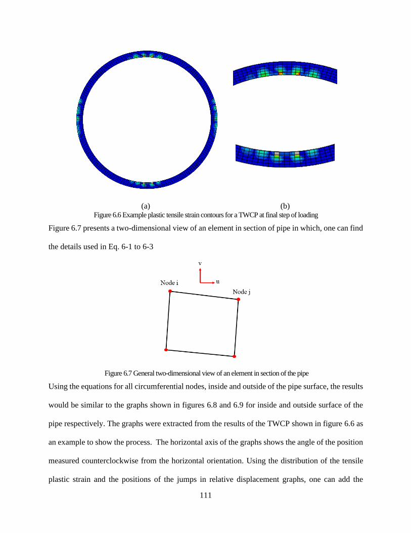
111
(a) (b) Figure 6.6 Example plastic tensile strain contours for a TWCP at final step of loading
Figure 6.7 presents a two-dimensional view of an element in section of pipe in which, one can find
the details used in Eq. 6-1 to 6-3
Figure 6.7 General two-dimensional view of an element in section of the pipe
Using the equations for all circumferential nodes, inside and outside of the pipe surface, the results
would be similar to the graphs shown in figures 6.8 and 6.9 for inside and outside surface of the
pipe respectively. The graphs were extracted from the results of the TWCP shown in figure 6.6 as
an example to show the process. The horizontal axis of the graphs shows the angle of the position
measured counterclockwise from the horizontal orientation. Using the distribution of the tensile
plastic strain and the positions of the jumps in relative displacement graphs, one can add the
112
relative displacements and find the crack widths. To do this, the relative displacements inside the
tensile plastic zone should be added.
Figure 6.8 Relative displacements of the nodes of inside pipe circumference
Figure 6.9 Relative displacements of the nodes of outside pipe circumference
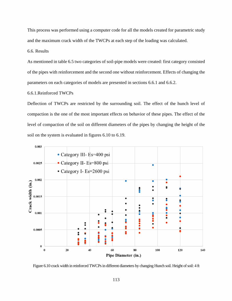
113
This process was performed using a computer code for all the models created for parametric study
and the maximum crack width of the TWCPs at each step of the loading was calculated.
6.6. Results
As mentioned in table 6.5 two categories of soil-pipe models were created: first category consisted
of the pipes with reinforcement and the second one without reinforcement. Effects of changing the
parameters on each categories of models are presented in sections 6.6.1 and 6.6.2.
6.6.1.Reinforced TWCPs
Deflection of TWCPs are restricted by the surrounding soil. The effect of the hunch level of
compaction is the one of the most important effects on behavior of these pipes. The effect of the
level of compaction of the soil on different diameters of the pipes by changing the height of the
soil on the system is evaluated in figures 6.10 to 6.19.
Figure 6.10 crack width in reinforced TWCPs in different diameters by changing Hunch soil. Height of soil: 4 ft
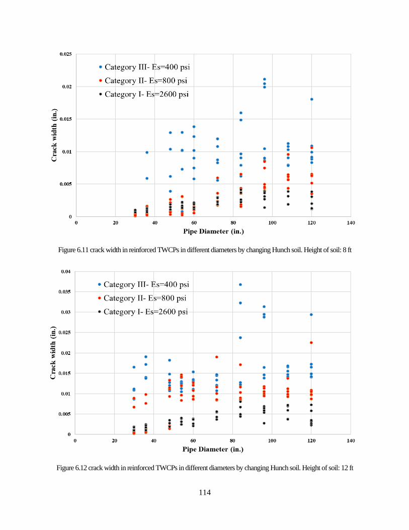
114
Figure 6.11 crack width in reinforced TWCPs in different diameters by changing Hunch soil. Height of soil: 8 ft
Figure 6.12 crack width in reinforced TWCPs in different diameters by changing Hunch soil. Height of soil: 12 ft
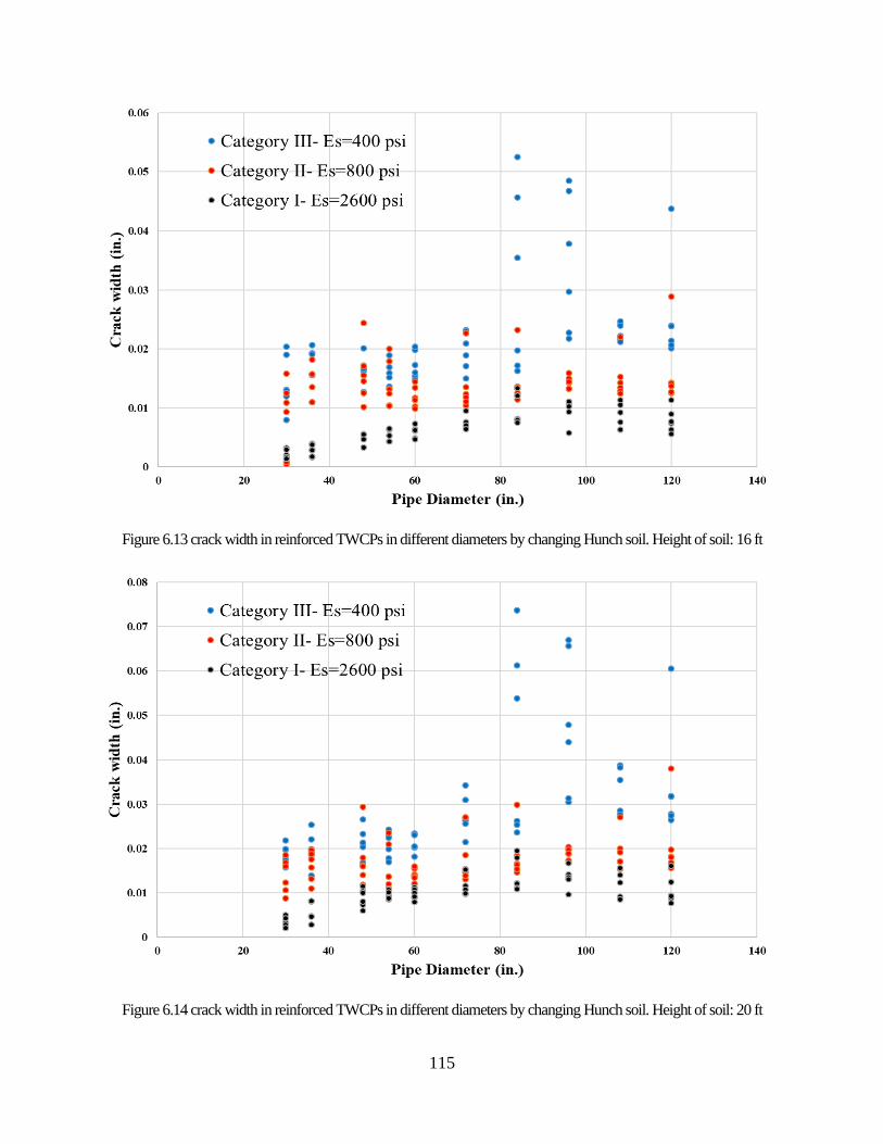
115
Figure 6.13 crack width in reinforced TWCPs in different diameters by changing Hunch soil. Height of soil: 16 ft
Figure 6.14 crack width in reinforced TWCPs in different diameters by changing Hunch soil. Height of soil: 20 ft
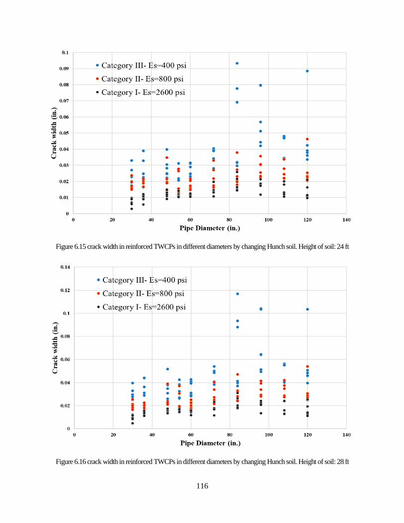
116
Figure 6.15 crack width in reinforced TWCPs in different diameters by changing Hunch soil. Height of soil: 24 ft
Figure 6.16 crack width in reinforced TWCPs in different diameters by changing Hunch soil. Height of soil: 28 ft
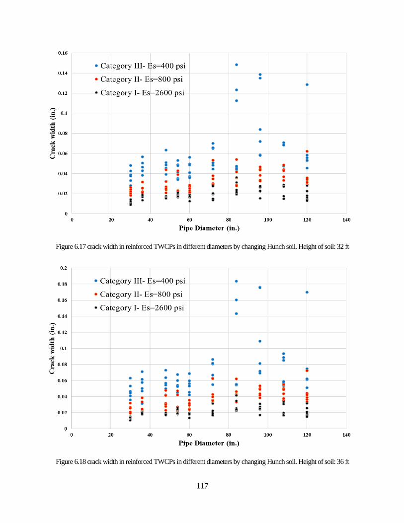
117
Figure 6.17 crack width in reinforced TWCPs in different diameters by changing Hunch soil. Height of soil: 32 ft
Figure 6.18 crack width in reinforced TWCPs in different diameters by changing Hunch soil. Height of soil: 36 ft
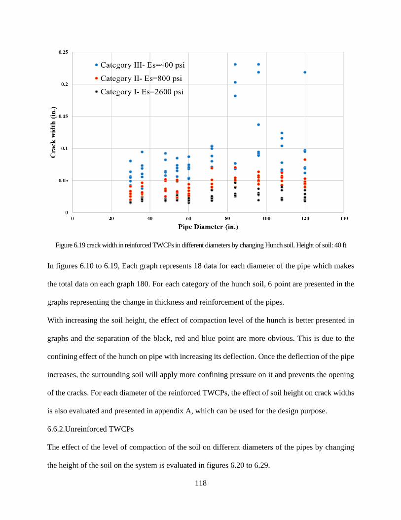
118
Figure 6.19 crack width in reinforced TWCPs in different diameters by changing Hunch soil. Height of soil: 40 ft
In figures 6.10 to 6.19, Each graph represents 18 data for each diameter of the pipe which makes
the total data on each graph 180. For each category of the hunch soil, 6 point are presented in the
graphs representing the change in thickness and reinforcement of the pipes.
With increasing the soil height, the effect of compaction level of the hunch is better presented in
graphs and the separation of the black, red and blue point are more obvious. This is due to the
confining effect of the hunch on pipe with increasing its deflection. Once the deflection of the pipe
increases, the surrounding soil will apply more confining pressure on it and prevents the opening
of the cracks. For each diameter of the reinforced TWCPs, the effect of soil height on crack widths
is also evaluated and presented in appendix A, which can be used for the design purpose.
6.6.2.Unreinforced TWCPs
The effect of the level of compaction of the soil on different diameters of the pipes by changing
the height of the soil on the system is evaluated in figures 6.20 to 6.29.
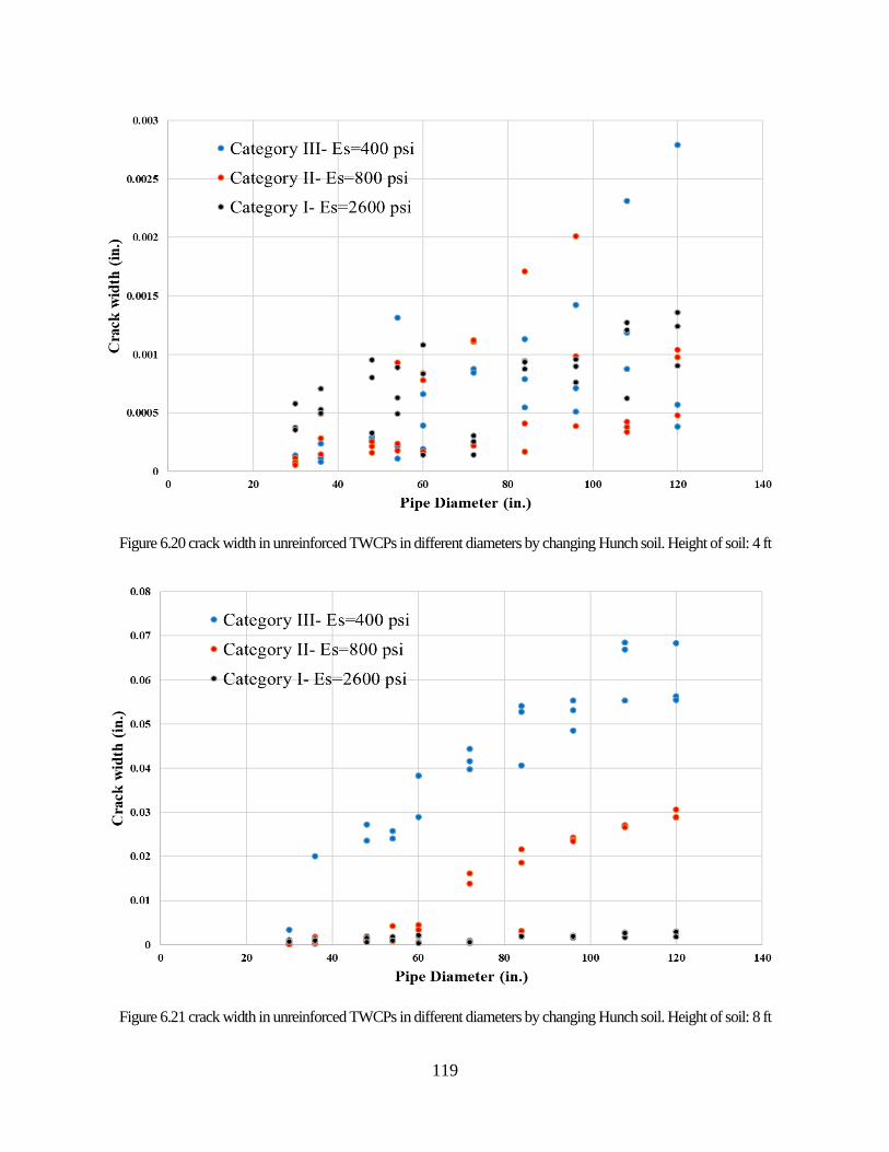
119
Figure 6.20 crack width in unreinforced TWCPs in different diameters by changing Hunch soil. Height of soil: 4 ft
Figure 6.21 crack width in unreinforced TWCPs in different diameters by changing Hunch soil. Height of soil: 8 ft
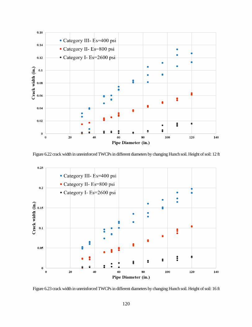
120
Figure 6.22 crack width in unreinforced TWCPs in different diameters by changing Hunch soil. Height of soil: 12 ft
Figure 6.23 crack width in unreinforced TWCPs in different diameters by changing Hunch soil. Height of soil: 16 ft
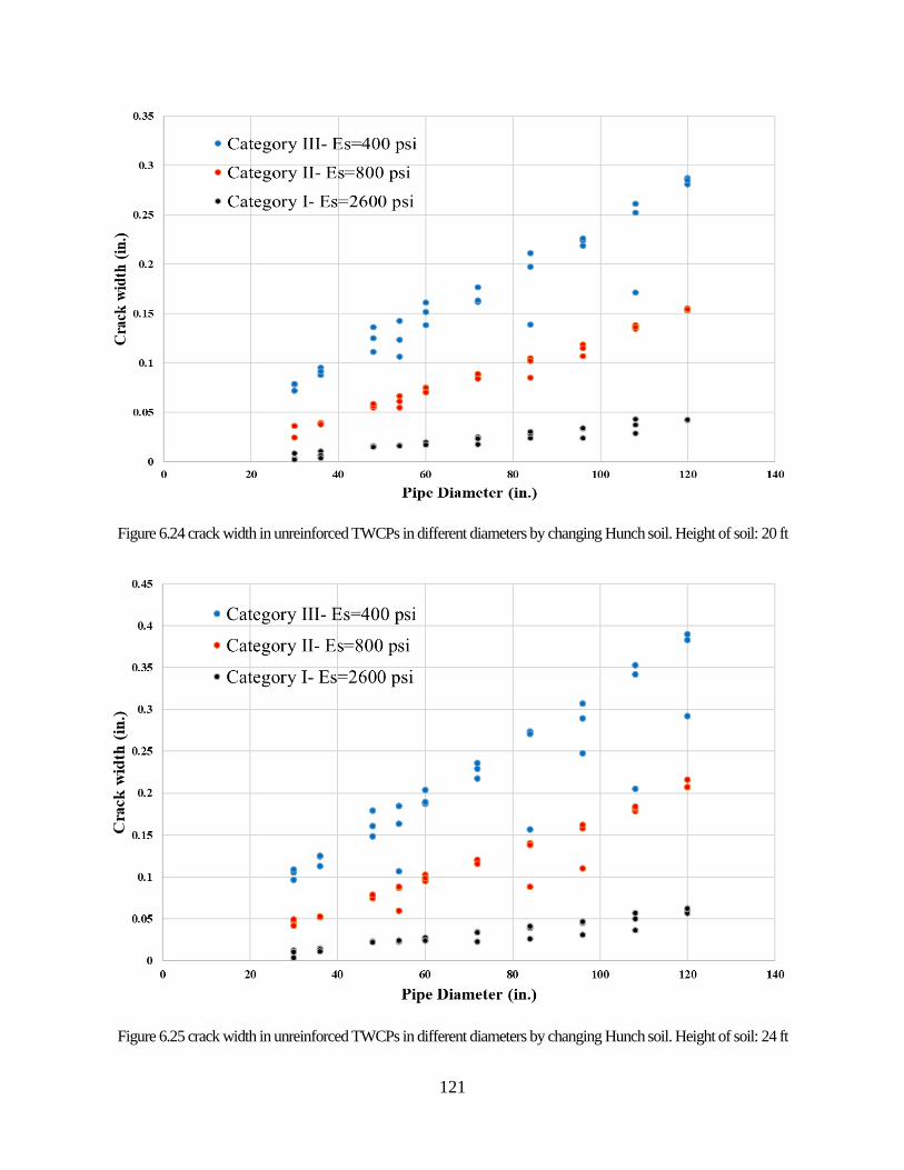
121
Figure 6.24 crack width in unreinforced TWCPs in different diameters by changing Hunch soil. Height of soil: 20 ft
Figure 6.25 crack width in unreinforced TWCPs in different diameters by changing Hunch soil. Height of soil: 24 ft
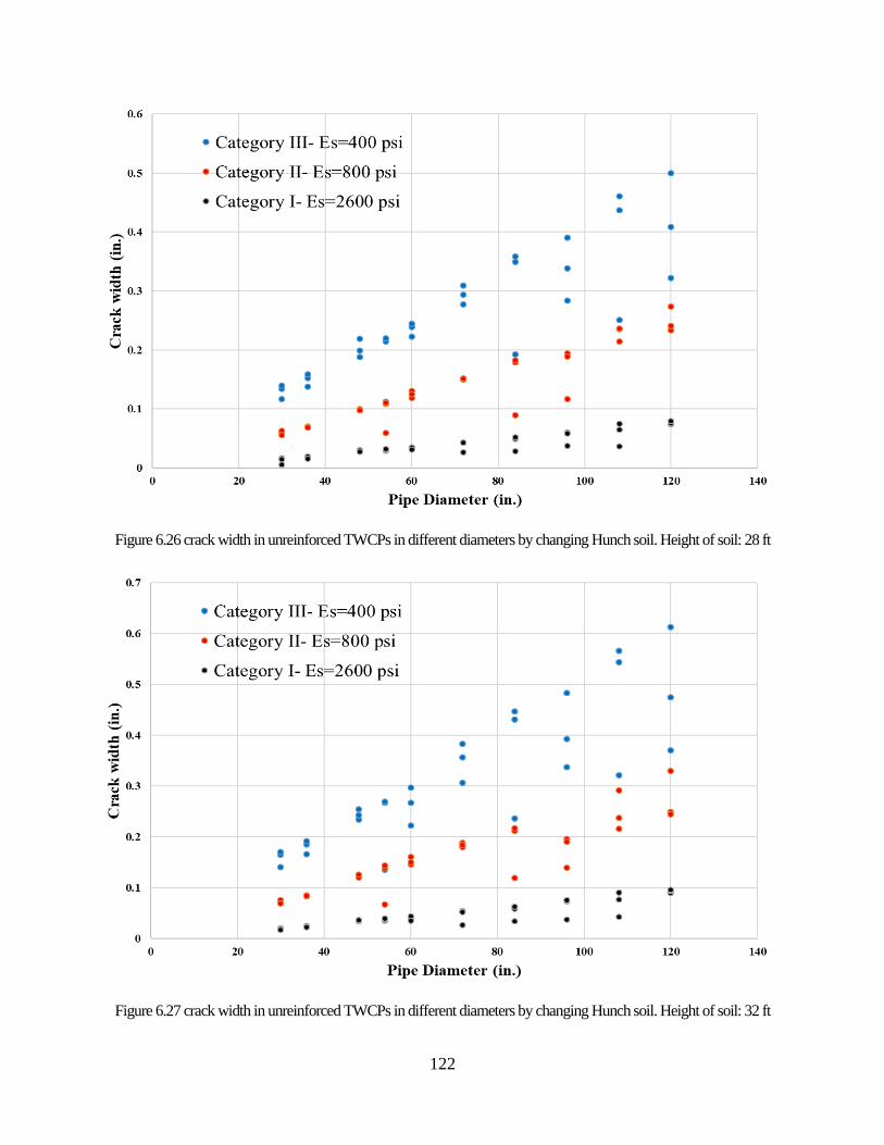
122
Figure 6.26 crack width in unreinforced TWCPs in different diameters by changing Hunch soil. Height of soil: 28 ft
Figure 6.27 crack width in unreinforced TWCPs in different diameters by changing Hunch soil. Height of soil: 32 ft
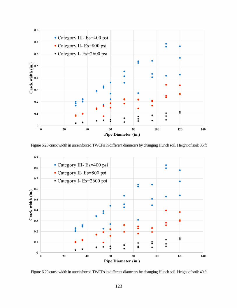
123
Figure 6.28 crack width in unreinforced TWCPs in different diameters by changing Hunch soil. Height of soil: 36 ft
Figure 6.29 crack width in unreinforced TWCPs in different diameters by changing Hunch soil. Height of soil: 40 ft
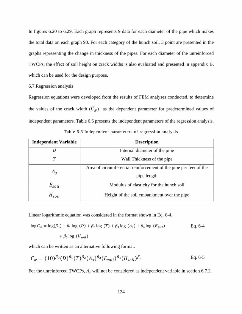
124
In figures 6.20 to 6.29, Each graph represents 9 data for each diameter of the pipe which makes
the total data on each graph 90. For each category of the hunch soil, 3 point are presented in the
graphs representing the change in thickness of the pipes. For each diameter of the unreinforced
TWCPs, the effect of soil height on crack widths is also evaluated and presented in appendix B,
which can be used for the design purpose.
6.7.Regression analysis
Regression equations were developed from the results of FEM analyses conducted, to determine
the values of the crack width (𝐶𝑤) as the dependent parameter for predetermined values of
independent parameters. Table 6.6 presents the independent parameters of the regression analysis.
Table 6.6 Independent parameters of regression analysis
Independent Variable Description
𝐷 Internal diameter of the pipe
𝑇 Wall Thickness of the pipe
𝐴𝑠 Area of circumferential reinforcement of the pipe per feet of the
pipe length
𝐸𝑠𝑜𝑖𝑙 Modulus of elasticity for the hunch soil
𝐻𝑠𝑜𝑖𝑙 Height of the soil embankment over the pipe
Linear logarithmic equation was considered in the format shown in Eq. 6-4.
log 𝐶𝑤 = log(𝛽0) + 𝛽1 log (𝐷) + 𝛽2 log (𝑇) + 𝛽3 log (𝐴𝑠) + 𝛽4 log (𝐸𝑠𝑜𝑖𝑙)
+ 𝛽5 log (𝐻𝑠𝑜𝑖𝑙)
Eq. 6-4
which can be written as an alternative following format:
𝐶𝑤 = (10)𝛽0(𝐷)𝛽1(𝑇)𝛽2(𝐴𝑠)
𝛽3(𝐸𝑠𝑜𝑖𝑙)𝛽4(𝐻𝑠𝑜𝑖𝑙)
𝛽5 Eq. 6-5
For the unreinforced TWCPs, 𝐴𝑠 will not be considered as independent variable in section 6.7.2.
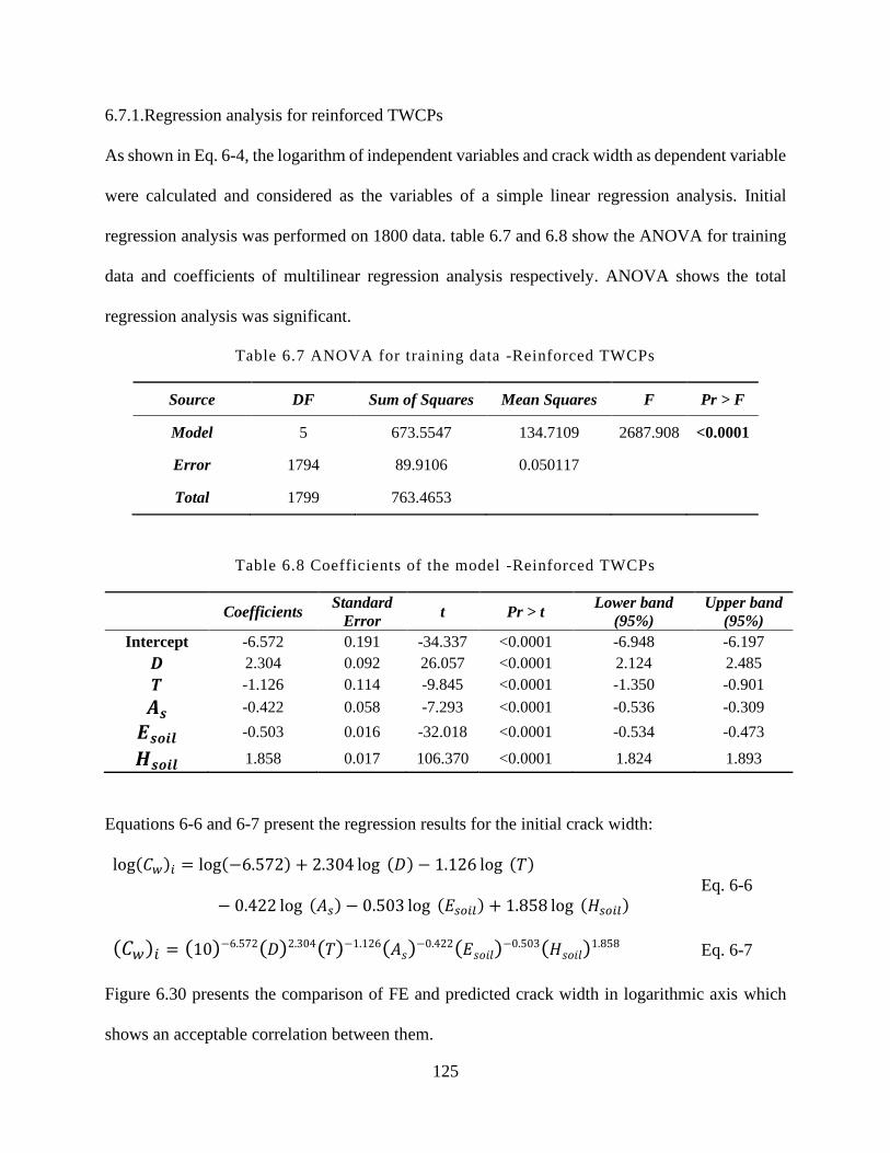
125
6.7.1.Regression analysis for reinforced TWCPs
As shown in Eq. 6-4, the logarithm of independent variables and crack width as dependent variable
were calculated and considered as the variables of a simple linear regression analysis. Initial
regression analysis was performed on 1800 data. table 6.7 and 6.8 show the ANOVA for training
data and coefficients of multilinear regression analysis respectively. ANOVA shows the total
regression analysis was significant.
Table 6.7 ANOVA for training data -Reinforced TWCPs
Source DF Sum of Squares Mean Squares F Pr > F
Model 5 673.5547 134.7109 2687.908 <0.0001
Error 1794 89.9106 0.050117
Total 1799 763.4653
Table 6.8 Coefficients of the model -Reinforced TWCPs
Coefficients Standard
Error t Pr > t
Lower band
(95%)
Upper band
(95%)
Intercept -6.572 0.191 -34.337 <0.0001 -6.948 -6.197
𝑫 2.304 0.092 26.057 <0.0001 2.124 2.485
𝑻 -1.126 0.114 -9.845 <0.0001 -1.350 -0.901
𝑨𝒔 -0.422 0.058 -7.293 <0.0001 -0.536 -0.309
𝑬𝒔𝒐𝒊𝒍 -0.503 0.016 -32.018 <0.0001 -0.534 -0.473
𝑯𝒔𝒐𝒊𝒍 1.858 0.017 106.370 <0.0001 1.824 1.893
Equations 6-6 and 6-7 present the regression results for the initial crack width:
log(𝐶𝑤)𝑖 = log(−6.572) + 2.304 log (𝐷) − 1.126 log (𝑇)
− 0.422 log (𝐴𝑠) − 0.503 log (𝐸𝑠𝑜𝑖𝑙) + 1.858 log (𝐻𝑠𝑜𝑖𝑙) Eq. 6-6
(𝐶𝑤)𝑖 = (10)−6.572(𝐷)2.304(𝑇)−1.126(𝐴𝑠)
−0.422(𝐸𝑠𝑜𝑖𝑙)−0.503(𝐻𝑠𝑜𝑖𝑙)
1.858 Eq. 6-7
Figure 6.30 presents the comparison of FE and predicted crack width in logarithmic axis which
shows an acceptable correlation between them.
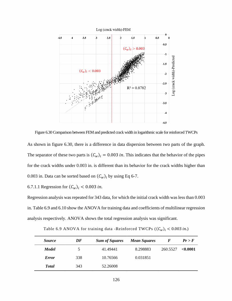
126
Figure 6.30 Comparison between FEM and predicted crack width in logarithmic scale for reinforced TWCPs
As shown in figure 6.30, there is a difference in data dispersion between two parts of the graph.
The separator of these two parts is (𝐶𝑤)𝑖 = 0.003 𝑖𝑛. This indicates that the behavior of the pipes
for the crack widths under 0.003 in. is different than its behavior for the crack widths higher than
0.003 in. Data can be sorted based on (𝐶𝑤)𝑖 by using Eq 6-7.
6.7.1.1 Regression for (𝐶𝑤)𝑖 < 0.003 𝑖𝑛.
Regression analysis was repeated for 343 data, for which the initial crack width was less than 0.003
in. Table 6.9 and 6.10 show the ANOVA for training data and coefficients of multilinear regression
analysis respectively. ANOVA shows the total regression analysis was significant.
Table 6.9 ANOVA for training data -Reinforced TWCPs ((𝐶𝑤)𝑖 < 0.003 𝑖𝑛.)
Source DF Sum of Squares Mean Squares F Pr > F
Model 5 41.49441 8.298883 260.5527 <0.0001
Error 338 10.76566 0.031851
Total 343 52.26008
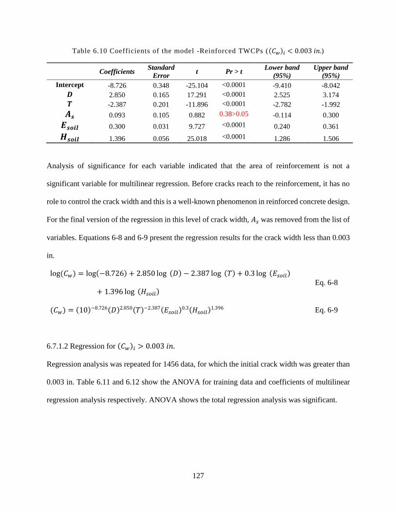
127
Table 6.10 Coefficients of the model -Reinforced TWCPs ((𝐶𝑤)𝑖 < 0.003 𝑖𝑛.)
Coefficients Standard
Error t Pr > t
Lower band
(95%)
Upper band
(95%)
Intercept -8.726 0.348 -25.104 <0.0001 -9.410 -8.042
𝑫 2.850 0.165 17.291 <0.0001 2.525 3.174
𝑻 -2.387 0.201 -11.896 <0.0001 -2.782 -1.992
𝑨𝒔 0.093 0.105 0.882 0.38>0.05 -0.114 0.300
𝑬𝒔𝒐𝒊𝒍 0.300 0.031 9.727 <0.0001 0.240 0.361
𝑯𝒔𝒐𝒊𝒍 1.396 0.056 25.018 <0.0001 1.286 1.506
Analysis of significance for each variable indicated that the area of reinforcement is not a
significant variable for multilinear regression. Before cracks reach to the reinforcement, it has no
role to control the crack width and this is a well-known phenomenon in reinforced concrete design.
For the final version of the regression in this level of crack width, 𝐴𝑠 was removed from the list of
variables. Equations 6-8 and 6-9 present the regression results for the crack width less than 0.003
in.
log(𝐶𝑤) = log(−8.726) + 2.850 log (𝐷) − 2.387 log (𝑇) + 0.3 log (𝐸𝑠𝑜𝑖𝑙)
+ 1.396 log (𝐻𝑠𝑜𝑖𝑙) Eq. 6-8
(𝐶𝑤) = (10)−8.726(𝐷)2.850(𝑇)−2.387(𝐸𝑠𝑜𝑖𝑙)
0.3(𝐻𝑠𝑜𝑖𝑙)1.396 Eq. 6-9
6.7.1.2 Regression for (𝐶𝑤)𝑖 > 0.003 𝑖𝑛.
Regression analysis was repeated for 1456 data, for which the initial crack width was greater than
0.003 in. Table 6.11 and 6.12 show the ANOVA for training data and coefficients of multilinear
regression analysis respectively. ANOVA shows the total regression analysis was significant.
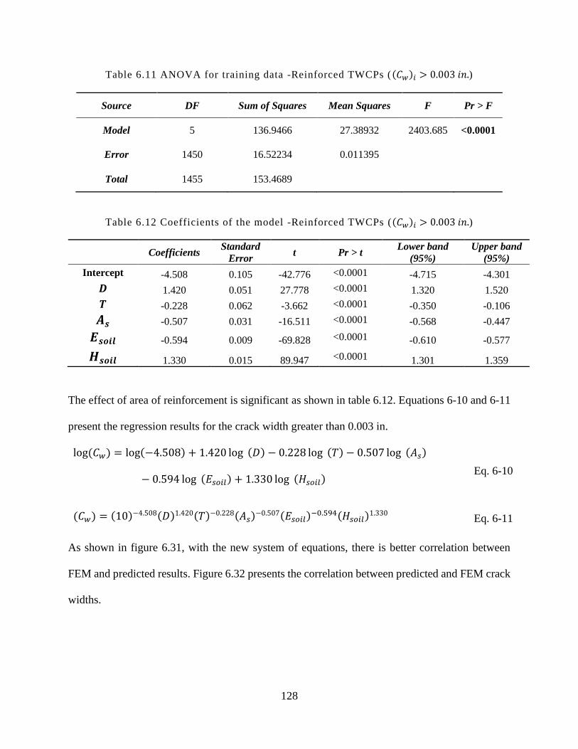
128
Table 6.11 ANOVA for training data -Reinforced TWCPs ((𝐶𝑤)𝑖 > 0.003 𝑖𝑛.)
Source DF Sum of Squares Mean Squares F Pr > F
Model 5 136.9466 27.38932 2403.685 <0.0001
Error 1450 16.52234 0.011395
Total 1455 153.4689
Table 6.12 Coefficients of the model -Reinforced TWCPs ((𝐶𝑤)𝑖 > 0.003 𝑖𝑛.)
Coefficients Standard
Error t Pr > t
Lower band
(95%)
Upper band
(95%)
Intercept -4.508 0.105 -42.776 <0.0001 -4.715 -4.301
𝑫 1.420 0.051 27.778 <0.0001 1.320 1.520
𝑻 -0.228 0.062 -3.662 <0.0001 -0.350 -0.106
𝑨𝒔 -0.507 0.031 -16.511 <0.0001 -0.568 -0.447
𝑬𝒔𝒐𝒊𝒍 -0.594 0.009 -69.828 <0.0001 -0.610 -0.577
𝑯𝒔𝒐𝒊𝒍 1.330 0.015 89.947 <0.0001 1.301 1.359
The effect of area of reinforcement is significant as shown in table 6.12. Equations 6-10 and 6-11
present the regression results for the crack width greater than 0.003 in.
log(𝐶𝑤) = log(−4.508) + 1.420 log (𝐷) − 0.228 log (𝑇) − 0.507 log (𝐴𝑠)
− 0.594 log (𝐸𝑠𝑜𝑖𝑙) + 1.330 log (𝐻𝑠𝑜𝑖𝑙) Eq. 6-10
(𝐶𝑤) = (10)−4.508(𝐷)1.420(𝑇)−0.228(𝐴𝑠)
−0.507(𝐸𝑠𝑜𝑖𝑙)−0.594(𝐻𝑠𝑜𝑖𝑙)
1.330 Eq. 6-11
As shown in figure 6.31, with the new system of equations, there is better correlation between
FEM and predicted results. Figure 6.32 presents the correlation between predicted and FEM crack
widths.
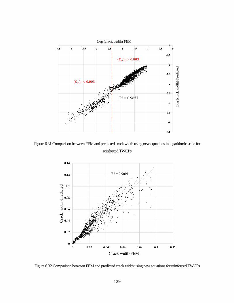
129
Figure 6.31 Comparison between FEM and predicted crack width using new equations in logarithmic scale for
reinforced TWCPs
Figure 6.32 Comparison between FEM and predicted crack width using new equations for reinforced TWCPs
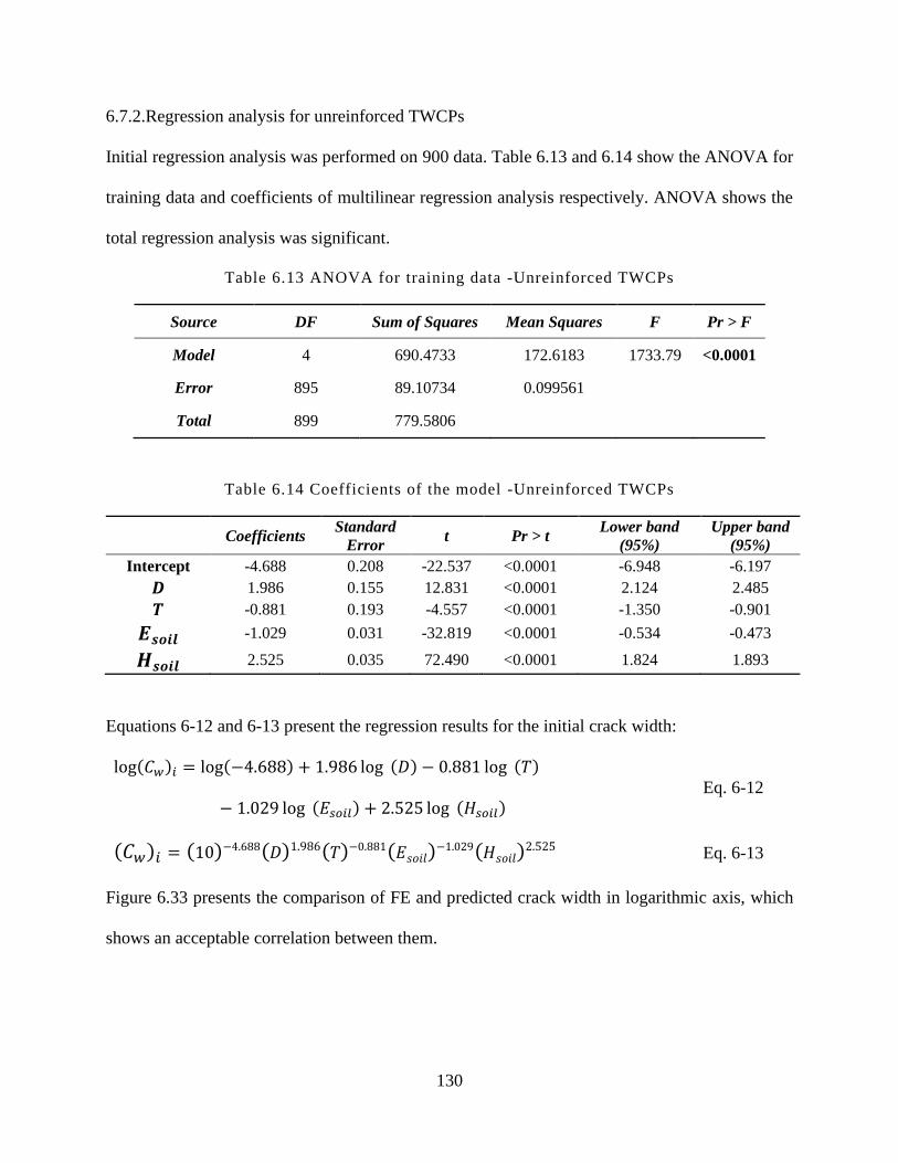
130
6.7.2.Regression analysis for unreinforced TWCPs
Initial regression analysis was performed on 900 data. Table 6.13 and 6.14 show the ANOVA for
training data and coefficients of multilinear regression analysis respectively. ANOVA shows the
total regression analysis was significant.
Table 6.13 ANOVA for training data -Unreinforced TWCPs
Source DF Sum of Squares Mean Squares F Pr > F
Model 4 690.4733 172.6183 1733.79 <0.0001
Error 895 89.10734 0.099561
Total 899 779.5806
Table 6.14 Coefficients of the model -Unreinforced TWCPs
Coefficients Standard
Error t Pr > t
Lower band
(95%)
Upper band
(95%)
Intercept -4.688 0.208 -22.537 <0.0001 -6.948 -6.197
𝑫 1.986 0.155 12.831 <0.0001 2.124 2.485
𝑻 -0.881 0.193 -4.557 <0.0001 -1.350 -0.901
𝑬𝒔𝒐𝒊𝒍 -1.029 0.031 -32.819 <0.0001 -0.534 -0.473
𝑯𝒔𝒐𝒊𝒍 2.525 0.035 72.490 <0.0001 1.824 1.893
Equations 6-12 and 6-13 present the regression results for the initial crack width:
log(𝐶𝑤)𝑖 = log(−4.688) + 1.986 log (𝐷) − 0.881 log (𝑇)
− 1.029 log (𝐸𝑠𝑜𝑖𝑙) + 2.525 log (𝐻𝑠𝑜𝑖𝑙) Eq. 6-12
(𝐶𝑤)𝑖 = (10)−4.688(𝐷)1.986(𝑇)−0.881(𝐸𝑠𝑜𝑖𝑙)
−1.029(𝐻𝑠𝑜𝑖𝑙)2.525 Eq. 6-13
Figure 6.33 presents the comparison of FE and predicted crack width in logarithmic axis, which
shows an acceptable correlation between them.
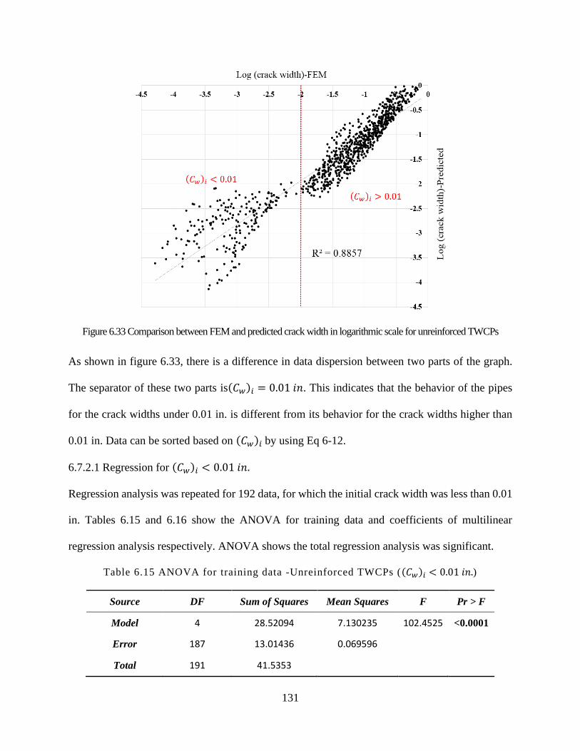
131
Figure 6.33 Comparison between FEM and predicted crack width in logarithmic scale for unreinforced TWCPs
As shown in figure 6.33, there is a difference in data dispersion between two parts of the graph.
The separator of these two parts is(𝐶𝑤)𝑖 = 0.01 𝑖𝑛. This indicates that the behavior of the pipes
for the crack widths under 0.01 in. is different from its behavior for the crack widths higher than
0.01 in. Data can be sorted based on (𝐶𝑤)𝑖 by using Eq 6-12.
6.7.2.1 Regression for (𝐶𝑤)𝑖 < 0.01 𝑖𝑛.
Regression analysis was repeated for 192 data, for which the initial crack width was less than 0.01
in. Tables 6.15 and 6.16 show the ANOVA for training data and coefficients of multilinear
regression analysis respectively. ANOVA shows the total regression analysis was significant.
Table 6.15 ANOVA for training data -Unreinforced TWCPs ((𝐶𝑤)𝑖 < 0.01 𝑖𝑛.)
Source DF Sum of Squares Mean Squares F Pr > F
Model 4 28.52094 7.130235 102.4525 <0.0001
Error 187 13.01436 0.069596
Total 191 41.5353
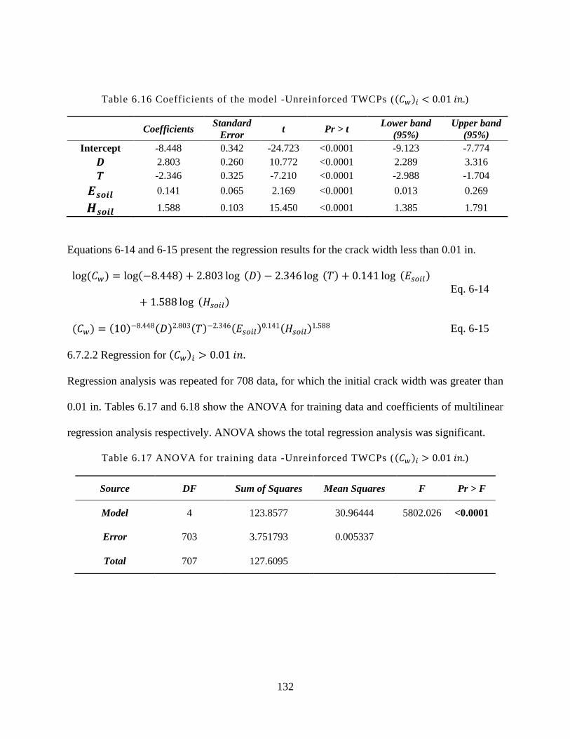
132
Table 6.16 Coefficients of the model -Unreinforced TWCPs ((𝐶𝑤)𝑖 < 0.01 𝑖𝑛.)
Coefficients Standard
Error t Pr > t
Lower band
(95%)
Upper band
(95%)
Intercept -8.448 0.342 -24.723 <0.0001 -9.123 -7.774
𝑫 2.803 0.260 10.772 <0.0001 2.289 3.316
𝑻 -2.346 0.325 -7.210 <0.0001 -2.988 -1.704
𝑬𝒔𝒐𝒊𝒍 0.141 0.065 2.169 <0.0001 0.013 0.269
𝑯𝒔𝒐𝒊𝒍 1.588 0.103 15.450 <0.0001 1.385 1.791
Equations 6-14 and 6-15 present the regression results for the crack width less than 0.01 in.
log(𝐶𝑤) = log(−8.448) + 2.803 log (𝐷) − 2.346 log (𝑇) + 0.141 log (𝐸𝑠𝑜𝑖𝑙)
+ 1.588 log (𝐻𝑠𝑜𝑖𝑙) Eq. 6-14
(𝐶𝑤) = (10)−8.448(𝐷)2.803(𝑇)−2.346(𝐸𝑠𝑜𝑖𝑙)
0.141(𝐻𝑠𝑜𝑖𝑙)1.588 Eq. 6-15
6.7.2.2 Regression for (𝐶𝑤)𝑖 > 0.01 𝑖𝑛.
Regression analysis was repeated for 708 data, for which the initial crack width was greater than
0.01 in. Tables 6.17 and 6.18 show the ANOVA for training data and coefficients of multilinear
regression analysis respectively. ANOVA shows the total regression analysis was significant.
Table 6.17 ANOVA for training data -Unreinforced TWCPs ((𝐶𝑤)𝑖 > 0.01 𝑖𝑛.)
Source DF Sum of Squares Mean Squares F Pr > F
Model 4 123.8577 30.96444 5802.026 <0.0001
Error 703 3.751793 0.005337
Total 707 127.6095
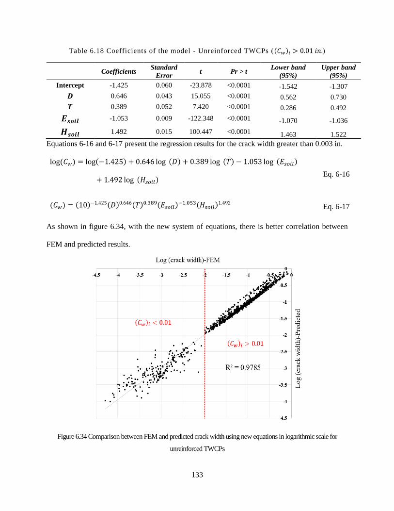
133
Table 6.18 Coefficients of the model - Unreinforced TWCPs ((𝐶𝑤)𝑖 > 0.01 𝑖𝑛.)
Coefficients Standard
Error t Pr > t
Lower band
(95%)
Upper band
(95%)
Intercept -1.425 0.060 -23.878 <0.0001 -1.542 -1.307
𝑫 0.646 0.043 15.055 <0.0001 0.562 0.730
𝑻 0.389 0.052 7.420 <0.0001 0.286 0.492
𝑬𝒔𝒐𝒊𝒍 -1.053 0.009 -122.348 <0.0001 -1.070 -1.036
𝑯𝒔𝒐𝒊𝒍 1.492 0.015 100.447 <0.0001 1.463 1.522
Equations 6-16 and 6-17 present the regression results for the crack width greater than 0.003 in.
log(𝐶𝑤) = log(−1.425) + 0.646 log (𝐷) + 0.389 log (𝑇) − 1.053 log (𝐸𝑠𝑜𝑖𝑙)
+ 1.492 log (𝐻𝑠𝑜𝑖𝑙) Eq. 6-16
(𝐶𝑤) = (10)−1.425(𝐷)0.646(𝑇)0.389(𝐸𝑠𝑜𝑖𝑙)
−1.053(𝐻𝑠𝑜𝑖𝑙)1.492 Eq. 6-17
As shown in figure 6.34, with the new system of equations, there is better correlation between
FEM and predicted results.
Figure 6.34 Comparison between FEM and predicted crack width using new equations in logarithmic scale for
unreinforced TWCPs
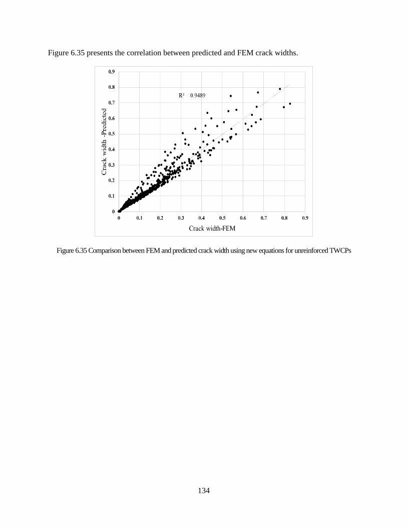
134
Figure 6.35 presents the correlation between predicted and FEM crack widths.
Figure 6.35 Comparison between FEM and predicted crack width using new equations for unreinforced TWCPs
135
CHAPTER 7. SUMMARY AND CONCLUSIONS
7.1.Summary
Buried pipe systems have been designed based on two general methods considering the soil-pipe
structural interaction: that is, evaluating the pipe as a rigid pipe, or evaluating it as a flexible pipe.
Rigid and flexible pipes are distinguished by the deflection ratio or by the relative stiffness of the
pipe. Rigid pipe systems only rely on the active soil pressure, and primarily resist the loads on the
pipe by carrying moment and shear in the pipe wall and start showing signs of structural failure
before being vertically deflected up to 2 % of their inside diameter. Flexible pipe systems carry
load by deflecting out into the soil to pick up additional passive soil pressure, which then results
primarily in compressive forces in the pipe wall.
Flexible pipes, made from metal and plastic, have lower material price compare to rigid ones but
the installation of these pipes needs more soil compaction effort and thus results in higher
construction price. With restricted specifications of design and installation of flexible pipes,
engineers and contractors need to accept the installation risks, which come with them. Concrete
pipe represents the predominant pipe material used for rigid pipe systems in the storm sewer
market in the US. Concrete pipe is very durable and utilizes design methods that have been in
place for decades to design a pipe product, which ensures that concrete pipe can take a large portion
of the soil backfill load on its own. This enables the pipe to be independent from the reaction of
the surrounding soil and thus reduces the compaction efforts during the construction process.
The main goal of this research was to evaluate the concept of thin-walled concrete pipe (TWCP)
as a Semi-Rigid Pipe. The idea was to reduce the thickness and reinforcement of the current
reinforced concrete pipes to increase their deflection before failure and control the crack formation
and width by using synthetic fibers. The flexibility of these pipes will enable them to use the
136
passive pressure of surrounding soil and in turn, relieves the pipe of the burden of carrying the soil
load through moment and shear in the pipe wall (as standard reinforced concrete pipe does) and
allows it to perform primarily under compressive stress in the pipe wall. In addition, the risk of
uncompact soil during installation process will be minimized in these pipes having a minimum
required self-rigidity. This This type of concrete pipe would be lighter, cheaper, and more durable
than what is currently in use while still providing a pipe product much less dependent upon
installation conditions than the very flexible metal and plastic pipes in the American market.
The following steps were taken to investigate the concept of TWCPs:
• Comprehensive experimental investigations were conducted in two phases:
o The first phase was to understand the behavior of synthetic fiber reinforced TWCPs in
Industrial scale pipe production using a common industrial concrete mix design. In this
phase, 44 pipes were created and TEB test was performed on all the pipes. The load-
deformation curve for all tested specimens was extracted and the cracking behavior of
the pipes with and without using synthetic fibers was observed.
o The second phase was to perform experimental study on crack development in
synthetic fiber reinforced concrete specimens. In this phase, 12 beam specimens were
created using ASTM 1609 recommendations. The beams were tested in two groups of
six beams under three and four- point bending test setup. Crack width was measured
using two-dimensional digital image correlation (DIC) method.
• Finite element modeling was performed in three phases:
o The first phase of FE modeling was to mimic the behavior of bending test specimens
to find a method with which the crack widths can be measured using a FE approach. In
this phase three-dimensional FE models has been created to simulate the three-point

137
and four-point bending tests. By using a three-phase uniaxial tensile curve for Syn-
FRC, the load-deflection curves of the tests specimens were obtained and matched with
the tests results. A crack width measurement method with FE was proposed
o The second phase of FE modeling was to create models to mimic the behavior of
TWCPs under TEB test. This phase helped to find the bests tensile stress softening
curve for the Syn-FRC, used in industry. The TWCPs in industrial level are created
using a dry mixed concrete using a packer head equipment. The effect of industrial
process on the material property of the Syn-FRC was evaluated in this phase as well as
the capability of FE modeling to mimic the TEB tests.
o Since interaction of pipe with the soil has a great impact on structural behavior of
TWCP systems in third phase of FE modeling, a soil-pipe interaction was developed to
simulate the behavior of TWCPs under step by step increasing loads of the soil backfill.
A model change method was utilized to mimic staged loading of the backfill on the
soil-pipe system. The FE crack width measurement, already proved to be reliable in
first phase of FE modeling, was used to measure the crack width in TWCPs inside the
soil.
• Parametric study was conducted on soil-pipe interaction FE models. 180 models with
reinforced and 90 models with unreinforced TWCPs were created and during ten steps of
loading (each of which with four feet soil of backfill) the crack width calculated. The results
were presented in different design graphs.
• Multi variate regression analysis was performed on two sets of data for reinforced and
unreinforced TWCPs and the results were presented in form of crack width equations.
138
7.2.Conclusion remarks
• Following remarks can be concluded from TEB tests performed on TWCPs:
o Discrete synthetic fibers increased the shear capacity of concrete, delayed shear
failure mode, and significantly enhanced the capacity of pipe to carry the loads with
the use of reduced steel reinforcement.
o The reductions in pipe thickness in the experiments were in the ranges of 35% and
50% for small and large diameter concrete pipe, respectively. This reduction
increased the flexibility of the pipes to reach 3% of deflection before its ultimate
load. This will let the pipe deform toward the surrounding soil to utilize the passive
soil pressure.
o To have a guideline it was set for TW pipes to have a minimum stiffness of 690
kPa (100 psi) at 3 % deflection. Among thirty-four tested TW pipes with synthetic
fibers, thirty-two TW pipes (97 %) satisfied the suggested minimum pipe stiffness
(100 psi) at 3% deflection.
• DIC method was successfully adopted and calibrated to measure the crack width and has been
proven to be a reliable method to do this. By using 1% volume fraction of synthetic fibers, it
has been shown that the behavior of bending specimens will be drastically change and the
bridging effect will act to overcome the increasing of crack width.
• The three-phase uniaxial tensile model was used successfully to mimic the behavior of bending
specimens and TEB test of the TWCPs. The crack patterns observed in TEB tests could be
detected in FE models. Comparison between the experimental crack measurement data with
those measured by FE proved the method to be reliable.
139
• From parametric study on the crack width of TWCPs in soil-pipe interaction models, design
graphs were produced. Following remarks are the most important conclusions form the graphs:
o The effect of level of compaction for hunch is not significant if the depth of backfill
is up to 4 ft for both reinforced and unreinforced TWCPs
o It is possible to design all diameters of reinforced TWCPs to withstand 8 ft of soil
pressure with a crack with less than 0.01 in. by using all categories of soil for hunch.
o It is possible to design all diameters of reinforced TWCPs to withstand 12 ft of soil
pressure with a crack with less than 0.01 in. using soils in category I and II for
hunch.
o Using soils in category I for hunch, it is possible to design all diameters of
reinforced TWCPs to withstand up to 24 ft of soil pressure with a crack with less
than 0.01 in.
o It is possible to design all diameters of unreinforced TWCPs to withstand 8 ft of
soil pressure with a crack with less than 0.01 in. by using soils in category I for
hunch.
• Multi variate regression analysis showed that there is a boundary at crack width of 0.003 in.
and 0.01 in. for reinforced and unreinforced TWCPs respectively. To calculate crack width
above and below this boundary different equations should be used.
7.3.Suggested future studies
TWCPs are the new category of concrete pipes and this research began to investigate the possibility
of production and structural concepts of these pipes on which more investigations needed. Some
suggestions for future studies of this research are:

140
• The effect of using the soils with different parameters in backfill and bedding should be
studied by creating more FE models
• Trench installation should be investigated to see the effect of native soil and trench with
on the behavior of the pipes.
• Long term deflection should be considered to investigate the effect of time on crack width.
• The effect of traffic loads on the cracks of TWCPs buried under less than 4 ft of soil should
be investigated.
141
APPENDIX A. GRAPHS OF CRACK WIDTH FOR REINFORCED TWCPs
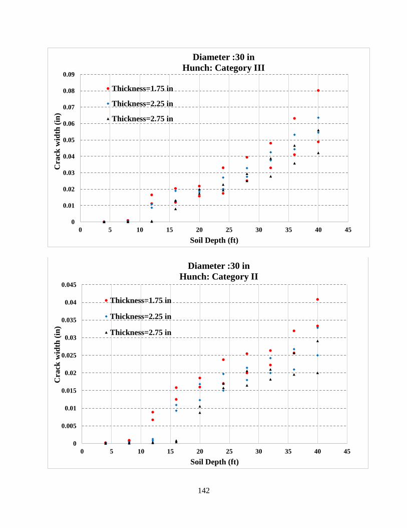
142
0
0.01
0.02
0.03
0.04
0.05
0.06
0.07
0.08
0.09
0 5 10 15 20 25 30 35 40 45
Cra
ck w
idth
(in
)
Soil Depth (ft)
Diameter :30 in
Hunch: Category III
Thickness=1.75 in
Thickness=2.25 in
Thickness=2.75 in
0
0.005
0.01
0.015
0.02
0.025
0.03
0.035
0.04
0.045
0 5 10 15 20 25 30 35 40 45
Cra
ck w
idth
(in
)
Soil Depth (ft)
Diameter :30 in
Hunch: Category II
Thickness=1.75 in
Thickness=2.25 in
Thickness=2.75 in

143
0
0.002
0.004
0.006
0.008
0.01
0.012
0.014
0.016
0.018
0 5 10 15 20 25 30 35 40 45
Cra
ck w
idth
(in
)
Soil Depth (ft)
Diameter :30 in
Hunch: Category I
Thickness=1.75 in
Thickness=2.25 in
Thickness=2.75 in
0
0.01
0.02
0.03
0.04
0.05
0.06
0.07
0.08
0.09
0.1
0 5 10 15 20 25 30 35 40 45
Cra
ck w
idth
(in
)
Soil Depth (ft)
Diameter :36 in
Hunch: Category III
Thickness=2.0 in
Thickness=2.5 in
Thickness=3.0 in
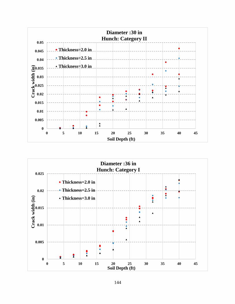
144
0
0.005
0.01
0.015
0.02
0.025
0.03
0.035
0.04
0.045
0.05
0 5 10 15 20 25 30 35 40 45
Cra
ck w
idth
(in
)
Soil Depth (ft)
Diameter :30 in
Hunch: Category II
Thickness=2.0 in
Thickness=2.5 in
Thickness=3.0 in
0
0.005
0.01
0.015
0.02
0.025
0 5 10 15 20 25 30 35 40 45
Cra
ck w
idth
(in
)
Soil Depth (ft)
Diameter :36 in
Hunch: Category I
Thickness=2.0 in
Thickness=2.5 in
Thickness=3.0 in
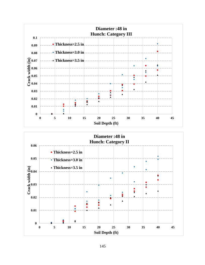
145
0
0.01
0.02
0.03
0.04
0.05
0.06
0.07
0.08
0.09
0.1
0 5 10 15 20 25 30 35 40 45
Cra
ck w
idth
(in
)
Soil Depth (ft)
Diameter :48 in
Hunch: Category III
Thickness=2.5 in
Thickness=3.0 in
Thickness=3.5 in
0
0.01
0.02
0.03
0.04
0.05
0.06
0 5 10 15 20 25 30 35 40 45
Cra
ck w
idth
(in
)
Soil Depth (ft)
Diameter :48 in
Hunch: Category II
Thickness=2.5 in
Thickness=3.0 in
Thickness=3.5 in
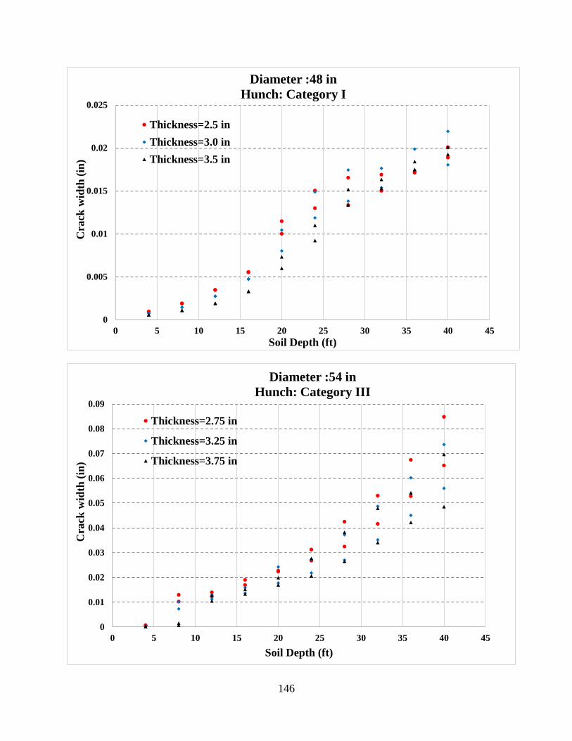
146
0
0.005
0.01
0.015
0.02
0.025
0 5 10 15 20 25 30 35 40 45
Cra
ck w
idth
(in
)
Soil Depth (ft)
Diameter :48 in
Hunch: Category I
Thickness=2.5 in
Thickness=3.0 in
Thickness=3.5 in
0
0.01
0.02
0.03
0.04
0.05
0.06
0.07
0.08
0.09
0 5 10 15 20 25 30 35 40 45
Cra
ck w
idth
(in
)
Soil Depth (ft)
Diameter :54 in
Hunch: Category III
Thickness=2.75 in
Thickness=3.25 in
Thickness=3.75 in
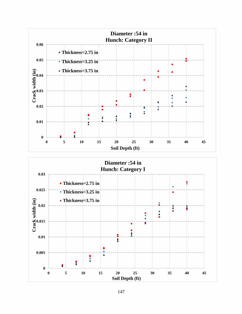
147
0
0.01
0.02
0.03
0.04
0.05
0.06
0 5 10 15 20 25 30 35 40 45
Cra
ck w
idth
(in
)
Soil Depth (ft)
Diameter :54 in
Hunch: Category II
Thickness=2.75 in
Thickness=3.25 in
Thickness=3.75 in
0
0.005
0.01
0.015
0.02
0.025
0.03
0 5 10 15 20 25 30 35 40 45
Cra
ck w
idth
(in
)
Soil Depth (ft)
Diameter :54 in
Hunch: Category I
Thickness=2.75 in
Thickness=3.25 in
Thickness=3.75 in
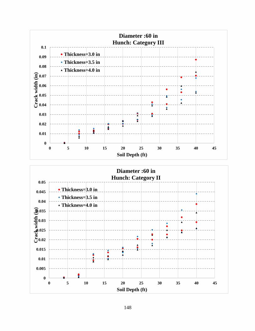
148
0
0.01
0.02
0.03
0.04
0.05
0.06
0.07
0.08
0.09
0.1
0 5 10 15 20 25 30 35 40 45
Cra
ck w
idth
(in
)
Soil Depth (ft)
Diameter :60 in
Hunch: Category III
Thickness=3.0 in
Thickness=3.5 in
Thickness=4.0 in
0
0.005
0.01
0.015
0.02
0.025
0.03
0.035
0.04
0.045
0.05
0 5 10 15 20 25 30 35 40 45
Cra
ck w
idth
(in
)
Soil Depth (ft)
Diameter :60 in
Hunch: Category II
Thickness=3.0 in
Thickness=3.5 in
Thickness=4.0 in
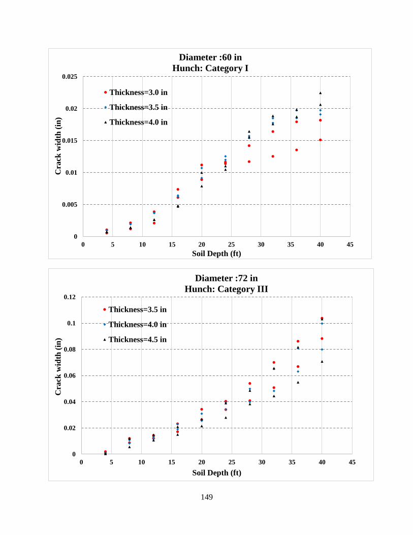
149
0
0.005
0.01
0.015
0.02
0.025
0 5 10 15 20 25 30 35 40 45
Cra
ck w
idth
(in
)
Soil Depth (ft)
Diameter :60 in
Hunch: Category I
Thickness=3.0 in
Thickness=3.5 in
Thickness=4.0 in
0
0.02
0.04
0.06
0.08
0.1
0.12
0 5 10 15 20 25 30 35 40 45
Cra
ck w
idth
(in
)
Soil Depth (ft)
Diameter :72 in
Hunch: Category III
Thickness=3.5 in
Thickness=4.0 in
Thickness=4.5 in
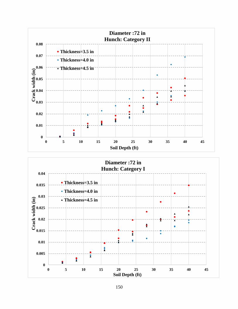
150
0
0.01
0.02
0.03
0.04
0.05
0.06
0.07
0.08
0 5 10 15 20 25 30 35 40 45
Cra
ck w
idth
(in
)
Soil Depth (ft)
Diameter :72 in
Hunch: Category II
Thickness=3.5 in
Thickness=4.0 in
Thickness=4.5 in
0
0.005
0.01
0.015
0.02
0.025
0.03
0.035
0.04
0 5 10 15 20 25 30 35 40 45
Cra
ck w
idth
(in
)
Soil Depth (ft)
Diameter :72 in
Hunch: Category I
Thickness=3.5 in
Thickness=4.0 in
Thickness=4.5 in
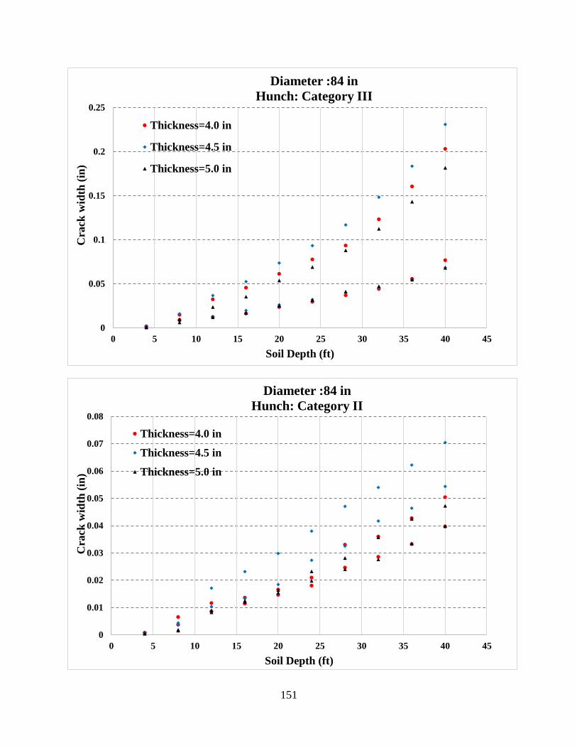
151
0
0.05
0.1
0.15
0.2
0.25
0 5 10 15 20 25 30 35 40 45
Cra
ck w
idth
(in
)
Soil Depth (ft)
Diameter :84 in
Hunch: Category III
Thickness=4.0 in
Thickness=4.5 in
Thickness=5.0 in
0
0.01
0.02
0.03
0.04
0.05
0.06
0.07
0.08
0 5 10 15 20 25 30 35 40 45
Cra
ck w
idth
(in
)
Soil Depth (ft)
Diameter :84 in
Hunch: Category II
Thickness=4.0 in
Thickness=4.5 in
Thickness=5.0 in
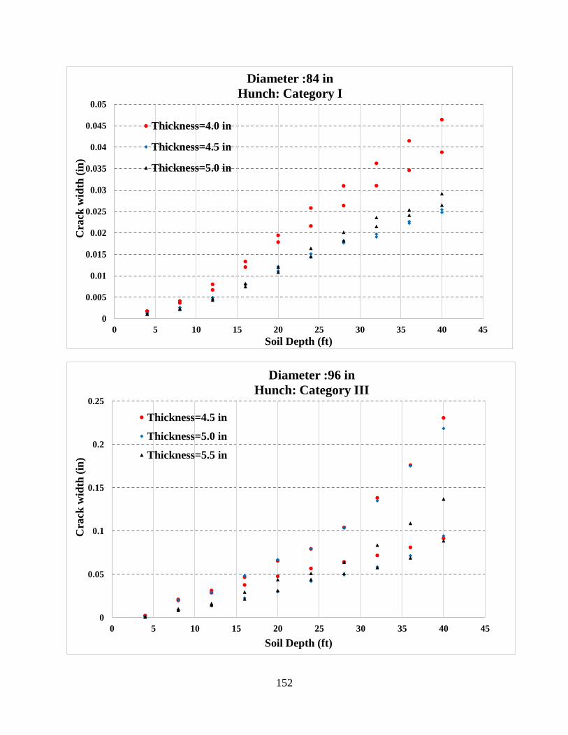
152
0
0.005
0.01
0.015
0.02
0.025
0.03
0.035
0.04
0.045
0.05
0 5 10 15 20 25 30 35 40 45
Cra
ck w
idth
(in
)
Soil Depth (ft)
Diameter :84 in
Hunch: Category I
Thickness=4.0 in
Thickness=4.5 in
Thickness=5.0 in
0
0.05
0.1
0.15
0.2
0.25
0 5 10 15 20 25 30 35 40 45
Cra
ck w
idth
(in
)
Soil Depth (ft)
Diameter :96 in
Hunch: Category III
Thickness=4.5 in
Thickness=5.0 in
Thickness=5.5 in
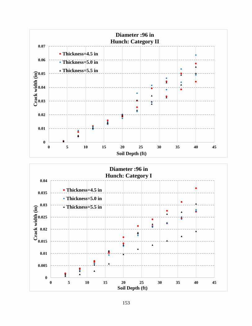
153
0
0.01
0.02
0.03
0.04
0.05
0.06
0.07
0 5 10 15 20 25 30 35 40 45
Cra
ck w
idth
(in
)
Soil Depth (ft)
Diameter :96 in
Hunch: Category II
Thickness=4.5 in
Thickness=5.0 in
Thickness=5.5 in
0
0.005
0.01
0.015
0.02
0.025
0.03
0.035
0.04
0 5 10 15 20 25 30 35 40 45
Cra
ck w
idth
(in
)
Soil Depth (ft)
Diameter :96 in
Hunch: Category I
Thickness=4.5 in
Thickness=5.0 in
Thickness=5.5 in
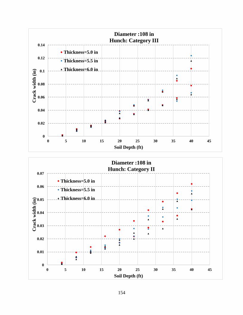
154
0
0.02
0.04
0.06
0.08
0.1
0.12
0.14
0 5 10 15 20 25 30 35 40 45
Cra
ck w
idth
(in
)
Soil Depth (ft)
Diameter :108 in
Hunch: Category III
Thickness=5.0 in
Thickness=5.5 in
Thickness=6.0 in
0
0.01
0.02
0.03
0.04
0.05
0.06
0.07
0 5 10 15 20 25 30 35 40 45
Cra
ck w
idth
(in
)
Soil Depth (ft)
Diameter :108 in
Hunch: Category II
Thickness=5.0 in
Thickness=5.5 in
Thickness=6.0 in
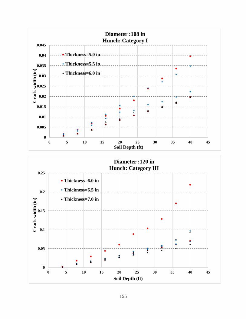
155
0
0.005
0.01
0.015
0.02
0.025
0.03
0.035
0.04
0.045
0 5 10 15 20 25 30 35 40 45
Cra
ck w
idth
(in
)
Soil Depth (ft)
Diameter :108 in
Hunch: Category I
Thickness=5.0 in
Thickness=5.5 in
Thickness=6.0 in
0
0.05
0.1
0.15
0.2
0.25
0 5 10 15 20 25 30 35 40 45
Cra
ck w
idth
(in
)
Soil Depth (ft)
Diameter :120 in
Hunch: Category III
Thickness=6.0 in
Thickness=6.5 in
Thickness=7.0 in
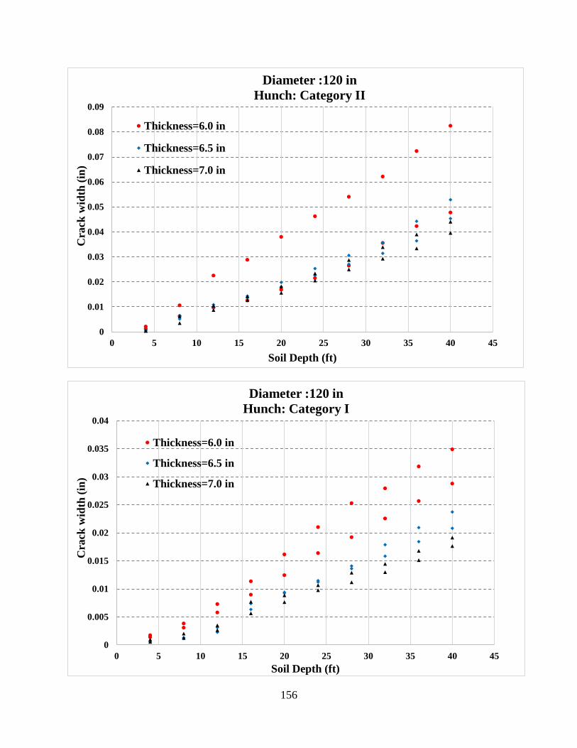
156
0
0.01
0.02
0.03
0.04
0.05
0.06
0.07
0.08
0.09
0 5 10 15 20 25 30 35 40 45
Cra
ck w
idth
(in
)
Soil Depth (ft)
Diameter :120 in
Hunch: Category II
Thickness=6.0 in
Thickness=6.5 in
Thickness=7.0 in
0
0.005
0.01
0.015
0.02
0.025
0.03
0.035
0.04
0 5 10 15 20 25 30 35 40 45
Cra
ck w
idth
(in
)
Soil Depth (ft)
Diameter :120 in
Hunch: Category I
Thickness=6.0 in
Thickness=6.5 in
Thickness=7.0 in

157
APPENDIX B. GRAPHS OF CRACK WIDTH FOR UNREINFORCED TWCPs
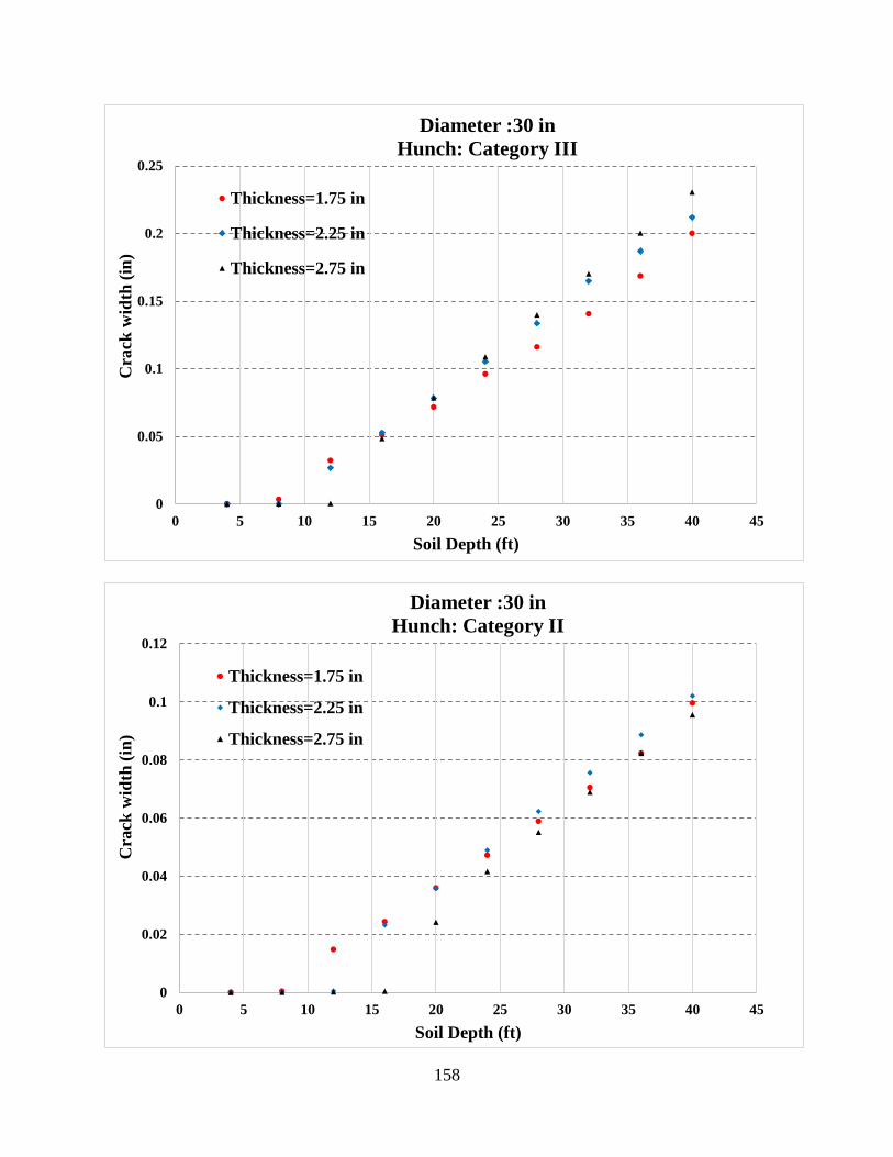
158
0
0.05
0.1
0.15
0.2
0.25
0 5 10 15 20 25 30 35 40 45
Cra
ck w
idth
(in
)
Soil Depth (ft)
Diameter :30 in
Hunch: Category III
Thickness=1.75 in
Thickness=2.25 in
Thickness=2.75 in
0
0.02
0.04
0.06
0.08
0.1
0.12
0 5 10 15 20 25 30 35 40 45
Cra
ck w
idth
(in
)
Soil Depth (ft)
Diameter :30 in
Hunch: Category II
Thickness=1.75 in
Thickness=2.25 in
Thickness=2.75 in
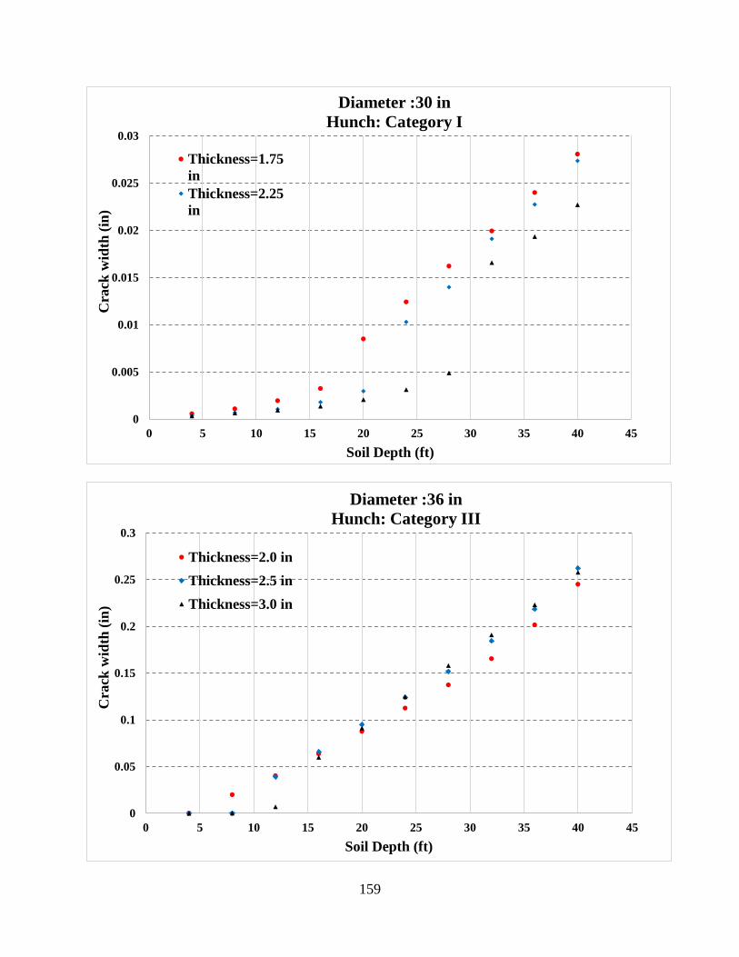
159
0
0.005
0.01
0.015
0.02
0.025
0.03
0 5 10 15 20 25 30 35 40 45
Cra
ck w
idth
(in
)
Soil Depth (ft)
Diameter :30 in
Hunch: Category I
Thickness=1.75
in
Thickness=2.25
in
0
0.05
0.1
0.15
0.2
0.25
0.3
0 5 10 15 20 25 30 35 40 45
Cra
ck w
idth
(in
)
Soil Depth (ft)
Diameter :36 in
Hunch: Category III
Thickness=2.0 in
Thickness=2.5 in
Thickness=3.0 in
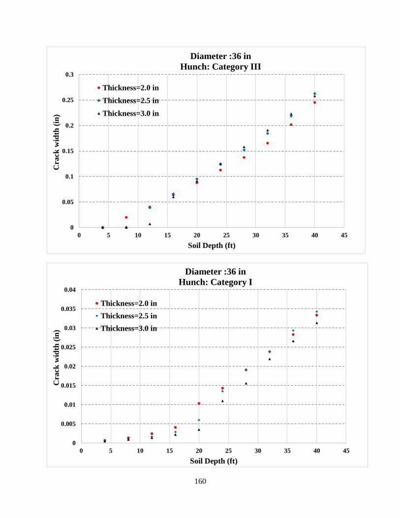
160
0
0.05
0.1
0.15
0.2
0.25
0.3
0 5 10 15 20 25 30 35 40 45
Cra
ck w
idth
(in
)
Soil Depth (ft)
Diameter :36 in
Hunch: Category III
Thickness=2.0 in
Thickness=2.5 in
Thickness=3.0 in
0
0.005
0.01
0.015
0.02
0.025
0.03
0.035
0.04
0 5 10 15 20 25 30 35 40 45
Cra
ck w
idth
(in
)
Soil Depth (ft)
Diameter :36 in
Hunch: Category I
Thickness=2.0 in
Thickness=2.5 in
Thickness=3.0 in
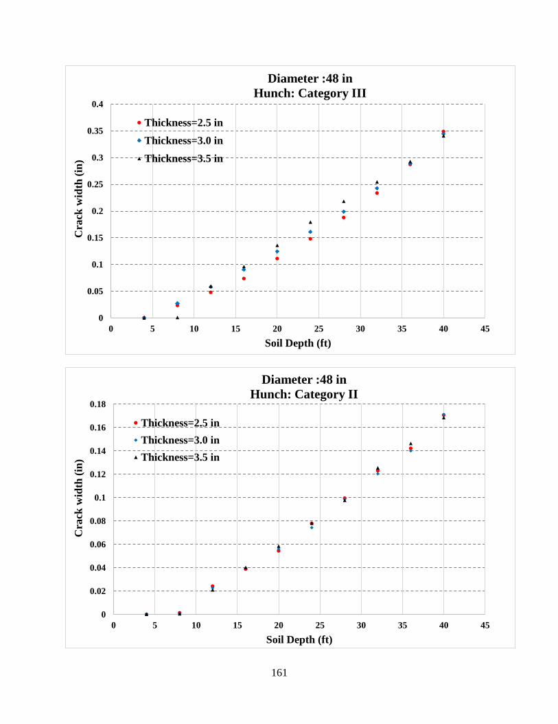
161
0
0.05
0.1
0.15
0.2
0.25
0.3
0.35
0.4
0 5 10 15 20 25 30 35 40 45
Cra
ck w
idth
(in
)
Soil Depth (ft)
Diameter :48 in
Hunch: Category III
Thickness=2.5 in
Thickness=3.0 in
Thickness=3.5 in
0
0.02
0.04
0.06
0.08
0.1
0.12
0.14
0.16
0.18
0 5 10 15 20 25 30 35 40 45
Cra
ck w
idth
(in
)
Soil Depth (ft)
Diameter :48 in
Hunch: Category II
Thickness=2.5 in
Thickness=3.0 in
Thickness=3.5 in
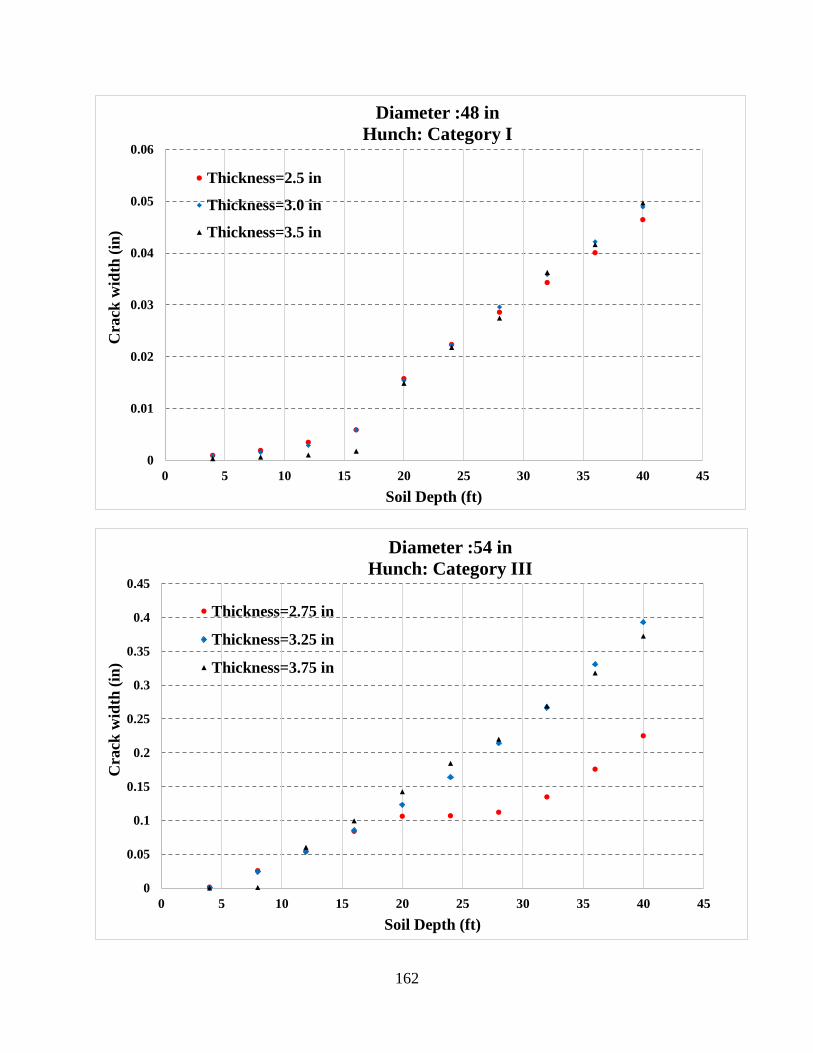
162
0
0.01
0.02
0.03
0.04
0.05
0.06
0 5 10 15 20 25 30 35 40 45
Cra
ck w
idth
(in
)
Soil Depth (ft)
Diameter :48 in
Hunch: Category I
Thickness=2.5 in
Thickness=3.0 in
Thickness=3.5 in
0
0.05
0.1
0.15
0.2
0.25
0.3
0.35
0.4
0.45
0 5 10 15 20 25 30 35 40 45
Cra
ck w
idth
(in
)
Soil Depth (ft)
Diameter :54 in
Hunch: Category III
Thickness=2.75 in
Thickness=3.25 in
Thickness=3.75 in
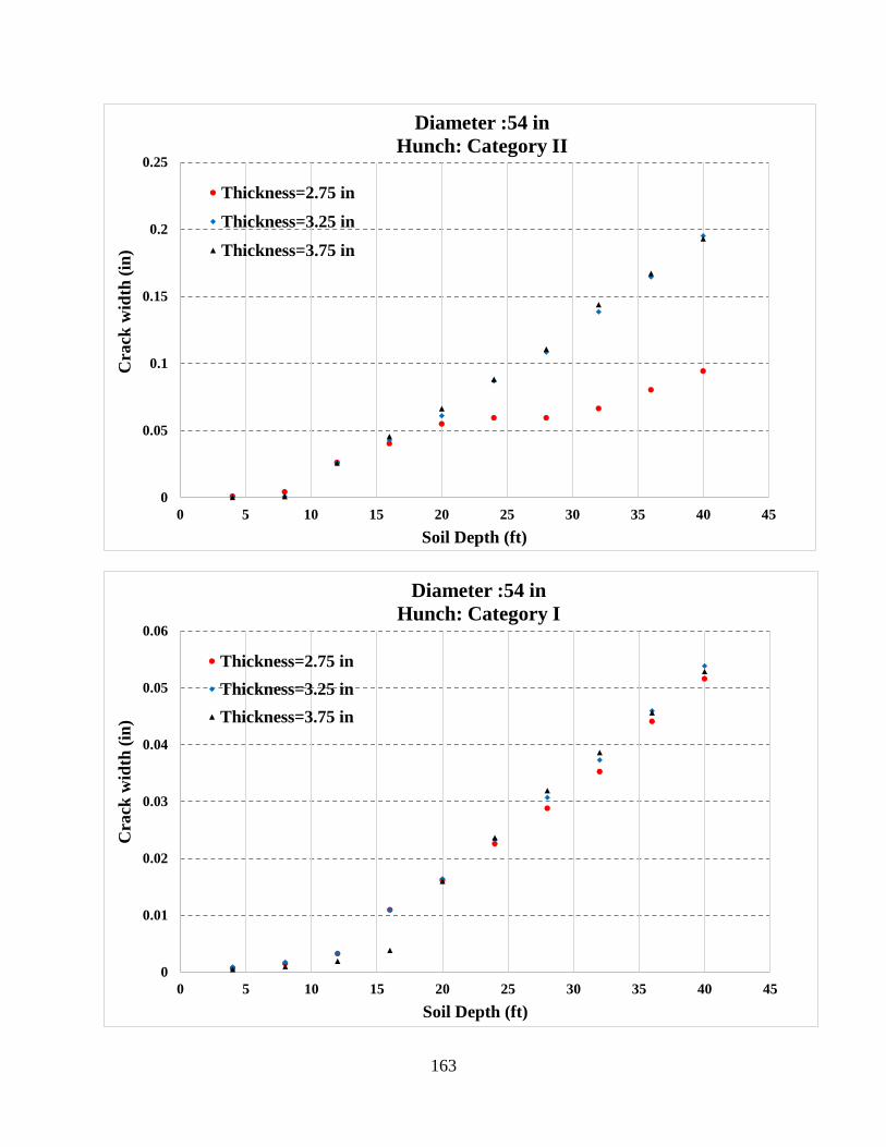
163
0
0.05
0.1
0.15
0.2
0.25
0 5 10 15 20 25 30 35 40 45
Cra
ck w
idth
(in
)
Soil Depth (ft)
Diameter :54 in
Hunch: Category II
Thickness=2.75 in
Thickness=3.25 in
Thickness=3.75 in
0
0.01
0.02
0.03
0.04
0.05
0.06
0 5 10 15 20 25 30 35 40 45
Cra
ck w
idth
(in
)
Soil Depth (ft)
Diameter :54 in
Hunch: Category I
Thickness=2.75 in
Thickness=3.25 in
Thickness=3.75 in
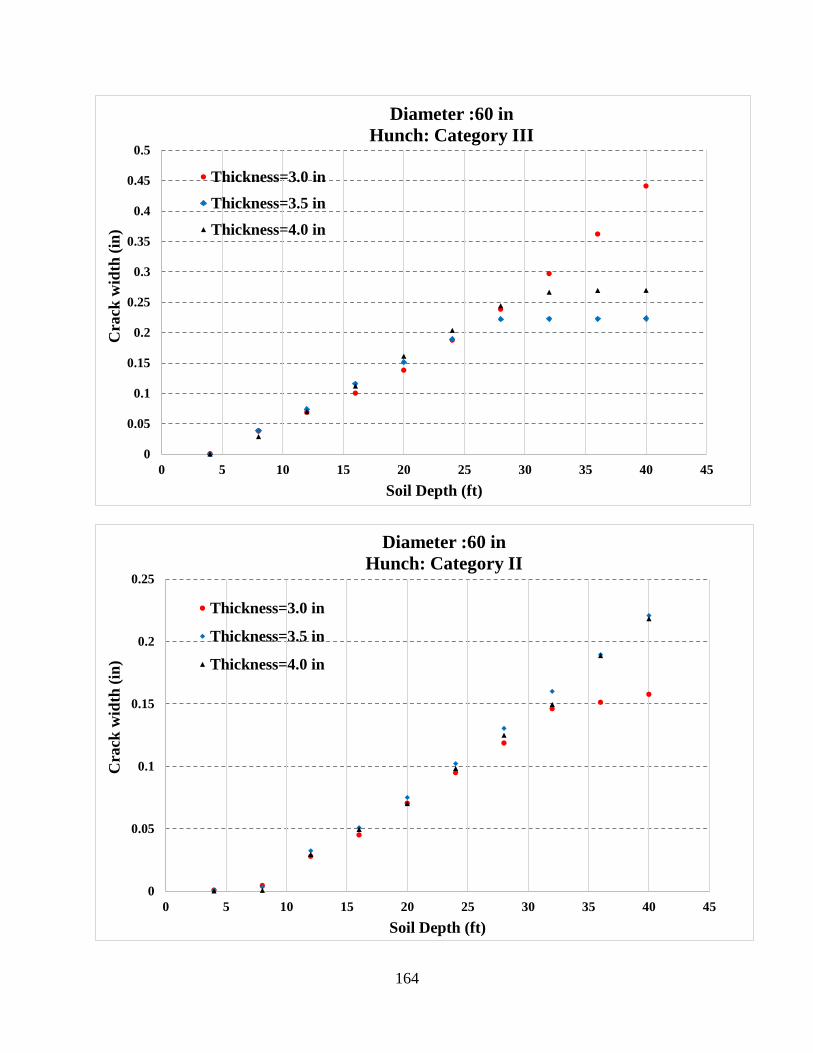
164
0
0.05
0.1
0.15
0.2
0.25
0.3
0.35
0.4
0.45
0.5
0 5 10 15 20 25 30 35 40 45
Cra
ck w
idth
(in
)
Soil Depth (ft)
Diameter :60 in
Hunch: Category III
Thickness=3.0 in
Thickness=3.5 in
Thickness=4.0 in
0
0.05
0.1
0.15
0.2
0.25
0 5 10 15 20 25 30 35 40 45
Cra
ck w
idth
(in
)
Soil Depth (ft)
Diameter :60 in
Hunch: Category II
Thickness=3.0 in
Thickness=3.5 in
Thickness=4.0 in
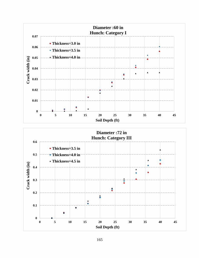
165
0
0.01
0.02
0.03
0.04
0.05
0.06
0.07
0 5 10 15 20 25 30 35 40 45
Cra
ck w
idth
(in
)
Soil Depth (ft)
Diameter :60 in
Hunch: Category I
Thickness=3.0 in
Thickness=3.5 in
Thickness=4.0 in
0
0.1
0.2
0.3
0.4
0.5
0.6
0 5 10 15 20 25 30 35 40 45
Cra
ck w
idth
(in
)
Soil Depth (ft)
Diameter :72 in
Hunch: Category III
Thickness=3.5 in
Thickness=4.0 in
Thickness=4.5 in

166
0
0.05
0.1
0.15
0.2
0.25
0.3
0 5 10 15 20 25 30 35 40 45
Cra
ck w
idth
(in
)
Soil Depth (ft)
Diameter :72 in
Hunch: Category II
Thickness=3.5 in
Thickness=4.0 in
Thickness=4.5 in
0
0.01
0.02
0.03
0.04
0.05
0.06
0.07
0.08
0 5 10 15 20 25 30 35 40 45
Cra
ck w
idth
(in
)
Soil Depth (ft)
Diameter :72 in
Hunch: Category I
Thickness=3.5 in
Thickness=4.0 in
Thickness=4.5 in
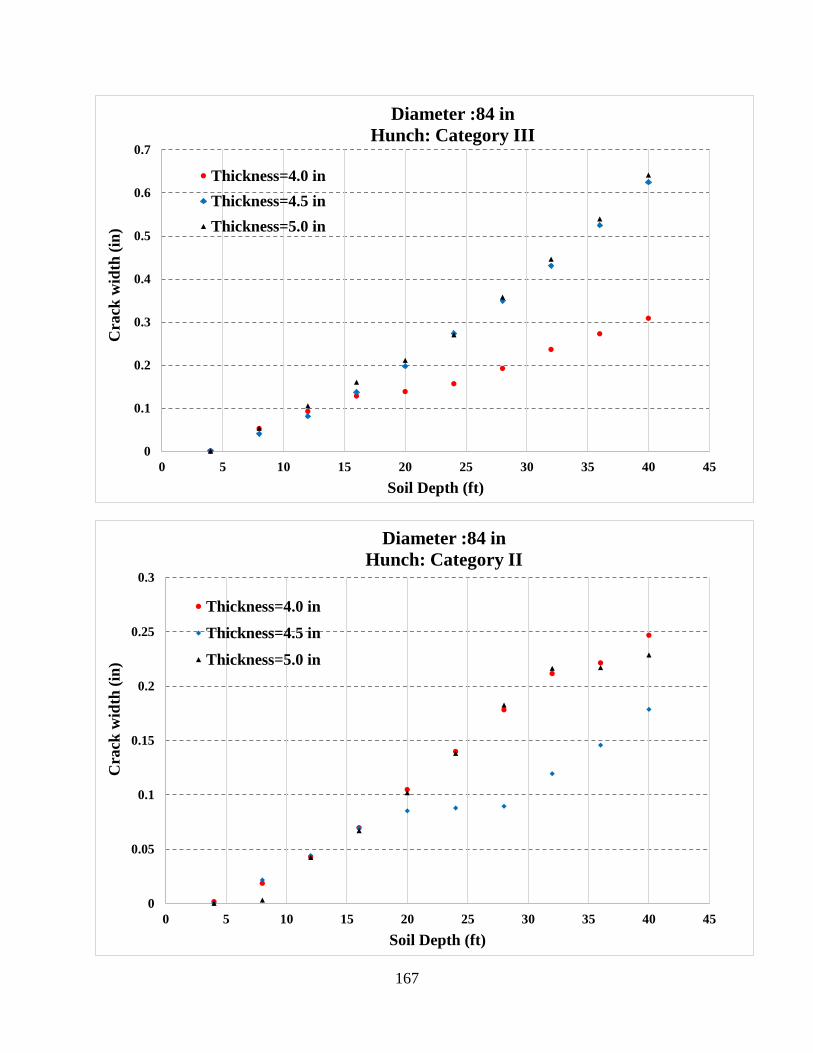
167
0
0.1
0.2
0.3
0.4
0.5
0.6
0.7
0 5 10 15 20 25 30 35 40 45
Cra
ck w
idth
(in
)
Soil Depth (ft)
Diameter :84 in
Hunch: Category III
Thickness=4.0 in
Thickness=4.5 in
Thickness=5.0 in
0
0.05
0.1
0.15
0.2
0.25
0.3
0 5 10 15 20 25 30 35 40 45
Cra
ck w
idth
(in
)
Soil Depth (ft)
Diameter :84 in
Hunch: Category II
Thickness=4.0 in
Thickness=4.5 in
Thickness=5.0 in
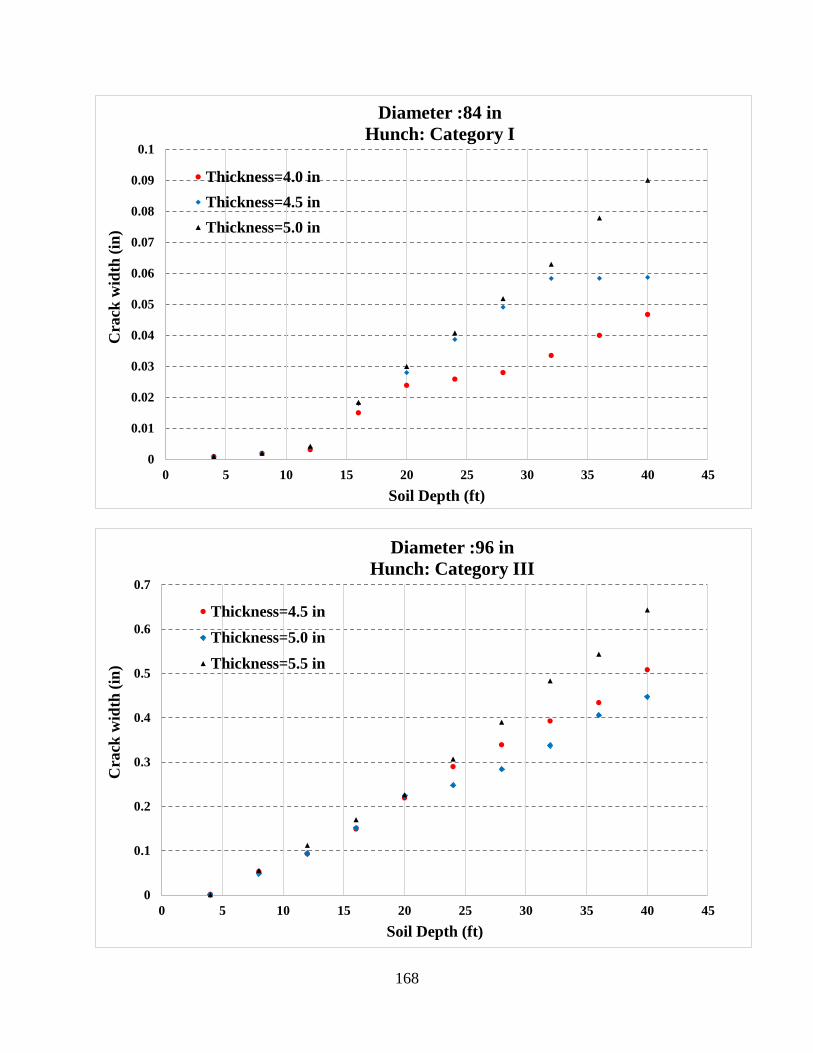
168
0
0.01
0.02
0.03
0.04
0.05
0.06
0.07
0.08
0.09
0.1
0 5 10 15 20 25 30 35 40 45
Cra
ck w
idth
(in
)
Soil Depth (ft)
Diameter :84 in
Hunch: Category I
Thickness=4.0 in
Thickness=4.5 in
Thickness=5.0 in
0
0.1
0.2
0.3
0.4
0.5
0.6
0.7
0 5 10 15 20 25 30 35 40 45
Cra
ck w
idth
(in
)
Soil Depth (ft)
Diameter :96 in
Hunch: Category III
Thickness=4.5 in
Thickness=5.0 in
Thickness=5.5 in
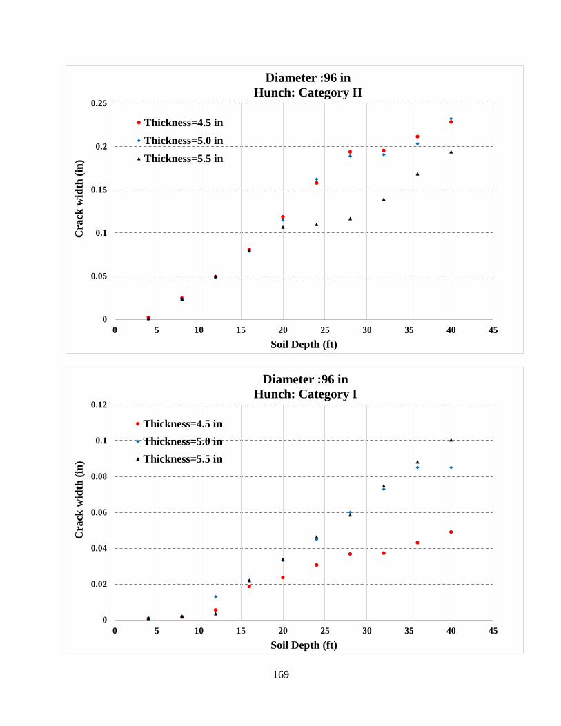
169
0
0.05
0.1
0.15
0.2
0.25
0 5 10 15 20 25 30 35 40 45
Cra
ck w
idth
(in
)
Soil Depth (ft)
Diameter :96 in
Hunch: Category II
Thickness=4.5 in
Thickness=5.0 in
Thickness=5.5 in
0
0.02
0.04
0.06
0.08
0.1
0.12
0 5 10 15 20 25 30 35 40 45
Cra
ck w
idth
(in
)
Soil Depth (ft)
Diameter :96 in
Hunch: Category I
Thickness=4.5 in
Thickness=5.0 in
Thickness=5.5 in
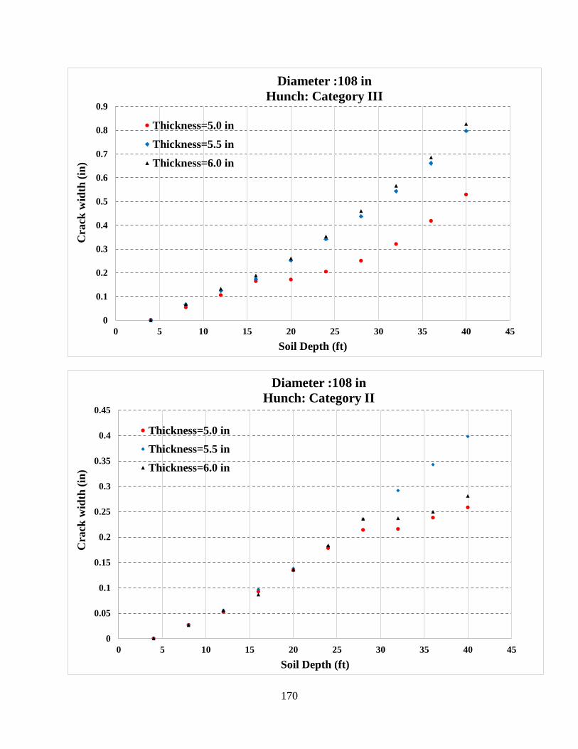
170
0
0.1
0.2
0.3
0.4
0.5
0.6
0.7
0.8
0.9
0 5 10 15 20 25 30 35 40 45
Cra
ck w
idth
(in
)
Soil Depth (ft)
Diameter :108 in
Hunch: Category III
Thickness=5.0 in
Thickness=5.5 in
Thickness=6.0 in
0
0.05
0.1
0.15
0.2
0.25
0.3
0.35
0.4
0.45
0 5 10 15 20 25 30 35 40 45
Cra
ck w
idth
(in
)
Soil Depth (ft)
Diameter :108 in
Hunch: Category II
Thickness=5.0 in
Thickness=5.5 in
Thickness=6.0 in
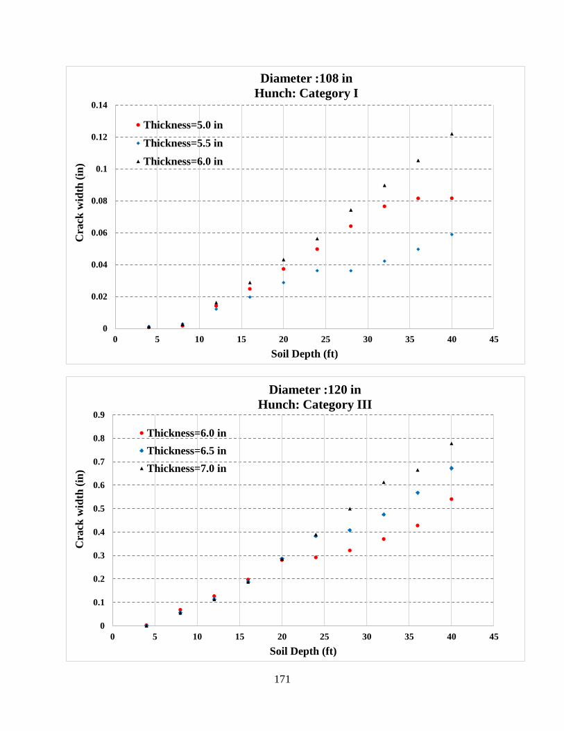
171
0
0.02
0.04
0.06
0.08
0.1
0.12
0.14
0 5 10 15 20 25 30 35 40 45
Cra
ck w
idth
(in
)
Soil Depth (ft)
Diameter :108 in
Hunch: Category I
Thickness=5.0 in
Thickness=5.5 in
Thickness=6.0 in
0
0.1
0.2
0.3
0.4
0.5
0.6
0.7
0.8
0.9
0 5 10 15 20 25 30 35 40 45
Cra
ck w
idth
(in
)
Soil Depth (ft)
Diameter :120 in
Hunch: Category III
Thickness=6.0 in
Thickness=6.5 in
Thickness=7.0 in
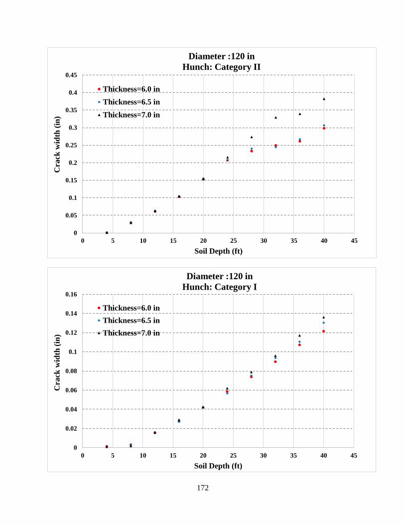
172
0
0.05
0.1
0.15
0.2
0.25
0.3
0.35
0.4
0.45
0 5 10 15 20 25 30 35 40 45
Cra
ck w
idth
(in
)
Soil Depth (ft)
Diameter :120 in
Hunch: Category II
Thickness=6.0 in
Thickness=6.5 in
Thickness=7.0 in
0
0.02
0.04
0.06
0.08
0.1
0.12
0.14
0.16
0 5 10 15 20 25 30 35 40 45
Cra
ck w
idth
(in
)
Soil Depth (ft)
Diameter :120 in
Hunch: Category I
Thickness=6.0 in
Thickness=6.5 in
Thickness=7.0 in
173
REFERENCES
[1] Shook, W. E., and Bell, L. W., “Corrosion Control in Concrete Pipe and Manholes,” Technical
Presentation, Water Environmental Federation, Orlando, FL, 1998, pp. 1-5.
[2] American Concrete Pipe Association (ACPA), “Concrete Pipe Design Manual: Revised to
Include Standard Installations”, Irving, TX, 2005
[3] ASTM, Standard specification for reinforced concrete culvert, storm drain, and sewer pipe,
C76-14, 04.05, American Society for testing and Materials, West Conshohocken, PA;2014.
[4] Moser A. P., Buried Pipe Design, 2ed, New York, McGraw-Hill, 2001
[5] AASHTO M 294-11, “Standard Specification for Corrugated Polyethylene Pipe, 300- to 1500-
mm (12- to 60-in.) Diameter”
[6] ASTM, “Standard Test Method for Determination of External Loading Characteristics of
Plastic Pipe by Parallel-Plate Loading”, D2412-11, 08.04, American Society for testing and
Materials, West Conshohocken, PA; 2011.
[7] ASTM, “Standard Specification for Corrugated Polyethylene (PE) Pipe and Fittings”, F405-
13, 08.04, American Society for testing and Materials, West Conshohocken, PA; 2013.
[8] Spangler, M. G. “The supporting strength of rigid pipe culverts”. Iowa Engineering Experiment
Bulletin Vol.112, 1933.
[9] ASTM, Standard Test Methods for Concrete Pipe, Manhole Sections, or Tile, C497-19,
American Society for testing and Materials, West Conshohocken, PA;2019.
[10] Heger, Frank J., and Timothy J. McGrath. "Design method for reinforced concrete pipe and
box sections." (1982).
[11] AASHTO L.R.F.D, “Bridge Design Specifications” Section 12, American Association of
State Highway and Transportation Officials, Washington DC. (2012)
174
[12] A. Wilson and A. Abolmaali, “Comparison of Material Behavior of Steel and Synthetic Fibers
in Dry-Cast Application,” Transp. Res. Rec. J. Transp. Res. Board, vol. 2332, no. 1, pp. 23–28,
2013.
[13] A. M. Alhozaimy, P. Soroushian, and F. Mirza, “Mechanical properties of polypropylene
fiber reinforced concrete and the effects of pozzolanic materials,” Cem. Concr. Compos., vol. 18,
no. 2, pp. 85–92, 1996.
[14] P. S. Song, S. Hwang, and B. C. Sheu, “Strength properties of nylon- and polypropylene-
fiber-reinforced concretes,” Cem. Concr. Res., vol. 35, no. 8, pp. 1546–1550, 2005.
[15] S. Kurtz and P. Balaguru, “Postcrack creep of polymeric fiber-reinforced concrete in flexure,”
Cem. Concr. Res., vol. 30, no. 2, pp. 183–190, 2000.
[16] K. Ari, O. Karahan, C. D. Atis, C. Bilim, and Ö. C. Sola, “Relation between Strength
Properties (Flexural and Compressive) and Abrasion Resistance of Fiber (Steel and
Polypropylene)-Reinforced Fly Ash Concrete,” Aug. 2009.
[17] Park, Yeonho, et al. "Time-Dependent Behavior of Synthetic Fiber–Reinforced Concrete
Pipes Under Long-Term Sustained Loading." Transportation Research Record 2407.1 (2014): 71-
79
[18] de la Fuente, Albert, et al. "Design of macro-synthetic fibre reinforced concrete pipes."
Construction and Building Materials 43 (2013): 523-532.
[19] Peyvandi, Amirpasha, Parviz Soroushian, and Shervin Jahangirnejad. "Enhancement of the
structural efficiency and performance of concrete pipes through fiber reinforcement." Construction
and Building Materials 45 (2013): 36-44.
[20] Mostafazadeh, Mahnaz, and Ali Abolmaali. "Shear behavior of synthetic fiber reinforced
concrete." Advances in Civil Engineering Materials 5.1 (2016): 371-386.
175
[21] J. R. Roesler, D. a. Lange, S. a. Altoubat, K.-A. Rieder, and G. R. Ulreich, “Fracture of Plain
and Fiber-Reinforced Concrete Slabs under Monotonic Loading,” J. Mater. Civ. Eng., vol. 16, no.
5, pp. 452–460, 2004.
[22] Ghahremannejad, Masoud, Maziar Mahdavi, Arash Emami Saleh, Sina Abhaee, and Ali
Abolmaali. "Experimental investigation and identification of single and multiple cracks in
synthetic fiber concrete beams." Case Studies in Construction Materials 9 (2018): e00182.
[23] N. Van Chanh, “Steel fiber reinforced concrete,” Construction, vol. 25, no. 1, pp. 108–116,
2004.
[24] Katona, M. G., et al. CANDE--A Modern Approach for the Structural Design and Analysis
of Buried Culverts. No. FHWA-RD-77-5 Final Rpt. 1976.
[25] Heger, Frank J., Atis A. Liepens, and Ernest T. Selig. "SPIDA: An analysis and design system
for buried concrete pipe." Advances in underground pipeline engineering. ASCE, 1985.
[26] Kang, Junsuk, Frazier Parker, and Chai H. Yoo. "Soil-structure interaction and imperfect
trench installations for deeply buried concrete pipes." Journal of geotechnical and
geoenvironmental engineering 133.3 (2007): 277-285.
[27] Abolmaali, Ali, and Anupong Kararam. "Nonlinear finite-element modeling analysis of soil-
pipe interaction." International Journal of Geomechanics 13.3 (2011): 197-204
[28] Zhang, J., D. P. Stewart, and M. F. Randolph. "Kinematic hardening model for pipeline-soil
interaction under various loading conditions." The International Journal of Geomechanics 2.4
(2002): 419-446.
[29] Tian, Yinghui, and Mark J. Cassidy. "Modeling of pipe–soil interaction and its application in
numerical simulation." International Journal of Geomechanics 8.4 (2008): 213-229.
176
[30] Srivastava, Amit, Chaitanya R. Goyal, and Abhishek Raghuvanshi. "Load settlement response
of footing placed over buried flexible pipe through a model plate load test." International Journal
of Geomechanics 13.4 (2012): 477-481.
[31] Zarghamee, Mehdi S., and David B. Tigue. Soil-Structure interaction of flexible pipe under
pressure. No. 1087. 1986.
[32] Suleiman, Muhannad T., et al. "Analysis of deeply buried flexible pipes." Transportation
research record 1849.1 (2003): 124-134.
[33] McGrath, Timothy J. "Pipe-soil interactions during backfill placement." (1998).
[34] Salehi Dezfooli, Mojtaba. "Staged Construction Modeling Of Large Diameter Steel Pipes
Using 3-D Nonlinear Finite Element Analysis." (2016).
[35] Sharma, Jwala Raj, et al. "Testing and evaluation of statically-loaded large diameter steel pipe
with native backfill soils." Pipelines 2011: A Sound Conduit for Sharing Solutions. 2011. 1025-
1034.
[36] A. Hillerborg, M. Modéer, and P.-E. Petersson, “Analysis of crack formation and crack
growth in concrete by means of fracture mechanics and finite elements,” Cem. Concr. Res., vol.
6, no. 6, pp. 773–781, 1976.
[37] A. Hillerborg, “The theoretical basis of a method to determine the fracture energy GF of
concrete,” Mater. Struct., vol. 18, no. 106, pp. 291–296, 1985.
[38] Y. R. Rashid, “Ultimate strength analysis of prestressed concrete pressure vessels,” Nucl.
Eng. Des., vol. 7, no. 4, pp. 334–344, 1968.
[39] O. Hemmy, “Recommendations for finite element analysis of FRC`, report of subtask 3.5,
Brite-EuRam Project BRPR-CT98-0813: Test and design methods for steel fibre reinforced
177
concrete, project funded by the European Community under the Industrial & Materials Technolo,”
2002.
[40] J. Lubliner, J. Oliver, S. Oller, and E. Oñate, “A plastic-damage model for concrete,” Int. J.
Solids Struct., vol. 25, no. 3, pp. 299–326, 1989.
[41] J. Lee and G. L. Fenves, “Plastic-Damage Model for Cyclic Loading of Concrete Structures,”
Aug. 1998.
[42] A. S. Genikomsou and M. A. Polak, “Finite element analysis of punching shear of concrete
slabs using damaged plasticity model in ABAQUS,” Eng. Struct., vol. 98, pp. 38–48, 2015.
[43] Brinkgreve, Ronald BJ. "Selection of soil models and parameters for geotechnical engineering
application." ASCE, (2005.)
[44] ABAQUS 6.14 Documentation. 2016. ABAQUS Manual, version 6.14, Pawtucket, R.I.
[45] AASHTO M 294-11, “Standard Specification for Corrugated Polyethylene Pipe, 300- to
1500-mm (12- to 60-in.) Diameter”
[46] ASTM, “Standard Test Method for Determination of External Loading Characteristics of
Plastic Pipe by Parallel-Plate Loading”, D2412-11, 08.04, American Society for testing and
Materials, West Conshohocken, PA; 2011.
[47] S. Y. Alam, J. Saliba, and A. Loukili, “Study of evolution of fracture process zone in concrete
by simultaneous application of digital image correlation and acoustic emission,” VIII Int. Conf.
Fract. Mech. Concr. Concr. Struct., no. FraMCoS-8, pp. 1–9, 2012.
[48] B. Pan, K. Qian, H. Xie, and A. Asundi, “Two-dimensional digital image correlation for in-
plane displacement and strain measurement: a review,” Meas. Sci. Technol., vol. 20, no. 6, p.
62001, 2009.
178
[49] H. Lu and P. D. Cary, “Deformation measurements by digital image correlation:
Implementation of a second-order displacement gradient,” Exp. Mech., vol. 40, no. 4, pp. 393–
400, 2000.
[50] RILEM TC 162-TDF, “Final recommendation of RILEM TC 162-TDF: Test and design
methods for steel fiber reinforced concrete sigma-epsilon-design method,” Mater. Struct., vol. 36,
no. 262, pp. 560–567, 2003.
[51] C. C. Test, T. Drilled, C. Concrete, and S. T. Panels, “C 1609/C 1609M-05 Standard Test
Method for Flexural Performance of Fiber-Reinforced Concrete (Using Beam with Third-Point
Loading) 1,” ASTM, vol. I, no. C 1609/C 1609M-05, pp. 1–8, 2005.
[52] C. C. Test, T. Drilled, and C. Concrete, “Standard Test Method for Flexural Strength of
Concrete (Using Simple Beam with Third-Point Loading) 1,” Hand, vol. C78-2, no. C, pp. 1–4,
2010
[53] “GOM Correlate user manual v6.” GOM mbH, Germany, 2016
[54] “ABAQUS Analysis user’s manual 6.14-EF.” Dassault Systems Simulia Corp, Providence,
RI, USA, 2014.
[55] J. Y. Wu, J. Li, and R. Faria, “An energy release rate-based plastic-damage model for
concrete,” Int. J. Solids Struct., vol. 43, no. 3, pp. 583–612, 2006.
[56] G. Voyiadjis and Z. Taqieddin, “Elastic Plastic and Damage Model for Concrete Materials:
Part I-Theoretical Formulation,” Int. J. Struct. Chang. Solids, vol. 1, no. 1, pp. 31–59, 2009.
[57] A. S. Genikomsou and M. A. Polak, “Finite element analysis of punching shear of concrete
slabs using damaged plasticity model in ABAQUS,” Eng. Struct., vol. 98, pp. 38–48, 2015.
179
[58] S.-T. Kang, Y. Lee, Y.-D. Park, and J.-K. Kim, “Tensile fracture properties of an Ultra High-
Performance Fiber Reinforced Concrete (UHPFRC) with steel fiber,” Compos. Struct., vol. 92, no.
1, pp. 61–71, 2010.
[59] Selig, Ernest T. "soil properties for plastic pipe installations." Buried Plastic Pipe Technology
1 (1990): 141