On the determination of the absolute unit of resistance by ...rspa.royalsocietypublishing.org/content/royprsa/87/597/391.full.pdf · Standard Mutual Inductance ... = 0-03296, = 0-07002

391

On the Determination o f the Absolute Unit o f Resistance byAlternating Current Methods.

By Albert Campbell, B.A.

(Communicated by R. T. Glazebrook, F.R.S. Received July 2, 1912.)

(From the National Physical Laboratory.)

CONTENTS.PAGE

1. Introductory ............................................ 3912. Standard Mutual Inductance ............................................................. 3913. Secondary Standard : Mutual Inductometer ...................................... 3964. Comparison of Resistance and Mutual Inductance by Two-phase

Method ............................ 3985. Method of Intermediary Condenser ..................................................... 402

1. Introductory.—Kecently at the National Physical Laboratory we have constructed a standard of mutual inductance of novel type, whose value has been accurately calculated from the dimensions. This inductance has formed the basis for the determination of the unit of resistance in absolute measure by two different methods, in both of which alternating current is employed. Although there is no doubt that the accuracy attainable by these methods could be increased by greater elaboration of the apparatus used, the results already obtained seem to be of sufficient interest to warrant publication. I t should be mentioned that the accuracy here aimed at was of a considerably lower order than that contemplated in the determination of the ohm by the Lorenz apparatus which is at present being carried out in the laboratory. For the experiments here described, no apparatus was specially constructed, but use was made of instruments which had already been designed and set up for the measurement of inductance and capacity. I shall first give a brief description of the standard inductance and then pass on to the methods and results.

2. Standard Mutual Inductance.—The design of the mutual inductance has already been described.* The electrical circuits have the form and arrangement shown in section in fig. 1.

The primary circuit consists of two single-layer coils C and D connected in series, while the secondary is a coil H of many layers wound in a comparatively narrow channel.

The dimensions and positions of the coils are such that the magnetic field due to current in C and D is practically zero over the space occupied by the

* ‘Roy. Soc. Proc.,’ May, 1907, A, vol. 79, p. 428.

on April 30, 2018http://rspa.royalsocietypublishing.org/Downloaded from

http://rspa.royalsocietypublishing.org/

392 Mr. A. Campbell. Absolute Unit o f [July 2,

windings of H. Thus (a) the calculation of the mutual inductance M can be made with accuracy without an accurate knowledge of the dimensions of the many-layered coil H, provided the dimensions of C and D can be accurately

F ig. 1.

measured; (b) slight eccentric or axial displacements of the coil H from the symmetrical position have very small effect on the value of M, and hence the setting of H into its proper position can be done without difficulty. The actual construction is shown in fig. 2.

The coils C and D consisted of bare hard copper wire (diameter 0*6 mm.) wound in right and left handed screw threads cut on a single white marble cylinder, the pitch of the screw being 1 mm. The treatment of the marble and the process of winding of these coils were very similar to those used by Mr. F. E. Smith in the construction of the standard ampere balance,* and need not be further described here. The same remark applies to the measurement of the dimensions of the coils C and D, which was carried out by Mr. L. F. Richardson, of the Metrology Department. As the distance from wire to wire of the winding was about 0*4 mm. it was not considered necessary to employ bifilar winding. After winding, the coils were dipped in melted paraffin wax. The leads were led out parallel to the axis and almost touching the outer surface of the winding. The coil H was of nearly square section and was wound of double silk covered copper wire (diameter 0*385 mm.) in a channel accurately turned in a large white marble ring, supported by a ring of built mahogany having three solid ebonite feet and provided with screws by which the level and centrality could be independently adjusted. The main part of coil H was in four nearly equal sections brought

* 4 Phil. Trans.,5 A, vol. 207.



out to separate leads and having 97, 145, 145, and 98 turns respectively. A thin strip of paper was interposed between each layer and the whole was well soaked in melted paraffin after winding. An auxiliary coil (for 1 millihenry) was wound over the main coil; it was not, however, used in the present experiments. Outside of this was wound a single turn which was connected in series with the main coil so as to make the total value of the mutual inductance almost exactly lO'OO millihenries.

During winding, the number of turns was recorded by a counter, and when

1912.] Resistance by Alternating Current Methods. 393

F ig. 2.

the coil was complete, the accuracy of the counting and the sufficiency of the insulation were checked by separately measuring the mutual inductance of each section, using C and D as primary. During the winding the girth of each layer was tested by a carefully calibrated steel tape.

The dimensions at 15° C. were as follows :—Coils C and D.—75 turns each. Mean diameter, 30’005i cm. Distance

between inner ends of coils, 14-99965 cm.; between outer ends, 29-9967 cm.Main Coil H.—485 turns. Mean diameter, 43‘7374 cm. Axial depth,

l ’OOo cm. Radial depth, 0'86i cm.



394

The calculation of the mutual inductance was made in the following manner. To begin with, an arrangement of coils (C0, D0, and H 0) was chosen, having the dimensions of C and 1) round numbers; for convenience I shall refer to C, D, H as “ the model,” although it was not actually constructed. The dimensions as shown in fig. 1 were A = 10, = 5, and = 10 cm.respectively. The mean radius of the main coil was chosen so as to give maximum mutual inductance between its central filament and the coils C0 and D0. This was done as already described* by calculating the mutual inductances between C and D connected in series and a series of circles midway between them of radii 14*1, 14-3, 14-5, 14’7 and 14'9 cm. respectively.

The results of the more accurate recalculation are given in Table I, NiNj, the product of primaiy and secondary turns, being taken as 100,000. In the last column are given the corresponding values of 3M/3

Mr. A. Campbell. Absolute Unit o f [July 2,

Table I.A = 10 cm., b = 5 to 10 cm., N"iN"2 = 100,000.

a. M. 0M/0 a.

cm. millihenries.14 *1 9 *1631 + 0 *0559514 -3 9 -17218 + 0 *0318214 *5 9 *1759 + 0*00910914 *7 9 *1754 - 0 *01240114 *9 9 ‘1696 - 0 *032148

If £ = a —14-583, then from the numbers in the table we find

~ = -0 -1 0 7 6 7 f+ 0-01648 p+0-01167 P + 0 0 2 0 3CiCi

Hence M is a maximum for variation of when a 14-583; also, when £ = 0, we have

= -0-10767, = 0-03296, = 0-07002.

For a = 14-583, the maximum value M0 = 9T7624.

Integration over Cross-section of Main Coil.—The mean radius of the actual main coil is 21-8687 cm. When this is reduced by dividing by 1"5 to correspond with the model we have «0 = 14-579i. As the variation of M with a is very small, this value may be taken as a close enough approximation to 14-583, the value giving maximum M. This maximum (M0) refers to a single circle, the central filament of the rectangular cross-section of the

* Loc. cit.



395

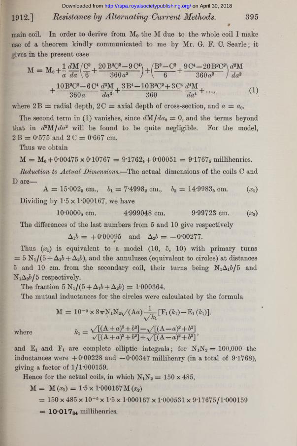
main coil. In order to derive from M0 the M due to the whole coil I make use of a theorem kindly communicated to me by Mr. G. F. C. Searle; it gives in the present case

1912.] Resistance by Alternating Current Methods.

M ld M ( C 2 20B2C2- 9 C 4\ /B2- C 2 9C4- 2 0 B 2C2W 2M a da \T) 360a2 / + \ 6 + 360a2 / da2

10B2C2—6C4 # M 3B4- 1 0 B 2C2 + 3C4 #M 360 a da? 360 ffa4 ’ (1)

where 2B = radial depth, 2C = axial depth of cross-section, and a = a0.

The second term in (1) vanishes, since dM /da0 = 0, and the terms beyond that in d2M /da2 will be found to be quite negligible. For the model, 2 B = 0575 and 2 C = 0667 cm.

Thus we obtain

M = M0 + 0-00 4 75 x 0-107 67 = 9\L7624 + 000051 = 9-l767s millihenries.Reduction to Actual Dimensions.—The actual dimensions of the coils C and

D are—A = 15'0025 cm., b\ = 7"49982 cm., = 14"99835 cm.

Dividing by l -5 x 1-000167, we have

10-0000o cm. 4-999048 cm. 9-99723 cm.The differences of the last numbers from 5 and 10 give respectively

Ai&= +0-00095 and A26 = -0-00277.#Thus ( Xi) is equivalent to a model (10, 5, 10) with primary turns

= 5 Ni/(5 + Ai& + A2&), and the anniduses (equivalent to circles) at distances 5 and 10 cm. from the secondary coil, their turns being NiAi&/5 and N iA2&/5 respectively.

The fraction 5 Ni/(5 + A ^ + A2b) = 1-000364.The mutual inductances for the circles were calculated by the formula

where

M = 10-9x 8 7rN1N2x/( A a ) - L .[ F 1(A;1) - E 1(*1)],V ^1

Jc = x /[(A + a)2 + &21 - ^ / [ ( A - a ) 2 + 52]1 +[(A + a)2 + S2] + x/ [ ( A - a ) 2 + 62] ’

and Ei and Fi are complete elliptic integrals; for N iN2 = 100,000 the inductances were +0*00228 and —0*00347 millihenry (in a total of 9*1768), giving a factor of 1/1*000159.

Hence for the actual coils, in which NiN2 = 150 x 485,M = M (^ ) = 1*5 x 1*000167 M (#2)

= 150 x 485 x 10-* x 1*5 x 1*000167 x 1*000531 x 9*17675/1*000159 = 1 0 -0 1 7 84 millihenries.



396

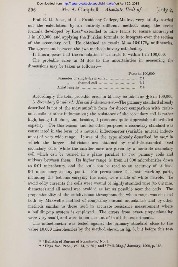
Prof. R. LI. Jones, of the Presidency College, Madras, very kindly carried out the calculation by an entirely different method, using the series formula developed by Rosa* extended to nine terms to ensure accuracy of 1 in 100,000, and applying the Purkiss formula to integrate over the section of the secondary coil. He obtained as result M = 10*01782 millihenries. The agreement between the two methods is very satisfactory.

I t thus appears that the calculation is accurate to within 1 in 100,000.The probable error in M due to the uncertainties in measuring the

dimensions may be taken as follows:—

Parts in 100,000.


Diameter of single-layer co ils................................ ±1„ channel coil ........................................ ± 2

Axial len gth s............................................................. ± 4

Accordingly the total probable error in M may be taken as ± 5 in 100,000.3. Secondary Standard: Mutual Inductometer.—The primary standard already

described is not of the most suitable form for direct comparison with resistance coils or other inductances; the resistance of the secondary coil is rather high, being 140 ohms, and, besides, it possesses quite appreciable distributed capacity. For this reason and for other purposes a secondary standard was constructed in the form of a mutual inductometer (variable mutual inductance) of very wide range. I t was of the type already described by me,f in which the larger subdivisions are obtained by multiple-stranded fixed secondary coils, while the smaller ones are given by a movable secondary coil which can be turned in a plane parallel to two primary coils and midway between them. Its higher range is from 11,000 microhenries down to 0*01 microhenry, and the scale can be read to an accuracy of at least 0*1 microhenry at any point. For permanence the main working parts, including the bobbins carrying the coils, were made of white marble. To avoid eddy currents the coils were wound of highly stranded wire (to 0*2 mm. diameter) and all metal was avoided as far as possible near the coils. The proportionality of the subdivisions throughout the whole range was checked both by Maxwell's method of comparing mutual inductances and by other methods similar to those used in accurate resistance measurement where a building-up system is employed. The errors from exact proportionality were very small, and were taken account of in all the experiments.

The inductometer was tested against the primary standard close to the value 10,000 microhenries by the method shown in fig. 3, but before this test

* 4 Bulletin of Bureau of Standards,5 No. 3.t 4 Phys. Soc. Proc.,’ vol. 21, p. 69 ; and 4 Phil. Mag.,5 January, 1908, p. 155.



1912.] Resistance by Alternating Methods. 397

the secondary coil of the primary standard (I) was adjusted to be (a) exactly midway between the two primary coils, and coaxial with them.

Adjustment (a) was effected by connecting the two primary coils of (I) in series but opposing one another magnetically, while the secondary was connected to a telephone. Alternating current at 800 ~ per second was passed through the primary circuit and the position of the secondary coil was adjusted until silence was reached in the telephone.

Adjustment (b) was made during the comparison with the inductometer, the relative positions of the coil-axes being altered until the minimum reading on the inductometer was obtained.

F ig. 3.

In fig. 3 the inductometer (m)and the standard (I) have their primary coils connected in series to A, a source of alternating current of frequency their secondary coils being connected in series (and opposition) to a tuned vibration galvanometer G. By varying the value of t o an approximate balance can be obtained; the want of exact balance is due to the difference in distributed capacity of the two secondaries (and of the primaries also). The balance can be made exact by adjusting a variable condenser connected across the segondary of m (in our case). If the resultant distributed capacity effects be represented by a capacity K across M, and if L, R, l, and r be the self-inductances and resistances as in the figure, and m = 27m, it is •easy to show that

M _ R K _ 1 —LKo>2 (m rk 1 — Ikw2 '

When M is nearly equal to to, we have as a sufficient approximationM/m == 1— co2k(L (3)

The actual values wereL = 0260 henry, l = 0'025i henry.R = 140 ohms, r = 17'73 ohms.

Hence (L r/R — 1) = 7'8 millihenries.



398

The comparisons were made at three frequencies. For n = 0 the alternating current was replaced by direct current with a single reversal, and the vibration galvanometer by a ballistic one. In Table I I are given the results.

Table II.


n. lc.

Error of inductometer. Parts in 100,000.

Apparent. Corrected.

~ per sec. 0

microfarad.0 + 0 *27 + 0 ‘2r

50 0*02 + 0 *45 + 0 *2s100 0*02 + 0 *85 + 0-32

The corrected values show satisfactory agreement, and thus when the inductometer reads 10000, the true value is 10000*3 microhenries.

I t was found that when a current of 1 ampere was passed through the primary circuit of the inductometer for several minutes, the slight warming of the coils caused a gradual change (of the order of 1 to 2 parts in 100,000) in the error. A small correction for this was applied when necessary in the experiments described below.

4. Comparison of Resistance and Mutual Inductance by Two-Phase Method. The most direct comparison of resistance with mutual inductance was made by the method already briefly described by me,* in which two-phase alternating currents are used.

In fig. 4, M is the inductometer, E a standard oil-cooled resistance, and G-

Fig. 4.—Two-phase Method.

* ‘ Eoy. Soc. Proc.,’ 1908, vol. 81, p. 450.




a vibration galvanometer tuned to the frequency n of the alternator. Let A cos wt and B sin a t be the instantaneous values of currents in quadrature (as shown); then if the galvanometer shows no deflection

B = ^ a ) M . (4)B

In practice A is very nearly equal to B, but R is not perfectly non-inductive. Let its self-inductance be l, causing circuit A to be slightly out of quadrature with B by a small angle %. Then for a balance (when A = B) we have

wM cos (tof + ff) —Rcos — sin = 0;or, since l is small compared with M,

wM cos cot — aM-x sin a t —R cos sin 0.Thus R = wM, as before, and x =?

If l\M is even as large as 1/1000, R will not differ from <wM by more than 1 in 2,000,000. The small phase displacement % is balanced in the adjustment of l2. The actual value of l for the coil used was 1‘6 microhenry, while M was 10,000 microhenries ; thus the correction is quite negligible.

Determination of A /B.—The ratio of A to B (which is taken very nearly equal to unity) is found by observing the effective values of the two currents by the respective potential differences .produced in the (very nearly) equal resistances r\ and r2,these voltages being read alternately on a very sensitiveelectrostatic voltmeter V. If the wave forms are not exact sine curves, the instantaneous values of the currents may be written

2A S cos (s cot + <l>s)and 2 Bs sin <£s) respectively, where s = 1, 3, 5 ...

In this case the ratio of the effective values will be(Ai2 + A32 + Aa2 + . . .)i/B!2 + B32 + B52 + . ..)*,

ie. A l ( l + as? + a!? + ...) i/B 1( l + bs*+ h2+...)t.(5)Now in the alternator used, the wave forms had been carefully traced and

it was known that (a3 + «5+ ...) and (&3 + &5+ ...) were neither of them of an order greater than 1/100 ; hence expression (5) will not differ from A /B by more than 1 part in 20,000. The error, if any, can, however, be eliminated by repeating the experiment with the coils of the alternator interchanged.

Effect of Distributed Capacity in Inductometer.—The coils of the inductometer have small distributed capacities, the total effect of which may be represented by a small capacity K across the ends of the secondary coil of self inductance L. I t is easy to show that for equation (4) we must write

R ( l —LK«2) = ^ WM. (6)B



400

The correction LKo>2 is proportional to the square of the frequency. As will be shown later, it was evaluated by testing an air condenser against the inductometer at various frequencies up to 2000 ~ per second. At 80 ~ per second, the frequency used, the correction was approximately 6 in 1,000,000.

Determination of Frequency.—By a worm and wheel connected to the alternator spindle, at every 100 revolutions an electric contact was made and this caused a record to be made by the pen of a chronograph to which at the same time the standard clock was sending signals each second. A comparison of their respective marks over a sufficiently long interval gave the average frequency.

Procedure of Experiment.—The alternator was run at as steady a speed as possible, the vibration galvanometer was tuned to resonance with the frequency, and at every half minute a balance was obtained by slight alteration of the M reading, and also of the phase of the B circuit, the latter adjustment being made by a small variable self-inductance l2 (fig. 4). At the same time a second observer switched the voltmeter alternately from r\ to r2) obtaining a reading at each half minute. The ratio A/B was usually about 1*005 and thus the readings were all taken at very nearly the same part of the scale of the voltiqpter. The scale was very open, giving about 2 mm. for a difference of 1 part in 10,000. The measured part of each run lasted 15 minutes, and the mean frequency was always determined over the whole interval ; the maximum variation from the mean was 2 to 3 parts in 1000. The vibration galvanometer was of the moving-coil type such as I have already described elsewhere.* As it gave a deflection of 10 mm. at 1 metre for a current of 1 microampere at 100 per second, it was amply sensitive for the purpose and usually had a resistance placed in series with it.

The resistances r\ and r2 each consisted of two large frames of constantan wire (wound non-inductively); they were nominally 100 ohms each, the ratio r ijr2 being 1*000044. The resistance R was a 5-ohm coil of silk- covered manganin wire wound on a mica frame and immersed in oil. Its value at 15° C. was found, by comparison with the laboratory standards, to be 4*99035 international ohms, with a temperature coefficient of +0*00002 per degree C. In each experiment the mean temperature of the oil was observed and the result reduced to 15° C. by the above coefficient.

Corrections.—In addition to the resistance temperature corrections, the following corrections were applied to the value of R deduced from each experiment by formula (4):—


* c Phil. Mag.,’ October, 1907, p. 498.




Correction. Parts in 100,000.

For clock r a te .......................................................... + 2*2For heating of inductometer ............................ — 2For capacity of „ ............................ +0*6

Results.—In Table IY are shown the final results of eight experiments, the second column giving the values of R deduced from M, while the third column gives the ratio of this absolute value of R to the value (Rint.) measured in international ohms.

The experiments are arranged in pairs, as systematic interchanges were made (for each pair) in the connections of the two pairs of leads to the voltmeters and those to /2, in order to eliminate as far as possible the slight inequality in capacity and leakage of the leads and any effect of stray field from the coil /2. In experiments D 6 and D 8 the connections to the alternator coils were altered from the arrangement in the other experiments so as to interchange the positions of the coils relative to ^ and M. The mean of D 6 and D 8 is so near the general mean that the whole set have been averaged together.

Table IY.

Experiment No. R (from M). Ahnt.* Mean of pairs.

P 1 4 -99157 1*00024 1 -000265D 2 4 -99181 1 *00029D 4 4 -99199 1 *00033 1 -00025l)D 5 4 -99118 1 *00017D 6 4 -99137 1 *00020D 8 4 -99172 1 *00027 1 *000235

(General mean .......................... 1 *00025

It will be noticed that, in the third column, the greatest variation from the mean is 8 in 100,000. This is probably only partly due to errors of experiments, as the interchanging of the leads, etc., was expected to cause small variations in the conditions. The general mean gives the value of the ratio of the international ohm to the true ohm as 1*00025.

The probable error is discussed at the end of the next section (§5).With regard to the above method it may be remarked that the resistance

evaluated is much higher than that given by methods like that of Lorenz ; also that the method affords a means of determining mutual inductances in terms of known resistances.

VOL. l x x x v ii .— A. 2 F



402

5. Method of Intermediary Condenser.—In the second method the capacity of a condenser is evaluated in terms of a resistance (R) and a frequency n by Maxwell’s commutator method, and in terms of two resistances (R and P) and a calculated mutual inductance M by Carey Foster’s method. From a comparison of the two values we obtain in absolute measure the value of the unit in which the resistance P has been measured.

Thus in fig. 5, if the frequency of charge (and discharge) by the commutator is n per second, then

5wKR = a ( l —/3), (6a)where /3 is the small correction depending on the resistances of the galvanometer, battery, etc.

As will be shown below, in the Carey Foster method, neglecting corrections,

PKE = M. Hence P = M a \which gives P in terms of a mutual inductance and a frequency.

Commutator Method.—Maxwell’s method is now so familiar that it is unnecessary to do more than mention some of the details of the setting up. The rotating commutator was very similar in design to that used by Thomson and Searle in 1889, but special care was taken with the insulation. The frequency was held extremely steady, and was determined by a chronograph just as in the two-phase method. The galvanometer had a resistance of about 700 ohms, and the arms a and b were usually nominally 10 and 2,000 ohms respectively, their exact ratio being very carefully -checked from time to time. The sensitivity was of the order of 4 to 8 mm. deflection at 2 meters’ scale-distance for a charge of 1 in 100,000. The battery was reversed in the middle of each run.

Carey Foster Method.—The Carey Foster method of measuring capacity is not so familiar, although in our experience it is one of the most direct and convenient. When alternating current is used, it is essential to employ Fleydweiller’s * modification in which an adjustable resistance is placed in series with the condenser.

For the accuracy here required we must consider the general case where none of the resistance coils employed can be assumed to be quite non- inductive.

In fig. 6 let E be the alternator, G- the vibration galvanometer or telephone, and K the condenser; and let A B be the adjustable coils of the mutual inductometer, the fixed coils being in the arm BC along with a


1 - /3 (7), (8)

* ‘Ann. der Phys.,’ 1894, vol. 53, p. 499.



403

suitable added resistance. Let P, R, S, and L, \ be the resistances and self-inductances respectively of the three branches as shown (S including a part representing the absorption in the condenser). When, by adjustment of the inductometer and S, the current in the galvanometer is reduced to


A i

■^GEy— w w x s ’x

F ig. 6.F ig. 5.

zero, let M be the reading of the inductometer, and let the instantaneous values of the currents be i, i \, and as shown. Then the current in CDwill also be Let co = 2im (n being the frequency), and let a = cd / — 1. Then, since at every moment the potentials of B and C are equal,

(P + La) = IVlafc = Ma (ii-f 2)or [P + (L—M) a] 12 = Mail. (9)Also (R + let) i\ = (S + Xa + 1 /K a) i2. (10)Hence (It + la) [P + (L — M) a] = Ma (S + Xa 4-1 /Ka).

Separating the real and imaginary parts, we haveM [l/K -a > 2(Z + X)] = m - c o 2Ll (11)

and MS = R (L -M ) + PZ. (12)When the residual inductances l and X are negligibly small, these

equations reduce to the ordinary caseM = KPPt and S = E (L -M )/M . (13), (14)

If M be read in microhenries, while P and E are in ohms, K will comeout in microfarads. By a suitable series of coils for P and E, capacities from a few microfarads upwards can be directly measured. If S be obtained

2 F 2



404

by equation (12) while 2 is the actual resistance added to the condenser branch, then S—2 ( = s, say) enables the energy loss in K to be evaluated.

If the condenser carries a current of effective value I of pure sine wave form at frequency n then the power loss in the condenser is si2. •

When the power factor is very small, as in good mica condensers, both (L—M)/M and the residual inductance l must be accurately determined.

In most of the present experiments the values of the quantities in equation (11) were approximately as follows :—


M = 10,000 microhenries, K = 1 mfd.L = 25,160 „ P = 200,l < 2 , E = 50,

\ < 1 , «2 = 40,000.I t will be seen, therefore, that the correction involving <w2 in equation (11)

is less than one part in 1,000,000 and is negligible for our purpose.Effect of Capacity in Inductometer.—The primary and secondary circuits of

the mutual inductometer have distributed capacity, and this introduces a small error which may become quite appreciable at frequencies of 1000 or 2000 ~ per second. With inductometers in which the subdivision is done by stranding the wires, the capacity effects are somewhat increased. The following investigation deals with the fairly general case in which both the primary and secondary circuits have each distributed capacity.

In fig. 7 let the distributed capacities be represented by capacities c and k in parallel with the coils of the inductometer, q, Q and /, L being respectively

ooTTf

F ig. 7.




the resistances and self inductances of these coils and M their mutual inductance. Let the current in the galvanometer be zero, the instantaneous values of currents in the other branches being i, ih ..., i6, as shown, and let v = the instantaneous value of the potential difference between B and F.

Then we havei = 45 + 16 = i\ + i2 and + i-4.

Also = i6/cx — (q + lu) i5 — MuiA;

therefore i5 _ i + Mrcoi^1 + qc — 2

Also v = (Q + L a)i4—Mai5

_ / n i t \ „• M « ( ii + i2)( k + ) 4 1 + qca. — lew 1

But v = i2/kot = (i-2 —(4)//.'a, and therefore =

Thus

whence

v

v

Q + La — M2c«2a 1 + q c x — lccti2,

(i2—ka.v) Ma (ii + 4g)1 + qca.— l Cm2 ’

[(Q + La) (1 + ya— lca>2) — M2C&)2a — Ma] i 2+ Mali (1 + Q ka. — L/'co2) (1 + qca.—h'co2) + M%ct»2

(16)

This expression for v is applicable to other methods in which a mutual inductometer is used.

Since the galvanometer terminals are at the same potential we have

Rii = (S + 1/Ka) i2 or RKaii = (1 + SK a) i2, (17)

and P i2 + v = 0. (18)

From these two equations and (16), by eliminating v> i\, and i2, taking only the real part, we obtain

M = KR [P + Q- « 2 {P (Lk + Ic + LZ-M 2W + Qqkc) + (Q + q) lc}\ (19)In the actual inductometer used L^0*02 henry, Z=0*01 henry, while k and

c are each less than 0*001 mfd., Q being about 18 ohms, and q not greater than 6 ohms. Thus up to n = 2000 ~ per second we may neglect Qqkcco2 and (U —-M2) kco)2 in equation (19) and we then have

M = K B (P + Q ) [ l - « ^ f c + I j f e + f c ^ ) ] . (20)

Accordingly, the correction for distributed capacity is here practically proportional to the square of the frequency. This was found experimentally to be true by testing air condensers (presumably constant with frequency) against the induetometer at various frequencies from 50 up to 2000 ~ per



second. From these and other experiments in which self-inductances with negligible self-capacities were tested, the error of the inductometer as used was found to be about —3*8 parts in 1000 at 2000 ^ per second, and hence about 1 in 100,000 at 100 ~ per second, which was the order of the frequency used in the experiments. This value of the correction was also corroborated by tests against another inductometer of later design in which the error was scarcely appreciable.*

Temperature Coefficient of Inductometer.—Since the experiments on the two-phase method were completed, the inductometer has been compared with the primary standard M on several occasions and at various temperatures. In reducing the results to standard temperature (15° C.) it has been assumed that the primary standard M has a temperature coefficient equal to that of the white marble on which the coils are wound, for the value of the M is almost entirely governed by the dimensions of the bare wire coils which are wound under considerable tension into screw threads on the marble cylinder. A mean value of +3*5 in 1,000,000 per degree C. was taken for this coefficient. The resulting calibration values obtained for the inductometer when plotted against actual temperatures indicate that the inductometer has a temperature coefficient of approximately +10 in 1,000,000 per degree C. As might be expected this lies between the coefficients of marble and copper (3*5 and 17 in 1,000,000 respectively) since the coils are of stranded copper wire wound not too tightly on marble bobbins. In Table Y are shown the results of the comparisons on the


Table Y.—Calibration of Inductometer L 189.

ExperimentNo. Date. Test

frequency. Temp. M16. Difference from weighted mean.

1 June 18, 1909 ............~ per sec.

100o p

(18-4)Microhenries.

9999 *92Parts in 100,000.

+ 1 *82 Mar. 18, 1910 ............ 0 and 100 18 *4 9999 -77 + 0*33 Sept. 17, 1910............ 0, 50, 100 14 *4 9999*74 0*04 Nov. 30, 1911 ............ 100 24 *4 9999 *86 + 1 *25 ............ 0 25 *4 9999 *98 + 2T6 ............ 100 25 *6 9999 *80 + 0*67 >j ............ 0 27 *2 9999 *43 -3*18 Dec. 1, 1911............... 0 (17 *5) 9999 *25 -4*99 )1 ............... 100 (16 *3) 9999 *27 -4*7

10 )) •••••* ......... 0 (17 -8) 9999 *56 -1 *811 5) ............... 0 18 9 9999 *51 -2*312 Dee. 2, 1911............... 100 16 *8 10000 *03 + 2*913 >> ................ 100 21 *0 9999 *92 + 1*9

* In a mutual inductometer with a range from 0 up to 10 millihenries, when care is taken to arrange the coils so as to minimise the capacity effects, good accuracy can be obtained even at frequencies of 2000 ~ per sec.



different dates, all reduced to a temperature of 15° C., the last column giving the differences from a slightly weighted mean value, namely, 10 (1 — 0*000026), which was that used finally. In experiments Nos. 1, 8, 9, and 10 the temperatures were not so accurately known as in the others, by reason of quicker variation of room temperature and other causes.

When we take into account the fact that the comparisons were made over a period of two and a half years, at various temperatures, both by ballistic and alternating current methods, and with fresh adjustments of the primary standard on each occasion, the constancy of the inductometer as shown by Table Y is satisfactory.

Procedure of Experiments.—The resistances used were of oil-cooled type and consisted of silk-covered manganin wire wound (so as to give very small inductance) on mica frames and shellacked. Their values were determined in international ohms by Mr. F. E. Smith by comparison with the laboratory standards. Their temperature coefficients were determined, and throughout the course of each experiment the temperatures were observed and the appropriate corrections made. The absolute value of the resistance E was not required, as it is eliminated by the combination of the two sets of measurements. In a few cases the two halves of the E used in the Carey Foster test were put in parallel to form the E-arm in the commutator test, but this procedure still allowed the absolute value to be eliminated. The resistance P was made up of two parts—an accurately known manganin coil P0, and the copper wire primary coil p of the inductometer. The coil p , being 18 ohms, formed a considerable fraction of the total P, which was 200 ohms, and hence, before and after each reading of the inductometer, careful readings had to be taken of the resistance p. The current used was of the order of 0*25 ampere through the primary coil p , the source being a wire interrupter working through a transformer with an earthed screen between the primary and secondary coils. To eliminate the effects of unbalanced capacities (of bridge coils, etc.) to earth, the point where the current entered the coil p was put bo earth, and, in addition, every reading was repeated with the leads from the source reversed, the mean of the two directions being taken. The difference on reversal was very small, being only about 3 or 4 parts in 100,000. In all cases (as also in the commutator method) the condenser was disconnected and measurements made of the capacity of the leads, which was of the order of 30 micromicrofarads. This was done without difficulty, for the scale of the inductometer is very open near the zero point. In each test the current was on for only one or two minutes; the temperature of the inductometer was usually deduced from the observed resistance of the primary coil.

1912.] Resistance by Alternating Current Methods. 407 on April 30, 2018http://rspa.royalsocietypublishing.org/Downloaded from


408

In a single set of tests the observations were generally made in the following order :—

Temperatures (of all coils).Kesistance of primary coil p.First Carey Foster tests.Temperatures.Commutator run (15 to 20 mins.).

This procedure was necessitated by the fact that all the condensers tested had temperature coefficients of the order of —1 to —3 parts in 10,000 per degree C. During the tests the condenser was kept in a well lagged box, and the effect of change of temperature wras largely eliminated by taking the mean of the first and second Carey Foster tests.

Variation of Capacity due to Change of Frequency.—For the purpose of comparisons such as are described above, air condensers would appear the most suitable, but when put to the test of experiment those available did not prove quite satisfactory, probably mainly for two reasons; the total capacity 0*04 mfd. was rather too small to give the required accuracy, and the whole volume of the condensers was so large as to make the capacity of the outside to earth too prominent.

Accordingly, all the comparisons were made with mica condensers. The fact that all such condensers, in greater or less degree, show absorption, formed the crucial difficulty of the whole investigation. To elucidate the matter a variety of experiments were made, but I shall confine myself to describing only those that are important for the present purpose.

In both the Carey Foster and the commutator methods the effective capacity diminished in all cases as the frequency was raised. For example in fig. 8 is shown the behaviour of one of the condensers (A l) with Carey Fosters method over a wide range of frequency.

Before examining and comparing actual curves of change with frequency, I would first draw attention to one of the fundamental differences between the two methods. In the Carey Foster method the behaviour of the given condenser with frequency n is entirely specified by an effective capacity K in series with a resistance s. If this be equivalent to a capacity k with a parallel resistance r, then it is well known* that

k = K /( l + co2K 2s2) (21)

and r = (1 + co2K 2s2)/co2K 2s. (22)In most of the experiments for a frequency of 100 ~ p e r second the term

o)2K2«s2 was of the order of 10-7 to 10~6, and hence k = K to the accuracy * M. Wien, ‘ Wied. Ann./ 1891 (12), p. 681.


Temperatures.Second Carey Foster tests. Kesistance of coil p. Temperatures.



aimed a t ; thus the method here gives the effective capacity independent of the actual leakage resistance r (absorptive and ohmic). In the commutator method, on the other hand, while a series resistance of a few ohms will have no appreciable effect on the observed capacity, an ohmic leakage resistance r makes the observed capacity K + t /n r ,where t = ratio of period of charge to whole period of cycle. Accordingly the commutator method does not separate the ohmic leakage effect from that of pure capacity. Hence a condenser in


' 1,000Frequency per s e c .

F ig . 8 —Change in Effective Capacity.

which the ohmic leakage is appreciable will show different apparent capacities by the two methods.

Now if it is attempted to determine the ohm by comparing the values of capacity given at the same frequency (say 100 ~ per second) by the two methods, it is found that various mica condensers of good quality give results disagreeing with one another by as much as two or three parts in 10,000. The differences cannot be accounted for by the effect of the ohmic resistance in the commutator method, for such condensers have a direct current insulation of the order of 10,000 megohms (for 1 mfd.), and t/ ut would be less than one two-millionth part of K. The discrepancies are really due to the other fundamental difference between the two methods, namely, that the




wave form of the applied voltage is entirely different in the two cases. In the Carey Foster method it is a pure sine wave, while in the ordinary form of the commutator method it is very approximately a pulsating wave of

never passing below the zero line.

This pulsating wave is equivalent to a similar alternating wave of voltage superposed on a continuous voltage of half its maximum value. With good condensers, at least, this continuous component has no appreciable effect, for practically the same results were obtained with a reversing commutator (as in Maxwell’s original description) as with the charging and short-circuiting commutator commonly employed.* With an air condenser the sine wave and square topped wave will give the same capacity, but when absorption is present the square topped wave is found to give, for the same frequency, a higher value of the effective capacity than that given by the sine wave ; and the difference is greater the more absorptive the condenser. Also for an absorptive condenser the curve of change of capacity with frequency for thesine wave form is different from that for the square topped wave.

»

rectangular formn j i____

per s e c .

F ig. 9.

F ig. 10.

Fig. 9 illustrates the nature of the difference, the curve ABC showing the change of capacity with sine wave form, and AD the change with square topped form, taking 100 per second as the standard frequency in each case. The question now arises: For square topped form of frequency n , is it possible to specify an equivalent frequency n ', which with a sine wave form will give the same capacity as n does with the square form ? In order to answer this question

* See also E. Mattenklodt, ‘ Ann. der Phys.,’ 1908 (28), p. 359.




several condensers of various absorptive powers were tested for variation of capacity with frequency both for square topped and sine wave forms, curves like those in fig. 9 being obtained. I t was found in each case that the curve A 'I)' practically fitted a part BC of the curve ABC, when AT)' was plotted to equivalent frequencies n', where n = In jir.

Thus in fig. 10 the wave forms (of same maximum) will give the same variation with frequency when area 0 abc = area Ode or Oc/Oe = 2/w.

The equivalence assumption here adopted may be put into the following form: The two methods will give the same value of the capacity of a well insulated condenser, provided that in the commutator method the period of charge (and of equal short circuit) is equal to 2 times the half period of the sine wave in the Carey Foster method. In estimating the periods of charge and short circuit, account is here taken of the air gaps on the commutator, which in most of the experiments formed about 10 per cent, of the whole circumference. The above assumption is probably only an approximation to the truth. I t is quite arbitrary and only justifiable by the way it

brings the various divergent results into agreement. For example, in fig. 11 are given the curves of change of capacity with frequency for two different condensers (A1 and E).

The points marked by circles (O O O ) were obtained with sine wave form ;




those marked by crosses ( x x x ) with square topped form, the actual frequency being reduced to the equivalent sine wave frequency by the assumption stated above. I t will be seen that the two methods are thus brought into agreement as far as the frequency variation curves are concerned. We can now proceed to the comparison of the absolute values given by the two methods for a number of different condensers.

In Table VI are given the nominal values of these condensers, their power factors at 100 ~ per second, and the wave form corrections obtained from observed change of capacity with frequency for sine wave form in each case. The values given in the table indicate considerable variety in absorption effects.

The fact that the capacity temperature coefficients of these condensers were of the order of —0*0001 to —0*0003 per degree C. necessitated great care in the experiments by which the changes of capacity with frequency were determined. The values in Table VI refer to temperatures near 17° C. The condenser marked A2 was the 0*5 microfarad section of A l, which was subdivided into five sections. Condenser E has been included in the table as it has already been referred to (fig. 11). Condensers F and Gr have power factors much higher than the others; they will be discussed separately below.

Final Results.—In Table V II are given the final results obtained with the first five condensers of Table VI, the dates of the various experiments being also shown. The numbers in the third column give the values of the ratio P/Pint., where P is the resistance in absolute ohms, while Pint. is its value in international ohms. The last column gives the mean for each condenser. For condenser B the mean is a weighted one, as the chronograph record on January 23 was not so good as the others. In the earlier experiments (June and July, 1911), the comparisons were not quite so direct as the equations (6a) and (7) indicate ; the E ’s were not identical in the two methods, but were each tested against a standard box.

Table VI.

Condenser.Designation. Dielectric. Nominal

value. Power factor. Wave-form correction.

microfarad. At 100 ~ per sec. Parts in 10,000.A l Paraffined mica 1 0 O *00035 + 0-9A 2 0*5 0 *00031 + 1-0B Paraffined and 1 -o 0 *00056 + 2-2

shellacked micaC Paraffined mica 0*15 0-00031 + 0*4D » 1*0 (0 *0003) + 0*5E D 1 *0 0 -00045 + 1-6F 0*5 0 *0013 + 1-7a Paraffined paper 1 *0 0 -0047 + 13




Table VII.

Condenser. Date. P /P in t.- Mean.

Al July 10, 1911 ...... 1 *00030 1 *00027„ 14, 1911 ...... 1 *00026

Dec. 18, 1911 ...... 1 *00029Jan. 16, 1912 ..... 1 *00022

A 2 „ 4, 1912 ...... 1 *00027 1 *00027

B „ 12, 1912 ..... 1 *00029 1*00026„ 13, 1912 ...... 1 *00027„ 23, 1912 ..... 1 *00018„ 25, 1912 ..... 1 *00027

C „ 18, 1912 ...... 1 *00029 1 *00029

D June 29, 1911 ..... 1 *00029 1*00029

The results in the last column of Table Y II show that the wave-form corrections of Table VI have brought the various condensers into good agreement; without these corrections the extreme difference would have been T8 in 10,000.

To illustrate the behaviour of inferior condensers, Table V III gives the results obtained from the condensers F and G.

Table V III.

Condenser. Dielectric. P/Pint.-

Fa

MicaParaffined paper

1 ’00021 0 -9982

I t was found that the insulation of F was not good; with direct voltage and 10 seconds electrification it only gave 1250 megohms per microfarad, while condenser A l gave 11,000 megohms. Thus the direct leakage was sufficient to invalidate to some extent the comparison between the commutator and the Carey Foster methods. The value given by the paraffined paper condenser (G) shows that even a poor condenser gives a fair approximation to the true result.

Reverting to the normal results (Table VII), we may remark that C and D should not carry so much weight as the others, and hence the mean of all may be taken as 1'00027. This number is almost identical with that already obtained by the two-phase method (1-00025). The closeness of the agreement is probably accidental; it must be remembered that both results are derived from the same mutual inductance standard and by the help of the same inductometer; and any errors in either of these standards



414 Absolute Unit o f Resistance by Alternating Current.

may affect both equally. I t is not easy to estimate the probable error in the final results. For the primary inductance standard it has already been estimated at + 5 in 100,000 (see §2). Taking along with this the uncertainties in the experimental part of the work, the probable error of the final result would be about +10. in 100,000.

Thus International ohm/true ohm = 1*00026± 0*00010.The results indicate that, in measurements of resistance, inductance, and

capacity with alternating current, it is possible to obtain consistency to about 1 part in 10,000—a conclusion which will, I am sure, be satisfactory to other experimenters.

Note.—The wave-form difficulty inherent in the commutator method is avoided in Hughes’s method,* but this was not found to be capable of giving sufficient accuracy. Another method already partly described by the authorf was tried ; the results obtained showed it to be worth further investigation.

In conclusion, my best thanks are due to a number of persons who helped in the research : in the first place to Mr. D. W. Dye, who assisted in most of the experiments ; to his great skill in observing and his ability in the discussion of difficulties a large part of the accuracy is due. Mr. F. E. Smith gave most important help, not only in regard to the construction and winding of the marble cylinder, but also by standardising the resistance coils. The late Mr. Taylerson and Mr. Murfitt carried out the construction of the inductance standards with admirable accuracy, and all the measurements of the dimensions were made by Mr. L. F. Richardson. For the two-phase method Mr. C. C. Paterson put at my disposal the Siemens alternator of the Electrotechnical Department and one of the long- scale electrostatic voltmeters with which he has succeeded in obtaining such extremely high accuracy of reading. Dr. Gr. F. C. Searle very kindly supplied the formula by which the integration over the area of winding in the primary standard was effected, and Prof. E. LI. Jones carried out an independent calculation for that standard to a very high degree of accuracy —a piece of work involving much skill and toil. Condenser A l was presented to the laboratory by Dr. Alexander Muirhead, and several of the other condensers used were kindly lent by him and by Mr. H. Tinsley. Lastly, I would express my thanks to our director, Dr. Glazebrook, for his kind interest and valued help in the development of the methods and instruments by which the research has been carried out.

* See Bayleigh, ‘ Phil. Mag.,’ 1886. t ‘Phys. Soc. Proc.,5 February, 1912, p. 110.



Documents

On the determination of the absolute unit of resistance by ...rspa.royalsocietypublishing.org/content/royprsa/87/597/391.full.pdf · Standard Mutual Inductance ... = 0-03296, = 0-07002