The University of Manchester Research

On the development of a turbulent jet subjected toaerodynamic excitation in the helical modeDOI:10.1016/j.expthermflusci.2016.06.016

Document VersionAccepted author manuscript

Link to publication record in Manchester Research Explorer

Citation for published version (APA):Zhang, S., & Turner, J. (2016). On the development of a turbulent jet subjected to aerodynamic excitation in thehelical mode. Experimental Thermal and Fluid Science, 78, 278-291.https://doi.org/10.1016/j.expthermflusci.2016.06.016

Published in:Experimental Thermal and Fluid Science

Citing this paperPlease note that where the full-text provided on Manchester Research Explorer is the Author Accepted Manuscriptor Proof version this may differ from the final Published version. If citing, it is advised that you check and use thepublisher's definitive version.

General rightsCopyright and moral rights for the publications made accessible in the Research Explorer are retained by theauthors and/or other copyright owners and it is a condition of accessing publications that users recognise andabide by the legal requirements associated with these rights.

Takedown policyIf you believe that this document breaches copyright please refer to the University of Manchester’s TakedownProcedures [http://man.ac.uk/04Y6Bo] or contact uml.scholarlycommunications@manchester.ac.uk providingrelevant details, so we can investigate your claim.

Download date:05. Jun. 2020

1

On the development of a turbulent jet subjected to aerodynamic excitation in the helical

mode

Shanying Zhang and John T. Turner

School of Mechanical, Aerospace and Civil Engineering, University of Manchester, M13

9PL, UK.

Shanying.zhang@manchester.ac.uk

ABSTRACT

Aerodynamic excitation has been used to introduce energy into the free shear layer at the

outer edges of an axisymmetric free jet by injecting a pulsating secondary jet through a thin

annular nozzle that surrounds and is concentric with the primary nozzle. In the present study,

it has been found that the rate of mixing can be increased if the pulsations are applied in a

sequential fashion around the circumference of the jet, so as to create helical vortices in the

region close to the nozzle exit plane. Flow visualisation confirms the helical nature of the

vortices and shows how these vortices are convected downstream with the main flow,

strongly influencing the development of the primary jet. Two-component laser Doppler

anemometry (LDA) was used to make measurements of the flow distributions in the

developing jet for a number of flow conditions. These results have been analysed to extract

various measures of the turbulent mixing, including the time averaged velocity distributions,

and the higher order moments and spectral distributions of the turbulent velocity fluctuations.

The present data confirm that introducing the excitation in a helical mode leads to an

increased rate of entrainment and more rapid mixing, when compared with the toroidal

excitation used in previous studies. These changes significantly increase the rate of

development of the jet in the axial direction.

Keywords:

Jet excitation; flow control; laser anemometry; flow visualisation.

2

1. Introduction

The axisymmetric turbulent jet is a classical flow problem which has been the subject of

theoretical and experimental study over many years. As a result, there is now a growing

understanding of the complex fluid flow interactions which occur, with particular attention

being given to the manner in which the shear layer at the periphery can have a controlling

influence on the development of the jet. Methods to control this development are of special

importance in reducing noise levels and can be used to enhance both the combustion

efficiency and propulsion characteristics of civil and military aero-engines. By way of

example, enhanced jet mixing within the combustion chamber of a gas turbine increases the

efficiency, thereby reducing specific fuel consumption and minimising carbon emissions. In

military situations, increasing the rate at which the free jet mixes with the atmosphere will

reduce the length of the detectable region of infra-red radiation in the aircraft wake. In turn,

this can influence the survivability of a fighter plane.

1.1 Planar free shear layers

Free shear layers are unstable and have the ability to amplify disturbances – leading to

Kelvin–Helmholtz instabilities - over a range of frequencies. In an important analytical

simplification, it is found that viscous effects can be neglected at sufficiently high Reynolds

numbers, and inviscid instability is said to occur. This simplification enabled Michalke [1, 2]

to examine the behaviour of the nominally planar shear layer produced by a splitter plate.

Using linear stability analysis, he showed that the amplification of a disturbance depends

upon the disturbance frequency and the initial momentum thickness of the shear layer.

Subsequently, an experimental study by Brown and Roshko [3] of a free shear layer at high

Reynolds number confirmed these findings and revealed that the initial instability waves

interact to produce vortical structures of larger scale. These structures influence the

3

entrainment process on both sides of the mixing layer and control the mixing of the shear

layer into the ambient fluid.

In an added complication, it is sometimes observed that two or more successive structures

can merge. This increases the turbulent stresses, and doubles the wavelength at each stage,

with a corresponding increase in the rate of entrainment [4], It is important to record that the

details of the merging processes depend on the experimental facility, are non-linear and linear

stability analysis is not applicable.

In any situation, the naturally occurring disturbances in a mixing layer will appear randomly,

unless there is some form of artificial stimulation – or excitation. This means that the

emergence of the large scale structures and the merging of these will also be random.

In a close analogy to mechanical vibrations and acoustic oscillations, experimental study has

shown that forcing, through the introduction of a low amplitude input signal at selected (or

preferred) frequencies, enables these processes to be controlled. Thus, large-scale structures

can be generated and convected in a more orderly and organised fashion. Flow studies by

Winant and browand [5] Ho and Huang [6], for example, confirmed that the roll-up and

subsequent merging of the shear layers in a forced (or excited) shear layer is more regular

and better organised than in a naturally developing free shear layer. Moreover, they showed

that the rate of merging can be controlled, with the amount of control being dependent upon

the frequency ratio (the ratio between the forcing frequency and the frequency at which the

greatest amplification occurs).

1.2 Shear layers and the axisymmetric jet

4

Previous work on the instabilities in a free planar shear layer can be related to the behaviour

and control of the axisymmetric free jet see, for example, Ho and Huerre [4], Samimy et

al.[7], Gutmark, Schadow & Yu [8]. However, here, the axial symmetry introduces greater

complexity because of the three-dimensional nature of the flow and the additional routes

available for the generation of large-scale structures. For example, the azimuthal (or

circumferential) dimension will display its own modal patterns, each mode being associated

with a particular frequency, and all the axial and circumferential modes will then compete for

energy and growth as the flow moves downstream. Gutmark and Ho [9] referred to the

dominant modes arising from these processes as the preferred modes and related the

associated large-scale flow structures to the spreading rate of the jet.

In many respects, therefore, the flow in an axisymmetric jet reveals strong similarities with

the behaviour of a solid body, such as a circular plate, in forced mechanical vibration. Here, a

multitude of vibrational modal patterns can be observed as the forcing frequency is varied,

and each vibrational mode exists only close to its natural (or modal) frequency. In this case,

the damping has a controlling influence on the relationship between the forcing frequency

and the amplitude - see, for example, Blevins [10].

The flow in an axisymmetric jet will be governed by two length scales. In the near-field

region, the flow dynamics leading to the production of the large scale structures will be

determined by the momentum thickness of the boundary layer in the outlet plane of the

nozzle. Further downstream, the development of the jet and the structures will depend on the

exit diameter of the nozzle – see Corke and Kusek [11].

5

For an axisymmetric jet issuing from a nozzle producing a thin boundary layer, curvature can

by ignored and the shear layer will initially behave like a planar free shear layer although

azimuthal modes will arise further downstream. The length of the potential core will be

determined by the inward growth of the shear layer and its eventual merging on the centre-

line of the jet and, as observed for planar free shear layers, the axial distance required for the

structures to form will reduce as the velocity of the jet is increased – see Gutmark, Schadow

and Yu [8], Ho and Huerre [4].

Experiment has revealed that the large-scale structures at the end of the potential core are

produced at a frequency which scales with the nozzle exit diameter, 𝐷 , and the average

velocity in the nozzle outlet plane, 𝑈. This frequency, known as the jet column or potential

mode frequency, 𝑓𝑃, can be expressed in the form of a Strouhal number, 𝑆𝑡𝐷, so that 𝑆𝑡𝐷 =

𝑓𝑃𝐷

𝑈 is approximately a constant [12-15]. In practice, this Strouhal number varies in the range

0.3 to 0.6, being dependent on the size of the flow rig, where and how the frequency is

measured, and the presence of any background frequencies produced by the flow apparatus

itself [4, 9]. Such background frequencies may be linked, for example, to the rotational speed

of the fan, or to an acoustic resonance. Interestingly, an analysis by Crighton and Gaster [16]

suggested a value of 0.4 for the jet column mode which is the value observed in the present

study.

Considering next the azimuthal shear layer modes, the growth rate and amplitude are

believed to depend on the ratio between the nozzle exit diameter and the momentum

thickness of the boundary layer in the exit plane. However, linear stability analysis by

Michalke [2] and Plaschko [17], together with experimental studies by Cohen and

Wygnanski[18] Corke et al. [19], and Corke and Kusek [11], suggests that both the

6

axisymmetric (𝑚 = 0) and the first order spinning or helical modes (𝑚 = ±1) will be

unstable in the initial formation region, provided that the initial boundary layer is thin (i.e.

𝐷/𝜃 is large). Furthermore, analysis by Cohen and Wygnanski [18] indicates that the other

high order azimuthal modes may also be unstable in this formation region. These findings

support work by Michalke [20] who stated that only helical modes can be stable downstream,

because of the characteristic bell-shaped velocity distribution of the free jet.

1.3 Control methods

Samimy et al. [7] have given a comprehensive review of the many and varied techniques

which have been used to control the axial development of a free jet and explain that this

control can be achieved by either passive or active methods. In the case of passive methods,

fixed control devices are used to introduce stream-wise vorticity components into the jet flow.

In contrast, active methods require the injection of some form of disturbance into the flow

from an external source, typically as heat, sound, mass or momentum.

Passive control can be accomplished by using splitter plates, tabs and chevrons to influence

the mixing process. Hu et al. [21], for example, visualised the structures generated by small

“tabs” located in the nozzle exit plane using laser induced fluorescence (LIF). Similarly,

Reeder and Samimy [22] employed flow visualisation and LDA to show that tabs can

increase the normal and shear stress levels in the jet, thereby enhancing the mixing processes.

Similar findings were made by Carletti et al. [23], and Bourdon and Dutton [24].

Chevrons are an extension of this concept in which a saw-tooth pattern is introduced onto the

trailing edge of the nozzle. Such modifications can have a beneficial effect on the mixing

processes and find extensive practical application, being especially valuable in reducing noise

7

levels and increasing the propulsive efficiency in aero-engine applications. An excellent

review on the subject of passive tabs and chevrons by Zaman, Bridges and Huff [25]

discusses their use for single and concentric (by-pass) jet flows over a wide range of

Reynolds and Mach numbers.

If the jet is produced by a nozzle with a non-circular cross-sectional shape, this may enhance

the mixing processes. Gutmark and Grinstein [26], for example, reviewed the behaviour of

turbulent jets produced by many types of non-circular nozzle, including nozzles with a square,

triangular, ellipsoidal or star-shaped cross-section, and discussed the flow mechanisms that

control their development. They concluded that the complex interaction between vortices

lying in the azimuthal (circumferential) and axial (stream-wise) directions was responsible

for the increased entrainment and fine-scale mixing.

Because passive methods are driven by the jet flow, itself, this implies that any enhanced

performance is likely to be limited to a restricted Reynolds number range. Despite this,

passive methods have found wide application, particularly for aerospace engine applications,

and many investigations have been described [27-36]. Related reviews have been given by

Gutmark and Grinstein [26], and Zaman, Bridges and Huff [25].

As stated, an active method requires the injection of energy into the flow from an external

source in the form of heat, sound, mass or momentum. These methods have included acoustic

excitation [12] fluidic driven chevrons [37], steady or low frequency flow injection into low

speed jets [38-40], and unsteady micro-jets in a compressible jet [41].

8

In work with some relevance to the present investigation, Corke and Kusek [11] utilised

miniature acoustic speakers located in the exit plane of the nozzle to produce resonance in an

axisymmetric jet for a range of Reynolds numbers. By this means, they were able to

investigate how the excitation influenced the stability and growth of both the axisymmetric

and helical modes, and the effect of these on the development of the jet. Hot wire

anemometry was used to study the response of the jet to excitation at frequencies

corresponding to the different modes, to measure the rates at which the different modal

structures developed in the axial direction, and to gain an improved understanding of the

vortex pairing process. In another study with some similarities, Samimy et al. [7] examined

the behaviour of a supersonic jet at 𝑀 = 1.3, using plasma actuators to control the flow

development.

Active control systems may be either open or closed loop, dependent upon whether or not

there is any operator involvement (or other form of feedback) in the excitation process. In the

investigation described in this paper, an active open loop approach has been adopted in which

the axisymmetric jet is subjected to the action of an unsteady secondary control jet and no

feedback loop exists between the excited jet and the control jet.

Szajner and Turner [42, 43] described an active open loop method in which the axisymmetric

central jet is surrounded by a concentric secondary annular jet that is pulsed at a regular

frequency. The method was subsequently explored in further experimental studies [44– 46].

From the start, it was established that this form of excitation leads to strong large scale

structures which appear as toroidal vortices regularly spaced along the length of the jet. These

vortices increase the rate of mixing between the jet and the surrounding fluid, causing effects

which persist up to fifteen diameters from the nozzle exit plane.

9

A limited number of investigations showing some similarities with the present study can be

found in the literature. Ibrahim et al. [41], for example, made experiments on a compressible

jet and gained a measure of control through the action of a series of pulsed micro-jets located

around the periphery of the nozzle. In complete contrast, Saiyed et al. [47] examined the

steady-flow performance of a number of high-bypass-ratio nozzles used in aero-engines.

These high bypass ratio nozzles were geometrically similar to the co-axial dual nozzle used

in the present study, although the emphasis there was on noise generation and propulsive

performance, rather than in the mixing and jet decay behaviour which has been central to the

present work. Finally, Schlüter [35] describes a computational study of a confined jet flow

for which a central axisymmetric jet was surrounded by a thin coaxial jet. This author showed

that the steady coaxial annular jet could be employed to prevent the generation of coherent

structures in the shear layers of the primary jet, allowing its use to stabilise the flow in a

combustion process.

What is certain is that excitation can control the development of a turbulent free jet, often in

dramatic ways, with an effectiveness which depends on its physical form (i.e. whether

acoustical, mechanical, or aerodynamic), and the dynamics of the excitation signal (i.e.

frequency, amplitude, phase). Reynolds et al. [48], for example, were able to transform the

behaviour of a free jet, and create many different types of bifurcating and blooming jet flows,

by introducing the excitation acoustically, and driving both the axial and helical modes

simultaneously. Similarly, introducing the excitation using micro-jets [49] and piezoelectric

actuators [50] has enabled the influence of the signal characteristics to be studied.

10

In previous studies by the second author and his colleagues, the aerodynamic excitation was

produced by regular pulsations of a secondary co-axial flow, the pulsations being in-phase

around the whole periphery of the annular nozzle [42–46]. Visualisation confirmed that the

resultant distortions of the shear layers created a series of toroidal vortices at the outer edge

of the jet. Combining laser sheet flow visualisation with a novel stereoscopic viewing system

[51] enabled study of the interactions between the toroidal vortices and the developing jet.

The authors know of no other work where precisely the same method of introducing the

excitation has been used.

The present paper describes a method of aerodynamic excitation that enables helical impulses

to be introduced around the periphery of an axisymmetric turbulent air jet. Results are

presented that show the relatively strong control so obtained. Since the intention was to

compare the merits of the helical and toroidal excitation methods, the excitation signal was

always input at a frequency corresponding to a Strouhal number StD = 0.4, shown in previous

studies to be the optimum for toroidal excitation, recognising that this may not have been

optimal for these helical excitation conditions.

2. Experimental arrangement

2.1. Air flow apparatus

The experiments were carried out using the re-circulating airflow rig shown schematically in

Fig. 1. Although differing slightly in some of its basic features, this flow apparatus was

essentially similar to that used in the earlier studies concerned with toroidal excitation applied

to a free turbulent jet [42 –46].

11

In the experiments now described, the primary jet flow was produced by two axial flow fans,

driven by constant speed motors, fixed by anti-vibration material to the laboratory floor. The

flow rate into the primary convergent nozzle was controlled by a flat plate (butterfly-type)

valve inside the 300 mm diameter return pipe, placed just before the round-to-square

transition piece in the return section. The length of the closed circuit was 9.5 m and the

distance between the nozzle exit plane and the air collector was 3 m. The flow emerged from

the nozzle as a horizontal turbulent jet 1.8 m above the laboratory floor, approximately mid-

way between the floor and roof of the laboratory. The velocity of the primary jet flow could

be controlled within the range 0 - 50 m/s and the system produced a turbulence intensity of

approximately 1% in the nozzle exit plane.

Fig. 1. Schematic of the re-circulating air-flow apparatus.

The grey shaded area indicates the location of the turbulent free jet in the vertical

measurement plane

To reduce the swirl and turbulence caused by the axial flow fans, two layers of honeycomb

material and a series of nylon screens were inserted into the circular duct before the

contraction which acted as the primary nozzle. This contraction began and ended with short

parallel sections, had an area ratio of 20:1, and the area varied smoothly from inlet to outlet.

The annular passage forming the secondary nozzle was arranged co-axially around this

12

primary nozzle as shown in Fig. 2. The combined nozzle therefore consisted of a large

primary nozzle (with an exit diameter of 102.5 mm) surrounded by a thin co-axial annular

nozzle (with a nominal annulus height h = 1 mm). The dividing wall between the primary

(circular) and secondary (annular) nozzles had a sharp machined edge with a nominal

thickness of 0.4 mm. Further details of the nozzle arrangement are shown in Fig. 2.

2.2. Aerodynamic excitation

Fig. 2. The axisymmetric nozzle, showing arrangement of the manifold, and location of

the primary and secondary nozzles. All dimensions are in mm.

A rotating valve system was used to generate the pulsed flow conditions in the annular jet so

as to excite the free shear layers surrounding the primary jet. The excitation system consisted

of a variable speed direct current motor (maximum 2000 rev/minute) driving the valve

through a 7.1:1 reduction gear-box. The valve body was essentially a circular cylinder, with

one hole drilled directly along a radius to connect with a central hole drilled along the axis.

Air was injected into this central hole from the compressed air-line. The rotating cylinder was

located co-axially within a fixed cylindrical body, and was supported at either end on rolling

element bearings. Six outlet holes in the wall of this cylindrical body were connected by

flexible plastic tubing to the manifold supplying the annular nozzle

Axisymmetric

manifold

Manifold

13

As it was rotated, the valve produced a pulsed airflow from each of the six outlet pipes, with

six pulsations per cycle of rotation, as shown in Fig. 3a. This flow could be directed to the

annular chamber as six separate phase-shifted pressure pulsations, or fed into a pressure

equalisation box to split each pulse into six in-phase pulsations. The pulsation frequency was

controlled by varying the rotational speed of the motor.

2.3. Excitation mode

(a) Helical mode (b) Helical vortex structure.

(c) Toroidal mode (d) Toroidal vortex structure.

Fig. 3. Schematic showing the methods used to produce the helical and toroidal

excitation modes.

As explained, in the previous studies [42-46] concerned with toroidal excitation, the manifold

was supplied through a pressure equalisation box to which all six inlet pipes were connected.

This excitation ensured that the flow conditions around the periphery of the annulus were

approximately uniform and produced a series of toroidal vortices concentric with the axis of

the combined jet. Following detailed study using a combination of flow visualisation and

measurement techniques [52, 53], this type of excitation will be referred to as the ‘‘toroidal

aerodynamic mode’’, as shown in Fig. 3d.

Secondary flow

Main flow

Secondary flow

Main flow

14

In contrast, the helical excitation mode examined in the present study was produced by

supplying the six inlets of the annular manifold with a sequence of phase-shifted pulsations,

as shown in Fig. 3a, thereby causing the perturbation to precess around the primary jet.

Detailed study has confirmed that this arrangement produces path lines in the form of helices

centred on the axis of the primary jet - see Fig. 3b.

2.4. LDA arrangement

A two-component colour separated fibre optic LDA system, operating in the backscatter

mode, was employed to measure velocity information across the vertical plane embracing the

centre-line of the combined free jet (see Fig. 1). In this system, an argon ion laser was

operated in the multi-line mode to produce beams with wavelengths of 514.5 nm (green) and

488.0 nm (blue). Since the intensity of the green beam was significantly greater than that of

the blue beam, the green channel was employed to detect the radial velocity component,

rather than the much larger axial velocity component. A front lens with a 600 mm focal

length was employed and the beams were projected into the flow in the horizontal direction,

yielding a measurement volume 0.14 mm × 0.14 mm in cross-section and 2.5 mm long.

Measurements were made across the vertical diameter of the combined jet at increasing

distances downstream from the nozzle exit plane.

In each axial station, twenty-nine transverse positions were selected, symmetrically

distributed around the central axis with increasing radial intervals for successive

measurement planes to accommodate the growth of the jet in the downstream direction. Data

were obtained from 1 to 15 diameters downstream of the nozzle exit plane.

15

Previous studies have shown that the quality of the seeding is particularly critical if accurate

measurements are to be made in this kind of mixing jet flow [42]. In the present experiment,

therefore, a TSI six-jet atomiser operating with Shell Ondina oil was used to produce seeding

particles with a diameter in the range 1–2 𝜇 m (approximately). The seeding could be

introduced just upstream of the main nozzle or, alternatively, into the manifold supplying the

secondary nozzle. Subsequently, the re-circulating nature of the flow through the apparatus

(and within the laboratory itself) helped to ensure adequate mixing of the particles within the

combined jet, thereby reducing the effects of velocity bias due to variations in the

concentration of the seeding. This seeding could produce a relatively high data rate about

6000Hz for current experimental setting. To ensure that satisfactory statistical moments

values were obtained, 50000 discrete velocity values (or realisations) or 60s velocity samples

were collected in each measurement position, irrespective of the particle arrival rate, and

operating the LDA (Burst Spectrum Analyser) signal processing equipment in the validation

mode.

Any remaining velocity bias in the data was removed by using the individual particle transit

times to correct the sample mean values – Edwards [54]. The resulting uncertainties for the

statistical data derived from the LDA measurements presented in this paper are defined for

the 95% confidence interval, based on the bootstrap re-sampling procedure [55] due to the

unknown probability distributions of the velocity signals. This methods have been employed

by many studies [56, 57]. The analysis shows that the uncertainty of the data varied with the

location of the measurement point, with the highest uncertainty being more than 3% for

points at the edge of jet and less than 0.04% in the centre

3. Test conditions

16

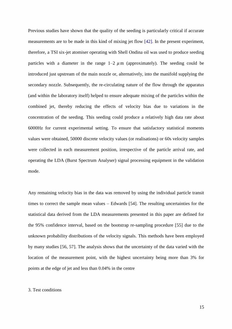
3.1. Primary jet flow

The coordinate system was defined in terms of the axial (x) and vertical (y) directions, taking

the origin of the coordinates to be at the centre-line of the jet in the nozzle exit plane, as

shown in Fig. 2.

Fig. 4. Natural jet – without excitation - variation of the time-averaged axial velocity

component and normalised velocity fluctuations at the centre-line for different

Reynolds numbers.

Fig. 4a compares the decay of the axial velocity component at the centre-line (Ucl/Ue) for

Reynolds numbers of 1.5×104, 2.6×10

4, 5×10

4, 7×10

4 and 1.7×10

5, based upon the diameter

D and the mean velocity Ue in the exit plane of the primary nozzle. It is apparent that the rate

of decay of the axial velocity component along the axis of the jet (the centre-line) reduces

with increasing Reynolds numbers. For example, the centre-line velocity falls below 80% of

the nozzle exit velocity at x/D = 6 for Re = 1.5 ×104. In contrast, at a Reynolds number of

1.7×105, the centre-line velocity at x/D = 6 only falls to 95% of the value at the nozzle exit

plane. Moreover, the axial variations of the axial velocity at the centre-line collapse into a

single curve for Reynolds numbers greater than 5x104. This similarity also appeared in

previous measurements of a natural jet – see, for example, the results of Crow and

Champagne [12] for Reynolds numbers in the range 6.2×104

to 1.24×105.

0 1 2 3 4 5 6 70.75

0.8

0.85

0.9

0.95

1

Ucl

/Ue

(a) x/D

0 1 2 3 4 5 6 70

0.02

0.04

0.06

0.08

0.1

0.12

0.14

0.16

urm

s /U

e

(b) x/D

1.5x104

2.6x104

5x104

7x104

1.7x105

1.5x104

2.6x104

5x104

7x104

1.7x105

17

Fig. 4b compares the distributions of the normalised axial velocity fluctuations (u' /Ue) on the

central axis for the five different Reynolds numbers. It is seen that the normalised

fluctuations increases with the downstream distance in the natural jet. As for the decay of the

centre-line velocity, these distributions show similarity at Reynolds numbers higher than

5×104. Furthermore, for the lower Reynolds numbers (Re = 2.6×10

4 and 1.5×10

4), it can be

seen that the turbulence intensities at the centre-line were about 20 to 60% greater than those

at higher Reynolds numbers in corresponding axial stations.

Due to the similarity of the mean axial velocity distributions observed for Reynolds numbers

Re ≥ 5×104, and for reasons of convenience, only one primary jet velocity was chosen at

which to compare the control effects exerted by the different excitation modes. In these

experiments, therefore, the mean velocity of the primary jet in the nozzle exit plane was set to

7.6 m/s, corresponding to a Reynolds number Re = 5×104. Under these conditions, the

normalised axial velocity fluctuations at the centre-line in the nozzle outlet plane, based on

the axial component of the velocity fluctuations was approximately 1%.

Previous workers have shown that two dominant frequencies are likely to exist in the jet flow

produced by an axisymmetric nozzle. These correspond to the shear-layer and preferred

modes of development [4, 14]. In either situation, the dominant frequency, f, can be

expressed in terms of a Strouhal number, defined by the alternative expressions:

𝑆𝑡𝐷 =𝑓𝐷

𝑈𝑒 (1)

𝑆𝑡𝜃 =𝑓𝜃

𝑈𝑒 (2)

18

Here, f is taken to be the frequency of the excitation, Ue is the jet nozzle exit velocity, D is

the exit diameter of the primary nozzle, and is the momentum thickness of the boundary

layer.

From the literature [4], the shear layer instability corresponds to a Strouhal number St =

0.016. This translates to a frequency of approximately 181 Hz in the present case based on

the momentum thickness = 0.00067 m measured at 1mm away from the exit plane to

estimate. In contrast, the preferred mode can be expected to occur for a Strouhal number StD

= 0.40, which represents a frequency of approximately 32 Hz. This preferred Strouhal

number is higher than 0.3 is because of the large scale of the jet (D/2 =76). The change of

scaling behaviour occurs at D/2 = 120 [4].

3.2. Secondary annular flow

To gain a better understanding of how the different periodic modes can arise in an

aerodynamically excited free jet, LDA was employed to determine the time variations of the

axial velocity component in the secondary annular jet, close to the nozzle exit plane. The

single measurement position (i.e. the crossing point of the four laser beams) was located just

0.5 mm downstream of the nozzle exit plane, at the mid-height of the annulus, and the valve

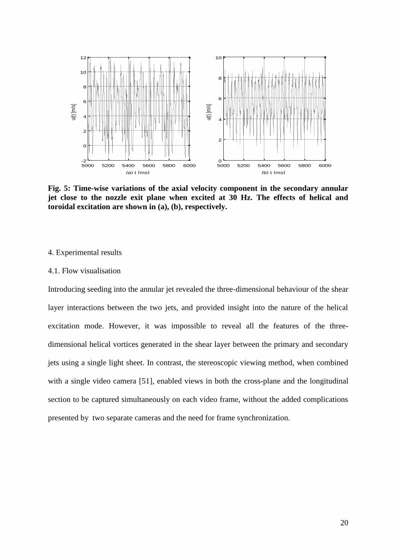
was rotated at 30 revolutions/s. As shown in Fig. 5a, the waveform of the helical excitation

mode at an excitation frequency of 30 Hz reveals very strong amplitude modulation of the

periodic fluctuations. Not unexpectedly, the high frequency component corresponds to a

frequency of six times the rotational frequency of the valve, whereas the modulation

frequency corresponds to the actual rotational speed of the valve. Additionally, negative

values of the axial velocity component can be observed over a part of each pulsation cycle. In

contrast, for the toroidal excitation shown in Fig. 5b, the waveform is clearly sinusoidal, with

19

constant amplitude and a frequency of 30 Hz. There is no evidence of any modulation, or of

any flow reversal.

The secondary volumetric flow rate is non-dimensionalised in terms of the flow rate through

the primary nozzle, and is defined by the expression:

𝑉𝑅 =𝑄𝑆

𝑄𝑃 (3)

where Qs is the time-averaged volumetric flow rate of the pulsed annular flow, and Qp is the

time-averaged volumetric flow rate of the primary jet flow. Consequently, the parameter VR

indicates the strength of the secondary annular flow, relative to the volumetric flow in the

primary jet. Previous studies have shown that only a relatively low secondary flow rate is

required to achieve good control. The secondary flow rate (Qs) was therefore set to

approximately 2% of the primary flow rate (Qp) so that the effectiveness of the two different

aerodynamic excitation modes could be examined.

The systematic studies performed by Szajner, Nixon, Al-Sudane and Zhang [42-46, 51-53]

have confirmed that the development of the free jet can be controlled quite effectively for a

range of volumetric flow ratios (VR) when toroidal excitation is applied at frequencies

corresponding to one of the preferred modes. For the present study, it is worth restating, that

these two frequencies were fairly close. Flow visualisation [51-53] has also confirmed that

the toroidal vortices are strengthened by the excitation at these frequencies, and are

convected downstream without pairing (or merging). A Strouhal number of StD = 0.4 was

therefore chosen for the detailed tests to compare the control effects of the toroidal and

helical excitation modes.

20

Fig. 5: Time-wise variations of the axial velocity component in the secondary annular

jet close to the nozzle exit plane when excited at 30 Hz. The effects of helical and

toroidal excitation are shown in (a), (b), respectively.

4. Experimental results

4.1. Flow visualisation

Introducing seeding into the annular jet revealed the three-dimensional behaviour of the shear

layer interactions between the two jets, and provided insight into the nature of the helical

excitation mode. However, it was impossible to reveal all the features of the three-

dimensional helical vortices generated in the shear layer between the primary and secondary

jets using a single light sheet. In contrast, the stereoscopic viewing method, when combined

with a single video camera [51], enabled views in both the cross-plane and the longitudinal

section to be captured simultaneously on each video frame, without the added complications

presented by two separate cameras and the need for frame synchronization.

5000 5200 5400 5600 5800 6000-2

0

2

4

6

8

10

12

(a) t [ms]

u(t)

[m/s

]

5000 5200 5400 5600 5800 60000

2

4

6

8

10

(b) t [ms]

u(t)

[m/s

]

21

(a) t= 0s

(b) t= 0.04s

(c) t= 0.08s

(d) t= 0.12s

(e) t= 0.16s

(f) t=0.2 s

1

1

2

22

(g)

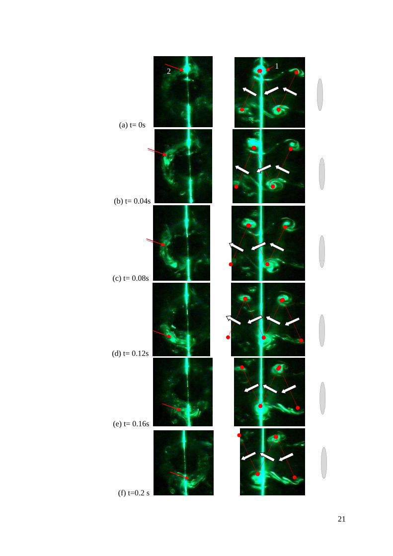
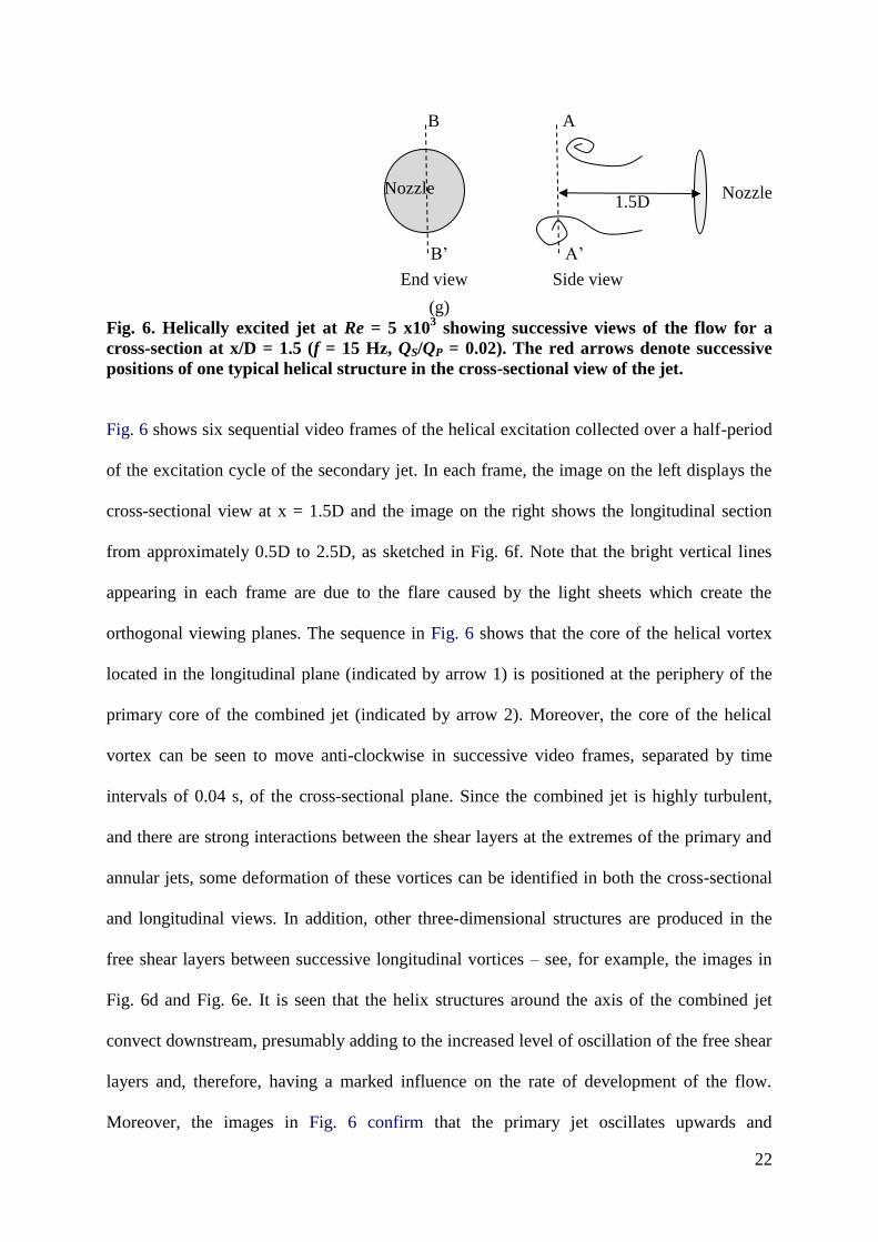
Fig. 6. Helically excited jet at Re = 5 x103 showing successive views of the flow for a

cross-section at x/D = 1.5 (f = 15 Hz, QS/QP = 0.02). The red arrows denote successive

positions of one typical helical structure in the cross-sectional view of the jet.

Fig. 6 shows six sequential video frames of the helical excitation collected over a half-period

of the excitation cycle of the secondary jet. In each frame, the image on the left displays the

cross-sectional view at x = 1.5D and the image on the right shows the longitudinal section

from approximately 0.5D to 2.5D, as sketched in Fig. 6f. Note that the bright vertical lines

appearing in each frame are due to the flare caused by the light sheets which create the

orthogonal viewing planes. The sequence in Fig. 6 shows that the core of the helical vortex

located in the longitudinal plane (indicated by arrow 1) is positioned at the periphery of the

primary core of the combined jet (indicated by arrow 2). Moreover, the core of the helical

vortex can be seen to move anti-clockwise in successive video frames, separated by time

intervals of 0.04 s, of the cross-sectional plane. Since the combined jet is highly turbulent,

and there are strong interactions between the shear layers at the extremes of the primary and

annular jets, some deformation of these vortices can be identified in both the cross-sectional

and longitudinal views. In addition, other three-dimensional structures are produced in the

free shear layers between successive longitudinal vortices – see, for example, the images in

Fig. 6d and Fig. 6e. It is seen that the helix structures around the axis of the combined jet

convect downstream, presumably adding to the increased level of oscillation of the free shear

layers and, therefore, having a marked influence on the rate of development of the flow.

Moreover, the images in Fig. 6 confirm that the primary jet oscillates upwards and

Nozzle

B

B’

End view

Nozzle

A

A’

Side view

1.5D

23

downwards in the vertical longitudinal plane defined by the light sheet, as indicated by the

thick arrows. This suggests that the helical excitation causes the primary jet to deflect away

from the input position of the secondary exciting jet, with the instantaneous offset precessing

around the centre-line of the core flow. In combination, these effects greatly accelerate the

mixing process and cause the jet to expand more rapidly.

4.2. Distributions of the time averaged velocity and turbulent velocity fluctuations

Fig. 7 compares the contours of the axial and radial velocity components and the associated

turbulence intensities for the natural and helically excited jet (with StD = 0.4). It is apparent

that the potential core, corresponding to the region in which the axial velocity is constant and

the normalised velocity fluctuations (u'/Ue) remain less than 0.1, is over five diameters long

for the natural jet. In contrast, when aerodynamic excitation was applied in the helical mode

by means of the relatively weak annular secondary flow (for which QS = 2% QP), the

development of the jet was changed significantly. Then, the potential core was eroded rapidly

by the action of the helical structures in the near-field, and its length was reduced to three

diameters. Furthermore, The peak and trough radial velocities are evident in the top and

bottom shear layers at four diameter downstream – see Fig. 7f. The corresponding peak and

trough radial velocities in the natural jet flow, in contrast, appear between six and eight

diameters downstream, as revealed in Fig 7b. This accelerated development of the combined

jet is clearly the result of the vortical structures producing additional wobbling motion around

the axis of the jet flow in the near field. The rate of spread of the jet is increased by the

helical excitation, and the non-dimensional velocity fluctuations (u'/Ue) rises to more than

0.18 in the mixing layer close to the nozzle exit plane, before reducing rapidly to levels lower

than that in the natural jet beyond eight diameters.

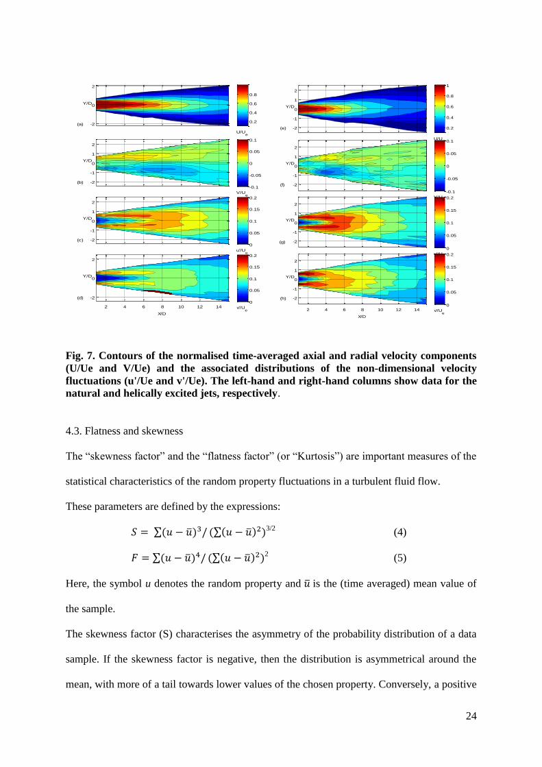
24

Fig. 7. Contours of the normalised time-averaged axial and radial velocity components

(U/Ue and V/Ue) and the associated distributions of the non-dimensional velocity

fluctuations (u'/Ue and v'/Ue). The left-hand and right-hand columns show data for the

natural and helically excited jets, respectively.

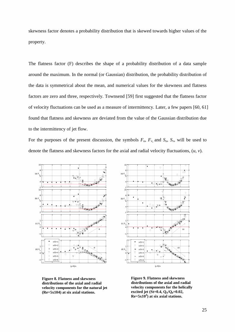
4.3. Flatness and skewness

The “skewness factor” and the “flatness factor” (or “Kurtosis”) are important measures of the

statistical characteristics of the random property fluctuations in a turbulent fluid flow.

These parameters are defined by the expressions:

𝑆 = ∑(𝑢 − �̅�)3/ (∑(𝑢 − �̅�)2)3/2 (4)

𝐹 = ∑(𝑢 − �̅�)4/ (∑(𝑢 − �̅�)2)2 (5)

Here, the symbol u denotes the random property and �̅� is the (time averaged) mean value of

the sample.

The skewness factor (S) characterises the asymmetry of the probability distribution of a data

sample. If the skewness factor is negative, then the distribution is asymmetrical around the

mean, with more of a tail towards lower values of the chosen property. Conversely, a positive

Y/D

(a) -2

0

2

U/Ue

0.2

0.4

0.6

0.8

Y/D

(c) -2

-1

0

1

2

u'/Ue

0

0.05

0.1

0.15

0.2

X/D

Y/D

(d)

2 4 6 8 10 12 14

-2

0

2

v'/Ue

0

0.05

0.1

0.15

0.2

Y/D

(b) -2

-1

0

1

2

V/Ue

-0.1

-0.05

0

0.05

0.1

Y/D

(e) -2

-1

0

1

2

U/Ue

0.2

0.4

0.6

0.8

1

Y/D

(g) -2

-1

0

1

2

u'/Ue

0

0.05

0.1

0.15

0.2

X/D

Y/D

(h)

2 4 6 8 10 12 14

-2

-1

0

1

2

v'/Ue

0

0.05

0.1

0.15

0.2

Y/D

(f) -2

-1

0

1

2

V/Ue

-0.1

-0.05

0

0.05

0.1

25

skewness factor denotes a probability distribution that is skewed towards higher values of the

property.

The flatness factor (F) describes the shape of a probability distribution of a data sample

around the maximum. In the normal (or Gaussian) distribution, the probability distribution of

the data is symmetrical about the mean, and numerical values for the skewness and flatness

factors are zero and three, respectively. Townsend [59] first suggested that the flatness factor

of velocity fluctuations can be used as a measure of intermittency. Later, a few papers [60, 61]

found that flatness and skewness are deviated from the value of the Gaussian distribution due

to the intermittency of jet flow.

For the purposes of the present discussion, the symbols Fu, Fv, and Su, Sv, will be used to

denote the flatness and skewness factors for the axial and radial velocity fluctuations, (u, v).

2

4

6

8

10

(a) Fu

2

4

6

8

10

(b) Fv

-1

0

1

(c) Su

8

-1

0

1

(d) Sv

-8

(y-R)/x

x/D=1

x/D=2

x/D=3

x/D=4

x/D=5

x/D=6

2

4

6

8

10

(a) Fu

2

4

6

8

10

(b) Fv

-1

0

1

(c) Su

10

-1

0

1

(d) Sv

-10

(y-R)/x

x/D=1

x/D=2

x/D=3

x/D=4

x/D=5

x/D=6

Figure 8. Flatness and skewness

distributions of the axial and radial

velocity components for the natural jet

(Re=5x104) at six axial stations.

Figure 9. Flatness and skewness

distributions of the axial and radial

velocity components for the helically

excited jet (St=0.4, QS/Q0=0.02,

Re=5x104) at six axial stations.

26

Figs. 8 and 9 show the measured distributions of these statistical factors for the turbulent

velocity fluctuations in the axial and radial directions in the six downstream locations. Red

lines denotes values of the skewness and flatness factors for normal distribution. For both the

natural and the helically excited jet, the data display excellent self-similarity for successive

downstream stations across the combined jet when plotted in a non-dimensional form. As

might be expected, the experimental data become more scattered towards the inner edges of

the jet for (𝑦−𝑅)

𝑥≤ −0.1 because of the large amplitude, low frequency, velocity fluctuations

which dominate these regions. However, the velocity probability distributions appear to

satisfy the conditions for a normal distribution in the potential core, and in the region close to

the middle of the mixing layer (𝑦−𝑅)

𝑥= 0 . But these two flow regions have absolutely

different flow properties. The flow is stable with small velocity fluctuations in the core flow,

as indicated from fig. 7a and 7e. In contrast, the mixing layer is full of turbulence where the

highest intermittency or the maximum fluid mixing takes place. Therefore, flatness and

skewness can be used as a measure of intermittency in the mixing layer by combine the

velocity fluctuations. The anti-symmetrical distributions of the skewness about the centre-

line of the mixing region indicate the directions in which the turbulent fluctuations transfer

momentum in the radial direction.

Comparing Figs. 8a and 9a, it is evident that the effect of the helical excitation is to reduce

the flatness factor for the axial velocity fluctuations at each radial position, especially within

the mixing layer (|𝑦 − 𝑅| < 0.1). This makes it closer to the Gaussian value (3) which is

related with the maximum flow mixing or the highest intermittency induced by the equal

probability of ejection events from the core of the jet flow and entrainment events from the

ambient flow. Especially for x > 4D, the flatness become the Gaussian value due to the end of

the potential core of the jet flow. Presumably, this also helps to explain some of the

experimental scatter.

27

Moreover, the skewness factors in both cases show a linear variation with the radius across

the mixing layer. The slope of the line is approximately ±8 for the helical excitation (Fig. 7c),

compared with the value of ±10 for the natural jet (Fig. 8c). Furthermore, the linear

relationship extends over a wider range of the radius, for −0.1 <(𝑦−𝑅)

𝑥< 0.2 , compared to

−0.06 <(𝑦−𝑅)

𝑥< 0.1 in the natural jet. These changes can be attributed to the thicker and

more energetic mixing layer produced by the helical excitation. Therefore, flow in the mixing

layer has a higher intermittency and flow mixing at each radial position comparing with the

natural jet.

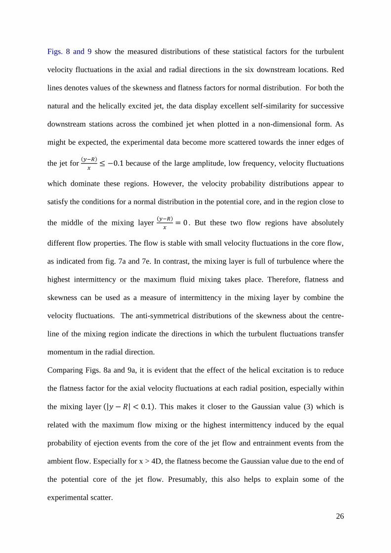
4.4. Energy spectra for the axial velocity fluctuations

Since the LDA technique does not provide uniform (constant time interval) sampling of the

flow velocity component, the ‘Resample and Hold’ technique [58] was used to produce

power spectra from the randomly captured data. Fig. 10 shows the energy spectra for the

axial velocity component on the axis of the combined jet flow at five downstream positions

(in the range x/D = 1 to 5) for both the natural and the excited jets.

10-8

10-6

10-4

10-2

-5/3

-3

(a) f [Hz]

PS

D

X=1D

X=2D

X=3D

X=4D

X=5D

10-8

10-6

10-4

10-2

-5/3

-3

(b) f [Hz]

PS

D

X=1D

X=2D

X=3D

X=4D

X=5D

Figure 10. Comparison of the power spectra on the centre-line of the excited jet

flow: (a) natural jet, (b) helically excited jet (St=0.4).

28

The spectra for the natural jet reveal clear spectral peaks at positions up to five diameters

from the nozzle exit plane, indicating the regular passage of coherent structures in the near

field. For increasing distance downstream, the passing frequency reduces in a systematic way,

and the reduction in the frequency of the spectral peak is a particularly pronounced between

x/D = 1 and 3. In this region, flow visualisation [51–53] has indicated that longitudinal

vorticity is formed and that some merging of the naturally occurring toroidal vortices may

occur. For comparison, Fig. 10b shows the energy spectrum for the helically excited jet in

several axial positions. In this case, there is a fixed peak of 30 Hz at every downstream

position, corresponding to the excitation frequency, and no evidence of any merging of the

vortical structures. Moreover, in the measurement planes at one and two diameters from the

nozzle exit plane, harmonic frequencies of 60Hz and 90 Hz can be observed. These spectral

peaks provide further evidence for the flow interactions occurring in the near field of the jet

during the formation of the helical vortices. Interestingly, similar observations were made in

a helically excited flame by Chao et al. [49].

For the natural jet, once similarity has been established beyond five diameters from the

nozzle exit plane, the spectra obey the anticipated minus five-thirds (-5/3) law in the inertial

sub-range. At higher frequencies, however, dissipation causes faster decay of the natural jet

and the spectra follow the minus three (-3) law. In contrast, for the helically excited jet, there

are obvious increases in the energy of the fluctuations for frequencies between 102 Hz and

103 Hz at three and four diameters downstream.

The energy spectra for the axial turbulent velocity component with the helical excitation are

practically the same at the two downstream positions of x/D = 4 and 5 and both follow the -

5/3 law. Furthermore, the boundary between the two spectral regions (given by the

29

intersection between the lines with slopes of -5/3 and -3) lies at a lower frequency, occurring

at approximately 103 in the excited jet flow, compared with 4x10

3 for the natural jet. This

confirms that the coherent helical structures in the mixing layers enables the inertial sub-

range to extend over a smaller range of frequencies, and that dissipation starts at a lower

frequency (or larger scale). In consequence, mixing of the excited jet is greatly accelerated.

4.5. Jet mixing parameters

Following the practices established when examining the behaviour of a natural jet, three

important parameters based on the time mean velocity distributions can be used. These are

the decay of the axial velocity at the centre-line of the combined jet, the variation of the half-

width, and the rate of entrainment (on the assumption of perfect axial symmetry).

Comparison with equivalent values for the natural jet again enables the effects of the helical

excitation to be quantified.

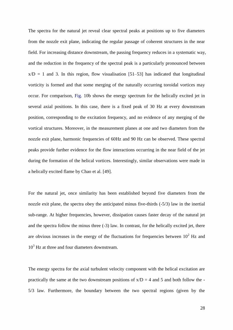
Fig. 11a compares the decay of the centre-line velocity for the jet excited in the helical mode,

with results for the toroidal excitation mode, and the natural jet. It is noted that all these

results were obtained using essentially the same flow apparatus (see Fig. 1), which implies

that a direct comparison is fully justified. When compared with the results for the natural jet,

0 5 10 15

0.4

0.5

0.6

0.7

0.8

0.9

1

Ucl

/Ue

(a) x/D

0 5 10 150.02

0.04

0.06

0.08

0.1

0.12

0.14

0.16

0.18

u rm

s/U

e

(b) x/D

natural jet

toroidal

helical

natural jet

toroidal

helical

Figure 11. Centre-line distributions of the time averaged axial velocity component

and the axial velocity fluctuations as a function of axial position for Re=5x104.

30

the toroidal excitation is seen to produce more rapid decay of the centre-line velocity after

four diameters. However, the helical excitation produces even stronger velocity decay on the

centre-line, starting at three diameters from the exit plane. Moreover, the centre-line velocity

produced by the helical excitation is always lower than for the toroidal excitation, falling to

68% of the nozzle exit velocity at x/D = 6, and 30% at x/D = 15. In comparison, the

corresponding figures for the natural jet and the jet with toroidal excitation are (92%, 42%)

and (88%, 41%), respectively.

Fig. 11b compares the variation of the normalised axial velocity fluctuations (u'/Ue) along the

centre-line for the different excitation modes. For the jet flow with toroidal excitation, the

shape of the distribution of the normalised velocity fluctuations (u'/Ue) shows a small peak

near x/D = 3, and it reaches a maximum at x/D = 7. In contrast, Crow and Champagne [12]

observed several maxima in a natural jet and concluded that the first peak (around x/D = 9)

was caused by the fluctuation of the free shear layer at the periphery of the jet. Examination

of the data for the helical excitation reveals just one peak in the distribution of the centre-line

velocity fluctuations, and this occurs much earlier (at around x/D = 5). Moreover, the peak

intensities for the excited jet are more than 20% higher than for the natural jet, an increase

that may be attributed to the large-scale oscillations of the main jet due to the action of the

helical excitation.

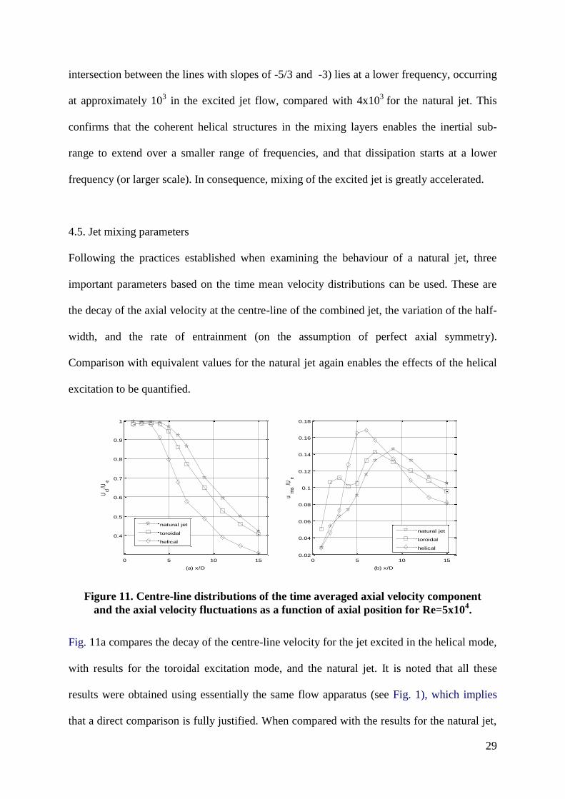
An alternative measure of the rate of development of the excited jet is offered by the half-

radius, R0.5, expressed non-dimensionally in terms of the radius R of the nozzle in the exit

plane. R_0.5 is the radius where the streamwise mean velocity becomes half of the centerline

value at the same axial position. The results presented in Fig. 12 show that the helical

excitation increases the rate of spread in comparison with the other situations. For example,

31

at a distance of x/D = 6, the half-radius of the jet with the helical excitation is twice that with

toroidal excitation. Furthermore, although the differences between the half-radius values for

the three types of excited jet do decrease downstream, the helical excitation consistently

produces a wider jet over the whole range considered, i.e. up to fifteen diameters from the

nozzle exit plane.

Figure 12. Axial variation of the jet half-width, showing the influence of excitation.

Figure 13. Entrainment of the jet flow, with and without excitation.

0 2 4 6 8 10 12 14 161

1.5

2

2.5

3

3.5

R0.

5/R

x/D

natural jet

toroidal

helical

0 2 4 6 8 10 12 14 160

0.5

1

1.5

2

2.5

3

3.5

4

4.5

(Q-Q

0)/Q

0

x/D

natural jet

toroidal

helical0.4

0.24

32

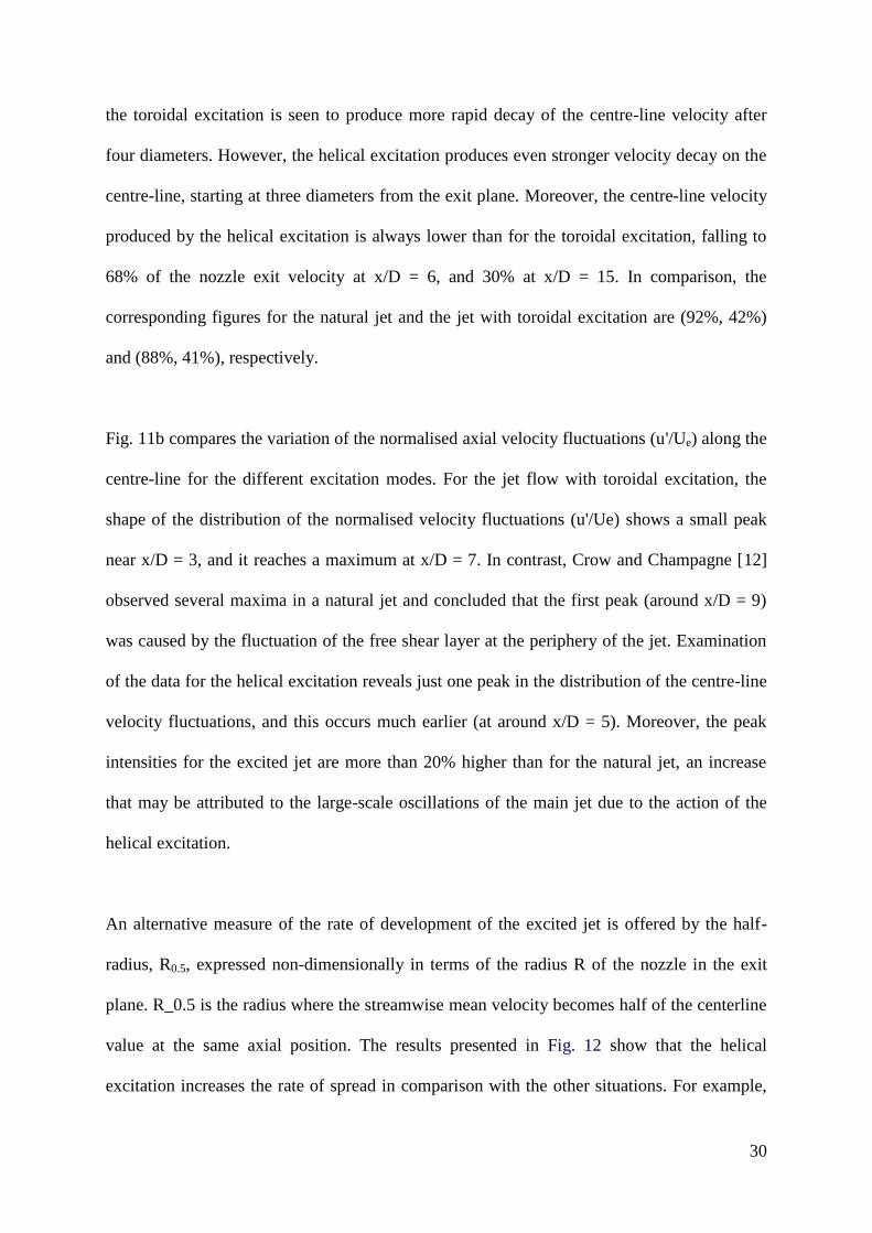
The entrainment rate is another important parameter which can be used to assess the axial

development of the jet under the influence of excitation. In the present study, the total

volumetric flow rate of the jet in each axial position was calculated by integrating the radial

distribution of the time averaged velocity profile between the centre-line and the radius R0.1,

that is to say, the radius at which the axial velocity had fallen to 10% of the centre-line

velocity in that same axial position. To ensure comparability between the values for the

natural and excited jets, the volumetric flow rate Qx for the excited jet at each axial position x

was calculated as a fraction of the total flow rate Q0 through the combined jet in the nozzle

exit plane. This total flow rate Q0 = Qx + QS was then used to normalise the entrainment flow

rate of the measured velocity distributions, assuming axial symmetry. These normalised

results, which correspond directly to the standard definition of the entrainment rate,

𝑑(𝑄−𝑄0)/𝑄0

𝑑𝑥/𝐷, are presented in Fig. 13. It is clear that the data for the natural jet flow show a

well-defined linear increase in volumetric flow rate with a gradient of 𝑑(𝑄−𝑄0)/𝑄0

𝑑𝑥/𝐷= 0.24. In

comparison, the entrainment rate with helical excitation is about 0.4 in the near field (x/D < 4)

although, further downstream, the gradient is reduced. The entrainment rates of both the

helical and toroidally excited jets remain higher than that for the natural jet over the whole

range in which measurements were obtained. These entrainment rates are comparable with

the values found by previous researchers [12, 42].

5. Discussion and Conclusion

An experimental investigation has been described in which aerodynamic excitation has been

used to influence the development of a turbulent free jet. The paper discusses a novel nozzle

arrangement that enables the aerodynamic excitation to be applied to the jet in the helical

mode. It is found that the helical excitation leads to a rate of development in the axial

33

direction which is significantly greater than could be achieved with the toroidal excitation

discussed in previous papers [42-46, 51-53].

The behaviour of the jet has been visualised using a laser light sheet and stereoscopic flow

imaging, supplemented by detailed measurement using two-component laser Doppler

anemometry. These experiments have yielded information on the interactions between the

vortical flow structures generated by the excitation, and the mean flow and turbulence

distributions in the developing jet. Coupling the qualitative results of the visualisation with

the quantitative data derived from the LDA measurements has provided several useful

methods by which the effectiveness of the toroidal and helical forms of excitation can be

compared.

Examination of the energy spectra for the excited jet shows that the helical excitation tends to

concentrate the energy of the turbulence into a narrow band of frequencies centred on the

excitation frequency and reduces the frequency range of the inertial sub-range. In contrast,

the spectra for the natural jet reveal energy peaks that move progressively towards lower

frequencies with increasing distance downstream. These differences in behaviour are a

consequence of the interactions between neighbouring vortical structures, as revealed by the

flow visualisation.

It is concluded that self-similarity of the helically excited jet was achieved after only three

diameters. Moreover, the length of the potential core was reduced to three diameters with

helical excitation, compared with lengths of four diameters for the toroidal excitation and five

diameters for the natural jet. Thus, the aerodynamic excitation is again shown to have a

34

controlling influence on the development of the turbulent jet, and these effects become

especially strong when the excitation is introduced in the helical mode.

References

[1]. A. Michalke, A note on spatially growing three-dimensional disturbances in a free shear

layer. Journal of Fluid Mechanics 38.04 (1969): 765-767.

[2]. A. Michalke, On the instability of the turbulent jet boundary layer. NASA STI/Recon

Technical Report N. 1974 Jun;75.

[3]. G. L. Brown, and A. Roshko. On density effects and large structure in turbulent mixing

layers. Journal of Fluid Mechanics 64.04 (1974): 775-816.

[4]. C.M. Ho and P. Huerre, Perturbed free shear layers. Annual Review of Fluid Mechanics.

1984 Jan;16(1):365-422.

[5]. C.D. Winant, and F.K. Browand, Vortex pairing: the mechanism of turbulent mixing-

layer growth at moderate Reynolds number. Journal of Fluid Mechanics. 1974 Apr

3;63(02):237-55.

[6]. C.M. Ho, L.S. Huang, Subharmonics and vortex merging in mixing layers. Journal of

Fluid Mechanics. 1982 Jun 1;119:443-73.

[7]. M. Samimy, J.-H. Kim, J. Kastner, I. Adamovich, Y. Utkin, Active control of high-speed

and high-Reynolds-number jets using plasma actuators, J Fluid Mech, 578, (2007), 305-

330.

[8]. E.J. Gutmark, K.C. Schadow, K.H. Yu, Mixing enhancement in supersonic free shear

flows. Annual Review of Fluid Mechanics. 1995 Jan;27(1):375-417.

[9]. E. Gutmark, C.M. Ho, Preferred modes and the spreading rates of jets. Physics of Fluids

(1958-1988). 1983 Oct 1;26(10):2932-8.

35

[10]. R. D. Blevins, Formulas for natural frequency and mode shape, Van Nostrand

Reinhold. (1979).

[11]. T.C. Corke, S.M. Kusek, Resonance in axisymmetric jets with controlled helical-

mode input. Journal of Fluid Mechanics. 1993 Apr 1;249:307-36.

[12]. S.C. Crow, F.H. Champagne, Orderly structure in jet turbulence. J. Fluid Mech. 1971

Aug 16;48(3):547-91.

[13]. K.B. Zaman, A.K. Hussain, Vortex pairing in a circular jet under controlled excitation.

Part 1. General jet response. Journal of fluid mechanics. 1980 Dec 11;101(03):449-91.

[14]. A.F. Hussain, K.B. Zaman, The ‘preferred mode’of the axisymmetric jet. Journal of

Fluid Mechanics. 1981 Sep 1;110:39-71.

[15]. W.C. Reynolds, E.E. Bouchard, The effect of forcing on the mixing-layer region of a

round jet. InUnsteady Turbulent Shear Flows 1981 (pp. 402-411). Springer Berlin

Heidelberg.

[16]. D.G. Crighton, M.Gaster, Stability of slowly diverging jet flow. Journal of Fluid

Mechanics. 1976 Sep 24;77(02):397-413.

[17]. P. Plaschko, Helical instabilities of slowly divergent jets. Journal of Fluid Mechanics.

1979 May 28;92(02):209-15.

[18]. J. Cohen, I. Wygnanski, The evolution of instabilities in the axisymmetric jet. Part 1.

The linear growth of disturbances near the nozzle. Journal of Fluid Mechanics. 1987 Mar

1;176:191-219.

[19]. T.C. Corke, F. Shakib, H.M. Nagib, Mode selection and resonant phase locking in

unstable axisymmetric jets. Journal of Fluid Mechanics. 1991 Feb 1;223:253-311.

[20]. A. Michalke, Instability of compressible circular free jet with consideration of the

influence of the jet boundary layer thickness. NASA TM 75190. (1977).

36

[21]. H. Hu, W. Shousheng, S. Gongxin, and E. L. Yagoda, Effect of tabs on the vortical

and turbulent structures of jet flows. Vol. 237, ASME, New York, NY, USA, San Diego,

CA, USA, (1996), 77-84.

[22]. M.F. Reeder, M. Samimy, The evolution of a jet with vortex-generating tabs: real-

time visualization and quantitative measurements. Journal of Fluid Mechanics. 1996 Mar

25;311:73-118.

[23]. M.J. Carletti, C.B. Rogers, D.E. Parekh. Parametric study of jet mixing enhancement

by vortex generators, tabs, and deflector plates. ASME-PUBLICATIONS-FED.

1996;237:303-12.

[24]. C.J. Bourdon, J.C. Dutton. Visualizations and measurements of axisymmetric base

flows altered by surface disturbances. AIAA paper. 2001;286:2001.

[25]. K.B. Zaman, J. Bridges, D. Huff, Evolution from ‘tabs’ to ‘chevron technology’-a

review. International Journal of Aeroacoustics. 2011 Sep 28;10(5-6):685-710.

[26]. E.J. Gutmark, F.F. Grinstein, Flow control with noncircular jets 1. Annual review of

fluid mechanics. 1999 Jan;31(1):239-72.

[27]. M. Samimy, K. B. M. Q. Zaman, M. F. Reeder, Effect of tabs on the flow and noise

field of an axisymmetric jet. AIAA J. 31, (1993),609.

[28]. K. B. Zaman, M. F. Reeder, and M. Samimy, Control of an axisymmetric jet using

vortex generators. Phys. Fluids 6, (1994)778–793

[29]. K.B. Zaman, Spreading characteristics of compressible jets from nozzles of various

geometries. Journal of Fluid Mechanics. 1999 Mar 25;383:197-228.

[30]. V. Mengle, Optimization of lobe mixer geometry and nozzle length for minimum jet

noise. In6th Aeroacoustics Conference and Exhibit 2000 Jun (p. 1963).

37

[31]. H. Hu, T. Saga, T. Kobayashi, and N. Taniguchi, A study on a lobed jet mixing flow

by using stereoscopic particle image velocimetry technique. Physics of Fluids, Vol. 13,

No. 11, (2001), 3425-3441

[32]. D. E. Nikitopoulos, J. W. Bitting, and S. Gogineni, Comparisons of initially turbulent,

low-velocity-ratio circular and square coaxial jets, AIAA Journal, Vol. 41, No. 2, (2003),

230-239

[33]. N. H. Saiyed, K. L. Mikkelsen, J. E. Bridges, Acoustics and thrust of quiet separate

flow high-bypass-ratio nozzles, AIAA J, 38, (2003),1166- 1172

[34]. B. Callender, E. Gutmark, S. Martens, Far-field acoustic investigation into chevron

nozzle mechanisms and trends, AIAA J, 43, (2005), 87-95

[35]. J.U. Schlüter, Static control of combustion oscillations by co-axial flows: a Large

Eddy Simulation investigation. AIAA J. Propuls. Power 20, (2004), 460-467

[36]. D. Papamoschou, Fan Flow Deflection in Simulated Turbofan Exhaust, AIAA Journal,

Vol. 44, No.12, (2006), 3088-3097

[37]. B. Henderson, K. Kinzie, J. Whitmire, & A. Abeysinghe, The impact of fluidic

chevrons on jet noise. AIAA Paper 2005-2888

[38]. V. H. Arakeri, A. Krothapalli, V. Siddavaram, M. B. Alkislar, & L.M. Lourenco, On

the use of microjets to suppress turbulence in a Mach 0.9 axisymmetric jet. J. Fluid Mech.

490,( 2003), 75–98

[39]. A. Krothapali, L. Venkatakrishnan, L. Lourenco, B. Greska, & R. Elavarasan,

Turbulence and noise suppression of a high-speed jet by water injection. J. Fluid Mech.

491,( 2003), 131–159

[40]. M. Konig, A. V. G. Cavalieri, P. Jordan, Y. Gervais, Jet-noise control by fluidic

injection from a rotating plug: linear and non-linear sound source mechanisms, 19th

AIAA/CEAS Aero-acoustics Conference, AIAA Paper 2013-2145, ( 2013)

38

[41]. M. K. Ibrahim, R. Kunimura, Y. Nakamura, Mixing enhancement of compressible

jets by using unsteady micro-jets as actuators, AIAA Journal 40, 4, (2002), 681–688.

[42]. A. Szajner, J.T. Turner, Visualisation of an aerodynamically excited free jet, Proc. Int.

Conf. Flow Visualisation, Paris, (4), (1986), 533–539.

[43]. A. Szajner, J.T. Turner, Controlled development of a turbulent free jet, Proc. 2nd Int.

Symposium on Fluid Control, Measurement, Mechanics and Flow Visualisation

(FLUCOME ’88), Sheffield, UK, (1988), 406–412.

[44]. P.L. Nixon, J.T. Turner, Use of pulsed LS and PIV to study an aerodynamically

excited free jet, Proc. 7th EALA Conf. on Laser Anemometry, Karlsruhe, 1997, 543–549,

ISBN 3-9805613-0-5.

[45]. A.H.S. Al-Sudane, Experimental study of the development of a turbulent free jet, with

and without aerodynamic excitation, PhD Thesis, University of Manchester, 1996.

[46]. A.H.S. Al-Sudane, J.T. Turner, LDA measurements in an excited turbulent jet, Proc.

7th EALA Conference on Laser Anemometry, Karlsruhe (1997), 535–535. ISBN 3-

9805613-0-5.

[47]. N.H. Saiyed, K.L. Mikkelsen, J.E. Bridges. Acoustics and thrust of quiet separate-

flow high-bypass-ratio nozzles. AIAA journal. 2003 Mar;41(3):372-8.

[48]. W.C. Reynolds, D.E. Parekh, P.J.D. Juvet, M.J.D. Lee, Bifurcating and blooming jets,

Annual Review Fluid Mechanics 35, (2003), 295–315.

[49]. Y.-C. Chao, Y.-C. Jong, H.-W. Sheu, Helical-mode excitation of lifted flames using

piezoelectric actuators, Experiments in Fluids 28, (2000), 11–20.

[50]. C.R. Koch, M.G. Mungal, W.C. Reynolds, J.D. Powell, Helical mode in an

acoustically excited round air jet, Physics of Fluids A 1, (1989), 1443 (9)

[51]. S. Zhang, J.T. Turner, Visualisation of the large-scale structures in an

aerodynamically excited turbulent jet, Measurement Science and Technology 21, (2010).

39

[52]. S. Zhang, K. Bremhorst, J.T. Turner, Stereoscopic visualisation of the large-scale

structures in an aerodynamically excited turbulent jet, Proc. 7th Int. Symposium on Fluid

Control, Measurement and Flow Visualization (FLUCOME), Sorrento, Italy, (2003).

[53]. S. Zhang, Optical diagnostics and digital imaging applied to natural and

aerodynamically excited turbulent jets, PhD Thesis, The University of Manchester,

(2006).

[54]. R.V. Edwards, Report of the A.S.M.E. Special Panel on “Statistical particle bias in

laser anemometry”, J. Fluids Engineering, 109, (1987), 89-93.

[55]. B. Efron, 1982: The jackknife, the bootstrap, and other resampling plans. pp. 27–36.

CBM-NSF Regional Conference Series in Applied Mathematics 38, Society for

Industrial and Applied Mathematics, Philadelphia.

[56]. D.B. DeGraaff, J.K. Eaton, A high resolution laser Doppler anemometer: design,

qualification, and uncertainty. Exp Fluids20: (2001) 522–530

[57]. P.L. Johnson, R.S. Barlow, Effect of measuring volume length on two-component

laser velocimeter measurements in a turbulent boundary layer. Exp Fluids 8,(1990):137–

144

[58]. H. Nobach, A global concept of autocorrelation and power spectral density estimation

from LDA data sets, 10th International Symposium on Applications of Laser Techniques

to Fluid Mechanics, Lisbon, (2000).

[59]. A.A.Townsend(1956) The Structure of Turbulent Shear Flow. Cambridge University

Press

[60]. I. Wygnanski and H. Fiedler, Some measurements in the self-preserving jet. J. Fluid

Mech. 38, (1969), 577.

40

[61]. R. A Antonia, A. Prabhu, S. E. Stephenson, Conditionally sampled measurements in a

heated turbulent jet. J. Fluid Mech. 72, (1975). 455-80

Nomenclature

D diameter of primary nozzle in the outlet plane

f frequency of pulsation

F flatness factor, dimensionless and defined by equation 5

h annulus height of secondary concentric annular nozzle

QS volumetric flow rate of the secondary jet

QP volumetric flow rate of the primary jet

Q0 total volumetric flow rate of the jet (Qp+Qs)

Qx volumetric flow rate of the jet at axial location x

R radius of primary nozzle in the outlet plane

Re Reynolds number, dimensionless

St Strouhal number, dimensionless and defined by equations 2 and 3

S skewness factor, dimensionless– defined by equation 4

t time period of excitation

u’ root mean square velocity fluctuation in the axial direction

U time averaged axial velocity

Ue time-averaged axial velocity in the nozzle exit plane

v’ root mean square velocity fluctuation in the radial direction

V radial velocity component, m/s

x axial coordinate

y radial coordinate

momentum thickness of the boundary layer