On the Direction of Innovation

Hugo HopenhaynUniversity of California

at Los Angeles∗

Francesco SquintaniUniversity of Warwick†

October 20, 2017

Abstract

How are resources allocated across different R&D areas? We showthat under a plausible set of assumptions, the competitive market al-locates excessive innovative efforts into high returns areas, meaningthose with higher private (and social) payoffs. The underlying sourceof market failure is the absence of property rights on problems to besolved, which are the source of R&D value. The competitive biastowards high return areas comes three distortions: 1) The cannibal-ization of returns of competing innovators; 2) excessive turnover andduplication costs; 3) excessive entry into high return areas results asthe market does not take into account the future value of an unsolvedproblem while a social planner does. Allocation of resources to prob-lem solving leads to a stationary distribution over open problems. Thedistribution of the socially optimal solution stochastically dominatesthat of the competitive equilibrium. A severe form of rent dissipationoccurs in the latter, where the total value of R&D activity equals thevalue of allocating all resources to the least valuable problem solved.

∗Economics Department, UCLA, Bunche Hall 9353, UCLA Box 951477, Los Angeles,CA 90095-1477, USA.†Economics Department, University of Warwick, Coventry CV4 7L, United Kingdom

1

1 Introduction

Innovation resources are quite unequally distributed across different research

areas. This is true not only in the case of commercial innovations but even

so in our own fields of research. Some areas become more fashionable (hot)

than others and attract more attention. A quick look at the distribution

of patenting by different classes since the 80’s reveals significant changes in

the distribution of patent applications: while early on the leading sector was

the chemical industry followed closely by others, starting 1995 the areas of

computing and electronics surpassed by an order of magnitude all other areas

in patent filings. The so-called dot-com bubble is an example of what many

considered excessive concentration in the related field of internet startups.

This example suggests that innovation resources might be misallocated across

different areas and perhaps too concentrated on some, yet to date almost no

economic theory has been devoted to this question.

This shift in innovative activity is likely the result of technological, de-

mographic and other changes that introduce new sets of opportunities and

problems to solve. As new opportunities arise, firms compete by allocating

innovation resources across these opportunities, solving new open problems

and thus creating value. The process continues as new opportunities and

problems arise over time and innovation resources get reallocated. We model

this process and characterize the competitive equilibrium as well as the so-

cially optimal allocations. Our main finding is that the market engages dis-

proportionately in hot R&D lines, characterized by higher expected rates of

return per unit of research input and there excessive turnover of researchers.

1

We model this process as follows. At any point in time there is a set

of open problems (research opportunities) that upon being solved generate

some social and private value v. This value is known at the time research

inputs are allocated and is the main source of heterogeneity in the model.

The research side of the economy is as follows. There is a fixed endowment

-inelastically supplied- of a research input to be allocated across problems,

that for simplicity we call researchers. The innovation technology specifies

probabilities of discovery (i.e. problem solution) as a function of the number

of researchers involved. Ex-ante the expected value of solving a problem is

split equally among the researchers engaged, consistently with a winner-take-

all, as in patent races, or an equal sharing rule. Once a problem is solved,

the researchers involved are reallocated to other problems after paying an

entry cost. We consider both, an environment where the set of problems is

fixed as well as a steady state with exogenous arrival of new problems. Firms

compete by allocating researchers to the alternative research opportunities

to maximize the value per unit input. As there is a large number of firms,

we can equally assume that each researcher maximizes its value by choosing

research lines. As a result, the value of joining any active research line is

equalized.

The key source driving market inefficiency is differential rent dissipation

resulting from competitive entry into research. This is due to the pecuniary

externality imposed by a marginal entrant to all others involved in this re-

search line. It is useful to contrast our results to the standard models of

patent races, where there is a perfectly elastic supply to enter at a cost a

patent race, where competitive forces drive average value down to the entry

2

cost. With a concave discovery function, this exceeds the marginal value of

an entrant, thus resulting in excessive entry. The gap between average and

marginal value is a reflection that part of the return to an entrant comes

from a decrease in the expected returns of the remaining participants, the

pecuniary externality.

In contrast, in our model we assume that the total research endowment

to be allocated is inelastically supplied and entry costs are the same across

all research lines, so there cannot be excessive entry overall. But as we find,

there will be excessive entry in some areas and too little in others, as well

as excessive turnover. It is useful to divide the sources of this misallocation

between static and dynamic ones.

The static source of misallocation arises as the pecuniary externality

changes with the number of researchers in a research line. To illustrate this,

consider the case where the probability of innovation is linear up to a certain

number of researchers m and constant thereafter and there are two research

lines, a ’hot’ one with high value and one with low value. Furthermore,

suppose that given the total endowment of researchers, more than m enter

into the former while less than m in the latter one, so the average values are

equalized. It follows immediately that there is excessive entry into the hot

area, where there are negative pecuniary externalities, and too little in the

low value one, where there are none.

This example suggests that the extent of pecuniary externalities can

vary with scale, and will do so in general. As total discovery probability

is bounded, the effect described in the example will occur in some region

3

and as a result there will be excessive entry into the higher value areas. As

we show in the paper, the distortion holds globally (there is excessive en-

try above a value threshold and too little below) for the canonical model of

innovation considered in the literature.

We now turn to the dynamic sources of misallocation that can be or-

ders of magnitude more important as illustrated by our back-of-the-envelope

calculations. The first one arises from the cost of reallocation. When a re-

searcher joins a research line and succeeds, this generates a capital loss to the

remaining researchers that must incur a new entry cost in order to switch to

a new, equally valuable, research line. This externality grows with the num-

ber of researchers affected and thus with the value v of innovation, leading

to excessive entry into hot areas. The second source is more subtle. As a

consequence of rent dissipation the value of entering any innovation line is

equalized in the competitive equilibrium. In the eyes of competitors, there

is no distinction between different open problems in the future, as they all

give the same value. In contrast, a planner recognizes that better problems

(those with higher v) have higher residual value an so carry a higher future

option value if they are not immediately solved. As a result, the planner is

less rushed to solve these high value problems.

We analyze a steady state allocation with an exogenous arrival of new

problems and endogenous exit of existing ones, resulting from the allocation

of researchers. These two forces determine a stationary distribution for open

problems. High value problems are solved faster in the competitive equi-

librium, due to the biases indicated above, so the corresponding stationary

4

distribution has a lower fraction of good open problems. In addition, as

the distribution of innovators is more skewed than in the optimal allocation,

turnover is higher and so are reallocation costs. This leads to a severe form

of rent dissipation, where in a competitive equilibrium the total value of

R&D activity equals the value of allocating all resources to the least valuable

problem solved. The magnitude of this distortion can be extremely severe,

leading to very large welfare effects as shown by our simple calculations.

Throughout our analysis we assume that the private and social value of

innovations is the same across research lines, or likewise that the ratio of

private to total value is identical. We do this to abstract from some other

important but more obvious sources of misallocation. As patents attempt to

align private incentives with social value, they are of no use in solving the

distortions that we consider. The source of market failure in our model is

the absence of property rights on problems to be solved, which are the source

of R&D value. Patents and intellectual property are no direct solutions to

this problem as they entitle innovators to value once problems have been

solved. Our research suggests that there might be an important role for the

allocation of property rights at an earlier stage.

The paper is organized as follows. The related literature is discussed in

the next section. Section 3 provides a simple example to illustrate the main

ideas in the paper. Section 4 Describe the model and analyzes the static

forces of misallocation. Section 5 considers the reallocation of researchers

and the dynamic sources of misallocation for a fixed set of problems. Section

6 considers the steady state with continuous arrival of new problems. Section

5

7 concludes.

2 Literature Review

We begin the literature review by clarifying how the market inefficiency we

identify is distinct from the forms of market failure previously singled out in

the R&D literature.

Early literature (e.g., Schumpeter, 1911; Arrow, 1962; and Nelson, 1959)

pointed at limited appropriability of the innovations’ social value by inno-

vators, and at limited access to finances as the main distorting forces in

R&D markets, both leading to the implication that market investment in

R&D is insufficient relative to first best.1 A large academic literature has

developed to provide policy remedies, often advocating strong innovation

protection rights,2 and the subsidization of R&D. Wright (1983) compares

patents, prizes, and procurement as three alternative mechanisms to fund

R&D. Patents provide incentives so that they exert R&D effort efficiently,

as they delegate R&D investment decisions to innovators, i.e. to the ‘in-

formed parties,’ but they burden the market with the IP monopoly welfare

loss. Kremer (1998) suggests an ingenious mechanism based on the idea of

1There appears to be significant empirical evidence for these forces. Since the classicalwork of Mansfield et al. (1977) estimates of the social return of innovations calculatethat they may be twice as large as private returns to innovators; whereas evidence of a“funding gap” for investment innovation has been documented, for example, by Hall andLerner (2010), especially in countries where public equity markets for ‘venture capitalistexit’ are not highly developed.

2However, others also underline the negative effects of patents on social welfare throughmonopoly pricing, and on the incentives for future innovations; and Boldrin and Levine(2008) have even provocatively challenged the views that patents are needed to remunerateR&D activity.

6

patent buyout, to design a prize system that provide efficient R&D invest-

ment incentives. Cornelli and Schankerman (1999) show that optimality can

be achieved using either an up-front menu of patent lengths and fees or a

renewal fee scheme. Hopenhayn and Mitchell (2001) show that if innovations

differ both in terms of expected returns and in the likelihood to be replaced

by follow-on invention, then the optimal contract involves a menu of patent

lengths and breadths.

Another known source of market inefficiency is caused by the sequential,

cumulative nature of innovations. This ‘sequential spillover’ problem arises

when, without a ‘first’ innovation, the idea for ‘follow-on’ innovations cannot

exist, and the follow-on innovators are distinct from the first innovator (see

Horstmann, MacDonald and Slivinski, 1985, and Scotchmer, 1991).3 Sum-

marizing the conclusion of the literature that studies optimal patent length

and breadth for this ‘cumulative innovation case’ (e.g., Green and Scotchmer,

1995, Scotchmer, 1996, O’Donoghue et al., 1998, O’Donoghue, 1998, Deni-

colo, 2000), there appears to be a strong argument for protection from literal

imitation (large lagging breadth) if licensing is fully flexible and efficient, and

a general strong argument for leading breadth, whereas strong patentability

requirements receive some support when licensing does not function well. In

terms of mechanism design, Hopenhayn et al. (2006) study a quality ladder

model of cumulative innovations and find the optimal mechanism to be a

mandatory buyout system.

3As well as distorting investment decisions, sequential innovations can also make thetiming of innovation disclosure inefficient (see, for example, Matutes et al., 1996, andHopenhayn and Squintani, 2016).

7

The issue of innovation spillovers may complicate policy design not only

among sequential innovations, but because of ‘horizontal’ market value com-

plementarities or substitutabilities among innovations (see Cardon and Sasaki,

1998, and Lemley and Shapiro, 2007, for example). This possibility is dis-

tinct from the market inefficiency we identify in this paper: our results

hold also in the case of innovations whose market values are independent

of each other. A possible policy remedy to inefficiencies caused by horizontal

spillovers are patent pools: agreements among patent owners to license a set

of their patents to one another or to third parties. Lerner and Tirole (2004)

build a tractable model of a patent pool, and identify a simple condition to

establish whether patent pools are welfare enhancing.4

A recent paper, Bryan and Lemus (2016), provides a valuable general

framework on the direction of innovation that encompasses the models cited

here, as well as models of horizontal spillovers and of sequential innovation.

Building on the interaction across these different kinds of spillovers, they use

their framework to assess when it is optimal to achieve incremental innova-

tions versus large step innovations, and show that granting strong IP rights

to ‘pioneer patents’ may lead to distortions in the direction of R&D. They

also identify market distortions that are entirely independent of the market

inefficiency identified here.5 Relatedly, Acemoglu, Akcigit and Kerr (2016)

4Even further distantly related to our work, there is also a literature studying the wel-fare effects of complementarities and substitutabilities among different research approachesto achieve the same innovation (e.g., Bhattacharya and Mookherjee, 1986; Dasgupta andMaskin, 1987). Of course, this is very different from the analysis of this paper, whichconsiders several innovations, without distinguishing different approaches to achieve anyof them.

5These distortions are demonstrated in a model with costless switching of researchersacross R&D lines, and without duplication of efforts in R&D races, so that it is optimal

8

compute a map of the U.S. innovation network using on 1.8 million U.S.

patents and their citations.

Finally, it is interesting to note that our static misallocation force can be

related to the study of the so-called ‘price of anarchy’ in the congestion games

developed by Rosenthal (1973). These games model a traffic net, in which

drivers can take different routes to reach a destination, and routes get easily

congested. In the optimal outcome, the drivers coordinate in taking different

routes, whereas in equilibrium they excessively take routes that would be

faster if they were not congested by their suboptimal driving choices. The

analysis of our extended model in section 4 identifies economic features of

R&D competition that lead to the ‘congestion’ of hot R&D lines. That these

features (costly switching of R&D resources across R&D lines and duplication

of efforts in R&D lines) lead to congestion is a novel result for the literature

on congestion games, and it may be used as an additional motivation for the

study these games.

to concentrate all R&D resources on a single, most valuable, R&D line, to then move onto the second most valuable one, after the first innovation is discovered, and so on and soforth. Under these assumptions, this paper’s market inefficiency that innovators overinvestin the most valuable R&D line can not arise. Conversely, the distortions identifies in theirpaper do not occur in the simple model of section ?? in which we demonstrate our marketdistortion in its simplest form.

9

3 A simple example

There are two problems with private and social values zH > zL6, and 2

researchers to be allocated to finding their solution. In any of the problems,

the probability of success with one researcher is p and with two is q > p.

We assume that q − p < p, capturing the idea that there is congestion or

superfluous duplication of efforts. This holds in case of independence, where

q = 2p− p2 < 2p. We examine optimal and competitive allocations with one

and two periods.

3.1 One Period Case

Consider first the optimal allocation. Both researchers are allocated to H iff

qzH ≥ p (zL + zH) or likewise:

(q − p) zH ≥ pzL, (1)

with a straightforward interpretation.

For the competitive case, we assume that if two researchers are allocated

toH, then expected payoffs for each are 12qzH . This would happen for instance

in a patent race where all value accrues to the first to solve the problem.

The necessary and sufficient condition for both researchers to work on the H

problem is that1

2qzH ≥ pzL. (2)

6Likewise, we can assume that private values are an equal proportion of social values.Differences in the degree of appropriability are a a very relevant, yet well know source ofinefficiency.

10

It is easy to verify that condition (1) implies (2) so the competitive allocation

will always assign both researchers to H when it is optimal, but might do

so also when it is not. The difference between these two conditions can be

related to the pecuniary externality (market stealing effect) caused by entry

into the H problem that equals (p− q/2) zH . Note that here the externality

is not present when entering into the L problem, since there will be at most

one researcher there. In the more general setting that we examine below

with multiple research inputs, this externality will occur for more than one

research line and its relative strength is a key factor in determining the nature

of the bias in the competitive allocation.

Another interpretation of this external effect is value burning. In the more

general setup with many researchers that we examine below, the expected

value of solving different research problems is equalized to the least attractive

active one. All differential rents from solving more attractive problems are

dissipated.

3.2 Two Period Case

As above, in each period researchers can be allocated to the unsolved prob-

lems. In case both succeed in the first period, then there are no more prob-

lems to solve. If one problem is solved in the first period, then in the optimal

as well as in the competitive allocation both researchers are assigned to solve

the remaining one.

To compare both alternatives, it is convenient to decompose total payoffs

of the alternative strategies into first and second period payoffs. The second

11

period problem is a static one. If only one problem is left, then the two

researchers will be assigned to it. If the two problems remain to be solved,

we will assume for simplicity that condition (1) holds, so that both researchers

are assigned to the H problem. Denoting by wit the total expected payoffs

for each strategy iε {1, 2} in each period tε {1, 2} we can write

w21 = qzH , w22 = q [(1− q) zH + qzL]

w11 = p (zH + zL) , w12 = q[(1− p) zH + pzL − p2zL

]The difference in first period payoffs is identical to the calculation in the

static case. Consider now second period payoffs. The terms in brackets

represent the expected value of the problems that remain to be solved. We

call this the option value effect: as the planner has the option of solving

problems in the second period it recognizes that if not solved in the first

there is a residual value. This is higher when the problem that remains to

be solved is H. Ignoring the quadratic term (which becomes irrelevant in the

continuous time Poisson specification that follows) w12 > w22, so incentives

for allocating initially both researchers to H will be weaker than in the static

case.

Consider now the competitive allocation. Assuming one player chooses

H and letting v2t represent expected payoffs in period t for the other player

when also choosing H and v1t when choosing L, it follows that

v21 =1

2qzH , v22 =

1

2q [(1− q) zH + qzL] =

1

2w22

v11 = pzL, w12 = q[(1− p) zH + pzL − p2zL

]=

1

2w12.

Again we are assuming here that in the second period if both problems

12

remain, the two players will choose H. The difference v21 − v11 is identical

to the one for the one period allocation. As shown above and ignoring the

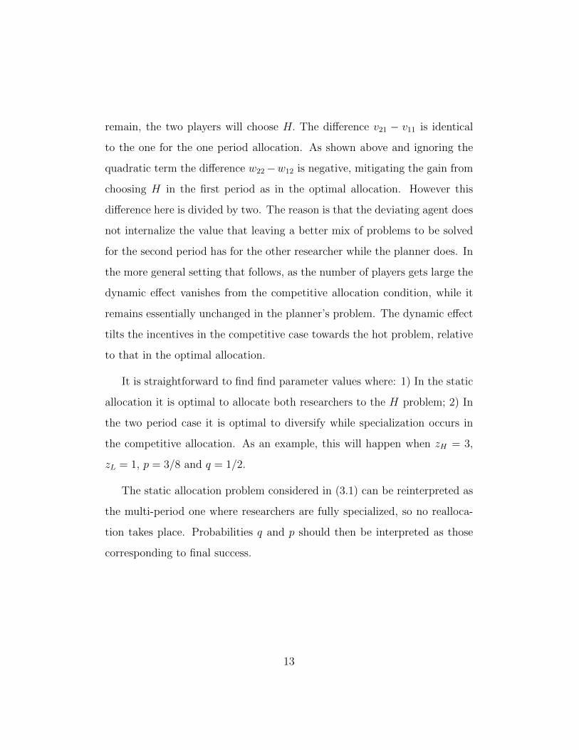
quadratic term the difference w22−w12 is negative, mitigating the gain from

choosing H in the first period as in the optimal allocation. However this

difference here is divided by two. The reason is that the deviating agent does

not internalize the value that leaving a better mix of problems to be solved

for the second period has for the other researcher while the planner does. In

the more general setting that follows, as the number of players gets large the

dynamic effect vanishes from the competitive allocation condition, while it

remains essentially unchanged in the planner’s problem. The dynamic effect

tilts the incentives in the competitive case towards the hot problem, relative

to that in the optimal allocation.

It is straightforward to find find parameter values where: 1) In the static

allocation it is optimal to allocate both researchers to the H problem; 2) In

the two period case it is optimal to diversify while specialization occurs in

the competitive allocation. As an example, this will happen when zH = 3,

zL = 1, p = 3/8 and q = 1/2.

The static allocation problem considered in (3.1) can be reinterpreted as

the multi-period one where researchers are fully specialized, so no realloca-

tion takes place. Probabilities q and p should then be interpreted as those

corresponding to final success.

13

4 Assignment without Reallocation

In this Section we lay out the basic model used in the rest of the paper and

consider a general form of the static allocation problem discussed in Section

3.1.

There is a large number (in fact, a continuum) of problems or R&D lines,

with one potential innovation each. Upon discovery, an innovation delivers

value z that is distributed across research lines with cumulative distribution

function F, which we assume to be twice differentiable. To isolate the findings

of this paper from the well-known effects discussed earlier, we assume that

the social value of an innovation coincides with the private value z.7 There

is a mass M > 0 of researchers, who are allocated to the different R&D

lines according to a measurable function m. The technology of discovery is

given by a function P (m) that is strictly increasing, concave and identical

for all problems and P (0) = 0. For each innovation of value z, we denote by

m(z) the mass of researchers competing for the discovery of that innovation.

Hence, the resource constraint∫∞

0m (z) dF (z) ≤M needs to be satisfied.

The expected payoff of participating in an R&D line with value z and

a total of m (z) researchers is given by U (z,m (z)) = P (m (z)) z/m (z).

As we show below, these payoffs can be interpreted as a winner-take-all

7The expected present discounted value zj of the patented innovation j does not neces-sarily equal the market profit for the patented product, net of development and marketingcosts. It may also include the expected license fees paid by other firms which marketimprovements in the future, or the profit for innovations covered by continuation patents.Thus, our model is compatible with standard sequential models of innovation, both thoseassuming that new innovations do not displace earlier ones from the market, as in themodels following Green and Scotchmer (1995), and those assuming the opposite, as in thequality ladder models that follow Aghion and Howitt (1992).

14

patent race where all participating researchers have equal probability of being

first to innovate. Our model can thus be interpreted as an extension of the

standard patent race to multiple lines. While that literature considers a

single race with a perfectly elastic supply of researchers/firms with some

entry/opportunity cost, we consider here the opposite extreme where a fixed

supply of research inputs M must be allocated across multiple innovations.

8

In a competitive equilibrium expected payoffs P (m (z)) z/m (z) are equal-

ized among all active lines, where m (z) > 0. We call this differential rent

dissipation in analogy to absolute rent dissipation in the standard patent

race literature. In contrast, in the optimal allocation m (z) that maximizes

W (m) =∫∞

0zP (m (z)) dF (z), the marginal contributions P ′ (m (z)) z are

equalized for all active lines.

In a competitive equilibrium, a marginal researcher contributes P ′ (m) z

to total value but gets a return P (m) z/m which is greater, as a result of

the concavity of P. The difference P (m) z/m − P ′ (m) z is the pecuniary

externality inflicted on competing innovators. Relative to the value created,

this externality is given by:

P (m (z))

P ′ (m (z))m (z)− 1 =

1

εPm− 1 (3)

where the first term corresponds to the inverse of the elasticity of discovery

with respect to the number of researchers. It is immediate to see that the

8Obviously with perfectly elastic supply the problem trivializes as there would be noconnection between entry decisions into different research areas. We consider the oppositeextreme to emphasize the tradeoff in allocating research inputs across different researchlines, but our results should also hold for intermediate cases.

15

Figure 1: Bias to High z areas

z

mm(z)

m(z)~

*

competitive allocation will be optimal if and only if this external effect is the

same across research lines. Given that differential rent dissipation implies an

increasing function m (z) , this condition will hold only when the elasticity of

discovery is independent of m, i.e. when the discovery function P (m) = Amθ

for some constant A.9

When this condition does not hold, the direction of the bias will depend on

how this external effect varies with m. Intuitively, when it increases (i.e. the

elasticity of the discovery function is decreasing in m) there will be excessive

concentration in high z areas, as we show below. We say that the competitive

equilibrium is biased to higher z (“hot”) research lines when the competitive

and optimal allocations m (z) and m (z) have the single crossing condition

shown in Figure 1. Formally, there exists a threshold z such that m (z) <

9Note, however, that since P is bounded by 1 this function can only hold for a rangewhere mθ ≤ 1/A and beyond this range the elasticity must be zero.

16

m (z) for z < z and m (z) > m (z) for z > z. Further, when this condition

holds, it is also the case that the smallest active R&D line innovation value

is higher in equilibrium than in the first best; i.e., that z0 = infz{m (z) >

0} ≤ z0 = infz{m (z) > 0}. The following Proposition gives conditions for

this to hold.

Proposition 1. In the absence of reallocation, the competitive equilibrium is

biased to higher z areas when the elasticity of discovery is decreasing in m.

Proof. See Appendix.

While the condition in this Proposition might appear somewhat special, it

holds in the canonical model of innovation used in the patent race literature,

as we show below. Moreover, as P (m) /m is bounded by 1, the elasticity

must converge to zero as m→∞ so it must decrease in some region.

Stationary Innovation Process

The above setting can be inscribed in a dynamic environment as follows. Let

t denote the random time of discovery and p (t;m) the corresponding density

when m researchers are assigned from time zero to this research line. The

expected utility for each of them is given by

U (zj;mj) =

∫ ∞0

( zm

)e−rtjp (t;m) dt.

Expected payoffs are divided by m since each innovator is equally likely

to win the race and if m researchers are engaged in a particular research

line, p (t,m) denotes the density of discovery at time t. Letting P (m) ≡

17

E [e−rt;m] =∫∞

0e−rtp (t;m) dt, we can write U (z;m) = zP (m)/m, which is

identical to the formulation given above. It is important to emphasize that

while time is involved in the determination of payoffs, we are assuming here

that once discovery takes place, the m researchers involved become idle and

cannot be reallocated to other research lines. The following sections relax

this assumption and considers explicitly the problem of reallocation.

We specialize now the setting to a stationary environment that is used in

the remainder of the paper. Let λ (m)m denote the hazard rate for discovery

at any moment of time so that p (t,m) = λ (m)me−λ(m)mt. Assume that

λ (m)m is increasing, concave and that λ (0) = 0. It follows easily that

P (m) =λ (m)m

r + λ (m)m

and the elasticity

εPm =

(r

r + λ (m)m

)(1− ελm)

where where ελm denotes the elasticity of λ with respect tom, −λ′ (m)m/λ (m)

It immediately follows that

Proposition 2. If the elasticity ελm is weakly increasing in m the competitive

allocation will be biased to high z lines.

We can interpret the elasticity ελm as the market stealing externality per

unit of value created: λ (m)m/λ′(m) . The condition given in the Proposition

then states that this externality increases with z. Note also that this is a

sufficient but not necessary condition, as the first term is decreasing in m.

The Proposition applies to the canonical R&D models as the ones discussed

in the literature, where λ (m) = λm (i.e. discovery is independent across

18

participants in a patent race) and the elasticity ελm = 1. Each active research

line can be thus interpreted as a patent race, where arrival rates given by

independent Poisson processes with rate λ and the first to innovate gets the

rights to the full payoff z. More generally, the result applies for the constant

elasticity case where λ (m) = λm−θ for 0 ≤ θ < 1. For the canonical model

of patent races where θ = 0, an explicit solution for the equilibrium and

optimal allocations is given below.

Proposition 3. Suppose that there is a continuum of R&D lines, whose

innovation discoveries are independent events, equally likely among each en-

gaged researcher, with time constant hazard rate λ. Then, the equilibrium and

optimal allocation functions are

m (z) =z − z0

π, for all z ≥ z0 = rπ/λ (4)

m (z) =r

λ

(√z

z0

− 1

), for z ≥ z0 = rµ/λ, (5)

where π is the equilibrium profit of each R&D line, and µ is the Lagrange

multiplier of the resource constraint. In equilibrium, innovators over-invest

in the hot R&D lines relative to the optimal allocation of researchers: there

exists a threshold z such that m (z) < m (z) for z < z and m (z) > m (z) for

z > z.

Importantly, this result demonstrates the market bias that is the theme

of this paper (that competing firms over-invest in hot R&D lines) within a

canonical dynamic model directly comparable with the many R&D models

since Loury (1979) and Reinganum (1981), that are built on the assumption

of exponential arrival of innovation discoveries.

19

Figure 2: Plot of the welfare wedge W (m) /W (m) .

To get a sense of the possible size of this distortion, we perform a sim-

ple back-of-the-envelope calculation. Supposing that innovation values are

distributed according to a Pareto distribution of parameter η > 1, so that

F (z) = 1 − z−η for z ≥ 1. As proved in Appendix B, when λ (m) = λ and

η > 1, in an interior allocation where z0 > 1, the welfare gap is:

W (m)

W (m)=

η

η − 1

(η − 1

2η − 1

)1/η

.

This ratio is plotted in Figure 2. It is negligible for η close to 1, but

quickly increases as η grows, so that W (m) /W (m) − 1 reaches its maxi-

mum of about 20% for η close to 1.35 to then slowly decrease and disappear

asymptotically as η →∞. Figure 3 gives the corresponding equilibrium and

optimal allocations. The solid line corresponds to the optimal allocation and

the dashed line to the equilibrium.

We have assumed here that arrival rates are the same for all research

lines. Our results can be extended for heterogeneity where the attractiveness

20

Figure 3: Equilibrium and Optimal Allocation (η = 1.35)

of R&D lines is not determined only by the innovations’ expected market

values, but also by the ease of discovery.

[Francesco: Should we do more of that here: formula showing low hanging

fruit?]

5 Dynamic Allocation

We extend our previous analysis by allowing the mobility of researchers once

a research line is completed. As before, we assume there is a unit mass of

research areas (the problems to be solved) with continuous distribution F (z)

and there is an inelastic supply M of researchers. While here the set of prob-

lems is fixed, Section 6 considers a steady state with entry of new problems.

Throughout this section we assume that λ (m) is twice continuously differen-

tiable, λ (m)m is strictly increasing and strictly concave and that λ (0) = 0.

These assumptions imply that the arrival rate per researcher λ (m) is de-

21

creasing, i.e. there is instantaneous congestion.10 Researchers are free to

move across different problems so the equilibrium and optimal allocations

determine at any time t the number of researchers m (t, z) assigned to each

line of research z. This assignment, together with the results of discovery

imply an evolution for the distribution of open problems G (t, z), where

∂G (t, z) /∂z = −∫ z

λ (m (t, s))m (t, s)G (t, ds) (6)

with G (0, z) = F (z) . An allocation is feasible if at all times the resource

constraint: ∫m (t, z)G (t, dz) ≤M (7)

is satisfied.

Equilibrium

Because the set of undiscovered innovations shrinks over time, it is never the

case that innovators choose to move across R&D lines in equilibrium, nor

that it is optimal to do so, unless the R&D line in which the researchers are

engaged is exhausted as a consequence of innovation discovery. Indeed, the

mass of researchers assigned to a particular line or research z will increase

over time. Because mobility is free, the value of participating in any research

10Strict concavity implies that the arrival rate does not scale linearly with innovation,which can also capture duplication of innovation effort. In the process of achieving apatentable innovation, competing innovators often need to go through the same interme-diate steps (see, for example the models of Fudenberg et al., 1983, and Harris and Vickers,1985), and this occurs independently of every other innovators’ intermediate results, thatare jealously kept secret. Hence, the arrival rate of an innovation usually does not doubleif twice as many innovators compete in the same R&D race.

22

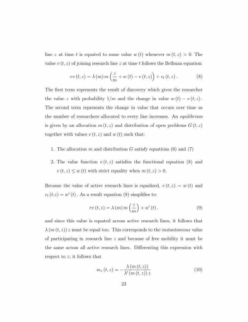
line z at time t is equated to some value w (t) whenever m (t, z) > 0. The

value v (t, z) of joining research line z at time t follows the Bellman equation:

rv (t, z) = λ (m)m( zm

+ w (t)− v (t, z))

+ vt (t, z) . (8)

The first term represents the result of discovery which gives the researcher

the value z with probability 1/m and the change in value w (t) − v (t, z) .

The second term represents the change in value that occurs over time as

the number of researchers allocated to every line increases. An equilibrium

is given by an allocation m (t, z) and distribution of open problems G (t, z)

together with values v (t, z) and w (t) such that:

1. The allocation m and distribution G satisfy equations (6) and (7)

2. The value function v (t, z) satisfies the functional equation (8) and

v (t, z) ≤ w (t) with strict equality when m (t, z) > 0.

Because the value of active research lines is equalized, v (t, z) = w (t) and

vt (t.z) = w′ (t) . As a result equation (8) simplifies to:

rv (t, z) = λ (m)m( zm

)+ w′ (t) . (9)

and since this value is equated across active research lines, it follows that

λ (m (t, z)) z must be equal too. This corresponds to the instantaneous value

of participating in research line z and because of free mobility it must be

the same across all active research lines. Differenting this expression with

respect to z, it follows that

mz (t, z) = − λ (m (t, z))

λ′ (m (t, z)) z(10)

23

This equation can be integrated starting at a value z0 (t) where m (t, z0 (t)) =

0 and z0 (t) is the unique threshold where the resource constraint∫z0(t)

m (t, z (t))G (t, dz) = M (11)

is satisfied. As the mass of G decreases over time, it also follows that the

threshold z0 (t) decreases.

Proposition 4. The equilibrium allocation is the unique solution m (z) that

satisfies equation (10) and m (t, z) > 0 iff z > z0 (t) , where the threshold

z0 (t) satisfies equation (11).

Optimal Allocation

Consider an allocation m (t, z) .At time t this gives a flow of value λ (m (t, z)) z.

Integrated over all active research lines and time periods, gives the objective:

U = maxm(t,z)

∫e−rt

∫λ (m (t, z)) m (t, z) zG (t, dz) dt (12)

The optimal allocation maximizes (12) subject to the resource constraint (7)

and the law of motion (6). The latter is more conveniently expressed by the

change in the density

∂g (t, z) /∂t = −λ (m (t, z))m (t, z) .

The formal expressions for the Hamiltonian are given in Appendix C. Letting

u (t) denote the multiplier of the resource constraint and v (t, z) the one

corresponding to this law of motion, we can write the functional equation:

rv (t, z) = maxm

λ (m) m [z − v (t, z)]− u (t) m+ vt (t, z) (13)

24

for all z ≥ z0 (t) .

Equation (13) represents the value of an unsolved problem of type z at

time t. It emphasizes that problems are indeed an input to innovation, and

as can be easily shown the value of an open problem increases with z. Note

the contrast to the private value v (t, z) that is equal for all z as a result

of the differential rent dissipation: in the eyes of competing innovators, all

problems become equally attractive and valuable. The value function defined

by (13) can also be interpreted as part of a decentralization scheme where

property rights are assigned for each problem z and the owner of each open

problem chooses the number of researchers to hire at a rental price u (t) . This

interpretation highlights the source of market failure in our model precisely

due to the lack of such property rights.

The solution to the maximization problem in equation (13) gives:

[λ′ (m (t, z)) m (t, z) + λ (m (t, z))] [z − v (t, z)] = u (t) (14)

Comparing to the equilibrium condition where λ (m (t, z)) z is equalized, re-

veals the two key sources of market failure that were illustrated in our simple

example in Section 3. First is that the planner internalizes congestion (i.e.

the market stealing effect) that is why payoffs are multiplied and not just by

the arrival rate λ. It is useful to rewrite the term in brackets as:

λ (m (t, z)) [1− ελm] (15)

Note the parallel to the results in the case without reallocation considered

in Section 4, where the term in brackets corresponds to the wedge between

the optimal and competitive allocation. The second term in brackets in

25

equation (14) captures the fact that the payoff for discovery is smaller for

the social planner as it internalizes the fact that a valuable problem is lost as

a consequence, as we found in our simple example. Taking the ratio of the

two conditions gives:

λ (m (t, z))

λ (m (t, z))= (1− ελm (m (t, z)))

(z − v (t, z)

z

)v (t)

u (t)

For fixed t, the allocation functions cross when λ (m (t, z)) = λ (m (t, z)) .

Since the λ function is decreasing, a sufficient condition for m (t, z) to re-

main higher after crossing is that this ratio decreases with z. This is the

composition of two effects, represented by the two terms in brackets above.

The first term is decreasing if the elasticity is increasing in z, i.e. the mar-

ket stealing effect increasing. Because the value function is convex in z, the

second term decreases in z. This corresponds to the option value effect that

we found in our simple example. We have proved:

Proposition 5. Consider the model with free research mobility with individ-

ual arrival rate λ (m). Suppose that the elasticity ελm is weakly increasing in

m. Then, in equilibrium, innovators over-invest in the hot R&D lines: there

exists a twice differentiable threshold function z such that m (t, z) < m (t, z)

for z < z(t) and m (t, z) > m (t, z) for z > z(t).

Note that even abstracting from the first effect (e.g. when the elasticity

is constant) the competitive bias to hot areas still holds.

A borderline case occurs in the absence of congestion, i.e. where λ (m) =

λ and total arrival is linear in λ. Since there is no force to equalize rents

in the competitive case, the solution is extreme and all researchers join the

26

highest remaining payoff line at any point in time. The same turns out to

be true in the optimal allocation, so in this knife-edge case the equilibrium

is efficient. Reallocation costs provide an alternative rent equalizing force

that can lead to a non-degenerate equilibrium. These are examined in the

following section.

Costly Reallocation

Assume that in the stationary dynamic model discussed above λ (m) = λ.

Suppose that, at any point in time, each researcher can be moved across

research lines by paying an entry cost c > 0. For every innovation of value

z and time t, we denote the mass of engaged researchers as m (t, z) , and

let z0(t) to be the smallest active R&D line innovation value at time t; i.e.,

z0(t) = infz{m (t, z) > 0}. An equilibrium is defined in the same way as done

in the previous section.

Because the set of undiscovered innovations shrinks over time, there is

positive entry into any active line of research, so it is never the case that

innovators choose to move resources across R&D lines in equilibrium, nor

that it is optimal to do so, unless the R&D line in which the researchers

are engaged is exhausted as a consequence of innovation discovery.11 So,

we can approach again the problem using standard dynamic programming

techniques. We express the equilibrium value v (t, z) of a researcher engaged

11Further, as we show in Proposition 6 below, there exists a time T after which re-searchers are not redeployed into other R&D lines, even when their research line is ex-hausted due innovation discovery.

27

in a R&D line of innovation value z at t through the Bellman equation:

rv (t, z) = λm (t, z)

[z

m (t, z)+ w (t)− v (t, z)

]+d

dtv (t, z) . (16)

The flow equilibrium value rv (t, z) includes two terms. The first one is

the expected net benefit due to the possibility of innovation discovery. The

hazard rate of this event is λm (t, z); if it happens, each researcher gains z

with probability 1/m (t, z) and experiences a change in value w (t)− v (t, z)

where w (t) represents the value of being unmatched. The second term,

ddtv (t, z) , is the time value change due to the redeployment of researchers

into the considered R&D line from exhausted research lines with discovered

innovations.

For any time t, both the equilibrium value v (t, z) and its derivative

ddtv (t, z) are constant across all active R&D lines of innovation value z ≥

z0(t).12 Let v(t) and v′(t) denote these values. In addition, note that since

an unmatched researcher can join any research line at cost c, it follows that

v (t) = u (t) + c. Substituting in (16) we obtain the no-arbitrage equilibrium

condition:

λ [z −m (t, z) c] = rv(t)− v′(t), for all z ≥ z0(t). (17)

implying that z −m (t, z) c is equated across all active research lines. Given

that m (t, z) ↓ 0 as z ↓ z0, it follows that payoffs of all active lines z−m (t, z)

12These conditions are akin to value matching and smooth pasting conditions in stoppingproblems (for example, see Dixit and Pindyck, 1994). Because R&D firms are competitive,and labor is a continuous factor, the equilibrium dissipates all value differences from dis-covery of different innovations, through congestion and costly redeployment of researchers.This is similar to the phenomenon of rent dissipation in models of patent races with costlyentry.

28

are equated to z0 : differential rents are dissipated through higher entry

rates in higher return areas, being all equated to the lowest active value line.

Notice the parallel to the results in the patent race literature, where all rents

are dissipated through entry. It follows that the flow value in the economy

at time t is λMz0 (t) .

Solving for m (t, z) using the above gives

m (t, z) = [z − z0(t)] /c, for all z ≥ z0(t) (18)

When the resource constraint∫∞z0(t)

m (t, z) dG (t, z) ≤ M binds, the initial

condition z0(t) is pinned down by the equation:

cM = c

∫ ∞z0(t)

m (t, z) dG(t, z) =

∫ ∞z0(t)

(z − z0 (t)) dG (t, z) , (19)

where G (t, z) is again the cumulative distribution function of innovations

not discovered yet at time t.

We also note that, because active R&D lines with innovation value z ≥

z0(t) get exhausted over time, more researchers engage in the remaining lines,

i.e., mt(t, z) > 0 for all z ≥ z0(t); less valuable lines becoming active, i.e.,

z′0(t) < 0, and each active research line becomes less valuable, i.e., v′(t) < 0.

Indeed, the value v(t) decreases over time until the time T such that v(T ) = c.

At that time, redeployment of researchers stops at the end of the R&D race

in which they are engaged. Active research lines have become so crowded

that their value is not sufficient to recover the entry cost c any longer.13

13The characterization of the allocation m(t, z) of researchers on undiscovered R&Dlines at any time t ≥ T is covered by the earlier analysis of the canonical dynamic modelwithout redeployment of researchers (cf. Proposition 3). In our set up with a continuum ofR&D lines distributed according to the twice differentiable function G, arguments invoking‘laws of large number’ suggest that the allocation m(t, z) would smoothly converge to theallocation m(t) described in Proposition 3.

29

The next Proposition summarizes the above equilibrium analysis.

Proposition 6. Assume λ (m) = λ and that researchers can be moved across

R&D lines at cost c > 0. The equilibrium allocation:

m (t, z) =z − z0(t)

c, for all z ≥ z0(t), (20)

where the boundary z0(t) solves equation (19). Researchers are redeployed

into different active R&D lines only until the time T such that z0(T ) = rc/λ,

and only if their research line is exhausted due to innovation discovery. The

flow value in the economy at time t is λMz0(t).

We now consider the optimal allocation that is defined as in the previous

section, after subtracting total entry costs. Following the same approach, we

solve for the optimal allocation m using the Bellman equation defined by the

co-state dynamic condition in the Hamiltonian. The details are provided in

Appendix C. The value of a research line z at time t satisfies

rv (t, z, 0) = maxm∈R

λm [z − v (t, z, m)]−rmc−u (t) m+vt (t, z, m) , for all z ≥ z0(t).

(21)

There are several comments to make about this equation. First, note that

due to the irreversible entry cost c, the value function has as an additional

argument the number of researchers m. On the left hand side we consider

the flow value of an empty research line with m = 0. On the right hand

side we consider the optimal choice of m. The entry cost mc is expressed in

flow terms consistent with the formulation of the value function. As before

u(t) is the multiplier for the resource constraint. Finally note that at the

optimal choice v (t, z, m (t, z)) = v(t, z, 0) + m (t, z) c. This also implies that

30

vt (t, z,m) is independent of m, which is used below. Substituting in (21) we

obtain:

rv (t, z, 0) = maxm∈R

λm [z − v (t, z, 0)−mc]−rmc−u (t) m+vt (t, z, m) , for all z ≥ z0(t).

(22)

This can be also interpreted as the Bellman equation for a firm that is as-

signed the property rights to a problem z at time t and needs to choose

the initial amount of researchers to hire, paying the initial entry cost mc

and rental price u (t) . The solution of program (21) leads to the first order

conditions:

λ [z − v (t, z, 0)− 2m(t, z)c] = rc+ u (t) , for every z ≥ z0(t). (23)

Equating these first order conditions leads to the differential equation

mz (t, z) =1− vz (t, z, 0)

2c. (24)

By comparison, the differential equation for the equilibrium allocation ob-

tained by differentiating (18) gives:

mz (t, z) =1

c. (25)

It follows immediately that the derivative mz of the optimal allocation func-

tion m is smaller than mz, the derivative of the equilibrium allocation func-

tion m.14 Because both functions m and m need to satisfy the same resource

allocation constraint, this implies that the competitive equilibrium is biased

towards high return areas.

14We prove in the appendix that 0 < vz (t, z) < 1.

31

Further, the comparison of equations (24) and (25) allows us to single

out two separate effects that lead to this result. First, is the option value

effect described earlier, where the marginal value of a better research line is

1− vz which is less than one, the marginal value in the competitive equilib-

rium. The derivative vz captures the fact that a better problem has also more

value in the future, in contrast to equalization due to rent dissipation that

occurs in the competitive case. As a result, when engaging in a R&D line of

value z, competing firms do not internalize the negative externality vz (t, z) ,

the change in the continuation value due to the reduced likelihood of discov-

ering the innovation later. This leads the competing firms to sub-optimally

anticipate investment in the hot R&D lines, leading to over-investment at

every time t.

At the same time, the additional social marginal cost for engaging an ad-

ditional researcher in a marginally more profitable line, 2c · mz (t, z) , is twice

the private additional expected cost c · mz (t, z) incurred by the individual

researcher. On top of this private cost, the society suffers also an additional

redeployment cost. This cost is incurred in expectation by all researchers

already engaged in the more profitable R&D line, in case the additional

researcher wins the R&D race. This additional redeployment cost is not in-

ternalized by the competing firms, and it also pushes towards equilibrium

over-investment in the hot R&D lines.15

15The result that R&D firms overinvest in hot R&D lines fails to hold only when c = 0(the case of perfectly costless redeployment of researchers). In this case, assuming thatthe innovation value distribution has bounded support, all researchers will be first engagedin the most valuable R&D lines. When these innovation are discovered, they will all beredeployed to marginally less valuable ones, until also these innovations are discovere, andso on and so forth. This unique equilibrium outcome is also socially optimal.

32

Proposition 7. Assume λ (m) = λ and there is a cost of entry c > 0 to start

solving any new problem. Then, in the competitive equilibrium innovators

over-invest in high return R&D lines at every time t: there exists a threshold

function z(t) such that m (t, z) < m (t, z) for z < z(t) and m (z) > m (t, z)

for z > z(t).

The following section extends this model by considering the arrival of new

R&D lines.

6 Steady State Economy

Consider the model analyzed in the last section and suppose in addition new

problems arrive with Poisson intensity α and returns z distributed according

to an exogenous distribution F (z) . We focus on R&D line replacement that

keeps the economy in steady state.16

In steady state, the equilibrium allocation m is independent of time t, and

thus calculated with obvious modifications of the analysis presented earlier

in this section. The expression λ [z −m (z) c] is constant for all z ≥ z0, so

that the equilibrium solves the differential equation m′(z) = 1/c, which gives

the solution

m (z) = (z − z0)/c, for every z ≥ z0. (26)

Likewise, obvious modifications of the Bellman equations (21) shows that the

16For simplicity, we assume that when an innovation is discovered, the cost c for re-deploying researchers is the same for all R&D lines, including the follow up lines of theinnovation discovery. Our results would extend to a more complicated model in which theredeployment cost is smaller for these lines as long as they are not exactly equal to zero.

33

social planner problem takes the following form, in steady state:

rv (z) = maxm∈R

λm [z − v (z)− mc]− rmc− um, for all z ≥ z0, (27)

under the constraint that u satisfies the resource constraint. The associated

first-order conditions are:

λ [z − v (z)− 2m(z)c] = rc+ u, for every z ≥ z0. (28)

Inspection of the equilibrium condition and equation (27) reveal the same

two forces identified earlier leading to excessive equilibrium investment in

hot areas, so there exists a threshold z such that m (z) < m (z) for z < z,

and m (z) > m (z) for z > z.

With simple manipulations presented in appendix B, we obtain:

λ

[z − cλm(z)2

r− 2c · m(z)

]= rc+ u, for every z ≥ z0. (29)

These equations are analogous to the ones obtained in the first-order con-

ditions (23) for the model redeployment that we solved earlier. The only

difference is that the term v (z) takes the constant form c · λm(z)2/r, here,

which is the discounted cost of all future redeployment of the mass m (z) of

researchers engaged in the considered R&D line —the term c ·λm(z)/r is the

individual discounted cost. So, we can identify as c ·λm(z)2/r+ c · m(z), the

‘redeployment cost externality’ that an additional researcher imposes on the

m (z) researchers engaged in the R&D line. As shown in appendix B, equa-

tion (29) can be used to obtain an explicit solution for the optimal allocation

as a function of z0 :

m (z) =r

λ

(√λz − z0

rc+ 1− 1

), for all z ≥ z0. (30)

34

17

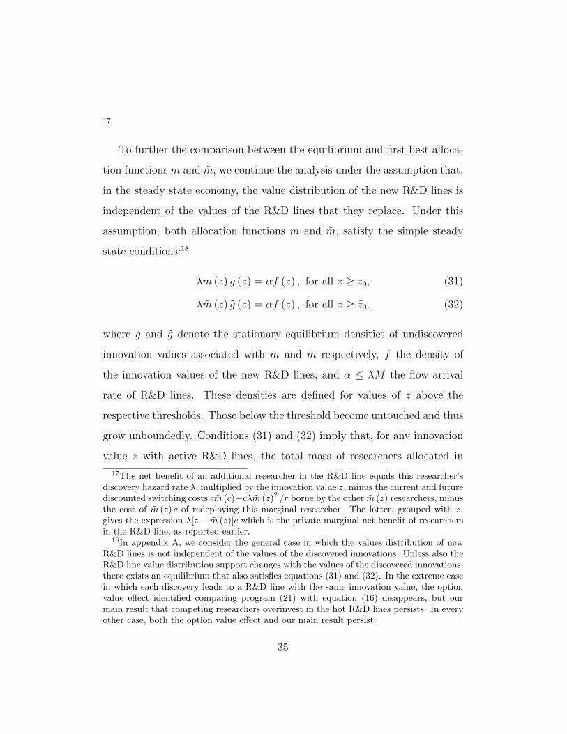
To further the comparison between the equilibrium and first best alloca-

tion functions m and m, we continue the analysis under the assumption that,

in the steady state economy, the value distribution of the new R&D lines is

independent of the values of the R&D lines that they replace. Under this

assumption, both allocation functions m and m, satisfy the simple steady

state conditions:18

λm (z) g (z) = αf (z) , for all z ≥ z0, (31)

λm (z) g (z) = αf (z) , for all z ≥ z0. (32)

where g and g denote the stationary equilibrium densities of undiscovered

innovation values associated with m and m respectively, f the density of

the innovation values of the new R&D lines, and α ≤ λM the flow arrival

rate of R&D lines. These densities are defined for values of z above the

respective thresholds. Those below the threshold become untouched and thus

grow unboundedly. Conditions (31) and (32) imply that, for any innovation

value z with active R&D lines, the total mass of researchers allocated in

17The net benefit of an additional researcher in the R&D line equals this researcher’sdiscovery hazard rate λ, multiplied by the innovation value z, minus the current and futurediscounted switching costs cm (c)+cλm (z)

2/r borne by the other m (z) researchers, minus

the cost of m (z) c of redeploying this marginal researcher. The latter, grouped with z,gives the expression λ[z − m (z)]c which is the private marginal net benefit of researchersin the R&D line, as reported earlier.

18In appendix A, we consider the general case in which the values distribution of newR&D lines is not independent of the values of the discovered innovations. Unless also theR&D line value distribution support changes with the values of the discovered innovations,there exists an equilibrium that also satisfies equations (31) and (32). In the extreme casein which each discovery leads to a R&D line with the same innovation value, the optionvalue effect identified comparing program (21) with equation (16) disappears, but ourmain result that competing researchers overinvest in the hot R&D lines persists. In everyother case, both the option value effect and our main result persist.

35

the steady state equilibrium and optimal allocations, respectively m (z) g (z)

and m (z) g (z) , are both equal to (α/λ) f (z) , the net inflow of R&D lines

of innovation value z. Of course, this does not mean that also the mass of

researchers engaged in each R&D line is the same: it need not be that m(z) =

m (z) for any active R&D line of innovation value z since the stationary

distributions g and g will differ.

We now turn to the determination of the thresholds. Assuming the re-

source feasibility constraint∫ +∞z0

m (z) g (z) dz ≤ M binds in both alloca-

tions, the threshold z0 is pinned down by plugging the stationarity condition

(31) into the binding resource constraint, so as to obtain the equation

α (1− F (z0)) = λM. (33)

Again λM is the outflow of solved problems which must equal in steady

state the inflow of new relevant problems. Remarkably, this implies that the

threshold z0 is determined independently of the allocation function m, so in

particular z0 = z0. Equations (26), (30) and (33) can be used to solve for the

equilibrium and optimal allocations. 19

Because the thresholds z0 and z0 coincide, mz > mz and limz↓z0 m (z) =

limz↓z0 m (z) = 0, it follows that m(z) > m (z) for all z > z0. This is consis-

tent with both allocations integrating to total resources M precisely because

the stationary distribution of open problems G in the optimal allocation

stochastically dominates G, the one in the stationary competitive equilib-

rium.

19If the resource constraint is satisfied with a strict inequality,∫∞z0m (z) dG (z) < M,

then the economy cannot support entry by all firms, the participation constraint v ≥ cbinds and pins down z0 through the equality c = v = (λ/r)z0.

36

In words, the density of the R&D lines with undiscovered innovations is

very large for small innovation values, very few researchers are engaged on

these R&D lines, and hence innovation discoveries arrive with a very low

rate. As the innovation value grows larger, the density of R&D lines with

undiscovered innovations decreases. The rate of decrease is larger for the

competitive equilibrium than for the optimal allocation function. So, the

market sub-optimally exhausts too many high value R&D lines too early,

and leaves too few for future discovery. As a consequence of this, the number

of researchers per project is always higher in equilibrium than in the social

optimum, because the there are more high-value R&D lines in the social

optimum, and these high-value R&D lines take up more researchers than low

value R&D lines.

Welfare

In any allocation m (z) the flow of value

rV = λ

∫z0

m (z) (z −m (z) c) g (z) dz

= α

∫z0

(z −m (z) c) f (z) dz. (34)

= α

∫z0

zf (z) dz − αc∫z0

m (z) f (z) dz

The first term is the same in any allocation and it is precisely the value

of the outflow of problems solved that in a stationary equilibrium equals

the corresponding inflow. Since the latter is independent of the allocation,

so is the former. The second term corresponds to the total flow costs of

redeployment, that differs across the two allocations. In the competitive

37

allocation cm (z) = (z − z0) . Substituting in the equation above gives:

rV = α

∫z0

zf (z) dz − α∫z0

(z − z0) f (z) dz

= αz0 (1− F (z0)) = λMz0.

This represents a value equivalent to the flow of all innovations equalized

to the lowest value one, reflecting again differential rent dissipation. Note

that as z0 is independent of c, this value is the same for all c, within a range

where all researchers are employed in the steady state. In particular, it holds

surprisingly even as c ↓ 0 due to tan unboundedly increasing concentration

in high return areas.

Consider now the flow value of the optimal allocation. Using (30), it

follows that

αm (z) f (z) c =rα

λ

(√cλ

(z − z0)

r+ c2 − c

)f (z) .

Substituting in (34) and using our previous result proves:

Proposition 8. When λ (m) = λ, the cost of entry is c > 0 and the flow of

entry of new problems α with density f, aggregate equilibrium and optimal

welfare are given, respectively by:

W (m) = (λ/r)z0M (35)

and

W (m) =α

r

∫ ∞z0

zf (z) dz + cM − α

λ

∫ ∞z0

√cλ

r(z − z0) + c2 · f (z) dz. (36)

These closed-form expressions make welfare assessments simple and pre-

cise. Welfare is dissipated in the equilibrium allocation with excess researcher

38

turnover to equal the flow of the lowest active research area. The reason why

the welfare is not dissipated in the optimal solution is because the social

planner spreads out researchers more evenly and leaves a larger number of

hot R&D lines for later, so that the society does not pay as much in terms

of relocation costs.

When the switching costs are small, the optimal welfare expression sim-

plifies further:

limc→0+

W (m) = (α/r)

∫ ∞z0

zf (z) dz = (α/r)E (z|z ≥ z0) [1− F (z0)]

= (λ/r)E (z|z ≥ z0)M.

Again, this result makes transparent the comparison between rent dissipation

in the competitive equilibrium that is not present in the planner’s solution.

Thus, for small switching cost c, the welfare ratio W (m)/W (m) takes the

form:

limc→0+

W (m)

W (m)=

z0

E (z|z ≥ z0).

In words, the welfare ratio converges to the smallest active R&D line inno-

vation value z0, divided by the expected active R&D line innovation value.

It is intuitive that this quantity can be significantly small, for standard cu-

mulative distributions F.20

20We performed a back-of-the-envelope calculation of the welfare ratio W (m)/W (m),under the assumption that the distribution F is lognormal with mean equal to 7 andstandard deviation equal to 1.5, consistently with the estimates provided by Schankerman(1998). With cost c = 1 million, the welfare ratio W (m)/W (m) is approximately 0.28. Asthe cost c vanishes, the ratio W (m)/W (m) converges to 0.17 approximately.

39

7 Conclusion

Research on the efficiency of innovation markets is usually concerned on

whether the level of innovator investment is socially optimal. This paper has

asked a distinct, important question: Does R&D go in the right direction?

In a simple dynamic model, we have demonstrated that R&D competition

pushes firms to disproportionately engage in the hot research lines, charac-

terized by higher expected rates of return. The identification of this form of

market failure is a novel result, as we explained in details in the introduction

and literature review.

After demonstrating this result within a simple model, we have extended

our framework in different directions, so as to include various features of

economic interest. The canonical dynamic model we have formulated is pop-

ulated with a continuum of innovation R&D lines, whose discovery is an

independent random event, equally likely across all engaged researchers, and

with time-constant hazard rate. We have allowed for both possibilities that

researchers may or may not be moved across R&D lines costly. We have

studied the case in which the innovation discovery hazard rate grows with

the number of engaged researchers proportionally, and the case in which it

grows less than proportionally because of duplicative R&D effort. We have

worked both under the assumption that R&D lines that are exhausted due to

innovation discovery may not be replaced by successive innovation vintages,

and under the assumption that they are replaced, so as to keep the economy

in steady state.

We have recovered the result that competing innovators overinvest in

40

the hot research areas in all cases, with the exception of the knife-hedge

case without duplicative R&D effort, without R&D line replacement, and in

which researchers can be switched across R&D line costlessly. Importantly,

this analysis allowed us to clarify which specific features of R&D competition

lead to the market failure that is the theme of this paper. The analysis for

the case in which the economy is in steady state has also allowed us calculate

the equilibrium and optimal welfare expressions in simple closed forms.

To offset the distortion that competing innovators overinvest in the hot

research lines in equilibrium, a simple policy recommendation is that R&D

lines with less profitable or less feasible innovations are subsidized, so as to

rebalance remuneration across R&D lines. Importantly, our case for R&D

subsidization is based on a framework without any market frictions. We argue

that even frictionless markets and competition forces cannot solve the form

of market failure identified here. And in fact, we have shown that increasing

market competition can only make the equilibrium distortion worse.

Details of the existing forms and mechanisms of non-market R&D funding

have been discussed in appendix A. The main sources of funding are research

grants and fiscal incentives, in the form of subsidies or tax breaks. Prizes,

procurements and the funding of academia also serve to subsidize R&D,

but they do not seem plausibly effective in alleviating the form of market

inefficiency identified here (overinvestment in the hot R&D areas). Indeed,

it is even possible that prizes, procurement and career concerns in academia

exacerbate the market inefficiency singled out in this paper. Plausibly, they

may bias incentives of individual researchers so that they disproportionately

41

compete on a small set of high-profile breakthroughs, instead of spreading

their efforts more evenly across valuable innovations.21

Returning to comparing the main forms of R&D funding, grants and fiscal

incentives, the extant literature identifies as the main advantage of fiscal

incentives, the fact that they leave the choice of the direction of R&D to the

informed parties: the competing innovators. Unfortunately, this is exactly

the fundamental source of the market inefficiency that we have identified in

this paper. It is therefore possible that fiscal incentives are ineffective to

offset the distortion we identified, and that direct State intervention through

grants and procurement would be a preferable mechanism. Specifically, it

may be useful that research grants are spread across a large variety of R&D

lines, rather than financing only a few high profile projects. The verification

of this concluding conjecture will require extensive work, both in terms of

formal modelling and data-based quantitative assessments, and is beyond the

boundaries of this paper.

References

[1] Daron Acemoglu, Ufuk Akcigit, and William R. Kerr. 2016.

“Innovation network.” Proceedings of the National Academy of Science,

forthcoming.

[2] Aghion, Philippe, and Peter Howitt. 1992. “A Model of Growth

through Creative Destruction.” Econometrica, 60(2): 323-351.

21Historically, prizes and procurement served often as a device to signal that the govern-ment or large corporations/phylantropists considered an innovation of strategic interest,so as to focus the attention of researchers on that innovation.

42

[3] Arrow, Kenneth K. 1962. “Economic Welfare and the Allocation of

Resources to Invention,” in The Rate and Direction of Inventive Ac-

tivity: Economic and Social Factors, Richard R. Nelson (Ed.), NBER,

Cambridge, MA.

[4] Banerjee, Abhijit. 1992. “A Simple Model of Herd Behavior,” Quar-

terly Journal of Economics, 107: 787–818.

[5] Bikhchandani, Sushil, David Hirshleifer, and Ivo Welch. 1992.

“A Theory of Fads, Fashion, Custom and Cultural Change As Informa-

tional Cascades,” Journal of Political Economy, 100: 992–1027.

[6] Bhattacharya, Sudipto, and Dilip Mookherjee. 1986. “Portfolio

Choice in Research and Development,” RAND Journal of Economics,

17(4): 594-605.

[7] Boldrin, Michele and David Levine. 2008. Against Intellectual

Monopoly, Cambridge University Press.

[8] Bolton, Patrick, and Chris Harris. 1999. “Strategic Experimenta-

tion,” Econometrica, 67, 349-374.

[9] Bryan, Kevin A., and Jorge Lemus. 2016. “The Direction of In-

novation,” mimeo, University of Illinois at Urbana-Champaign.

[10] Cardon, James H., and Dan Sasaki. 1998. “Preemptive Search and

R&D Clustering,” RAND Journal of Economics, 29(2): 324-338.

[11] Coase, Ronald H. 1960. “The Problem of Social Cost,” Journal of

Law and Economics, 3(1): 1-44.

43

[12] Cornelli, Francesca, and Mark Schankerman. 1999. “Patent

Renewals and R&D Incentives,” RAND Journal of Economics 30(2):

197–213.

[13] Dasgupta, Partha, and Eric Maskin. 1987. “The Simple Economics

of Research Portfolios,” Economic Journal, 97: 581-595.

[14] Denicolo, Vincenzo. 2000. “Two-Stage Patent Races and Patent Pol-

icy,” RAND Journal of Economics 31(3): 488–501.

[15] Dixit, Avinash K. and Robert S. Pindyck. 1994. Investment under

Uncertainty, Princeton University Press.

[16] O’Donoghue, Ted. 1998. “A Patentability Requirement for Sequen-

tial Innovation.” RAND Journal of Economics 29: 654-679.

[17] O’Donoghue, Ted, Suzanne Scotchmer, and Jacques-Francois

Thisse. 1998. “Patent Breadth, Patent Life, and the Pace of Techno-

logical Progress.” Journal of Economics and Management Strategy, 7:

1–32.

[18] Fudenberg, Drew, Richard Gilbert, Joseph E. Stiglitz and Jean

Tirole. 1983. “Preemption, Leapfrogging and Competition in Patent

Races.” European Economic Review, 22: 3-31.

[19] Green, Jeremy R, and Suzanne Scotchmer. 1995. ”On the Divi-

sion of Profit in Sequential Innovation,” RAND Journal of Economics,

26: 20-33.

44

[20] Halac, Marina, Navin Kartik and Qingming Liu. 2016. “Contests

for Experimentation,” Journal of Political Economy, forthcoming.

[21] Hall, Bronwyn H., and Josh Lerner. 2010. “The Financing of R&D

and Innovation”, in Handbook of the Economics of Innovation, Vol. 1,

Bronwin H. Hall and Nathan Rosenberg (Eds.), Elsevier-North Holland.

[22] Harris, Christopher and John Vickers. 1985. “Perfect Equilibrium

in a Model of a Race.” Review of Economic Studies, 52: 193-209.

[23] Hopenhayn, Hugo, Gerard Llobet, and Matthew Mitchell.

2006. “Rewarding Sequential Innovators: Prizes, Patents, and Buy-

outs,” Journal of Political Economy, 114, 1041-1068.

[24] Hopenhayn, Hugo, and Matthew Mitchell. 2001. “Innovation

Variety and Patent Breadth,” RAND Journal of Economics, 32(1):

152–166.

[25] Hopenhayn, Hugo and Francesco Squintani. 2016. “Patent

Rights and Innovation Disclosure”, Review of Economic Studies, 83(1):

199–230.

[26] Horstmann, Ignatius, Glenn MacDonald and Alan Slivinski.

1985. “Patents as Information Transfer Mechanisms: To Patent or

(Maybe) Not to Patent,” Journal of Political Economy, 93(5): 837-58.

[27] Keller, Godfrey and Sven Rady, with Martin Cripps. 2005.

“Strategic Experimentation with Exponential Bandits”, Econometrica,

73: 39–68.

45

[28] Kremer, Michael. 1998. “Patent Buyouts: A Mechanism for Encour-

aging Innovation,” Quarterly Journal of Economics, 113: 1137–67.

[29] Lemley, Mark A., and Carl Shapiro. 2007. “Patent Holdup and

Royalty Stacking,” Texas Law Review 85: 1990–2049.

[30] Lerner, Josh, and Jean Tirole. 2004. “Efficient Patent Pools,”

American Economic Review, 94(3): 691-711.

[31] Loury, Glenn C. 1979. “Market Structure and Innovation,” Quarterly

Journal of Economics, 93(3): 395-410.

[32] Mankiw, Gregory N. and Michael D. Whinston. 1986. “Free

entry and social inefficiency,” Rand Journal of Economics, 17(1): 48-58.

[33] Matutes, Carmen, Pierre Regibeau, and Katharine Rockett.

1996. “Optimal Patent Design and the Diffusion of Innovations,” RAND

Journal of Economics, 27: 60-83.

[34] Moscarini, Giuseppe and Francesco Squintani. 2010. “Compet-

itive experimentation with private information”, Journal of Economic

Theory 145: 639–660

[35] Murto, Pauli and Juuso Valimaki. 2009. “Learning and Informa-

tion Aggregation in an Exit Game,” Review of Economic Studies, 78:

1426-1461.

[36] Nelson, Richard R. 1959. “The Simple Economics of Basic Scientific

Research,” Journal of Political Economy, 49: 297-306.

46

[37] Reinganum, Jennifer. 1982. “A Dynamic Game of R&D: Patent

Protection and Competitive Behavior,” Econometrica, 50: 671-88.

[38] Rockett, Katharine. 2010. “Property Rights and Invention,” in

Handbook of the Economics of Innovation, Vol. 1, Bronwyn H. Hall

and Nathan Rosenberg (Eds.), North Holland, Amsterdam.

[39] Rosenberg, Dina, Eilon Solan and Nicholas Vieille. 2007. “So-

cial Learning in One-Armed Bandit Problems,” Econometrica, 75, 1591-

1611.

[40] Rosenthal, Robert W. 1973. “A Class of Games Possessing Pure-

Strategy Nash Equilibria,” International Journal of Game Theory, 2,

65-67.

[41] Schankerman, Mark. 1998. “How Valuable is Patent Protection?

Estimates by Technology Field”, RAND Journal of Economics, 29(1):

77-107.

[42] Schumpeter, Joseph. 1911. The Theory of Economic Development,

(translated into English in 1934), McGraw Hill.

[43] Scotchmer, Suzanne. 1991. “Standing on the Shoulder of Giants:

Cumulative Research and the Patent Law,” Journal of Economic Per-

spectives, 5: 29-41.

[44] Scotchmer, Suzanne. 1996. “Protecting Early Innovators: Should

Second-Generation Products Be Patentable?,” RAND Journal of Eco-

nomics, 27: 322-331.

47

[45] Smith, Lones and Peter Sørensen. 2000. “Pathological Outcomes

of Observational Learning,” Econometrica, 68: 371–398.

[46] Wright, Brian D. 1983. “The Economics of Invention Incentives:

Patents, Prizes, and Research Contracts,” American Economic Review,

73(4), 691–707.

48

Appendix A: Omitted Extensions and Discus-

sions

Heterogenous Arrival Rates Here, we allow for the possibility that

the arrival rates of innovations differ across R&D lines. Letting λ (z) be

the discovery arrival rate of innovations with value z, we see that, now,

P (z,m (z)) = m (z)λ (z) /[r + m (z)λ (z)]. The same arguments that lead

to Proposition 3 imply that again, innovators over-invest in the hot, most

attractive, research lines, in equilibrium. Here, however, the attractiveness of

an R&D line is not determined by its innovation value z alone, but by the ex-

pected flow value zλ(z) of engaging in the R&D line. So, we can reformulate

and extend Proposition 3 as follows.

Proposition A.3. Consider the canonical dynamic model in which the dis-

covery arrival rate of innovations with value z is time-constant and equal

to λ(z). In equilibrium, firms over-invest in the R&D lines with the highest

expected flow value zλ(z): there exists a threshold ζ such that m (z) < m (z)

for zλ(z) < ζ and m (z) > m (z) for zλ(z) > ζ.

Proof. Here, the equilibrium arbitrage conditions require that the expres-sion P (z,m(z))

m(z)= zλ(z)

r+m(z)λ(z)is constant in z. Likewise, equating the first-

order conditions to find the optimal allocation m implies that the expressionPm (z, m(z)) z = rzλ(z)

[r+m(z)λ(z)]2is constant in z.

Take any two values of z, z1 and z2 and say without loss of generality thatz2λ(z2) > z1λ(z1). Because the function r

(r+mλ)2decreases in mλ, it follows

1

that m2λ2 > m1λ1, where we write mj instead of m (zj) and λj instead ofλ (zj) for brevity. Dividing the no arbitrage condition

P1 (m1)

m1

z1 = z1λ11

r +m1λ1

= z2λ21

r +m2λ2

=P2 (m2)

m2

z2,

where we writemj instead ofm (zj) , by the social planner’s solution condition

P ′1 (m1) z1 = z1λ1r

(r + m1λ1)2 = z2λ2r

(r + m2λ2)2 = P ′2 (m2) z2,

we obtain:(r + m1λ1)2

r (r +m1λ1)=

(r + m2λ2)2

r (r +m2λ2).

Now suppose, by contradiction, that m2 ≤ m2 and that m1 ≥ m1. Then, weobtain the contradiction:

(r + m1λ1)2

r (r +m1λ1)≤ (r + m1λ1)2

r (r + m1λ1)<

(r + m2λ2)2

r (r + m2λ2)≤ (r + m2λ2)2

r (r +m2λ2),

using the fact that the function (r+mλ)2

r(r+mλ)increases in mλ.

This result provides a useful generalization of our finding that competing

firms overinvest in hot R&D lines. In most applications, R&D lines differ

both in terms of the expected rate of returns and the expected feasibility

of innovations. Because of the canonical nature of exponential arrivals, this

generalized result can be easily taken to industry datasets.

Proposition A.3 can be further generalized to broader classes of arrival

densities p (t, z,m(z)) , beyond the canonical exponential class in which p (t, z,m(z)) =

m(z)λ(z)e−m(z)λ(z)t, whenever an appropriate parametrization is suitable.

2

Steady State Economy with Innovation Value Dependence Across

Vintages To further the comparison between the steady state equilibrium

and first best allocation functions m and m, we now describe the steady state

conditions. We stipulate that, when an innovation of value z′ is discovered, it

generates R&D lines whose value z is distributed according to the probability

density f(z|z′). Denoting by α the flow arrival rate of R&D lines, the steady

state conditions (31) and (32) take the form:

λm (z) g (z) =

∫ ∞z0

λαf (z|z′)m (z′) g (z′) dz′, for all z ≥ z0,

λm (z) g (z) =

∫ ∞z0

λαf (z|z′) m (z′) g (z′) dz′, for all z ≥ z0.

When it is the case that z0 = z0 and that m (z) g (z) = m (z) g (z) for any

z ≥ z0, it is easy to extend all our earlier results on the comparison of m

and m, derived for the case in which the density f(z|z′) is independent of

z′. Indeed, letting the overall density of new innovation opportunity values

be f (z) ≡∫∞z0λf (z|z′)m (z′) g (z′) dz′ =

∫∞z0λαf (z|z′) m (z′) g (z′) dz′, and

substituting in the above steady state conditions, we recover the precise

expressions (31) and (32). Hence, we have concluded that the steady state

economy with innovation value dependence across vintages has a solution

pair m, m for which all our earlier results extend.

3

Appendix B: Omitted Proofs

Proof. [Proof of Proposition 1] In a competitive equilibrium, the averagepayoff P (m (z)) z/m (z) per researcher is constant for all m(z) > 0. Dif-ferentiation with respect to z yields [P ′ (m (z))m′ (z) z + P (m (z))]m (z) −P (m (z)) zm′ (z) = 0 for all m(z) > 0. Rearranging, the slope of the com-petitive allocation m is:

m′ (z) =P (m (z))m (z)

z [P (m (z))−m (z)P ′ (m (z))].

This derivative is strictly positive because P is positive and concave, so theset of z over which m(z) > 0 is connected.

In the optimal allocation m, the marginal payoff P ′ (m (z)) z is constantfor all m(z) > 0. Differentiating with respect to z and rearranging,

m′ (z) = − P ′ (m (z))

zP ′′ (m (z))> 0.

By concavity of P , this derivative is positive: also the set of z over whichm(z) > 0 is connected.

If the allocation functions m and m cross at any point z, then, lettingm = m (z) = m (z) ,

m′ (z)− m′ (z) ∝ P (m) mP ′′ (m) + P ′ (m)P (m)− m [P ′ (m)]2.

This quantity is proportional to the derivative of the elasticity of discoveryεP (m) with respect to m calculated at P (m), and it is thus negative if theelasticity of discovery decreases in m. Hence, there is at most a single crossingpoint z for the allocation functions m and m, and at such a z, the competitiveallocation function m is steeper than m.

Because both functions m and m are subject to the same resource con-straint

∫∞0m (z) dF (z) ≤ M, the functions m and m cross exactly once, at

z. It is then the case that m (z) < m (z) for all z < z, that m (z) > m (z) forall z > z, and that z0 = infz{m (z) > 0} ≤ z0 = infz{m (z) > 0}.

Proof. [Proof of Proposition 3]For all innovation values z with active R&Dlines, the equilibrium no-arbitrage conditions are

zP (m)

m= z

λ

r +mλ= π.

4

Solving out, we obtain

m (z) = max {0, z/π − r/λ} = r/λmax {0, z/z0 − 1} ,

where z0 = rπ/λ is the smallest-value R&D line z such that m (z) > 0, thusobtaining expression (4).

A social planner chooses m (·) to maximize the social welfare:

W (m (·)) =

∫ ∞0

zm(z)λ

r + m(z)λf (z) dz s.t.

∫ ∞0

m (z) f(z)dz = M.

Hence, the Euler conditions are that, for all z,

zrλ

(r + m (z))λ)2= µ,

where µ is the Lagrange multiplier of the resource constraint. Solving out,we get

m (z) = max{

0,√

(z/µ) (r/λ)− r/λ}

= max{

0,√z/z0 − 1

}r/λ,

where z0 = rµ/λ is the smallest-value R&D line z such that m (z) > 0, thusobtaining expression (5).

The proof that there exists a threshold z such that m (z) < m (z) for z < zand m (z) > m (z) for z > z is analogous to the proof of Proposition 1 above,once realized that the generalized inverse hazard rate Γ (m) = r/(r + mλ)strictly decreases in m.

Derivation of Welfare Ratio for Pareto Distribution

Returning to expression (4) for the equilibrium allocation m, we note that,

here, z0 is pinned down by the resource constraint:

M =

∫ ∞0

m(z)f(z)dz =r

λ

∫ ∞z0

(z

z0

− 1

)1

zη+1ηdz =

r

λ

z−η0

η − 1.

Hence, the equilibrium welfare is simply:

W (m) = Mπ =z1−η

0

η − 1,

5

as each researcher earns the value π, and there is a continuum of mass M of

researchers.

Returning to expression (5) for the optimal allocation m, we see that z0

is pinned down by the resource constraint

M =

∫ ∞1

m (z) dF (z) =r

λ

∫ ∞z0

(√z

z0

− 1

)1

zη+1ηdz =

r

λ

z−η0

2η − 1.

Because the expected social value of employing m (z) researchers in any R&D

line of value z is

zP (m(z)) = zm (z)λ

r + m (z)λ= z

rλ

(√zz0− 1)λ

r + rλ

(√zz0− 1)λ

= z −√zz0,

integrating over z, we obtain that the optimal welfare is:

W (m) =

∫ ∞z0

zP (m(z))dF (z) =

∫ ∞z0

(z −

√zz0

) 1

zη+1ηdz

= η

[z1−η

0

(η − 1) (2η − 1)

].

Dividing W (m) by W (m) , we obtain expression given in Section 4.

Proof. [Completion of Proof of Proposition 6]From equation 19 and since themass of G is decreasing at all times above point z0 (t) it follows that z0 mustdecrease over time.

Once concluded that z′0(t) < 0, it immediately follows thatmt(t, z) > 0 forall z ≥ z0(t), and this implies that v′(t) < 0. Now, let v(z, m) = λ

r+λmz be the

per-researcher expected discounted value of an innovation of value z, whena mass m of researchers are permanently engaged on the R&D line. Whenc < v(z, m), The cost of deploying an additional researcher on the consideredR&D line cannot be recovered. Because mt(t, z) > 0, it follows that thevalue v(z,m(t, z)) decreases in t. Hence, there exists a time T (z), after which

6

innovators do not engage researchers in any R&D line of innovation valuez any longer. Solving the equation c = λ

r+λm(t,z)z, with m(t, z) = z−z0(t)

c,

we obtain the expression z0(T ) = rc/λ, reported in the statement of theProposition. At that time T, it is also the case that v(T ) = v(z,m(t, z)): theequilibrium value function v is smoothly pasted with the function v(z,m(z, ·))for any innovation value z ≥ z0(T ).

Proof. [Proof of Proposition 7] To complete the proof, we only need to showthat vz(t, z) > 0, i.e., that the optimal social value of researching undiscov-ered innovations increases in their value z. Written in ‘forward form,’ theoptimal social value is:

v(t, z) = maxm(·,z)

∫ ∞t

λeλ(s−t)[e−rs(z −m(s, z))−

∫ s

0

e−rτm (τ, z)u (τ) dτ

],

where, again, u (τ) is the equilibrium researcher wage at time τ, in the de-centralized implementation of the first best. it is immediate to verify thatthis expression of v is linear and increasing in z.

Proof. [Proof that v = (λ/r) z0, and derivation of expressions (29) and (30)]Inorder to prove that v = (λ/r) z0, we consider the expression:

v =

∫ ∞0

e−rt[

z

m (z)+ v − c

]m (z)λe−m(z)λtdt =

λm (z)

r + λm (z)

(z

m (z)+ v − c

),

where v − c is the value for redeploying researchers once the innovation isdiscovered. Simplifying, we obtain: v = (λ/r) [z −m (z) c] = (λ/r) z0, for allz ≥ z0.

Plugging the solution m(z) in the program (27), we solving for the optimalvalue v (z), and obtain:

v (z) =λm(z) [z − m(z)c]− m(z)u

r + λm(z). (38)

Substituting this optimal value v (z) into the first-order conditions (28), weobtain

λ

[z − λm(z) [z − m(z)c]− m(z)u

r + λm(z)− 2m(z)c

]= u.

7

Solving for u and simplifying, we derive expression (29).Expression (30) follows by first solving equation (29) for m (z) to obtain

that:

m (z) = (r/λ)

(√λz − urc

+ 1− 1

), for all z ≥ z0,

and then by noting that researchers are a perfectly divisible factor in ourmodel, so that m (z) = 0 at z = z0, and, hence, u = λz0.

Proof. [Proof of Proposition 8]We begin by calculating the aggregated welfareW (m) associated with any allocation function m and associated density g.

The flow of aggregate welfare is expressed as:

rW (m) =

∫ ∞z0

λm (z) [z −m (z) c] g (z) dz.

Each innovation of value z is discovered at arrival rate λm (z) , upon discoveryit accrues value z to the aggregate welfare but induces the aggregate costm(z)c as m (z) researchers need to be allocated to different R&D lines.

Substituting in the expression m (z) g (z) = (α/λ) f (z) , and rearranging,we obtain:

rW (m) = α

∫ ∞z0

zf (z) dz − αc∫ ∞z0

m (z) f (z) dz. (39)

Now, we consider the equilibrium allocation function m (z) = (z − z0) /c, sothe second term in the expression (39) takes the form:

αc

∫ ∞z0

m (z) f (z) dz = α

∫ ∞z0

(z − z0) f (z) dz,

which, substituted back into the expression (39), gives

rW (m) = αz0 [1− F (z0)] . (40)

Integrating condition (31) across z, we obtain the expression λM = α[1 −F (z0)], that we substitute into expression (40), so as to obtain expression(35) for the aggregate equilibrium welfare.

8

We now consider the aggregate welfare W (m) associated with the opti-mal allocation m. Substituting the expression (30) of m in the second termexpression (39), and using λM = α[1− F (z0)], we obtain:

αc

∫ ∞z0

m (z) f (z) dz = (α/λ)

∫ ∞z0

√cλr (z − z0) + c2r2 · f (z) dz − rcM.

Further simplification leads to the aggregate optimal welfare expression (36).

Appendix C.

Hamiltonian for Dynamic Problem - no entry cost

The objective is ∫e−rt

∫λ (m (t, z)) zg (t, dz) dzdt

The law of motion for g (t, z) is:

g (t, z) = −λ (m (t, z)) g (t, z)

and the constraint for the controls m (t, z) are given by:∫m (t, z) g (t, z) dz ≤M

The Hamiltonian is

H =

∫e−rt

∫λ (m (t, z)) zg (t, dz) dzdt−

∫w (t, z) (λ (m (t, z)) g (t, z)) dz

and the Lagrangian:

L (t,m, g, w, µ) = H (t,m, g, w)− µ (t) (m (t, z) g (t, z) dz −M)

Using the Pontryagin principle of optimal control we first find:

w (t, z) =∂L

∂g (t, z)= λ (m (t, z))

(e−rtz − w (t, z)

)− µ (t)m (t, z)

9

Letting v (t, z) = ertw (t, z) so that w (t.z) = −re−rtv (t, z) + e−rtvt (t, z) and

also letting u (t) = ertµ (t) wet get our equation for the value of a problem:

rv (t, z) = λ (m (t, z)) (z − v (t, z))− u (t)m (t, z) + vt (t, z)

Using now the principle for the optimal controlm (t, z) by setting ∂L/∂m (z, t) =

0 gives:

λ′ (m (t, z))(e−rtz − w (t, z)

)− µ (t) = 0

and substituting this gives

λ′ (m (t, z)) (z − v (t, z)) = u (t)

which is also the expression we derived in the paper.

Hamiltonian for Dynamic Problem - entry cost

Here we define the control variable x (t, z) = ∂m (t, z) /∂t taking c to be a

cost of entry. Now we have two state variable-functions g (t, z) and m (t, z).

The objective is∫e−rt

∫(λm (t, z) z − x (t, z) c) g (t, dz) dzdt

The law of motion for g (t, z) is:

g (t, z) = −λm (t, z) g (t, z) ,

the law of motion for m (t, z)

m (t, z) = x (t, z)

and the resource constraint given by:∫m (t, z) g (t, z) dz ≤M

10

w (t, z,m) =∂L

∂g (t, z)= e−rt (λm (t, z) (z − w (t, z,m))− x (t, z) c)−µ (t)m (t, z)

(41)

ρ (t, z, g) =∂L

∂m (t, z)= e−rtλzg (t, z)−λw (t, z,m) g (t, z)−µ (t) g (t, z) (42)(−e−rtcg (t, z)− ρ (t, z)

)= 0

Using the last equation, it follows that

ρ (t, z, g) = re−rtcg (t, z)− e−rtcg (t, z)

= re−rtcg (t, z) + e−rtcλm (t, z) g (t, z)

Substituting (42) we get:

(r + λm) e−rtc = e−rtλz − λw (t, z,m)− µ (t)

and with our previous definitions of v and u this simplifies to:

λ (z − v (t, z,m)−mc) = u (t) + rc (43)

Rewriting the co-state condition (41) by using our definitions of v and u

gives:

rv (t, z,m) = λm (t, z) (z − v (t, z,m))−m (t, z) c−u (t)m (t, z)+vt (t, z,m)+vm (t, z,m) ˙m (t, z)

Here I am using v (t, z,m (z, t)) = vt (t, z,m) + vm (t, z,m) m. Note that at

the optimal m (t, z) it must be the case that vm (t, z,m) = c, this equation

simplifies to:

rv (t, z,m) = λm (t, z) (z − v (t, z,m))− u (t)m (t, z) + vt (t, z,m) .

Moreover, given the linear entry technology, v (t, z,m) = v (t, z, 0) + cm, we

can substitute in the above equation:

r (v (t, z, 0) +m (t, z) c) = λm (t, z) (z − v (t, z, 0)−m (t, z) c)−u (t)m (t, z)+vt (t, z,m)

11

or

rv (t, z, 0) = λm (t, z) (z − v (t, z, 0)−m (t, z) c)−u (t)m (t, z)−rm (t, z) c+vt (t, z, 0)

The last term is justified given that v (t, z,m) = v (t, z, 0)+mc whenever m ≤

m (t, c) (the optimal). Redefining u (t) to include also the term rc gives the

exact equation in the paper and the same first order conditions for the choice

of m. This can be seen doing the substitution v (t, z,m) = v (t, z, 0) +mc in

(43) which gives:

λ (z − v (t, z, 0)− 2mc) = u (t) + rc.

12