On the formal analysis of Gaussian optical systems in HOLhvg.ece.concordia.ca/Publications/Journals/FAC16.pdfOn the formal analysis of Gaussian optical systems in HOL Umair Siddique1

DOI 10.1007/s00165-016-0367-1BCS © 2016Formal Aspects of Computing (2016) 28: 881–907

Formal Aspectsof Computing

On the formal analysis of Gaussian opticalsystems in HOLUmair Siddique1 and Sofiene Tahar11Department of Electrical and Computer Engineering, Concordia University, Montreal, Canada

Abstract. Optics technology is being increasingly used in mainstream industrial and research domains such asterrestrial telescopes, biomedical imaging and optical communication. One of the most widely used modelingapproaches for such systems is Gaussian optics, which describes light as a beam. In this paper, we propose touse higher-order-logic theorem proving for the analysis of Gaussian optical systems. In particular, we present theformalization of Gaussian beams and verify the corresponding properties such as beam transformation, beamwaist radius and location. Consequently, we build formal reasoning support for the analysis of quasi-opticalsystems. In order to demonstrate the effectiveness of our approach, we present a case study about the receivermodule of a real-world Atacama Pathfinder Experiment (APEX) telescope.

Keywords: Geometrical optics, Gaussian beams, Quasi-optical systems, Theorem proving, HOL light

1. Introduction

In recent decades, optics technology has found applications in a variety of critical domains such as space mis-sions, laser surgeries, remote sensing and high-speed computing. The designing of different optical systemsis highly dependent on the modeling choices for the light and optical components (e.g., mirrors and lenses).In fact, light can be modeled at different levels of abstraction such as ray, beam, electromagnetic and quan-tum optics.Ray optics [ST07] characterizes light as a straight line which linearly traverses in the optical sys-tem. In Gaussian optics [Wel91], light is considered as Gaussian beams which have a small spread aroundthe axis of propagation. Electromagnetic optics [Tra07] describes the vectorial wave nature of light. On theother hand, quantum optics [Gri05] characterizes light as a stream of photons and helps to tackle situationswhere it is necessary to consider both the wave-like and particle-like behavior of light. In general, each ofthese theories has been used to model different aspects of the same or different optical components. For ex-ample, a phase-conjugate mirror [HW05a] can be modeled using the ray, electromagnetic and quantum optics.

Correspondence and offprint requests to: U. Siddique, E-mail: muh [email protected]

http://crossmark.crossref.org/dialog/?doi=10.1007/s00165-016-0367-1&domain=pdf

882 U. Siddique, S. Tahar

The application of each theory is dependent on the type of system properties which need to be verified. Forinstance, ray optics provides a convenient way to verify the stability of optical resonators [HW05b]. Gaussianbeam transformation is widely used to evaluate the coupling efficiency of optical fibers [Dam05] and the modeanalysis of optical resonators [HW05a]. On the other hand, ensuring that no energy is lost when light travelsthrough a waveguide and the modeling of so-called active elements require electromagnetic and quantum optics[ST07], respectively. In this paper, we consider themodeling and analysis of optical systems usingGaussian opticswhich has widespread applications such as laser resonators, telescopes and predictions for the design parametersof physical experiments, e.g., a soliton transmission [Moo01].

Due to the delays and costs associated with the manufacturing process of optical systems, it is not practical toanalyze the impact of design parameters on the systembehavior by the successive fabrication and characterizationof prototypes only. The comprehensive characterization of optical systems is also a time-consuming process anddoes not unveil all the internal behaviors of the design under test, since all properties cannot be directly measured.Therefore, detailed mathematical models and exhaustive analysis are required to develop an understanding of theunderlying operations and the dependence on the parameters of an optical system. One natural step is to identifysome fundamental building-blocks (e.g., mirrors or lenses) used in practical optical systems and then developuniversal models characterizing the associated behavior to process light. Consequently, a significant portion oftime is spent in the analysis and verification of these models so that bugs in the design can be detected prior tothe manufacturing of the actual system. Even minor bugs in optical systems can lead to disastrous consequencessuch as the loss of human life because of their use in biomedical devices (e.g., refractive index measurement ofcancer cells [SZL+06]), or financial loss because of their use in high budget space missions.

In order to build an accurate and reliable optical systemanalysis framework, a project1 [ASM+14]was initiatedin our research group at Concordia University in 2009. The main scope of this project includes the higher-orderlogic (HOL) [Har09a] formalization of different theories of optics which provides the basis to conduct moreaccurate analysis than traditional paper-and-pencil based proofs [KL66,NKST98,Moo01], numerical simulation[reZ15, SXS+11, LAS15] and computer algebra systems (CAS) [Opt15]. So far, the formalization of ray optics[SAT13b, SAT13a], electromagnetic optics [KAHT14] and quantum optics [MT14] has been implemented inthe HOL light [Har09b] proof assistant. Recently, an extension of process calculus has been reported for theverification of linear optical quantum circuits [FAGP13]. However, the above-mentioned framework lacks theformalization of the basic building-blocks of Gaussian optics, which are based on the notion of Gaussian beamsand their corresponding link to ray optics [Tra07].

The main focus of this paper is to bridge the above-mentioned gap and strengthen the formal reasoningsupport in the area of Gaussian optical systems. We build upon our preliminary work about the formalization ofray optics [SAT13b]. In particular, we formalize the notion of optical systems andGaussian beams in higher-orderlogic. Building on this formalization, we develop a library of optical components (such as spherical mirror andthick lens) along with their corresponding behaviorial properties with respect to light beams. We also considerthe notion of the composition of optical systems and show that all basic properties of a single optical system alsohold for an arbitrary composed system. Consequently, we formalize widely used quasi-optical systems [Gol98]along with the formal verification of their generic properties about the Gaussian beams’ transformation. Inorder to demonstrate the utilization of our work, we consider a case study about the verification of the systemmagnification of a receiver module of the Atacama Pathfinder Experiment (APEX) telescope2 [NLD+09]. In thiswork, we use theHOLLight theorem prover [Har09b] due its richmultivariate analysis libraries [Har13]. Anothermotivation for using HOL light is to complement our work with other related developments of optics theories(i.e., ray, electromagnetic and quantum optics). The source code of our formalization is available for download[Sid15] and can be used by other researchers and optical engineers for further developments and the analysis ofpractical Gaussian optical systems.

The rest of the paper is organized as follows: Sect. 2 describes some fundamentals of ray optics and Gaussianbeams.The proposed formal analysis framework is outlined in Sect. 3.Wepresent the formalization of geometricaloptics in Sect. 4 followed by the formalization of Gaussian beams in Sect. 5. We demonstrate the use of our workby formalizing generic quasi-optical systems and conducting the formal analysis of the receiver module of theAPEX telescope in Sect. 6. Finally, Sect. 7 concludes the paper and provides some hints for future researchdirections.

1 http://hvg.ece.concordia.ca/projects/optics/.2 http://www.apex-telescope.org/

http://hvg.ece.concordia.ca/projects/optics/

http://www.apex-telescope.org/

Formal analysis of Gaussian optical systems 883

(a) (b) (c) (d)

Fig. 1. Refraction and reflection of a ray

2. Preliminaries

In this section, we provide a brief introduction to geometrical optics and Gaussian beams. The intent is tointroduce the basic theories along with some notations we use in the rest of the paper.

2.1. Geometrical optics

Ray optics or geometrical optics characterizes light as rays and is based on a set of postulates used to derive therules for the propagation of light through an optical medium. These postulates are given as follows [ST07]:

• Light travels in the form of rays emitted by a source.• An optical medium is characterized by its refractive index.• Light rays follow Fermat’s principle of least time.

Generally, the main components of an optical system are lenses, mirrors and a propagating medium whichis either a free space or some material such as glass. These components are usually centered about an opticalaxis, around which rays travel at small inclinations (angle with the optical axis). Such rays are called paraxialrays and this assumption provides the basis of paraxial optics which is the simplest framework of geometricaloptics. When a ray passes through optical components, it undergoes translation or refraction. In translation, theray simply travels in a straight line from one component to the next and we only need to know the thickness ofthe translation. On the other hand, refraction takes place at the boundary of two regions with different refractiveindices and the ray obeys the law of refraction, i.e., the angle of refraction relates to the angle of incidence by therelation n0φ0 � n1φ1, called Paraxial Snell’s law [ST07], where n0, n1 are the refractive indices of both regionsand φ0, φ1 are the angles of the incident and refracted rays, respectively, with the normal to the surface. Therefraction and reflection of a single ray from plane and spherical interfaces are shown in Fig. 1.

The change in the position and inclination of a paraxial ray as it travels through an optical system can beconveniently described by the use of matrix algebra [KL66]. This matrix formalism (called ray-transfer matrices)of geometrical optics provides an efficient, scalable and systematic analysis of real-world complex optical andlaser systems. This is because each optical component can be described as a 2 × 2 matrix and all linear algebraicproperties can be used in the analysis of optical systems. For example, the general optical system with an inputand output ray vector can be described as follows:[

ynθn

]�

[A BC D

] [y0θ0

]

where y0 and θ0 represent ray height and ray angle with optical axis, respectively. The parameters A,B ,C andD are the components of the ray-transfer matrix which relates the input ray angle and ray height to those of thecorresponding output.


(a)

(b)

Fig. 2. Optical system and composed optical system

Finally, if we have an optical system consisting of N optical components, then we can trace the input ray R0through all optical components using the composition of matrices of each optical component as follows:

Rn � (Mk · Mk−1 . . .M1).R0 (1)

whereMi represents the i th component of the system.We can writeRn � MsR0, whereMs � �1i�kMi . Here,Rn

is the output ray and R0 is the input ray. Similarly, a composed optical system consists of N optical subsystemswhich inherits the same properties as of a single optical system, as shown in Fig. 2. This is a very useful modelingnotion for the systems that consist of small subsystems, aswe can use already available infrastructurewithminimaleffort.

Typical applications of ray-transfer matrices are the stability analysis of optical resonators [MPM+11], opticalpulse transmission [NKST98], and analysis of micro optoelectro-mechanical systems [WA05].

2.2. Gaussian optics

In Gaussian optics, light is abstracted as beams and its intensity follows the distribution of a Gaussian function[ST07].Mathematically, a Gaussian beam is a solution of the paraxial wave equation in which wave front normals(i.e., the locus of points having the same phase) make very small angles with the axis of propagation. Figure 3describes the wavefronts andwavefront normals for a paraxial wave. One of themost commonly usedmethods forconstructing a paraxial wave is to consider a plane waveA exp(−jkz ) (where j � √−1, k is the wave-number andz is the direction of propagation) and modify its complex amplitude A, by making it a slowly varying functionof the position, i.e., A(x , y, z ). Mathematically, the complex amplitude of a paraxial wave becomes:

U (x , y, z ) � A(x , y, z ) exp(−jkz ) (2)

For a paraxial wave to be valid in the context of geometrical optics, it should satisfy the paraxial Helmholtzequation [ST07], which is given as follows:

∇2TA(x , y, z ) − j2k

∂A(x , y, z )∂z

� 0 (3)

where ∇2T � ∂2

∂x 2+

∂2

∂y2is the transverse Laplacian operator.


Fig. 3. The wavefronts and wavefront normal of a paraxial wave [ST07]

In general, different solutions can be found which satisfy Eq. (3). For example, a paraboloidal wave is asolution for which the complex envelope is given as below:

A(x , y, z ) � A0

zexp

[−jk

x 2 + y2

2z

](4)

where A0 ∈ C is a complex-valued constant.Another solution of the Helmholtz equation is provided by the Gaussian beam [ST07] which is obtained from

the paraboloidal wave by a simple transformation. Indeed, the complex envelope of the paraboloidal wave is asolution of the paraxial Helmholtz equation, and a shifted version is also a solution, i.e., replacing z with z − ζin Eq. (4):

A(x , y, z ) � A0

z − ζexp

[−jk

x 2 + y2

2(z − ζ )

](5)

where ζ ∈ C is a constant. Physically, it provides a paraboloidal wave centered about the point z � ζ , ratherthan z � 0. The parameter ζ is very important and produces different properties depending upon the variationof its value, e.g., ζ � −jzR, provides the complex envelope of a Gaussian beam [ST07], which can be compactlydescribed as follows:

A(x , y, z ) � A0

q(z )exp

[−jk

x 2 + y2

2q(z )

](6)

where q(z ) � z + jzR is called q-parameter of Gaussian beams. The parameter zR ∈ R is known as the Rayleighrange.

In order to study the properties (e.g., phase and amplitude) of Gaussian beams, the above-mentioned complex

valued q-parameter is expressed as1

q(z )� 1

z + jzR. In the optics literature, this expression is further transformed

into a new form by defining two real-valued functions R(z ) and W (z ), as follows:

1q(z )

� 1R(z )

− jλ

πW 2(z )(7)

whereW (z ) and R(z ) are measures of the beam width and wavefront radius of curvature, respectively (shown inFig. 4). Mathematically, these parameters can be expressed as follows:

R(z ) � z[1 +

(zRz

)2]

(8)

W (z ) � w0

[1 +

(zRz

)2] 1

2

(9)


Fig. 4. Gaussian beam

The parameter w0 ∈ R represents the value of the beam width at z � 0 which is also called beam waist sizeor beam waist radius. Finally, substituting Eqs. (7) in (6) and using Eq. (2), we obtain the following complexamplitude U (x , y, z ):

U (x , y, z ) � A0w0

W (z )exp

[−x 2 + y2

W 2(z )

]exp

[−jkz − jk

x 2 + y2

2R(Z )+ j ξ (z )

](10)

where ξ (z ) � tan−1( zzR). The above equation is the main representation of Gaussian beams and describes the

important properties of light when it travels from one component to another. For example, the optical intensity,I (x , y, z ) �| U (x , y, z ) |2 can be expressed as follows:

I (x , y, z ) �∣∣∣∣ A0

jzR

∣∣∣∣2 (

w0

W (z )

)2

exp

⎡⎢⎣−

kλ

π(x 2 + y2)

W 2(z )

⎤⎥⎦ (11)

Note that at each value of z , the intensity is a Gaussian function of the radial distance, which leads to the nameGaussian beams.

2.2.1. ABCD-law of beam transformation

We can completely characterize a Gaussian beam by its q-parameter (q(z )) (i.e., Eq. 7 [ST07]). This providesa convenient way to study the behavior of a Gaussian beam when it passes through an optical system. Indeed,it is sufficient to just consider the variations of the input q-parameter at each optical component. In paraxialgeometrical optics, an optical system is completely characterized by the 2 × 2 ray-transfer matrix relating theposition and inclination of the transmitted ray to the incident ray. Similarly, it is important to find out the effectof an arbitrary optical system (characterized by a matrix M of elements A,B ,C ,D) on the parameters of aninput beam. This can be described by a well-known ABCD-law of Gaussian beam transformation [Tra07], givenas follows:

q0 � A.qi + BC .qi +D

(12)

where qi and qo represent the input and output beam q-parameters, respectively. The elements A,B ,C , and Dcorrespond to thefinal ray transfermatrix of a geometrical optical system (which indeed represent the compositionof the matrices of individual optical components, as shown in Fig. 5).

Themain applications of beam transformation are in the analysis of laser cavities [ST07], telescopes [NLD+09]and the prediction of design parameters for physical experiments [Moo01].


Fig. 5. Gaussian beam transformation

2.2.2. Quasi-optical systems

Quasi-optics [Gol98] deals with the propagation of a beam of radiation which is reasonably well collimated(i.e., rays are parallel and spread is minimal during the propagation, e.g., laser light) and the wavelength isrelatively small along the axis of propagation. At a first glance, this looks like a restrictive notion of light but ithas extraordinarily diverse applications ranging from compact systems in which all components are only a fewwavelengths in size to antenna feed systems that illuminate an aperture of thousands or more wavelengths indiameter (e.g., space receiving stations) [Gol98]. It is important to note that geometrical optics deals with lightrays with wavelength λ → 0 and no diffraction effects. On the other hand, quasi-optics considers a wavelengthwhich is approximately equal to the dimensions of the systems along with diffraction effects. In practice, quasi-optics is based on the Gaussian beams theory as it provides the necessary foundation to tackle the properties ofthe diffraction of light. Some of the successful applications of quasi-optics are in critical domains, e.g., militarysetups, radars, remote sensing, materials measurement systems [Gol98], radio frequency and radiometric opticalsystems [CSBE10].

3. Formal analysis framework for Gaussian optics

The proposed framework, given in Fig. 6, outlines the main idea and contribution of the current work. The twoinputs to the framework are the description of the optical system and specification, i.e., the spatial organization ofvarious components and their parameters (e.g., radius of the curvature of mirrors and distance between the com-ponent, etc.). In order to build the formal model of the given Gaussian optical system, we require a formalizationof optical system structures (either a single system or a composed one) which consists of definitions of opticalinterfaces (e.g., plane or spherical) and optical components (e.g., lenses andmirrors). The next step is to formalizethe physical concepts of rays and Gaussian beams. Building on these fundamentals, the next step is to derive thematrix model of the optical system, which is basically a composition of the matrix models of individual opticalcomponents. This step also includes the formalization of the ABCD-law of Gaussian optics, which describes theinput-output relation of the given ray-transfer matrix and Gaussian beam parameters. Consequently, we modelthe general notion of quasi-optical systems and derive the important properties such as beam transformationand system magnification, which provide the basis for deriving the suitable parameters of Gaussian beams for agiven system structure.We then develop a library of frequently used optical components such as thin lenses, thicklenses and mirrors. Since such components are the most basic blocks of optical systems, this library will help toformalize new optical systems as shown in Fig. 6. Finally, we can apply these developed theories to formally verifya variety of practical systems such as telescopes, laser devices and optical fiber-based systems. The output of theproposed framework is the formal proof that certifies that the system implementation meets its specification. Theverified systems will then be made available in the library for future use either independently or as a part of alarger optical system.

4. Formalization of geometrical optics

In this section, we present a brief overview of our higher-order logic formalization of geometrical optics. Theformalization consists of two parts: (1) fundamental concepts of optical systems’ structures and light rays; and(2) verification of the ray-transfer matrix model of an arbitrary optical system.


Fig. 6. Formal analysis framework

4.1. Optical system structure and ray

Ray optics explains the behavior of light when it passes through a free space and interacts with different opticalinterfaces. We can model free space using a pair of real numbers (n, d ), which are essentially the refractive indexand the total width. In the optics literature, light can be traced through an optical system by two techniques:sequential and non-sequential. In this paper, we only consider sequential ray tracing, which is based on thefollowing modeling criteria [Tra07]:

• The type of each interface (e.g., plane or spherical, etc.) is known.• The parameters of the corresponding interface (e.g., the radius of a spherical interface) are known in advance.• The spacing between the optical components and the misalignment with respect to optical axis are providedby the system specification.

• The refractive indices of all materials and their dependence on wavelength are available.

We consider two optical interfaces, i.e., plane and spherical, which can be further classified as transmitted orreflected. In geometrical optics, we can describe a spherical interface by its radius of curvature (R). We modelan optical component as a triplet (fs, i , ik ), i.e., free space, an optical interface and its kind, i.e., transmittedor reflected. This modeling choice is based on the physical behavior as we consider a free space between twoconsecutive optical interfaces. Consequently, we define an optical system as a list of optical components followedby a free space. In HOL Light, we can use the available types (e.g., Real, Complex, etc.) to abbreviate new types.We use this feature to define a type abbreviation for a free space, as follows:

Definition 4.1 (Free Space)new type abbrev ("free space",‘:R × R‘)


In many situations, it is convenient to define new types in addition to those which are already available inHOL Light theories. One common way is to use enumerated types, where one gives an exhaustive list of membersof the new type. In our formalization, we package different optical interfaces and their corresponding types asfollows:

Definition 4.2 (Optical Interfaces)define type "optical interface = plane | spherical R"

define type "interface kind = transmitted | reflected"

where a spherical interface takes a real number representing its radius of curvature. Note that this datatype caneasily be extended to many other optical interfaces if needed.

We next define an optical system as a sequence of optical components which are composed of free space,optical interface and its type (plane or spherical) yielding the corresponding constructors:

Definition 4.3 (Optical Component and System)new type abbrev ("optical component",

‘:free space × optical interface × interface kind‘)

new type abbrev ("optical system",

‘:optical component list × free space‘)

In the above formalization, we defined the basic constructors of optical systems which can be used to buildthe formal model of different applications, e.g., an optical resonator or a thick lens. In order to ensure the correctphysical behavior of these models, we need to formalize some constraints which we call system specification. Avalue of type free space represents a real space only if the refractive index is greater than zero. In addition, inorder to have a fixed order in the representation of an optical system, we ensure that the distance of an opticalinterface relative to the previous interface is greater or equal to zero. We encode this requirement in the followingpredicate:

Definition 4.4 (Valid Free Space)� is valid free space ((n,d):free space) ⇔ 0 < n ∧ 0 ≤ d

We also need to assert the validity of a value of type optical interface by ensuring that the radius of thecurvature of the spherical interfaces is never equal to zero. This yields the following predicate:

Definition 4.5 (Valid Optical Interface)� (is valid interface plane ⇔ T) ∧

(is valid interface (spherical R) ⇔ R �� 0)

Note that the radius of curvature of spherical interface can be positive or negative depending upon the concavityor convexity of the interface.

We use the above formalization to characterize valid optical systems by ensuring the validity of each compo-nent as follows:

Definition 4.6 (Valid Optical Component)� ∀fs i ik. is valid optical component ((fs,i,ik):optical component)

⇔ is valid free space fs ∧ is valid interface i

Definition 4.7 (Valid Optical System)� ∀cs fs. is valid optical system ((cs,fs):optical system) ⇔

ALL is valid optical component cs ∧ is valid free space fs

where ALL is a HOL light library function which checks that a predicate holds for all the elements of a list.We can now formalize the physical behavior of a ray when it passes through an optical system.We only model

the points where it hits an optical interface (instead of modeling all the points constituting the ray). So it issufficient to just provide the distance of each of these hitting points to the axis and the angle taken by the ray atthese points. Consequently, we should have a list of such pairs (distance, angle) for every component of a system.In addition, the same information should be provided for the source of the ray. For the sake of simplicity, wedefine a type for a pair (distance, angle) as ray at point as follows:


Definition 4.8 (Ray)new type abbrev ("ray at point",‘:R×R‘)

new type abbrev ("ray",

‘:ray at point × ray at point ×(ray at point × ray at point) list‘)

where the first ray at point is the pair (distance, angle) for the source of the ray, the second one is the one afterthe first free space, and the list of ray at point pairs represents the same information for the interfaces and freespaces at every hitting point of an optical system.

Once again, we specify a valid ray by using some predicates. First of all, we define the behavior of a ray when itis traveling through a free space. This requires the position and orientation of the ray at the previous and currentpoints of observation, and the free space itself.

Definition 4.9 (Behavior of a Ray in Free Space)� is valid ray in free space

(y0,θ0) (y1,θ1) ((n,d):free space) ⇔ y1 = y0 + dθ0 ∧ θ0 = θ1

We next provide the specification of the valid behavior of a ray when hitting a particular interface. This re-quires the position and orientation of the ray at the previous and current interfaces, and the refractive indicesbefore and after the component. Then, the predicate is defined by case analysis on the interface type as follows:

Definition 4.10 (Behavior of a Ray at Given Interface)� (is valid ray at interface (y0,θ0) (y1,θ1) n0 n1 plane transmitted ⇔

y1 = y0 ∧ n0θ0 = n1θ1) ∧(is valid ray at interface (y0,θ0) (y1,θ1) n0 n1 (spherical R) transmitted ⇔let φi= θ0 +

y1R

and φt = θ1 +y1R

in

y1 = y0 ∧ n0φi = n1φt) ∧(is valid ray at interface (y0,θ0) (y1,θ1) n0 n1 plane reflected ⇔y1 = y0 ∧ n0θ0 = n0θ1) ∧

(is valid ray at interface (y0,θ0) (y1,θ1) n0 n1 (spherical R) reflected ⇔let φi =

y1

R- θ0 in y1 = y0 ∧ θ1 = -(θ0 + 2 φi))

where n0 and n1 represent the refractive indices before and after the interfaces, respectively. The above definitionstates some basic geometrical facts about the distance to the axis, and applies the paraxial Snell’s law and thelaw of reflection [Tra07] to the orientation of the ray as shown in Fig. 1. Finally, we can recursively apply thesepredicates to define the behavior of a ray going through a series of optical components in an arbitrary opticalsystem where more details can be found in [SAT13b].

4.2. Ray-transfer matrices of optical components

Themain strength of ray optics is itsmatrix formalism [Tra07], which provides an efficient way tomodel all opticalcomponents in the form of a matrix. Indeed, a matrix relates the input and the output ray by a linear relation.For example, in the case of free space, the input and output ray parameters are related by two linear equations,i.e., y1 � y0 + dθ0 and θ1 � θ0, which further can be described as a matrix (also called ray-transfer matrix of freespace). We can use the specification of the behavior of a ray in a free space to verify its ray-transfer-matrix asfollows:


Table 1. Ray-transfer matrices of optical components

Component HOL light formalization

Plane interface (reflection) � ∀ n0 n1 y0 θ0 y1 θ1. 0 < n0 ∧ 0 < n1 ∧is valid ray at interface (y0,θ0) (y1,θ1)n0 n1 plane reflected �⇒[y1θ1

]=

[1 00 1

]**

[y0θ0

]

Plane interface (transmission) � ∀n0 n1 y0 θ0 y1 θ1. 0 < n0 ∧ 0 < n1 ∧is valid ray at interface (y0,θ0) (y1,θ1)n0 n1 plane transmitted �⇒[y1θ1

]=

[1 00 n0

n1

]**

[y0θ0

]

Spherical interface (reflection) � ∀n0 n1 y0 θ0 y1 θ1 R. 0 < n0 ∧ 0 < n1 ∧(is valid interface (spherical R) ∧is valid ray at interface (y0,θ0) (y1,θ1)n0 n1 (spherical R) reflected �⇒[y1θ1

]=

[1 0

− 2R

1

]**

[y0θ0

]

Spherical interface (transmission) � ∀n0 n1 y0 θ0 y1 θ1 R. 0 < n0 ∧ 0 < n1 ∧(is valid interface (spherical R) ∧is valid ray at interface (y0,θ0) (y1,θ1)n0 n1 (spherical R) transmitted �⇒[y1θ1

]=

[1 0

n0−n1Rn1

n0n1

]**

[y0θ0

]

Theorem 4.1 (Ray-Transfer-Matrix for Free Space)� ∀n d y0 θ0 y1 θ1.

is valid free space (n,d) ∧is valid ray in free space (y0,θ0) (y1,θ1) (n,d)) �⇒

[y1θ1

]=

[1 d0 1

]**

[y0θ0

]

where ** describes vector-vector or vector-matrix multiplication in HOL light. The first assumption ensures thevalidity of free space and the second assumption ensures the valid behavior of a ray in free space. We proved theabove theorem using the definitions is valid free space and is valid ray in free space along with theproperties of the vectors. Similarly, we proved the ray-transfer matrices of plane and spherical interfaces for thecase of transmission and reflection, as listed in Table 1. The availability of these theorems in our formalization isquite handy and it helps to reduce the interactive verification efforts for applications. The proof steps for thesetheorems are similar to the ones for Theorem 4.1. In order to make the proof of these theorems automatic, webuild a tactic common prove which is mainly based on the simplification with the above-mentioned definitionsand the application of matrix operations.

Our next goal is to formally prove that any optical interface can be described by a general ray-transfer-matrixrelation. Mathematically, this relation is described in the following theorem:

Theorem 4.2 (Ray-Transfer-Matrix any Interface)� ∀n0 n1 y0 θ0 y1 θ1 i ik. is valid interface i ∧

is valid ray at interface (y0,θ0) (y1,θ1) n0 n1 i ik ∧0 < n0 ∧ 0 < n1 �⇒

[y1θ1

]= interface matrix n0 n1 i ik **

[y0θ0

]

where interface matrix accepts the refractive indices (n0 and n1), interface (i) and the type of the interface(ik) and returns the corresponding matrix of the system as described in Table 2. In the above theorem, bothassumptions ensure the validity of the interface and behavior of the ray at the interface, respectively. This theoremis mainly proved by case splitting on i and ik.


Now, equipped with the above theorem, the next step is to formally verify the ray-transfer-matrix relationfor a complete optical system as given in Eq. 1. It is important to note that in this equation, individual matricesof optical components are composed in reverse order, which indeed represents the implementation of an opticalsystem. We formalize systems composition in the following recursive definition:

Definition 4.11 (System Composition)� system composition ([],n,d) ⇔ free space matrix d ∧

system composition (CONS ((nt,dt),i,ik) cs,n,d) ⇔(system composition (cs,n,d) **

interface matrix nt (head index (cs,n,d)) i ik) **

free space matrix dt

where the type of system composition is : optical system → R2x2, i.e., it takes an optical system and returnsa (2 × 2) matrix.

We verify the generalized ray-transfer-matrix relation for an optical system as follows:

Theorem 4.3 (Ray-Transfer-Matrix for an Optical System)� ∀sys ray. is valid optical system sys ∧

is valid ray in system ray sys �⇒let (y0,θ0),(y1,θ1),rs = ray in

let yn,θn = last ray at point ray in[ynθn

]= system composition sys **

[y0θ0

]

where the parameters sys and ray represent the optical system and an arbitrary ray, respectively. The predicateis valid ray in system takes two parameters, i.e., ray and sys and ensures that the behavior of ray is validin the system (sys). The function last ray at point returns the last ray at point of the ray in the system.The theorem is proved by induction on the length of the system and by using previous results and definitions.

The above described implementation of optical systems and corresponding ray-transfer matrix relation onlyhold for a single optical system consisting of different optical components. Ourmain requirement is to extend thismodel for a general system which is composed of n optical subsystems as shown in Fig. 2. Introducing anotherlayer of optical systems has two advantages: (1) we can use the formalization and properties of already availableoptical systems if they are being used in another system; (2) we can derive the properties of an optical systemwithout the prior knowledge of actual parameters, i.e., replacing it with an unknown system. For example, wecan compose two known and one unknown systems as a list [system1; unknown; system2]. We formalize thenotion of a composed optical system as follows:

Definition 4.12 (Composed Optical System Model)� composed system [] = I ∧

composed system (CONS sys cs) =

composed system cs ** system composition sys

where I represents the identity matrix and the function composed system accepts a list of optical systems:(optical system)list and returns the overall system model by the recursive application of the functionsystem composition (Definition 4.11). We define the validity of a composed optical system by ensuring thevalidity of each involved optical system as follows:


Definition 4.13 (Valid Composed Optical System)� ∀(sys:optical system list). is valid composed system sys ⇔

ALL is valid optical system sys

In order to reason about composed optical systems, we need to give some new definitions about the raybehavior inside a composed optical system. One of the easiest ways is to consider n rays corresponding to noptical systems individually and then make sure each ray is the same as the one applied at the input. This can bedone by ensuring that the starting point of each ray is the same as the ending point of the previous ray as shownin Fig. 2. We encode this physical behavior of a ray as follows:

Definition 4.14 (Valid General Ray)� is valid genray ([]:ray list) ⇔ F ∧

is valid genray (CONS h t) ⇔(last single ray h = fst single ray (HD t) ∧is valid genray t)

where fst single ray, last single ray and HD, provide the first and last single ray at a point and first elementof a list, respectively.Along the same lines, we also specify the behavior of a raywhen it passes through each opticalsystem by the function is valid gray in system. Finally, we verify that the ray-transfer-matrix relation holdsfor composed optical systems which ensures that all valid properties for a single optical system can be generalizedto the composed system as well.

Theorem 4.4 (Ray-Transfer-Matrix for a Composed Optical System)� ∀(sys: optical system list) (ray: ray list).

is valid composed system sys ∧is valid gray in system ray sys ∧is valid genray ray �⇒let (y0,θ0) = fst single ray (HD ray) in

let (yn,θn) = last single ray (LAST ray) in[ynθn

]= composed system sys **

[y0θ0

]

We next present the formalization of Gaussian beams and their physical behavior in HOL.

5. Formalization of Gaussian beams

In this section, we present the formalization related to Gaussian beams, which can be divided into three parts: (1)Formalization of the q-parameters and verification of some related properties; (2) Formalization of the paraxialHelmholtz equation and the verification that the envelope of a Gaussian beam [Eq. (6)] satisfies the paraxialHelmholtz equation; and 3) Formalization of q-parameters transformation in optical systems and verification ofthe ABCD-law [Eq. (12)].

5.1. Formalization of q-parameters

In the optics literature, Gaussian beams are defined in different forms depending upon the application of thebeam transformation. In any case, a Gaussian beam can be characterized by the corresponding q-parameter, i.e.,

(q(z ) � z + jzR). Furthermore, the Rayleigh range (zR � πw 20

λ), can be described by two parameters, i.e., value of

the beam width at z � 0, (w0) and wavelength (λ). Thus, the q-parameter can be completely characterized by atriplet (w0, λ, z ) and hence the Gaussian beam. We define the Rayleigh range and q-parameter in HOL Light asfollows:


Definition 5.1 (Rayleigh Range and q-parameter)

�∀ w0 lam. rayleigh range w0 lam =πw20lam

�∀ z w0 lam. q (z,w0,lam) = z + j (rayleigh range w0 lam)

where j represents the imaginary unit (j � √−1).One of the most important forms of the q-parameters is given in Eq. 7, i.e., in the form of R(z ) (Eq. 8) and

W (z ) (Eq. 9). We define R(z ) and W (z ) to make the reasoning simpler, as given in the following definitions:

Definition 5.2 (Wavefront Radius and Beam Width)

�∀ z w0 lam. R z w0 lam = z

[1 +

(rayleigh range w0 lam

z

)2]

�∀ z w0 lam. W z w0 lam = w0

[1 +

(rayleigh range w0 lam

z

)2] 1

2

where the functions R and W are both of typeR→R→R→R, and take three parameters z, w0 and lam and returna real number corresponding to Eqs. (8) and (9), respectively. Next, we use these definitions to verify Eq. (7) asfollows:

Theorem 5.1 (q-Parameter Alternative Form)�∀ z w0 lam. 0 < w0 ∧ 0 < lam ∧ z �� 0

1

q(z, w0, lam)� 1

R z w0 lam− j

lam

π (W z w0 lam)2

The proof of this theorem mainly involves complex analysis and some properties of q, R and W, some of whichare listed here:

Lemma 5.1 (Properties)� ∀ z w0 lam.

z �� 0 ∧ (rayleigh range w0 lam)2 � z2 �⇒ (R z w0 lam) �� 0

� ∀ z w0 lam.0 < w0 ∧ 0 < lam ∧ 0 ≤ z �⇒ 0 < W z w0 lam

� ∀ z w0 lam.0 < w0 ∧ 0 < lam �⇒ q (z, w0, lam) �� 0

� ∀ z w0 lam.0 < w0 ∧ 0 < lam �⇒ 0 < rayleigh range z w0 lam

The alternative form of q-parameter (proved in Theorem 5.1) is quite helpful to verify the general form of aGaussian beam [Eq. (10)] and the corresponding intensity (Eq. 11).

5.2. Formalization of the paraxial Helmholtz equation

Our first step is to formalize the notion of the transverse Laplacian operator (∇2T � ∂2

∂x 2 + ∂2

∂y2 ) for arbitraryfunctions as follows:


Definition 5.3 (Laplacian)� ∀ f x y.

laplacian f (x, y) � higher complex derivative 2 (λ x. f (x, y)) x +higher complex derivative 2 (λ y. f (x, y)) y

wherehigher complex derivative represents thenth-order complexderivativeof a function.Weuselaplacianto formalize the Paraxial Helmholtz equation as follows:

Definition 5.4 (Paraxial Helmholtz Equation)� Paraxial Helmholtz eq A (x,y,z) k ⇔

laplacian(λ(x, y). A (x, y, z)) (x, y) −2 j k complex derivative (λ z. A (x, y, z)) z � 0

where Paraxial Helmholtz eq accepts a function A of type ((C×C×C) →C), a triplet (x,y,z) and a wavenumber k and returns the Paraxial Helmholtz equation. Next, we formalize the paraxial wave, given in Eq. (2),as follows:

Definition 5.5 (Paraxial Wave)� ∀ A x y k z.

paraxial wave A x y z k � A(x, y, z) exp(−jkz)

where A:((C×C×C) →C) represents the complex amplitude of the paraxial wave. The function exp representsthe complex-valued exponential function in HOL Light.

We define the q-parameter-based amplitude of the paraxial wave [Eq. (6)] as follows:

Definition 5.6 (q-parameter-Based Solution)� ∀ A0 k x y z w0 lam.

q parameter amplitude A0 z x y k w0 lam � A0q (z, w0, lam)

exp(−jk(x2 + y2)2q (z, w0, lam)

)whereA0 is a complex-

valued constant. The function q represents the q-parameter as described in Definition 5.1.

Now equipped with the above-mentioned formal definitions, an important requirement is to verify that theq-parameters based solution (Definition 5.6) satisfies the paraxial Helmholtz equation (Definition 5.4). We verifythis requirement in the following theorem:

Theorem 5.2 (Helmholtz Equation Verified)� ∀ A0 x y z w0 lam k.

0 < w0 ∧ 0 < lam �⇒Paraxial Helmholtz eq (λ(x, y, z). q parameter amplitude A0 z x y k w0 lam) (x, y, z) k

where both assumptions ensure that the value of q (q-parameter) is not zero. The proof of this theorem is mainlybased on three lemmas about the complex differentiation of q parameter amplitudewith respect to parametersx,y and z. Theproof of these lemmas ismainly doneusing the automated tactic called COMPLEX DIFF TAC (alreadyavailable inHOL light and developed byHarrison), which can automatically compute the complex differentiationof complicated functions. Indeed, this tactic saves a lot of user interaction time while proving theorems whichinvolve complex differentiation.

Our next step is to derive the expression representing a paraxial wave as a Gaussian beam (i.e., Eq. 10), asfollows:


Theorem 5.3 (Gaussian Beam)� ∀ x y z w0 lam A0 k.

0 < w0 ∧ 0 < lam ∧ z �� 0 �⇒paraxial wave (λ(x, y, z). q parameter amplitude A0 z x y k w0 lam) x y z k �let Ac � A0

j(rayleigh range w0 lam)in

Acw0

W z w0 lamexp

[−k · lam

2π

x2 + y2

(W z w0 lam)2

]

exp[−jkz − jk

x2 + y2

2(R z w0 lam)+ j arctan

(z

rayleigh range w0 lam

)]

wherearctan represents the inverse tangent function inHOLLight.Theproof of this theoremmainly requires twolemmas, i.e., expressing q−parameter in equivalent form (Theorem 5.1) and expressing arctan as an argumentof exp, given as follows:

Lemma 5.2 (arctanas an Argument of exp)� ∀ z w0 lam.

0 < w0 ∧ 0 < lam �⇒exp

[j arctan

(z

rayleigh range w0 lam

)]� (jz + rayleigh range w0 lam)√

z2 + (rayleigh range w0 lam)2

Finally, we define the intensity of a paraxial wave as follows:

Definition 5.7 (Beam Intensity)� ∀ A x y z k.

beam intensity A x y z k � ‖ (paraxial wave A x y z k)2 ‖where A:((C×C×C) →C) represents the complex amplitude of the paraxial wave. The function ‖ . ‖ representsthe complex norm of a function in HOL light.

We use the above definition to verify the general expression for the intensity of a Gaussian beam [Eq. (11)] inthe following theorem:

Theorem 5.4 (Gaussian Beam Intensity)� ∀ A0 x y z k w0 lam.

0 < w0 ∧ 0 < lam ∧ z �� 0 �⇒beam intensity (λ(a, b, z). q parameter amplitude A0 z a b k w0 lam) x y z k �

‖ A0j(rayleigh range w0 lam)

‖2(

w0W z w0 lam

)2

exp

⎡⎢⎣−

klam

π(x2 + y2)

(W z w0 lam)2

⎤⎥⎦

The proof of this theorem is mainly based on Theorem 5.3 and the properties of complex numbers.We discuss the concepts and formalization behind the propagation of Gaussian beams in the next section.

5.3. Formalization of beam transformation for optical systems

In our formalization of the q-parameter of Gaussian beams, we consider that the size of the beam waist radiusw0 and its location z is already provided by the physicists or optical system design engineers. Indeed, thesetwo parameters are sufficient to compute beam width W (z ) and wavefront radius of curvature R(z ) becausethe wavelength λ is fixed throughout the design life-cycle. Mathematically, this notion can be represented as atransformation w0, z → W (z ),R(z ). However, in some practical situations, we may know only the beam widthor wavefront radius of curvature. For example, such information can be taken from a physical experiment or ifthe beam is being generated from a known source [Gol98].


(a)

(b) (c)

Fig. 7. Behavior of the gaussian beam at different interfaces

Our goal is to formalize the physical behavior of a Gaussian beam when it passes through an optical system.We only model the points where it hits an optical interface (e.g., spherical or plane interface). It is evident fromthe previous discussion that q-parameter is sufficient to characterize a Gaussian beam. Furthermore, λ is fixedwhich leads to the requirement of considering two parameters, i.e., w0 and z . So we just need to provide theinformation about (z ,w0) at each interface. Consequently, we should have a list of such pairs for every componentof a system. In addition, the same information should be provided for the source of the beam. We define a typefor a pair (z ,w0) as single q. This yields the following definition:

Definition 5.8 (Beam)new type abbrev ("single q",‘:R × R‘)new type abbrev ("beam",

‘:single q × single q ×(single q × single q) list‘)

where the first single q is the pair (z ,w0) for the source of the beam, the second single q is the one after thefirst free space, and the list of single q pairs represents the same information for the interfaces and free spacesat every hitting point of an optical system.

The transmission of a Gaussian beam in an optical system depends on the nature of the components used inthat system. It is known that a Gaussian beam remains a Gaussian beam when it is transmitted through a set ofcircularly symmetric optical components aligned with an optical axis and it is theoretically and experimentallyproved for the case of real-world optical systems [ST07]. However, only the beamwaist and curvature aremodifiedso that the beam is only reshaped as compared to the input beam. If a Gaussian beam is subject to transmissionin a free space of width d , only one parameter of the Gaussian beam is modified, i.e., z becomes z + d . When abeam transmits through a plane interface it only scales with respect to the refractive indices of input and outputplanes. However, in the case of transmission through a spherical interface, the beam width remains the same butthe output beam has to satisfy the lens formula, i.e., 1

q2� 1

q1− 1

f, where q1, q2 and f are the input and output

beam q-parameters and the focal length of the spherical interface as shown in Fig. 7a. For the case of reflectionfrom a plane interface, the input Gaussian beam bounces back without any change in its curvature (Fig. 7c). Onthe other hand, reflection from a curved interface results in a modified lens formula, i.e., 1

q2� 1

q1+ 1

fwith no

alteration in the beam width as shown in Fig. 7b.


We specify a valid beam by using some predicates. First of all, we define the behavior of a beam when itis traveling through a free space. This requires the position of the beam at the previous and current points ofobservation, and the free space itself.

Definition 5.9 (Beam in Free Space)� is valid beam in free space

(z, w0) (z′, w′0) (n0, d) ⇔ w′

0 � w0 ∧ z′ � z + d

where (z, w0) and (z′, w′0) represent the single q at two points. The pair (n0, d) represents a free space with

refractive index n0 and width d.Now we specify the valid behavior of a beam at the plane and spherical interfaces as follows:

Definition 5.10 (Beam at Plane Interface)� (is valid beam at plane interface (z, w0) (z′, w′

0) lam n n′ plane transmitted ⇔z′ � z

n′

n∧ w′

0 � w0

√n′

n∧ 0 < n ∧ 0 < n′) ∧

(is valid beam at plane interface (z, w0) (z′, w′0) lam n n′ plane reflected ⇔

z′ � z ∧ w′0 � w0 ∧ 0 < n ∧ 0 < n′)

where is valid beam at plane interface accepts two single q, wavelength lam and two refractive indicesn and n′ before and after the plane interface (transmitted and reflected), and returns the physical behavior of thebeam described above (as shown in Fig. 7). Similarly, we formally specify the physical behavior of the beam atthe spherical interface in the following definition:

Definition 5.11 (Beam at Spherical Interface)� is valid beam at spherical interface (z, w0) (z′, w′

0) lam n n′ (spherical R) transmitted ⇔valid single q (z, w0) ∧ valid single q (z′, w0′) ∧0 < n ∧ 0 < n′ ∧ −n − n′

nR� 1

q (z, w0, lam)∧

1

R z′ w′0 lam

� n

n′1

R z w0 lam+

n − n′

n′R∧ (W z′ w′

0 lam) �√

n′

n(W z w0 lam) ∧

is valid beam at spherical interface (z, w0) (z′, w′0) lam n n′ (spherical R) reflected ⇔

valid single q (z, w0) ∧ valid single q (z′, w0′) ∧0 < n ∧ 0 < n′ ∧ q (z, w0, lam) �� R

2∧

1

R z′ w′0 lam

� 1

R z w0 lam− 2

R∧ (W z′ w′

0 lam) � (W z w0 lam)

where valid single q ensures that w0 is positive and z is not equal to zero.Note that we describe separately the valid behavior of beam at plane and spherical interface for the sake of

convenience and finally we combine them into one definition called is valid beam at interface. Along thesame lines, we also specify the behavior of the beam through an arbitrary optical system by ensuring its validity ateach optical interface and free space. This function is named as is valid beam in system, where more detailscan be found in the source code [Sid15].

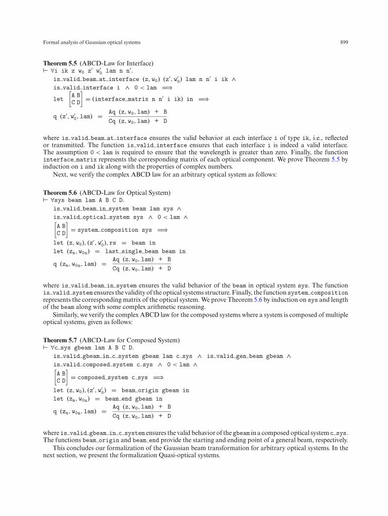
In order to ensure the correctness of our definitions and to facilitate the formal analysis of practical systems,we verify three classical results of Gaussian beams theory: (1) ABCD-law for each optical interface (i.e., freespace, spherical and plane for both reflection and transmission); (2) ABCD-law for an arbitrary optical system;and (3) for composed optical systems as follows:


Theorem 5.5 (ABCD-Law for Interface)� ∀i ik z w0 z′ w′

0 lam n n′.is valid beam at interface (z, w0) (z′, w′

0) lam n n′ i ik ∧is valid interface i ∧ 0 < lam �⇒let

[A BC D

]� (interface matrix n n′ i ik) in �⇒

q (z′, w′0, lam) � Aq (z, w0, lam) + B

Cq (z, w0, lam) + D

where is valid beam at interface ensures the valid behavior at each interface i of type ik, i.e., reflectedor transmitted. The function is valid interface ensures that each interface i is indeed a valid interface.The assumption 0 < lam is required to ensure that the wavelength is greater than zero. Finally, the functioninterface matrix represents the corresponding matrix of each optical component. We prove Theorem 5.5 byinduction on i and ik along with the properties of complex numbers.

Next, we verify the complex ABCD law for an arbitrary optical system as follows:

Theorem 5.6 (ABCD-Law for Optical System)� ∀sys beam lam A B C D.

is valid beam in system beam lam sys ∧is valid optical system sys ∧ 0 < lam ∧[A BC D

]� system composition sys �⇒

let (z, w0), (z′, w′0), rs � beam in

let (zn, w0n) � last single beam beam in

q (zn, w0n, lam) � Aq (z, w0, lam) + B

Cq (z, w0, lam) + D

where is valid beam in system ensures the valid behavior of the beam in optical system sys. The functionis valid system ensures the validity of the optical systems structure. Finally, the functionsystem compositionrepresents the corresponding matrix of the optical system.We prove Theorem 5.6 by induction on sys and lengthof the beam along with some complex arithmetic reasoning.

Similarly, we verify the complex ABCD law for the composed systems where a system is composed of multipleoptical systems, given as follows:

Theorem 5.7 (ABCD-Law for Composed System)� ∀c sys gbeam lam A B C D.

is valid gbeam in c system gbeam lam c sys ∧ is valid gen beam gbeam ∧is valid composed system c sys ∧ 0 < lam ∧[A BC D

]� composed system c sys �⇒

let (z, w0), (z′, w′0) � beam origin gbeam in

let (zn, w0n) � beam end gbeam in


Cq (z, w0, lam) + D

where is valid gbeam in c system ensures the valid behavior of the gbeam in a composed optical system c sys.The functions beam origin and beam end provide the starting and ending point of a general beam, respectively.

This concludes our formalization of the Gaussian beam transformation for arbitrary optical systems. In thenext section, we present the formalization Quasi-optical systems.


Fig. 8. Quasi-optical system design flow [Gol98]

Table 2. Beam waist criticality of different quasi-optical components [Gol98]

Nature of criticality Optical component

Non-critical PolarizationModerately critical Diffraction grating, Plate filters, Dielectric filled Fabry Perot resonatorHighly critical Beam interferometer, Fabry Perot interferometerDetermined by components Resonators, Feed horn

6. Formal analysis of quasi-optical systems

Given the quasi-optical system design and performance specification, i.e., the information about the size of theoverall system, operating frequencies and coupling requirements, we can break the design procedure into foursteps as shown in Fig. 8.

• Determination of the system architecture and quasi-optical components: The system architecture means thearrangement of optical components (lenses or mirrors), their nature (i.e., reflective or transmissive) and theability to process frequency bands. In industrial settings, this initial decision is of central importance becausethe choice of the components can only be considered correct after executing all the steps mentioned in Fig. 8.

• Beam waist radius: The beam waist radius provides a suitable measure to evaluate how each componentmodifies the Gaussian beam. In practice, there are many useful quasi-optical components for which beamwaist radius is not important from an application viewpoint (e.g., polarization rotators, which rotate thepolarization axis of the light beams [Gol98]). So one of the most important design criteria is the identificationof all the components in a system for which the beamwaist radius is critical. A summary of such quasi-opticalcomponents along with their criticality is described in Table 2.

• Beam waist location: The coupling of a Gaussian beam among two optical components is critical to increasethe overall performance of systems such as laser resonators [ST07] and feed-horns [Gol98]. This can be doneby the identification of the beam waist location along with the beam waist radius of Gaussian beams at theinput and output of each quasi-optical component.

• Evaluation and verification: Finally, the last step is to evaluate and verify that the selected architecture of thequasi-optical system meets the performance specification, i.e., Gaussian beam waist radius and location aresuitable for the correct operation. Moreover, in some practical situations it is compulsory to evaluate themagnification, which is a ratio of the minimum beam waists of input and output Gaussian beams.


Fig. 9. Generalized quasi-optical system

In order to perform the verification and evaluation (Fig. 8) of quasi-optical systems, we formally derive theexpressions for the beam waist radius and location of the output Gaussian beam in the following section.

6.1. Gaussian beam transformation by a generalized quasi-optical system

The generalized properties of beam transformation through a quasi-optical system can be analyzed using theABCD-law as described in Sect. 5.3. We consider a generic case in which a quasi-optical system is modeled asan arbitrary ABCD-matrix as shown in Fig. 9. The input waist radius w0in of the Gaussian beam is located atdistance din from the input reference plane, and the output waist radius w0out , is located at distance dout fromthe output reference plane. In this situation, the whole system is composed of three subsystems, i.e., a free space(ni , din ), a quasi-optical system (which we model as an ABCD-matrix), and another free space, i.e., (n0, dout ).Our main goal is to derive the generic expression for the beam waist radius and its location as these are the twocritical requirements in the design and analysis of quasi-optical systems. To this aim, we require three steps: (1)building a formal model of the quasi-optical system described in Fig. 9 and then verifying the equivalent matrix;(2) deriving the ABCD-law using the system equivalent matrix; and (3) deriving the general expressions for theoutput beam width radius and its location, i.e., w0out and dout , respectively. We formally model the quasi-opticalsystem described in Fig. 9 as follows:

Definition 6.1 (Quasi-Optical System Model)� ∀ni din sys n0 dout.

quasi optical system sys din dout ni n0 � [[ ], ni, din; sys; [ ], n0, dout]

where sys represents the quasi-optical system, the parameters ni and n0 represent the refractive index at theinput and output, respectively. We next verify the equivalent matrix relation when the system is represented as anarbitrary ABCD-matrix as follows:

Theorem 6.1 (Matrix of Quasi-Optical System)� ∀sys din dout ni n0 A B C D.

system composition sys �[A BC D

]�⇒

composed system (quasi optical system sys din dout ni n0) �[A + Cdout Adin + B + Cdindout + Dddout

C Cdin + D

]


The proof of this theorem involves rewriting the definitions of quasi optical system and composed systemalong with the corresponding matrices of the input and output free spaces.

Consequently, we verify the ABCD-law for the quasi-optical system model (Definition 6.1) as follows:

Theorem 6.2 (Quasi-optical System (ABCD))� ∀sys din dout ni n0 gbeam lam A B C D.

is valid gbeam in c system gbeam lam (quasi optical system sys din dout ni n0) ∧is valid gen beam gbeam ∧is valid composed system (quasi optical system sys din dout ni n0) ∧ 0 < lam ∧[A BC D

]� system composition sys �⇒

let (z, w0), (z′, w′0) � beam origin gbeam in

let (zn, w0n) � beam end gbeam in


Cq (z, w0, lam) + D

where the first assumption ensures the valid behavior of the beam when it propagates through the quasi-opticalsystem. The proof of this theorem is a direct consequence of Theorem 5.7.

Our next step is to verify the general expressions for the output beam waist radius. Here, one important pointis to ensure that we are only interested in the Gaussian beam waist at the input, which means that the real part ofthe input q-parameter should be 0.We include this requirement in the verification of the following main theorem:

Theorem 6.3 (Beam Waist Radius and Location)� ∀sys gbeam din dout lam ni n0 w0in w0out z zn A B C D.

[H1] sys constraints (quasi optical system sys din dout ni n0) ∧[H2]

[A BC D

]� system composition sys ∧

[H3] (z, w0in) � beam origin gbeam ∧ (zn, w0out) � beam end gbeam ∧[H4] Re(q (z, w0in, lam)) � 0 ∧ Re(q (zn, w0out, lam)) � 0 ∧

(Cdin + D)2 + (C rayleigh range w0in lam)2 �� 0 �⇒dout � − (Adin + B)(Cdin + D) + AC(rayleigh range w0in lam)2

(Cdin + D)2 + (C(rayleigh range w0in lam)2)∧

w0out2 � (AD − BC) w0in

2

(Cdin + D)2 + (Cw0in2π

lam)2

where the first assumption [H1] packages three conditions as system constraints, i.e., the validity of the composedoptical systemarchitecture, the validityof a general beamand thevalidbehaviorof a general beam in the composedsystem. The second assumption [H2] ensures that the composed system can be described by an arbitrary matrix.Finally, the third and fourth assumptions (i.e., [H3] and [H4]) ensure that the real part of q-parameters are zeroand the values dout and w0out are finite. The proof of Theorem 6.3 is mainly based on Theorem 6.2 and involvesthe properties of complex numbers (mainly, equating the real and imaginary parts of the input and outputq-parameters).

Note that the expressions obtained in Theorem 6.3 can be applied to any quasi-optical system and Gaussianbeamparameters. The given system itself can be arbitrarily complicated, and the analysis is reduced to the problemof obtaining its overall ABCD-matrix from a cascaded representation of its constituent optical components. Weapply these results to verify a real-world optical system in the next section.


Fig. 10. Optical layout of the APEX telescope facility receiver [NLD+09]

6.2. Optics verification of Atacama pathfinder experiment (APEX) telescope receiver

The Atacama Pathfinder EXperiment (APEX)3 is a single dish (12-m diameter) telescope for millimeter and sub-millimeter astronomy, which has been in operation since its inauguration in 2005 [NLD+09]. The main missionof the APEX is to conduct the astronomical study of cold dust and gas in our own milky way and in distantgalaxies. Recent observations based onAPEX reveal the cradles ofmassive star-formation throughout our galaxy[APE15]. In addition to these interesting aspects of the APEX telescope, the other main function is radiometrywhich helps to provide reliable weather forecasts and environmental dynamics. One of the main modules of theAPEX is the SwedishHeterodyne Facility Instrument (SHeFI) receiver whichwas installed in 2008. In [NLD+09],the authors used a Quasi-optics-based model for the SHeFI receiver to derive the conditions in terms of beamparameters using a paper-and-pencil based proof approach. Furthermore, these constraints are used to optimize(i.e., minimization of dimensions and distortions) the telescope design for all optical components. In this thesis, wepropose to formally analyze the SHeFI receiver within the sound core of HOL Light by using our formalizationof Gaussian beams and quasi-optical systems. The main component of the SHeFI receiver is the optical system,which is designed to provide the coupling of the SHeFI channels and other instruments within the telescope. Theoptical layout of the receiving cabin is shown in Fig. 10. The pointsO1,O2, andO3 represent focal points, tracedfrom the original Cassegrain focal point [NLD+09]. Here,M8s andM10 are ellipsoidalmirrors with focal distancesf2 and f1 [NLD+09], respectively. In this situation, the Gaussian beams’ transformation is the best possible wayto understand the processing of light in the receiver module of the APEX telescope [NLD+09].

Our main goal is to verify a generic expression for the system magnification, which is represented by the ratioof output and input beam waist radii, i.e.,

w0out

w0in. This can be done by using already verified theorems in our

framework. We analyze one module of the receiving system, i.e., the gray shaded region in Fig. 10. Indeed, thiscan be considered as the quasi-optical system with the input and output distances L1 and L2 and a thin lensinside. Our problem is mainly reduced to the derivation of the equivalent matrix relation for the thin lens andthen utilize Theorems 6.2 and 6.3. A thin lens is represented as the composition of two transmitting sphericalinterfaces such that any variation of the beam parameters is neglected between both interfaces. So, at the end, athin lens is the composition of two spherical interfaces with a null width free space in between. We formalize athin lens as follows:

Definition 6.2 (Thin Lens)� ∀R1 R2 n0 n1. thin lens R1 R2 n0 n1 =

([(n0,0),spherical R1,transmitted; (n1,0),spherical R2,transmitted],(n0,0))

where R1, R2, n1, n2, represent the radius of curvatures of two interfaces and the refractive indices of the inputand output planes, respectively. We prove that a thin lens is indeed a valid optical system if the correspondingparameters satisfy some constraints:

3 http://www.apex-telescope.org/.



Theorem 6.4 (Valid Thin Lens)� ∀R1 R2 n0 n1. R1 �� 0 ∧ R2 �� 0 ∧ 0 < n0 ∧ 0 < n1 �⇒

is valid optical system (thin lens R1 R2 n0 n1)

The proof of this theorem is done automatically by our developed tactic, called VALID OPTICAL SYSTEM TAC.Next, we verify the matrix relation of the thin lens as follows:

Theorem 6.5 (Thin Lens Matrix)� ∀R1 R2 n0 n1. R1 �� 0 ∧ R2 �� 0 ∧ 0 < n0 ∧ 0 < n1 �⇒

system composition (thin lens R1 R2 n0 n1) =

[1 0

n1 − n0n0

(1

R2− 1

R1) 1

]

At this point, we have all the necessary ingredients to analyze the module of interest of the SHeFI receiveras shown in Fig. 10. We reuse the definition of the generalized quasi-optical system (Definition 6.1) to define themodule as follows:

Definition 6.3 (SheFI Receiver Module)� ∀R1 R2 L1 L2 n1 n2.

SHeFI receiver model L1 L2 n1 n2 R1 R2 �quasi optical system (thin lens R1 R2 n1 n2) L1 L2 n1 n2

Finally, we verify the system magnification of the SheFI receiver module as follows:

Theorem 6.6 (APEX Beam Waist)� ∀gbeam L1 L2 lam n1 n2 R1 R2.

SHeFI constraints gbeam L1 L2 lam n1 n2 R1 R2 �⇒let f � − 1(

n2 − n1n1

1

R2− 1

R1

) and

(z, w0) � beam origin gbeam and

(zn, w0n) � beam end gbeam in

(1 − L11

f)2 + (

1

f(rayleigh range w0in lam))2 �� 0 �⇒

w0out2

w0in2� 1(

1 − L11

f

)2

+(1

f(rayleigh range w0in lam)

)2

We verify the above expression using Theorems 6.5 and 6.3. Note that Theorem 6.6 is in a general form and canfurther be utilized to reason about different cases such as the input and output distances (L1 and L2) are equalto f , or 2f , in order to maximize or minimize the magnification depending upon the practical requirements. Wecan easily evaluate the real values of the parameters provided by physicists and optical engineers. Indeed, theonly requirement is to check SHeFI constraints, which ensures the valid behavior of gbeam in thin lens-basedquasi-optical systems.

This completes the formal analysis of the quasi-optical systems based on the Gaussian beam transforma-tion. Due to the generic nature of our models and verified theorems, we have been able to analyze a cost andsafety critical application, i.e., the receiver module of the APEX telescope within the sound core of HOLLight theorem prover. This improved accuracy comes at the cost of the time and effort spent, formalizing


the underlying theories of ray optics andGaussian beams. But, the availability of such a formalized infrastructuresignificantly reduces the time required to analyze the quasi-optical systems and the APEX telescope application.For example, the analysis of the application, i.e., the modeling and verification of the systemmagnification of thereceiver module took less than 100 lines of HOL light code and a couple of hours by an expert user of HOLLight.Apart from the formalization of a number of concepts of ray optics and Gaussian optics, another contribution ofour work is to bring out all the hidden assumptions about the physical models of ray, beams, lenses and mirrors,which otherwise are not mentioned in the optics literature (e.g., [Tra07]). Moreover, we automatized parts of theverification task by introducing new tactics. Some of these tactics are specialized to verify (or simplify) the proofsrelated to our formalization of optical systems (e.g., VALID OPTICAL SYSTEM TAC). However, some tactics aregeneral and can be used in different verification tasks involving matrix/vector operations. An example of such atactic is common prove, which allowed us to verify the ray-transfer matrices in our development. The automationof proof tasks is mainly done using the derived rules and tactics of HOL Light, so that the application to aparticular system does not involve the painful manual proofs often required with interactive (higher-order logic)theorem proving.

7. Conclusion and future work

In this paper, we reported a new engineering application of formal methods in the area of Gaussian opticalsystems. In particular, we proposed to use higher-order-logic theorem proving as a complementary technique toverify some important properties of real-world optical systems. We also presented the formalization of Gaussianbeams based on the notion of q-parameters along with the verification of ABCD-law for arbitrarily composedoptical systems. Building on top of this infrastructure, we analyzed a cost and safety critical application, i.e.,the receiving unit of the Atacama Pathfinder Experiment (APEX) telescope. The analysis accuracy of theoremproving allowed us to unveil all the assumptions required to verify the magnification of the SHeFI receiver.

The formal analysis of Gaussian optical systems along with the real-world critical applications (e.g., APEXtelescope) provides some thoughtful indications: (1) Theorem proving systems have reached maturity, wherecomplex physical models can be expressed with less effort than ever before; and (2) Formal methods can assistin the verification of futuristic optical systems, which are largely becoming parts of critical applications suchas military setups, biomedical surgeries and space missions. However, the question of the utilization of higher-order-logic theorem proving in industrial settings (particularly, physical systems) still persists due to the hugeamount of time required to formalize the underlying theories. We believe that an important factor is the gapbetween theorem proving and engineering communities, which limits its usage in industrial settings. For example,it is hard to find engineers (or physicists) with a theorem proving background and vice-versa. One of the severalsolutions to tackle this issue is the continuous formal development of optics theories including the libraries ofthe most frequently used optical components and devices, which can ultimately reduce the cost of using formalmethods (particularly theorem proving) as an integral part of the design and verification of physical systems.The work reported in this paper can be considered as a step towards this goal with more efforts to follow inthe same or closely related disciplines such as quantum optics, photonic signal processing and optoelectronics.Our plan is to extend this work in order to obtain an extensive library of verified optical components such asphase-conjugate mirrors and resonators with active sources inside [HW05a], which would allow a practical useof our formalization in industry. We also intend to formalize and verify the correctness and soundness of the rayand Gaussian beam tracing algorithms [Tra07], which are included in almost all optical systems design tools.

The formal analysis of real-world systems involves mathematical models which usually represent an ap-proximated behavior of physical phenomena. In order to formally treat the approximations introduced in phys-ical models, we need to consider non-standard analysis and asymptotic notations. For example, small angleapproximation (or paraxial approximation) entails that sin(θ ) ≈ θ , and it can be treated using asymptoticnotations. Interestingly, both non-standard analysis [Fle01] and asymptotic notations [AD04] are available inIsabelle/HOL.4 Our work can be extended by using these concepts which will bring more rigor to the for-mal models of optical systems. Similar concepts can also be used to formally prove that ray optics models areapproximations of wave and electromagnetic optics models. Recently, a learning-assisted automated reasoning

4 http://isabelle.in.tum.de.

http://isabelle.in.tum.de


support [KU14] has been developed for HOL Light, which can also be applied in our formalization to see thefuture of automation tools for optics and the formalization of Physics [KUS+15]. Moreover, our formalizationcan be adapted to other widely used theorem provers (e.g., PVS5 and Isabelle/HOL), which provide efficientautomation support. In the future, it might be possible to automatically port our formalization to other theoremprovers with the maturity of some ongoing projects like the Open Theory Project6 and ProofPeer.7

References

[AD04] Avigad J, Donnelly K (2004) Formalizing O notation in Isabelle/HOL. In: Automated reasoning, Lecture Notes in ComputerScience, vol 3097. Springer, Berlin, Heidelberg, pp 357–371

[APE15] Atacama Pathfinder EXperiment (APEX) (2015) http://www.apex-telescope.org/[ASM+14] Afshar SK, Siddique U, Mahmoud MY, Aravantinos V, Seddiki O, Hasan O, Tahar S (2014) Formal analysis of optical

systems. Math Comput Sci 8(1):39–70[CSBE10] Chabory A, Sokoloff J, Bolioli S, Elis K (2010) Application of gaussian beam based techniques to the quasi-optical systems

of radiofrequency radiometers. In: European Conference on Antennas and Propagation, vol 2010, pp 12–16[Dam05] Damask JN (2005) Polarization optics in telecommunications. Springer Series in Optical Sciences. Springer[FAGP13] Franke-Arnold S, Gay SJ, Puthoor IV (2013) Quantum process calculus for linear optical quantum computing. In: Reversible

Computation, Lecture Notes in Computer Science, vol 7948. Springer, pp 234–246[Fle01] Fleuriot JD (2001)Nonstandard geometric proofs. In: Automated deduction in geometry, LectureNotes inComputer Science,

vol 2061. Springer, pp 246–267[Gol98] Goldsmith PF (1998) Quasioptical systems: gaussian beam quasioptical propogation and applications. IEEE Press Series on

RF and Microwave Technology. Wiley[Gri05] Griffiths DJ (2005) Introduction to quantum mechanics. Pearson Prentice Hall[Har09a] Harrison J (2009) Handbook of practical logic and automated reasoning. Cambridge University Press[Har09b] Harrison J (2009) HOL light: an overview. In: Theorem Proving in Higher Order Logics, Lecture Notes in Computer Science,

vol 5674. Springer, pages 60–66[Har13] Harrison J (2013) The light theory of Euclidean space. J Autom Reason. 50(2):173–190[HW05a] Hodgson N, Weber H (2005) Optical resonators: fundamentals, advanced concepts, applications. Springer Series in Optical

Sciences. Springer[HW05b] Hodgson N, Weber H (2005) Optical resonators: fundamentals, advanced concepts, applications. Springer[KAHT14] Khan-Afshar S, Hasan O, Tahar S (2014) Formal analysis of electromagnetic optics. In: Novel optical systems design and

optimization, SPIE, vol 9193, pp 91930A–91930A–14[KL66] Kogelnik H, Li T (1966) Laser beams and resonators. Appl Opt. 5(10):1550–1567[KU14] Kaliszyk C, Urban J (2014) Learning-assisted automated reasoning with flyspeck. J Autom Reason. 53(2):173–213[KUS+15] Kaliszyk C, Urban J, Siddique U, Khan-Afshar S, Dunchev C, Tahar S (2015) Formalizing physics: automation, presentation

and foundation issues. In: Intelligent computer mathematics, Lecture Notes in Computer Science, vol 9150. Springer, pp288–295

[LAS15] LASCAD (2015) http://www.las-cad.com/[Moo01] Mookherjea S(2001) Analysis of optical pulse propagation with two-by-two (ABCD) matrices. Phys Rev E. 64(016611):1–10[MPM+11] MalakM, PavyN,Marty F, Peter Y, Liu AQ, Bourouina T (2011) Stable, high-Q fabry-perot resonators with long cavity based

on curved, all-silicon, high reflectance mirrors. In: IEEE international conference on micro electro mechanical systems, pp720–723

[MT14] Mahmoud MY, Tahar S (2014) On the quantum formalization of coherent light in HOL. In: NASA formal methods, LNCS,vol 8430. Springer, pp 128–142

[NKST98] NakazawaM, Kubota H, Sahara A, Tamura K (1998) Time-domain ABCDMatrix Formalism for Laser Mode-Locking andOptical Pulse Transmission. IEEE J Quantum Electron 34(7):1075–1081

[NLD+09] Nystrm O, Lapkin I, Desmaris V, Dochev D, Ferm S-E, FredrixonM, Henke D, Meledin D, Monje R, StrandbergM, SundinE, Vassilev V, Belitsky V (2009) Optics design and verification for the APEX Swedish heterodyne facility instrument (SHeFI).J Infrared Millim Terahertz Waves. 30(7):746–761

[Opt15] Optica (2015) http://www.opticasoftware.com/[reZ15] reZonator (2015) http://www.rezonator.orion-project.org/[SAT13a] Siddique U, Aravantinos V, Tahar S (2013) Formal stability analysis of optical resonators. In: NASA formal methods, Lecture

Notes in Computer Science, vol 7871, pp 368–382[SAT13b] Siddique U, Aravantinos V, Tahar S (2013) On the formal analysis of geometrical optics in HOL. In: Automated deduction in

geometry, Lecture Notes in Computer Science, vol 7993, pp 161–180[Sid15] Siddique U (2015) Formal analysis of gaussian optical systems: source code. http://hvg.ece.concordia.ca/projects/optics/

gaussian.html

5 http://pvs.csl.sri.com.6 http://www.gilith.com/research/opentheory/.7 http://www.proofpeer.net.


http://www.las-cad.com/

http://www.opticasoftware.com/

http://www.rezonator.orion-project.org/

http://hvg.ece.concordia.ca/projects/optics/gaussian.html

http://hvg.ece.concordia.ca/projects/optics/gaussian.html

http://pvs.csl.sri.com

http://www.gilith.com/research/opentheory/

http://www.proofpeer.net


[ST07] Saleh BEA, Teich MC (2007) Fundamentals of photonics. Wiley[SXS+11] Su B, Xue J, Sun L, Zhao H, Pei X (2011) Generalised ABCD matrix treatment for laser resonators and beam propagation.

Opt Laser Technol 43(7):1318–1320[SZL+06] Song WZ, Zhang XM, Liu AQ, Lim CS, Yap PH, Hosseini HMM (2006) Refractive index measurement of single living cells

using on-chip Fabry-Perot cavity. Appl Phys Lett 89(20):203901[Tra07] Trager F (2007) Handbook of lasers and optics. Springer.[WA05] WilsonWC,AtkinsonGM (2005)MOEMSmodeling using the geometrical matrix toolbox. Technical report, NASA, Langley

Research Center[Wel91] Wellner M (1991) Wave optics. In: Elements of physics, pp 543–575. Springer

Received 28 May 2015Accepted in revised form 15 February 2016 by Stephan Merz, Jun Pang, and Jin Song DongPublished online 15 March 2016

Documents

On the formal analysis of Gaussian optical systems in HOLhvg.ece.concordia.ca/Publications/Journals/FAC16.pdfOn the formal analysis of Gaussian optical systems in HOL Umair Siddique1