On the generalized low rank approximation of the correlation matrices arising in the asset portfolio

Linear Algebra and its Applications 461 (2014) 1–17

Contents lists available at ScienceDirect

Linear Algebra and its Applications

www.elsevier.com/locate/laa

On the generalized low rank approximation of the

correlation matrices arising in the asset portfolio ✩

Xuefeng Duan ∗, Jianchao Bai, Maojun Zhang, Xinjun ZhangCollege of Mathematics and Computational Science, Guilin University of Electronic Technology, Guilin 541004, PR China

a r t i c l e i n f o a b s t r a c t

Article history:Received 12 October 2013Accepted 21 July 2014Available online xxxxSubmitted by R. Brualdi

MSC:11D0768W2565F30

Keywords:Generalized low rank approximationCorrelation matrixAsset portfolioFeasible setConjugate gradient algorithm

In this paper, we consider the generalized low rank approxima-tion of the correlation matrices problem which arises in the asset portfolio. We first characterize the feasible set by using the Gramian representation together with a special trigonometric function transform, and then transform the generalized low rank approximation of the correlation matrices problem into an unconstrained optimization problem. Finally, we use the conjugate gradient algorithm with the strong Wolfe line search to solve the unconstrained optimization problem. Numerical examples show that our new method is feasible and effective.

Published by Elsevier Inc.

✩ The work was supported by National Natural Science Foundation of China (Nos. 11101100; 11261014; 11301107; 61362021), Natural Science Foundation of Guangxi Province (No. 2012GXNSFBA053006; 2013GXNSFBA019009; 2013GXNSFBB053005; 2013GXNSFDA019030), the Fund for Guangxi Experiment Center of Information Science (20130103), Innovation Project of GUET Graduate Education (GDYCSZ201473), Innovation Project of Guangxi Graduate Education (YCSZ2014137), and Guangxi Key Lab of Wireless Wideband Communication and Signal Processing open grant 2012.* Corresponding author.

E-mail addresses: [email protected] (X. Duan), [email protected] (J. Bai).

http://dx.doi.org/10.1016/j.laa.2014.07.0260024-3795/Published by Elsevier Inc.

http://dx.doi.org/10.1016/j.laa.2014.07.026

http://www.ScienceDirect.com/

http://www.elsevier.com/locate/laa

mailto:[email protected]

mailto:[email protected]

http://dx.doi.org/10.1016/j.laa.2014.07.026

http://crossmark.crossref.org/dialog/?doi=10.1016/j.laa.2014.07.026&domain=pdf

2 X. Duan et al. / Linear Algebra and its Applications 461 (2014) 1–17

1. Introduction

Throughout this paper, we use Rn×n and S+n to denote the set of n × n real matrices

and symmetric positive semidefinite matrices, respectively. We use AT and tr(A) to represent the transpose and trace of the matrix A, respectively. The symbols ‖A‖F and rank(A) denote the Frobenius norm and the rank of the matrix A, respectively. The symbol diag(Y ) stands for the vector whose elements lie in the diagonal line of the matrix Y , and the symbol e stands for the vector whose elements are of all ones, i.e., e = (1, 1, · · · , 1)T .

In this paper, we consider the following problem named generalized low rank approx-imation of the correlation matrices.

Problem 1.1. Given some correlation matrices A(d) ∈ Rn×n, d = 1, 2, · · · , m, and a positive integer k, 1 ≤ k < n, find a correlation matrix Y whose rank is less than and equal to k such that

12

m∑d=1

∥∥A(d) − Y∥∥2F

= minY ∈S+

n , diag(Y )=e, rank(Y )≤k

12

m∑d=1

∥∥A(d) − Y∥∥2F. (1.1)

Problem (1.1) arises in the asset portfolio (see [10] for more details), which can be stated as follows. Suppose that R = DCD is the covariance matrix of n assets, where C is a correlation matrix and D is a diagonal matrix with positive variances which are specially used to describe the risk of assets. In practice, the covariance matrix is usually estimated by the historical data of the return of each asset, that is, an approximation covariance is obtained by statistics method. Let

R(d) = D(d)C(d)D(d)

be the approximation covariance with dth sampling some data, where D(d) and C(d)

are the dth approximation diagonal matrix and correlation matrix, respectively. Higham [4] proposed a method for finding the nearest low rank approximation of a correlation matrix by only one sampling (i.e., m = 1). However, it is difficult for the decision maker to choose the best approximation covariance matrix with only one sampling because there is always a noise in the data on the prices of assets. Thus, we develop a repeated sampling method to get a series of approximation covariance matrices, that is, d comes from 1 to m. Obviously, it is very easy to obtain the optimal diagonal matrix D by a series of D(d). The major obstacle to finding the optimal covariance matrix is conducting the optimal correlation matrix C from a series of C(d). The above consideration leads to solving the following problem: given some correlation matrices A(1), A(2), · · · , A(m) ∈ Rn×n, find a correlation matrix Y such that

12

m∑∥∥A(d) − Y∥∥2F

= minY ∈S+

n , diag(Y )=e

12

m∑∥∥A(d) − Y∥∥2F. (1.2)

d=1 d=1

X. Duan et al. / Linear Algebra and its Applications 461 (2014) 1–17 3

Meanwhile, for the large financial correlation matrices, usually almost all variances can be attributed to some stochastic Brownian factors. Therefore, instead of taking into account all Brownian motions, we would wish to simulate with a smaller number of factors, i.e., rank(Y ) < n and typically rank(Y ) is from 1 to k. Then the problem (1.2)with rank constraint becomes problem (1.1).

Noting that the matrix Y in problem (1.1) is not only positive semidefinite but also satisfies rank(Y ) ≤ k, so problem (1.1) belongs to the structured low rank approximation problem. As Gillard–Zhigljavsky [3] said, the structured low rank approximation is a difficult optimization problem, so there is much work to be done. In the last few years, there has been a constantly increasing interest in developing the theory and numerical methods for the nearest low rank approximation of a correlation matrix, due to their wide applications in the fiance and risk management [6], machine learning [15], stress testing of bank [13], industrial process monitoring [7] and image processing [5]. Recently, problem (1.1) with m = 1 has been extensively studied, and the research results mainly concentrate on the following two cases. One is without the rank constraint and the other is with the rank constraint.

For the case without the rank constraint, Higham [4] proposed an alternative projec-tion algorithm to solve the nearest correlation matrix problem by defining two projection operators. Under some proper assumptions, Li–Li [8] developed a projected semismooth Newton method to solve the problem of calibrating least squares covariance matrix. Qi and Sun [12] proposed a Newton-type method for the nearest correlation matrix prob-lem, and the quadratic convergence of the new method was proved. An unconstrained convex optimization approach was proposed to find the nearest correlation matrix to the target matrix with the fixed correlations unaltered in Ref. [13]. Besides, Qi–Sun [14]constructed an augmented Lagrangian dual method for the H-weighted nearest correla-tion matrix problem. This method solves a sequence of unconstrained strongly convex optimization problems, each of which can be solved by a semismooth Newton method combined with the conjugate gradient method. Recently, Yin, et al. [18,20] developed two new alternative gradient algorithms to compute the nearest correlation matrix by making use of the alternative gradient method.

For the case with the rank constraint, by making use of the fact that

Y ∈ S+n , rank(Y ) ≤ k ⇐⇒ λk+1(Y ) + · · · + λn(Y ) = 0,

Gao and Sun [2] proposed a majorized penalty approach for solving the rank constrained correlation matrix problem. It is noted that Gao and Sun’s majorized penalty approach can deal with some large scale problems (n ≥ 500). Motivated by the method in [12]and based on a well-known result that the sum of the largest eigenvalues of a symmetric matrix can be represented as a semidefinite programming problem, Li–Qi [9] proposed a novel sequential semismooth Newton method to solve problem (1.1) with m = 1. They formulate the problem as a bi-affine semidefinite programming and then use an augmented Lagrange method to solve a sequence of least squares problems. Both Simon–


Abell [16] and Pietersz–Groenen [11] used majorization approach to solve the low rank approximation of a correlation matrix. The difference lies in that the former solved the problem with any weighted norm while the latter only settled it with Frobenius norm. By constructing a Lagrange function, Zhang–Wu [21] transformed the low rank approx-imation of a correlation matrix into a min–max problem, where the inner maximization problem was solved with closed form spectral decomposition and the outer minimiza-tion problem was solved with gradient-based methods. In [1], Grubisic and Pietersz introduced a geometric programming approach to solve the low rank nearest correlation matrix problem. The method could be used to minimize any sufficiently smooth objective function.

However, the research results of problem (1.1) with m > 1 are very few as far as we know. The greatest difficulties to solve problem (1.1) are how to characterize the feasible set and deal with the complex structure. In this paper, we overcome these difficulties by using the Gramian representation together with a special trigonometric function trans-form. Then problem (1.1) is transformed into an unconstrained optimization problem. Finally, the conjugate gradient method with the strong Wolfe line search is given to solve the unconstrained optimization problem. Numerical examples show that our new method is feasible and effective.

2. Main results

In this section, we first transform problem (1.1) into an unconstrained optimization problem by making use of the Gramian representation together with a special trigono-metric function transform. Then we use the conjugate gradient algorithm with the strong Wolfe line search to solve it.

We first define the following set

S ={Y ∈ Rn×n

∣∣ Y ∈ S+n , rank(Y ) ≤ k

}.

It is easy to characterize the set S by using the Gramian representation (see [17]), i.e.,

Y = XXT , X ∈ Rn×k.

Set

Γ ={Y ∈ Rn×n

∣∣ diag(Y ) = e}.

It is easy to verify that the feasible set of problem (1.1) is S ∩ Γ . The most difficulty to solve problem (1.1) is how to characterize the feasible set. Now we begin to use the Gramian representation together with a special trigonometric function transform to characterize the feasible set S ∩ Γ .


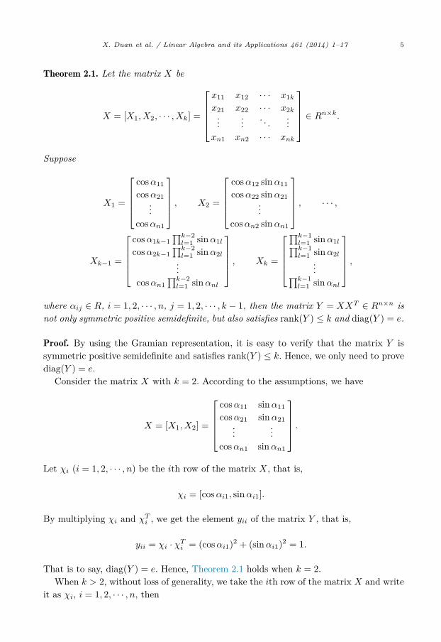
Theorem 2.1. Let the matrix X be

X = [X1, X2, · · · , Xk] =

⎡⎢⎢⎢⎣x11 x12 · · · x1kx21 x22 · · · x2k...

.... . .

...xn1 xn2 · · · xnk

⎤⎥⎥⎥⎦ ∈ Rn×k.

Suppose

X1 =

⎡⎢⎢⎢⎣cosα11cosα21

...cosαn1

⎤⎥⎥⎥⎦ , X2 =

⎡⎢⎢⎢⎣cosα12 sinα11cosα22 sinα21

...cosαn2 sinαn1

⎤⎥⎥⎥⎦ , · · · ,

Xk−1 =

⎡⎢⎢⎢⎣cosα1k−1

∏k−2l=1 sinα1l

cosα2k−1∏k−2

l=1 sinα2l...

cosαn1∏k−2

l=1 sinαnl

⎤⎥⎥⎥⎦ , Xk =

⎡⎢⎢⎢⎣∏k−1

l=1 sinα1l∏k−1l=1 sinα2l

...∏k−1l=1 sinαnl

⎤⎥⎥⎥⎦ ,

where αij ∈ R, i = 1, 2, · · · , n, j = 1, 2, · · · , k − 1, then the matrix Y = XXT ∈ Rn×n is not only symmetric positive semidefinite, but also satisfies rank(Y ) ≤ k and diag(Y ) = e.

Proof. By using the Gramian representation, it is easy to verify that the matrix Y is symmetric positive semidefinite and satisfies rank(Y ) ≤ k. Hence, we only need to prove diag(Y ) = e.

Consider the matrix X with k = 2. According to the assumptions, we have

X = [X1, X2] =

⎡⎢⎢⎢⎣cosα11 sinα11cosα21 sinα21

......

cosαn1 sinαn1

⎤⎥⎥⎥⎦ .

Let χi (i = 1, 2, · · · , n) be the ith row of the matrix X, that is,

χi = [cosαi1, sinαi1].

By multiplying χi and χTi , we get the element yii of the matrix Y , that is,

yii = χi · χTi = (cosαi1)2 + (sinαi1)2 = 1.

That is to say, diag(Y ) = e. Hence, Theorem 2.1 holds when k = 2.When k > 2, without loss of generality, we take the ith row of the matrix X and write

it as χi, i = 1, 2, · · · , n, then


χi =[cosαi1, sinαil cosαi2, · · · , cosαik−1

k−2∏l=1

sinαil,

k−1∏l=1

sinαil

].

By multiplying χi and χTi , we get the element yii of the matrix Y , that is,

yii = χi · χTi

= (cosαi1)2 + (sinαil cosαi2)2 + · · · +(

cosαik−1

k−2∏l=1

sinαil

)2

+(

k−1∏l=1

sinαil

)2


k−2∏l=1

sinαil

)2(cos2 αik−1 + sin2 αik−1

)


cosαik−2

k−3∏l=1

sinαil

)2

+(

k−2∏l=1

sinαil

)2


k−3∏l=1

sinαil

)2(cos2 αik−2 + sin2 αik−2

)


cosαik−3

k−4∏l=1

sinαil

)2

+(

k−3∏l=1

sinαil

)2

= · · ·

= (cosαi1)2 + (sinαil cosαi2)2 + (sinαil sinαi2)2

= (cosαi1)2 + (sinαi1)2

= 1.

Hence, for any k ≥ 2, we have yii = 1, i = 1, 2, · · · , n, that is, diag(Y ) = e. �Remark 2.1. As Simon and Abell [16] said, a correlation matrix is a symmetric positive semidefinite matrix with unit diagonal, and any symmetric positive semidefinite matrix with unit diagonal is a correlation matrix. In Theorem 2.1, the matrix Y must be a correlation matrix, and noting that αij, i = 1, 2, · · · , n, j = 1, 2, · · · , k − 1 are arbitrary real number, so the matrix Y = XXT can be represented all the correlation matrices.

Remark 2.2. To explain Theorem 2.1, we take a 3 × 2 matrix for example. Set

X = [X1, X2] =

⎡⎣ cosα11 sinα11cosα21 sinα21cosα31 sinα31

⎤⎦ .


By a simple calculation, we can obtain that

Y = XXT

=

⎡⎣ cosα11 sinα11cosα21 sinα21cosα31 sinα31

⎤⎦⎡⎣ cosα11 sinα11cosα21 sinα21cosα31 sinα31

⎤⎦T

=[ 1 cosα11 cosα21 + sinα11 sinα21 cosα11 cosα31 + sinα11 sinα31

cosα11 cosα21 + sinα11 sinα21 1 cosα21 cosα31 + sinα21 sinα31cosα11 cosα31 + sinα11 sinα31 cosα21 cosα31 + sinα21 sinα31 1

].

Obviously, the matrix Y is not only symmetric positive semidefinite, but also satisfies rank(Y ) ≤ 2 and diag(Y ) = e.

By using the similar way in the proof of Theorem 2.1, we can obtain the other elements of the matrix Y , that is,

Y = (yij)n×n ={∑k−1

p=1 cosαip cosαjp

∏p−1l=1 sinαil sinαjl +

∏k−1l=1 sinαil sinαjl, i = j

1, i = j.

Substituting yij into problem (1.1), it is easy to obtain that problem (1.1) can be written as the following unconstrained optimization problem.

Problem 2.1. Given some correlation matrices A(d) = (A(d)ij )n×n, d = 1, 2, · · · , m, and a

positive integer k, 1 ≤ k < n, find the solution α ∈ Rn×(k−1) of the following optimization problem

minα∈Rn×(k−1)

F (α), (2.1)

where

F (α) =m∑

d=1

n−1∑i=1

n∑j=i+1

(k−1∑p=1

cosαip cosαjp

p−1∏l=1

sinαil sinαjl +k−1∏l=1

sinαil sinαjl −A(d)ij

)2

.

(2.2)

Next, we will use the conjugate gradient algorithm with the strong Wolfe line search to solve the unconstrained optimization problem. The most difficulty to solve problem (2.1) is how to compute the gradient of the objective function F (α). Now we begin to compute the gradient of the objective function.

Theorem 2.2. The gradient of the objective function F (α) of problem (2.1) is

∇F (α) =(∂F (α)∂α11

,∂F (α)∂α21

, · · · , ∂F (α)∂αn1

, · · · , ∂F (α)∂α1k−1

,∂F (α)∂α2k−1

, · · · , ∂F (α)∂αnk−1

)T

,

where


∂F (α)∂αμν

= 2m∑

d=1

n∑i=1, i�=μ

{(k−1∑p=1

cosαμp cosαip

p−1∏l=1

sinαμl sinαil

+k−1∏l=1

sinαμl sinαil −A(d)μi

)

×(− sinαμν cosαiν

ν−1∏l=1

sinαμl sinαil + cosαμν sinαiν

k−1∏l=1, l �=ν

sinαμl sinαil

+ cosαμν sinαiν

k−1∑p=ν+1

cosαμp cosαip

p−1∏l=1, l �=ν

sinαμl sinαil

)}, (2.3)

here μ = 1, 2, · · · , n, ν = 1, 2, · · · , k − 1.

Proof. To prove Theorem 2.2, we only need to prove (2.3) holds when m = 1, because the forms of the expression of the gradient of the objective function F (α) with m = 1are the same as that with m > 1.

For m = 1, noting that the total numbers including αμν in F (α) are

μ−1∑i=1

(k−1∑p=1

cosαμp cosαip

p−1∏l=1

sinαμl sinαil +k−1∏l=1

sinαμl sinαil −Aiμ

)2

+n∑

j=μ+1

(k−1∑p=1

cosαμp cosαjp

p−1∏l=1

sinαμl sinαjl +k−1∏l=1

sinαμl sinαjl −Aμj

)2

.

Hence, the derivative of F (α) at αμν is

∂F (α)∂αμν

= ∂

∂αμν

{μ−1∑i=1

(k−1∑p=1

cosαμp cosαip

p−1∏l=1



)2

+n∑

j=μ+1

(k−1∑p=1

cosαμp cosαjp

p−1∏l=1



)2}

= 2μ−1∑i=1

{(k−1∑p=1

cosαμp cosαip

p−1∏l=1



)


ν−1∏l=1

sinαμl sinαil +k−1∏

l=1, l �=ν

sinαμl sinαil cosαμν sinαiν

+k−1∑

cosαμp cosαip

p−1∏sinαμl sinαil cosαμν sinαiν

)}
p=ν+1 l=1, l �=ν


+ 2n∑

j=μ+1

{(k−1∑p=1

cosαμp cosαjp

p−1∏l=1



)

×(− sinαμν cosαjν

ν−1∏l=1

sinαμl sinαjl +k−1∏

l=1, l �=ν

sinαμl sinαjl cosαμν sinαjν

+k−1∑

p=ν+1cosαμp cosαjp

p−1∏l=1, l �=ν

sinαμl sinαjl cosαμν sinαjν

)}.

Because Aiμ = Aμi, we turn j to i and conclude that

∂F (α)∂αμν

= 2n∑

i=1, i�=μ

{(k−1∑p=1

cosαμp cosαip

p−1∏l=1


sinαμl sinαil −Aμi

)


ν−1∏l=1

sinαμl sinαil + cosαμν sinαiν

k−1∏l=1, l �=ν

sinαμl sinαil

+ cosαμν sinαiν

k−1∑p=ν+1

cosαμp cosαip

p−1∏l=1, l �=ν

sinαμl sinαil

)},

where μ = 1, 2, · · · , n, ν = 1, 2, · · · , k − 1. �Consequently, the conjugate gradient algorithm with the strong Wolfe line search to

solve the minimization problem (2.1) can be described in Algorithm 2.1.

Algorithm 2.1 This algorithm attempts to solve problem (2.1).Step 1. Given parameters ρ ∈ (0, 1), δ ∈ (0, 0.5), σ ∈ (δ, 0.5), and tolerance error 0 ≤ tol � 1. Choose an initial iterative matrix α0 ∈ Rn×(k−1). Set t := 0.Step 2. Calculate gt = ∇F (αt). If ‖ gt ‖F< tol, stop and output α∗ ≈ αt.Step 3. Determine the search direction dt, where

dt ={−gt, t = 0

−gt + gTtgt

gTt−1gt−1

dt−1, t ≥ 1.

Step 4. Confirm the step length βt by applying the strong Wolfe line search, i.e.,

{F (αt+1) ≤ F (αt) + δρmtgT

t dt∣∣gTt+1dt

∣∣ ≤ −σgTt dt.

(2.4)

Set βt = ρmt , γt = αt(:), γt+1 = γt + βtdt, αt+1 = reshape(γt+1, n, k − 1).Step 5. Set t := t + 1. Go to step 2.

Remark 2.3. To implement Algorithm 2.1, we first need to create three matlab files, funfile, gfun file and frac file, where the fun file is used to compute F (αt), the gfun file is used to calculate ∇F (αt), and the frac file is used to minimize F (α). In addition, the


function αt(:) returns the n by k − 1 vector γt whose elements are taken column-wise from the matrix αt, and the function reshape(γt+1, n, k−1) returns the n by k−1 matrix αt+1 whose elements are taken column-wise from γt+1.

By Theorem 4.3.5 [19, p. 203], we can establish the global convergence theorem for Algorithm 2.1.

Theorem 2.3. Suppose the function F (α) is twice continuous and differentiable, the level set

Ω(α0) ={α ∈ Rn×(k−1) ∣∣ F (α) ≤ F (α0)

}is bounded, and the step length βt is generated by (2.4), where δ < σ < 0.5. Then the sequence {αt} generated by Algorithm 2.1 is guaranteed to globally converge, that is,

limt→∞

inf∥∥∇F (αt)

∥∥F

= 0.

3. Numerical experiments

In this section, we use two numerical examples to illustrate that Algorithm 2.1 is feasible to solve problem (2.1). All experiments are tested in Matlab R2010a. We denote the relative residual error

ε(t) =∑m

d=1 ‖A(d) − Yt‖2F∑m

d=1 ‖A(d)‖2F

,

and the gradient norm

‖gt‖F =∥∥∇F (αt)

∥∥F,

where αt is the tth iterative matrix of Algorithm 2.1. We use the stopping criterion

‖gt‖F < 1.0 × 10−4.

And we choose the random matrix rand(m, n) as the initial value in the following exam-ples, where the random matrix is generated by the Matlab function rand(m, n).

Example 3.1. Consider problem (2.1) with m = 1 and

A =

⎡⎢⎢⎣1.0000 0.1849 −0.2867 −0.29970.1849 1.0000 0.2851 0.2582−0.2867 0.2851 1.0000 −0.3100

⎤⎥⎥⎦ .

−0.2997 0.2582 −0.3100 1.0000


Fig. 1. Convergence curves of the relative residual error ε(t) and the gradient norm ‖∇F (αt)‖F .

Case I: Set k = 3. We use Algorithm 2.1 with the initial value

α0 =

⎡⎢⎢⎣0.0344 0.79520.4387 0.18690.3816 0.48980.7655 0.4456

⎤⎥⎥⎦to solve problem (2.1). After 15 iterations, we get the solution α of problem (2.1)

α ≈ α15 =

⎡⎢⎢⎣−1.6439 1.32171.2743 −0.52700.3266 0.81842.2501 0.3043

⎤⎥⎥⎦ .

Hence, the solution Y of problem (1.1) is

Y =

⎡⎢⎢⎣1.0000 0.2403 −0.3495 −0.36190.2403 1.0000 0.3453 0.3179−0.3495 0.3453 1.0000 −0.3777−0.3619 0.3179 −0.3777 1.0000

⎤⎥⎥⎦ .

And the curves of the relative residual error ε(t) and the gradient norm ‖∇F (αt)‖F are in Fig. 1.

Case II: Set k = 2. We use Algorithm 2.1 with the initial value

α0 =

⎡⎢⎢⎣0.95720.48540.80030.1419

⎤⎥⎥⎦to solve problem (2.1). After 13 iterations, we get the solution α of problem (2.1)



Table 1Results for Example 3.1 with different values of rank k.

rank k 2 3Algorithm 2.1 Major 2.1 MajorIT 13 14 15 19CPU (s) 0.0312 0.0624 0.0468 0.1092GN 7.2893 × 10−5 7.7516 × 10−5 7.2330 × 10−5 8.4253 × 10−5

ERR 0.5111 0.5168 0.0092 0.0105

α ≈ α13 =

⎡⎢⎢⎣2.29750.49930.6773−1.0893

⎤⎥⎥⎦ .


Y =

⎡⎢⎢⎣1.0000 −0.2254 −0.0494 −0.9701−0.2254 1.0000 0.9842 −0.0178−0.0494 0.9842 1.0000 −0.1946−0.9701 −0.0178 −0.1946 1.0000

⎤⎥⎥⎦ .


In order to compare our algorithm with the Major algorithm in [11], we use them to solve problem (2.1) with the same initial value. We list the number of iteration (denoted by “IT”), CPU time (denoted by “CPU”), the gradient norm (denoted by “GN”) and the relative residual error (denoted by “ERR”) in Table 1.

Example 3.1 shows that Algorithm 2.1 is feasible to solve problem (1.1). Especially, Table 1 shows that our algorithm outperforms the Major algorithm [11] in both iterations and CPU time, which indicates that our algorithm has faster convergence rate than the Major algorithm.


Next, we will use an example to show that our algorithm can be used to solve the generalized low rank approximation of correlation matrices arising in the asset portfo-lio.

Example 3.2. It is an important issue to calculate the more exact correlation matrix of assets in the portfolio selection. For instance, suppose that an investor uses one unit money to buy a total of 11 assets at the beginning of one period. There is a relation-ship between any two assets of the portfolio because the price of each asset is related to some common factors in the financial market. The correlation matrix is one of the methods measuring the relation between assets. However, how to accurately compute the correlation matrix is the key problem for the investor since the optimal invest-ment policies is affected by the uncertainty of parameters in the correlation matrix. The daily price data of each asset in the portfolio are taken from the Wind database, which is a Chinese financial database, in order to obtain the correlation matrix. Five sets of the daily data are got by the sampling based on five different periods of the data. Using the Matlab software, five correlation matrix of the eleven assets are given as follows.

A(1) =

⎡⎢⎢⎢⎢⎢⎢⎢⎢⎢⎣

1.0000 0.6712 0.5141 0.7085 0.9411 0.9435 0.9619 0.8106 0.5186 −0.0071 0.9514

0.6712 1.0000 0.7421 0.7707 0.5058 0.5926 0.6942 0.7540 0.7738 0.5590 0.6122

0.5141 0.7421 1.0000 0.4919 0.3912 0.3549 0.4227 0.4881 0.6179 0.4515 0.3700

0.7085 0.7707 0.4919 1.0000 0.5708 0.7849 0.7084 0.6832 0.4142 0.1868 0.7442

0.9411 0.5058 0.3912 0.5708 1.0000 0.8967 0.9175 0.6512 0.3372 −0.2023 0.9251

0.9435 0.5926 0.3549 0.7849 0.8967 1.0000 0.9316 0.7522 0.3542 −0.1386 0.9618

0.9619 0.6942 0.4227 0.7084 0.9175 0.9316 1.0000 0.8441 0.5710 0.0352 0.9483

0.8106 0.7540 0.4881 0.6832 0.6512 0.7522 0.8441 1.0000 0.8176 0.3378 0.7849

0.5186 0.7738 0.6179 0.4142 0.3372 0.3542 0.5710 0.8176 1.0000 0.6533 0.4024

−0.0071 0.5590 0.4515 0.1868 −0.2023 −0.1386 0.0352 0.3378 0.6533 1.0000 −0.0495

0.9514 0.6122 0.3700 0.7442 0.9251 0.9618 0.9483 0.7849 0.4024 −0.0495 1.0000

⎤⎥⎥⎥⎥⎥⎥⎥⎥⎥⎦,

A(2) =

⎡⎢⎢⎢⎢⎢⎢⎢⎢⎢⎣

1.0000 0.8140 0.9019 0.8838 0.4088 0.9100 0.2976 0.5686 0.2685 0.6239 0.3775

0.8140 1.0000 0.9564 0.9502 0.5080 0.8474 0.3311 0.3952 0.1728 0.8082 0.4650

0.9019 0.9564 1.0000 0.9586 0.5407 0.9202 0.2926 0.4808 0.1827 0.8114 0.5034

0.8838 0.9502 0.9586 1.0000 0.4479 0.8992 0.4163 0.5251 0.2953 0.7441 0.4152

0.4088 0.5080 0.5407 0.4479 1.0000 0.4441 −0.3338 −0.1371 −0.3909 0.7998 0.9451

0.9100 0.8474 0.9202 0.8992 0.4441 1.0000 0.3586 0.5868 0.2569 0.7422 0.4388

0.2976 0.3311 0.2926 0.4163 −0.3338 0.3586 1.0000 0.8315 0.9211 0.0386 −0.3588

0.5686 0.3952 0.4808 0.5251 −0.1371 0.5868 0.8315 1.0000 0.8911 0.2210 −0.1591

0.2685 0.1728 0.1827 0.2953 −0.3909 0.2569 0.9211 0.8911 1.0000 −0.0558 −0.4198

0.6239 0.8082 0.8114 0.7441 0.7998 0.7422 0.0386 0.2210 −0.0558 1.0000 0.7942

0.3775 0.4650 0.5034 0.4152 0.9451 0.4388 −0.3588 −0.1591 −0.4198 0.7942 1.0000

⎤⎥⎥⎥⎥⎥⎥⎥⎥⎥⎦,

A(3) =

⎡⎢⎢⎢⎢⎢⎢⎢⎢⎢⎣

1.0000 0.8581 0.8033 0.7763 0.5692 0.8994 −0.0383 −0.1388 −0.2484 0.7421 0.5445

0.8581 1.0000 0.8446 0.7744 0.4408 0.8166 0.1116 −0.1725 −0.1207 0.5586 0.3944

0.8033 0.8446 1.0000 0.8788 0.2731 0.8565 0.2448 −0.0567 0.1683 0.4772 0.2438

0.7763 0.7744 0.8788 1.0000 0.3428 0.8868 0.2869 0.0620 0.2111 0.4601 0.3225

0.5692 0.4408 0.2731 0.3428 1.0000 0.4730 −0.5636 −0.4667 −0.6824 0.8637 0.9721

0.8994 0.8166 0.8565 0.8868 0.4730 1.0000 0.1251 −0.0813 −0.0267 0.6438 0.4551

−0.0383 0.1116 0.2448 0.2869 −0.5636 0.1251 1.0000 0.6858 0.8411 −0.5392 −0.5661

−0.1388 −0.1725 −0.0567 0.0620 −0.4667 −0.0813 0.6858 1.0000 0.7263 −0.4975 −0.4254

−0.2484 −0.1207 0.1683 0.2111 −0.6824 −0.0267 0.8411 0.7263 1.0000 −0.6348 −0.6618

0.7421 0.5586 0.4772 0.4601 0.8637 0.6438 −0.5392 −0.4975 −0.6348 1.0000 0.8715

⎤⎥⎥⎥⎥⎥⎥⎥⎥⎥⎦,

0.5445 0.3944 0.2438 0.3225 0.9721 0.4551 −0.5661 −0.4254 −0.6618 0.8715 1.0000


A(4) =

⎡⎢⎢⎢⎢⎢⎢⎢⎢⎣

1.0000 0.6803 0.7064 0.8565 −0.2759 0.5470 0.4280 0.3874 0.3382 0.3684 −0.22660.6803 1.0000 0.7341 0.7650 −0.2123 0.7590 −0.1643 −0.1412 −0.1483 −0.0227 −0.16810.7064 0.7341 1.0000 0.7334 −0.2411 0.5976 −0.0299 −0.0849 −0.1307 0.0605 −0.18560.8565 0.7650 0.7334 1.0000 −0.2705 0.6115 0.2210 0.1977 0.1355 0.2755 −0.1968

−0.2759 −0.2123 −0.2411 −0.2705 1.0000 −0.1890 −0.1144 −0.0014 0.0969 0.4612 0.93360.5470 0.7590 0.5976 0.6115 −0.1890 1.0000 −0.3366 −0.2152 −0.2045 −0.2603 −0.13090.4280 −0.1643 −0.0299 0.2210 −0.1144 −0.3366 1.0000 0.8938 0.8434 0.6356 −0.11170.3874 −0.1412 −0.0849 0.1977 −0.0014 −0.2152 0.8938 1.0000 0.9486 0.6122 0.01580.3382 −0.1483 −0.1307 0.1355 0.0969 −0.2045 0.8434 0.9486 1.0000 0.5966 0.11280.3684 −0.0227 0.0605 0.2755 0.4612 −0.2603 0.6356 0.6122 0.5966 1.0000 0.5056

−0.2266 −0.1681 −0.1856 −0.1968 0.9336 −0.1309 −0.1117 0.0158 0.1128 0.5056 1.0000

⎤⎥⎥⎥⎥⎥⎥⎥⎥⎦.

A(5) =

⎡⎢⎢⎢⎢⎢⎢⎢⎢⎣

1.0000 0.2118 0.1238 0.2178 −0.2533 −0.0778 0.7000 0.3288 0.1310 −0.0052 0.14280.2118 1.0000 0.8882 0.7828 0.6747 −0.8135 0.3794 0.8962 0.8687 0.6974 0.47940.1238 0.8882 1.0000 0.6828 0.7155 −0.9202 0.4205 0.7974 0.9306 0.8604 0.72350.2178 0.7828 0.6828 1.0000 0.6836 −0.5435 0.3370 0.6787 0.6683 0.3548 0.1678

−0.2533 0.6747 0.7155 0.6836 1.0000 −0.6628 0.0448 0.4736 0.6978 0.5897 0.3092−0.0778 −0.8135 −0.9202 −0.5435 −0.6628 1.0000 −0.4037 −0.7538 −0.8888 −0.8936 −0.74170.7000 0.3794 0.4205 0.3370 0.0448 −0.4037 1.0000 0.5818 0.4775 0.3655 0.47220.3288 0.8962 0.7974 0.6787 0.4736 −0.7538 0.5818 1.0000 0.8544 0.6521 0.51630.1310 0.8687 0.9306 0.6683 0.6978 −0.8888 0.4775 0.8544 1.0000 0.8203 0.6500

−0.0052 0.6974 0.8604 0.3548 0.5897 −0.8936 0.3655 0.6521 0.8203 1.0000 0.88100.1428 0.4794 0.7235 0.1678 0.3092 −0.7417 0.4722 0.5163 0.6500 0.8810 1.0000

⎤⎥⎥⎥⎥⎥⎥⎥⎥⎦.

Set k = 3, and we use Algorithm 2.1 with the initial value

α0 =

⎡⎢⎢⎢⎢⎢⎢⎢⎢⎢⎢⎢⎢⎢⎢⎢⎢⎢⎢⎣

0.0462 0.18690.0971 0.48980.8235 0.44560.6948 0.64630.3171 0.70940.9502 0.75470.0344 0.27600.4387 0.67970.3816 0.65510.7655 0.16260.7952 0.1190

⎤⎥⎥⎥⎥⎥⎥⎥⎥⎥⎥⎥⎥⎥⎥⎥⎥⎥⎥⎦to solve problem (2.1). After 57 iterations, we get the solution α of problem (2.1)

α ≈ α57 =

⎡⎢⎢⎢⎢⎢⎢⎢⎢⎢⎢⎢⎢⎢⎢⎢⎢⎢⎢⎣

0.4179 1.21470.4126 0.42390.3730 0.31960.2868 0.90971.2956 −0.36830.9810 1.3296−0.7615 0.6138−0.7709 0.9219−0.8959 0.91811.0963 −0.72341.2672 −0.4347

⎤⎥⎥⎥⎥⎥⎥⎥⎥⎥⎥⎥⎥⎥⎥⎥⎥⎥⎥⎦

.




Table 2Results for Example 3.2 with different rank by Algorithm 2.1.

rank k 2 3 4 5IT 44 57 1005 2000CPU (s) 0.1404 0.2184 8.1121 21.9649GN 5.2915 × 10−5 9.5734 × 10−5 9.9882 × 10−5 0.3687ERR 0.5879 0.3977 0.4532 0.4087

Y =

⎡⎢⎢⎢⎢⎢⎢⎢⎢⎣

1.0000 0.9517 0.9436 0.9861 0.2436 0.8434 0.4306 0.3849 0.2680 0.2879 0.24280.9517 1.0000 0.9984 0.9790 0.5200 0.7152 0.3913 0.4117 0.2967 0.5651 0.52390.9436 0.9984 1.0000 0.9789 0.5240 0.6790 0.4334 0.4588 0.3468 0.5887 0.53180.9861 0.9790 0.9789 1.0000 0.3393 0.7482 0.5075 0.4909 0.3784 0.4225 0.34730.2436 0.5200 0.5240 0.3393 1.0000 0.0498 −0.1720 0.0093 −0.0410 0.9268 0.99760.8434 0.7152 0.6790 0.7482 0.0498 1.0000 −0.0301 −0.1326 −0.2472 −0.0888 0.01380.4306 0.3913 0.4334 0.5075 −0.1720 −0.0301 1.0000 0.9773 0.9662 0.1886 −0.11210.3849 0.4117 0.4588 0.4909 0.0093 −0.1326 0.9773 1.0000 0.9922 0.3739 0.07310.2680 0.2967 0.3468 0.3784 −0.0410 −0.2472 0.9662 0.9922 1.0000 0.3345 0.02560.2879 0.5651 0.5887 0.4225 0.9268 −0.0888 0.1886 0.3739 0.3345 1.0000 0.95030.2428 0.5239 0.5318 0.3473 0.9976 0.0138 −0.1121 0.0731 0.0256 0.9503 1.0000

⎤⎥⎥⎥⎥⎥⎥⎥⎥⎦.


For the above example, we use Algorithm 2.1 to solve problem (2.1) with different rank. We list the number of iteration (denoted by “IT”), CPU time (denoted by “CPU”), the gradient norm (denoted by “GN”) and the relative residual error (denoted by “ERR”) in Table 2.

Fig. 3 and Table 2 show that Algorithm 2.1 can be used to solve the generalized low rank approximation of correlation matrices arising in the asset portfolio. What is more important, when the investor uses the matrix Y obtained by using Algorithm 2.1 to analyze the relationship between any two assets, some noise in the data can be reduced because the correlation matrix of assets is an important factor for selecting assets in portfolio.


4. Conclusion

The generalized low rank approximation of correlation matrices is widely used in the asset portfolio and risk management. It is a difficult matrix optimization problem, and the difficulties lie in how to deal with its feasible set and complex structure. In this paper, we use the Gramian representation together with special trigonometric function transform to overcome these difficulties, and develop a new algorithm to solve it. Numerical examples show that our new method is feasible and effective. Moreover, the theory and algorithm of this paper can be extended to solve the low rank approximation in Li–Qi [9], that is, the nearest low rank approximation of a correlation matrix to the given symmetric matrix.

Acknowledgements

The authors wish to thank Prof. Richard A. Brualdi and the anonymous referee for providing very useful suggestions for improving this paper. The authors also thank Prof. Qingwen Wang for discussing the properties of the objective function.

References

[1] I. Grubisic, R. Pietersz, Efficient rank reduction of correlation matrices, Linear Algebra Appl. 422 (2007) 629–653.

[2] Y. Gao, D. Sun, A majorized penalty approach for calibrating rank constrained correlation matrix problems, Technical Report, Department of Mathematics, National University of Singapore, March 2010.

[3] J. Gillard, A. Zhigljavsky, Analysis of structured low rank approximation as an optimization prob-lem, Information 22 (2011) 489–505.

[4] N. Higham, Computing the nearest correlation matrix — A problem from finance, IMA J. Numer. Anal. 22 (2002) 329–343.

[5] W. Hoge, A subspace identification extension to the phase correlation method, IEEE Trans. Med. Imaging 22 (2003) 277–280.

[6] P.H. Kupiec, Stress testing in a value at risk framework, J. Derivatives 6 (1988) 7–24.[7] T. Kourti, Process analysis and abnormal situation detection: from theory to practice, IEEE Control

Syst. Mag. 22 (2002) 10–25.[8] Q.N. Li, D.H. Li, A projected semismooth Newton method for problems of calibrating least squares

covariance matrix, Oper. Res. Lett. 39 (2011) 103–108.[9] Q.N. Li, H.D. Qi, A sequential semismooth Newton method for the nearest low-rank correlation

matrix problem, SIAM J. Optim. 21 (2011) 1641–1666.[10] H. Markowitz, Portfolio selection, J. Finance 7 (1952) 77–91.[11] R. Pietersz, P. Groenen, Rank reduction of correlation matrices by majorization, Quant. Finance

4 (6) (2004) 649–662.[12] H.D. Qi, D. Sun, A quadratically convergent Newton method for computing the nearest correlation

matrix, SIAM J. Matrix Anal. Appl. 28 (2006) 360–385.[13] H.D. Qi, D. Sun, Correlation stress testing for value-at-risk: an unconstrained convex optimization

approach, Comput. Optim. Appl. 45 (2010) 427–462.[14] H.D. Qi, D. Sun, An augmented Lagrangian dual approach for the H-weighted nearest correlation

matrix problem, IMA J. Numer. Anal. 31 (2011) 491–511.[15] H.D. Qi, Z.H. Xia, G.M. Xing, An application of the nearest correlation matrix on web document

classification, J. Ind. Manag. Optim. 3 (2007) 701–713.[16] D. Simon, J. Abell, A majorization algorithm for constrained correlation matrix approximation,

Linear Algebra Appl. 432 (2010) 1152–1164.

http://refhub.elsevier.com/S0024-3795(14)00476-5/bib31s1
































[17] S. Xu, L. Gao, P. Zhang, Numerical Linear Algebra, Peking University Press, Beijing, 2010.[18] J. Yin, Y. Huang, Modified multiplicative update algorithms for computing the nearest correlation

matrix, J. Appl. Math. Inform. 30 (2012) 201–210.[19] Y. Yuan, W. Sun, Optimization Theory and Methods, Science Press, Beijing, 2010.[20] J. Yin, Y. Zhang, Alternative gradient algorithms for computing the nearest correlation matrix,

Appl. Math. Comput. 219 (2013) 7591–7599.[21] Z. Zhang, L. Wu, Optimal low-rank approximation to a correlation matrix, Linear Algebra Appl.

364 (2003) 161–187.









Documents

On the generalized low rank approximation of the correlation matrices arising in the asset portfolio