On the Impacts of Economic Freedom on International Trade - EFZG

Trg J. F. Kennedya 6 10000 Zagreb, Croatia Tel +385(0)1 238 3333

http://www.efzg.hr/wps [email protected]

WORKING PAPER SERIES Paper No. 08-05

Robert J. Sonora On the Impacts of Economic

Freedom on International Trade Flows: Asymmetries and

Freedom Components

F E B – W O R K I N G P A P E R S E R I E S 0 8 - 0 5

Page 2 of 31

On the Impacts of Economic Freedom on International Trade Flows: Asymmetries and Freedom

Components

Robert J. Sonora visiting scholar at FEB

[email protected]

Department of Economics School of Business Administration

Fort Lewis College Durango, CO 81301, USA

The views expressed in this working paper are those of the author(s) and not necessarily represent those of the Faculty of Economics and Business – Zagreb. The paper has not undergone formal review or approval. The paper is published to bring

forth comments on research in progress before it appears in final form in an academic journal or elsewhere.

Copyright 2008 by Robert J. Sonora All rights reserved.

Sections of text may be quoted provided that full credit is given to the source.

Paper was prepared for presentation at the 2008 Western Economic Association International Annual Conference in Waikiki, HI. Much of the research for this paper was conducted while professor Sonora was a visiting scholar at FEB, and therefore he

would like to thank FEB faculty for their helpful comments, good humor, and hospitality.


Page 3 of 31

Abstract

This paper employs a gravity equation to estimate the effects of economic freedom on U.S. consumer exports

and imports for 131 countries over the years 2000 - 2005. Using the newly updated Fraser Institute's Economic

Freedom of the World Index, we find that increased economic freedom in the rest of the world would increase

the United States' overall trade volume. We also consider whether imports and exports are affected

asymmetrically with respect to income, transaction costs, and economic freedom. We find considerable

differences in how these variables affect imports and exports of consumer goods. Our results also give some

insight into how economic freedom might affect the U.S. trade position.

Keywords

gravity model, trade flows, trade balance

JEL classification

D63, F14, R10


Page 4 of 31

1. Introduction

The literature on the effects of economic freedom on the welfare of an economy's participants has

been growing in recent years, though the concept is considerably older. Authors such as Peter Bauer and

Friedrich von Hayek, among others 1 argue that the centralized coordination of individual and group action

would find it impossible to reach an outcome superior to that which would obtain with private action and

information. The upshot of these authors' works was that a necessary condition for sustained economic

growth and activity was some minimum level of individual freedom, especially in the allocation of scarce

resources, i.e., economic freedom.

With the arrival of larger and more comprehensive data sets, as well as indices of freedom, such as

the Heritage Foundation's Freedom Index and the Simon Fraser Institute's Economic Freedom of the World

Index have made it possible to enlarge studies of the impacts of various components of freedom on

economic activity.

Most studies on the impacts of freedom on welfare have been conducted the role of economic

freedom on economic growth literature with the consensus being that several elements of economic

freedom enhance economic performance at the macro level (e.g. Barro, 1991 Easton and Walker, 1997, de

Haan and Sturm, 2000, and Greenaway, Morgan, and Wright, 2001).2 Furthermore, there is some evidence

that freedom “Granger Causes” income (Farr, Lord,and Wolfenbarger, 1998).

However, there a numerous studies which use freedom as an explanatory variable in a variety of

contexts. Klein and Luu (2003) show that freer countries tend to be more efficient therefore producing

closer to their PPF because they are more likely to recognize their true comparative advantage in a global

market.

Studying the impacts of freedom on intellectual property rights, Depken and Simmons (2004)

demonstrate greater protection of intellectual property thus providing a greater incentive to innovate, with

commensurate public good aspects of new ideas. Similarly, Ovaska and Sobel (2005) and Clark and Lee

(2006) demonstrate that economic free countries are better suited for entrepreneurship and innovation.

Though freedom correlates with more failures and successes, it is these dynamics which allow an economy

to diversify the possible sources of (successful) innovation. On the other hand, with less freedom comes

greater concentration of innovation within a “ruling elite” which may not be necessarily a better solution.

Depken, La Fountain and Butters (2007) demonstrate that higher corruption reduces returns in the

formal sector and rewards economic activity in the informal sector and potentially reducing overall

economic activity. The rent seeking behavior of corrupt officials lead to inefficient government projects

and aid, difficulties in creating/maintaining infrastructure (public health issues).

1 See, for example Peter Bauer's collected essays in From Subsistence to Exchange and Other Essays, and Hayek's comments about information (1937 and 1989). 2 Freedom indicators include: corruption, market capitalization, independent monetary authority, civil war, property rights, etc. See the Quarterly Journal of Economics, 108(3), a special issue on growth, for a good overview.


Page 5 of 31

Likewise, the impacts of financial institutions on economic welfare (see Leopold, 2006) show that

liberalization of asset markets positively impacts economic welfare gains.

This paper extends a paper of the effects of economic freedom on trade flows between the United

States and her trading partners by Depken and Sonora (2005), but it also expands it in two notable ways.

First, in their paper, they only employed an overall index of economic freedom whereas the current paper

uses disaggregated freedom indicators such as the independent use of fiscal and monetary policy,

restrictions on international flows of goods and services and capital flows, to name a couple. Secondly, the

paper takes advantage of the expanded data set available from the Fraser Institute. Depken and Sonora only

had two years of up-to-date data which has been expanded to six years allowing us to examine trade

dynamics.

Breaking the index into its component parts allows us to investigate which elements which make

up freedom, from economic policy to regulation to institutions, have the greatest impact, if any, on the trade

of final goods and services between the US and its trading partners. Obvious institutional restrictions on

trade, tariffs, quotas, subsidies, etc., should have a deleterious effect on trade, but are there other factors

which undermine, or augment, trade.

Following Summary (1989), and Depken and Sonora (2005) this paper also reconsiders the

standard gravity model which implicitly assumes that impacts of independent variables are symmetric on

exports, imports, and the total volume of trade.

Empirically, I find that the economic freedom of a trading partner is found to have a statistically

significant and positive effect on the volume of trade between the U.S. and its trading partners. Moreover,

there is considerable evidence that trade flows do respond asymmetrically. Generally, there is greater

evidence that export elasticities are larger than import and total volume elasticities.

I also find the economic sub-indices to generally be good indicators of trade flows, though two

components do not have much predictive power. Interestingly, the component which rates the freedom of

judiciary and preservation of property rights has little predictive power, or is negatively related to trade

flows.

Next, I analyze the effects of changes in the relevant variables change trading partners over various

time frames. I find changes in Real GDP and population have a more pronounced effect on trade flows over

the shorter term whereas freedom effect trade over the medium term. Similarly, I employ an ordered probit

model to investigate probability of increased trade based on changes in freedom and output.

The paper is organized as follows: Section 1 briefly outlines the theoretic justification for using the gravity

framework and presents the gravity framework employed here; Section 2 examines the data used and some

descriptive statistics; Section 3 provides empirical analysis of the effects of economic freedom on US

imports and exports; provides discussion of our results and presents estimates of the gains from economic

freedom; concluding remarks and suggestions for future research are offered in the final section.


Page 6 of 31

2. The Gravity Model

The gravity model's basic premise is that the volume of trade is determined by the income of any

two countries and that higher income countries are `drawn' towards each other by the gravitational pull of

their respective GDPs. It was introduced into the international trade literature by Tinbergen (1962) and

Pöynöhen (1963) but has long been used in the social sciences to describe migration, shipping, tourism, etc.

In its simplest form the volume of trade between any two countries is an increasing function of their

incomes and a decreasing function of the distance between them, often interpreted as the transportation, or

`iceberg', cost of moving goods between the countries.

The standard (logarithmic) gravity representation is given by

εγαααααα +++++++ ∑ kkk

jijiji zpoppopyydistvol 543210, = (1)

where the α 's and γ are coefficients to be estimated, and ε is a normally distributed error term. The

dependent variable, ijvol , is the volume of trade between countries i and j . The independent variables

include the GDP of each of the trading countries, iy and jy , the distance between the two countries, ijdist ,

the population of each country, ipop and jpop , and a vector of other variables z .3 Lower case variables

represent natural logs. Usually, the parameters of interest are 1α , the elasticity of trade volume with respect

to distance, and the countries' GDP, 2α and 3α . Generally, the literature finds estimates of these

parameters to be: 0.6]1.2,[ˆ1 −−∈α , [0.5,1.1]ˆ2 ∈α , and [0.4,0.8]ˆ3 ∈α , see Wall (1999 and 2000) Wolf (2000),

and Anderson and Marcouiller (2002).

Another interesting development is the use of gravity models to estimate the effects of international

borders on trade flows, that is, to find the `distance equivalents' of borders in terms of miles.4

Though the gravity model has been widely adopted because of its empirical success, e.g., high 2R s

and tight fits of parameter estimates, there lacked any serious rigorous theoretical justification. Anderson

(1979) and Bergstrand (1985) derived gravity equations from trade models of product differentiation and

increasing returns to scale. Additionally, Anderson (1985) shows how including variables such as tariffs in

z is consistent with established theory.

Evenett and Keller (1998) successfully incorporate the gravity model within the Ricardian and

Heckscher-Ohlin-Samuelson frameworks. Feenstra, Markusen, and Rose (2001) show that a version of the

gravity model is consistent with new theories of international trade including: models of transportation

costs; monopolistic competition and national product differentiation (expenditure function based);

homogeneous products (intra-industry) trade; and an amalgam of imperfect competition, segmented

3 For example: dummies for border countries, membership in trade agreements and diversion (Soloaga and Winters, 2001), intra-state or intra-national trade (Wolf, 2000), directional flows of trade (Wall 2000), and terrorism (Blomberg and Hess, 2006). 4 See McCallum (1995), Engel and Rogers (1996), Wall (2000), and Anderson and among others.


Page 7 of 31

markets models, and `reciprocal dumping'. More recently Anderson and Wincoop (2004) demonstrate that

gravity can link cross country general equilibrium models to barriers of trade. Moreover, they show that

trade costs do not necessarily depend on the structure of the general equilibrium that underlies consumption

and production allocation.

Note that this model considers bilateral exchanges between all countries in the sample and cannot

extract differences in export and import patterns as one countries exports are, of course, an others imports.

Thus, in equation (1) we cannot examine trade asymmetries that may exist between exports and imports. To

analyze differences in trade patters, we must rely on a single country gravity model, first used by Summary

(1989) using US data for the years 1978 and 1982. Her estimates show that trade asymmetries do exist

between the two key variables, real GDP and distance, and the endogenous variables, exports and imports.

Similarly, Depken and Sonora (2005) also find evidence for asymmetries in the treatment of exports and

imports and total volume trade.

This paper employs a gravity model of the form analyzed in Summary (1989) and Depken and

Sonora (2005). The model used here is given by

,= 43210 εβββββ +++++ iiiii efwipopydistv (2)

where the dependent variable, iv , is alternatively the total volume of consumer-goods trade (TV ), exports

( EXP ), and imports ( IMP ) between the U.S. and country i , efwi is economic freedom and all other

variables are discussed above. Two diversion/creation dummies, one each for OECD and NAFTA countries

are also included.Of most interest are the sign and significance of 21, ββ and 4β . As in the standard gravity

model we anticipate that greater distance between trading partners reduces the volume of trade, i.e., 0<ˆ1β .

It is expected that countries with greater levels of income and population trade more with the U.S., ceteris

paribus, i.e., 0>0,> 32 ββ , though there is no consistent, or theoretical, reason why 3β should be positive.

Indeed, one might expect that relative, say to GDP, more populous countries are lower income and thus,

would tend to trade less with the US, more on this below. Ex ante we might expect economic freedom

implies a greater degree of access to foreign markets, therefore, 0>ˆ4β .

The specification in equation ((2)) is closest in spirit to Wall (1999) and Anderson and Marcouiller

(2002). Wall investigates the welfare implications of trade openness and economic freedom by using the

Heritage Foundation's index of trade policy and Anderson and Marcouiller investigate the effects of a

vector of “obstacles to doing business” such as high taxes, institutions (regulations, corruption, crime, labor

regulations, inflation, etc.) In each case, as anticipated, impediments to a well-functioning economy reduce

trade flows whether they be a la carte or compiled in a single index. Here, the EFWI incorporates trade

policy, “obstacles to doing business,” and other policies that make it relatively more or less difficult to

engage in trade in consumer goods. The extension of the gravity model employed here follows in the spirit

of the aforementioned authors.


Page 8 of 31

Using of total volume of trade implicitly assumes that the the impacts of distance, national income,

and economic freedom are symmetric on both imports and exports. Yet, this restriction is rarely discussed

much less explicitly tested. However, it is likely that distance would have a greater impact on U.S. exports

to than on U.S. imports from the same country. Because imports and exports face asymmetric policies and

attitudes about traded goods, the estimated coefficient for the Freedom Index will likely differ for imports

and exports.

Because presumably the impacts of changes on trade are not immediate, it should take time for

changes to real GDP and freedom to have an impact on trade flows, we investigate changes in freedom over

a five year time horizon. Therefore, I also consider equation (2) in growth terms:

,= ,4,3,210, iktiktiktiikti efwipopgdpdistv εβββββ +∆+∆+∆++∆ −−−− (3)

with 51,= Kk .

3. The Data

The data used is the value of consumer imports and exports between the U.S. between 120 and 137

countries for the years 2000 -- 2005. The number of countries differs across years as data for some

countries became available (e.g. Vietnam and several Commonwealth of Independent States [CIS]).5 Note,

this is not a complete set of all countries listed in the United Nations, but represents the majority of US

trading partners. I concentrate on consumer goods as it is the consumption of household, final, goods and

services which contribute to overall economic welfare, an outward shift in the “consumption possibilities

frontier” (CPF), this is similar in spirit to the shift in the PPF discussed by Klein and Luu (2003). Similarly,

exports represent increases in the overall output in a country which concurrently expands the PPF.

It is true that capital goods constitute a large portion of trade, but they typically have only an

indirect influence on the welfare or utility of the consumers of the trading partner. A benefit of economic

freedom is the increased set of consumer goods and services. Moreover, many countries, any form of

reduced economic freedom does not attenuate the ability to import capital goods from the U.S. or to export

consumer goods to the U.S. Secondly, many of the limitations on exports from the United States are in the

capital good sector, e.g., computer technology, satellite systems, etc.

These years are used because of data constraints, discussed below. The country specific import and

export data is from the USA Trade Online data sponsored by the U.S. Census Bureau. Individual country

GDP and population data for each year comes from the IMF's IFS macroeconomic data set. Distance is the

greater surface distance between the (log) center of the United States, roughly Chicago, IL, and the

individual trading partner's capital (e.g. Paris, France). All data for trade and real GDP is in billions of

dollars, population is in millions. 5 For details on the countries in the sample please contact the author.


Page 9 of 31

For economic freedom I use the Economic Freedom of the World Index (EFWI) calculated by the

Fraser Institute. Other research in the effects of economic freedom, such as Wall (1999), have used the

freedom index calculated by the Heritage Foundation (HFI). Both indices are calculated by using a

weighted average of several different components of economic freedom. However there are some

differences between the two indices (a more detailed explanation is provided in de Haan and Sturm, 2000).

First, the EFWI relies primarily on quantitative variables while the HFI uses qualitative evaluations to sort

countries into one of five categories, assigned one-to-five component ratings. While the [0,5]∈HFI with 0

the most free, the (0,10]∈EFWI , with 10 being the `most free', see Gwartney and Lawson (2007) for

details.6 Recently, the Fraser Institute updated its methodology for calculating the freedom index for

consecutive years and, to date, this version of the data is only available for the period 2000 -- 2005 ---

herein lies the data restriction mentioned above. Figure 2 shows the percentage difference from the mean

for each country for 2005.

In addition to the overall index, the paper also examines the the sub-freedom indices. They are:

AREA 1, the Size of Government; AREA 2, Legal System and Property Rights; AREA 3, “Sound Money”;

AREA 4, is divided into an international trade component (AREA 4a and a freedom of international

capital movement component (AREA 4b); AREA 5a, Business Regulation; and AREA 5b, is overall

Regulation.

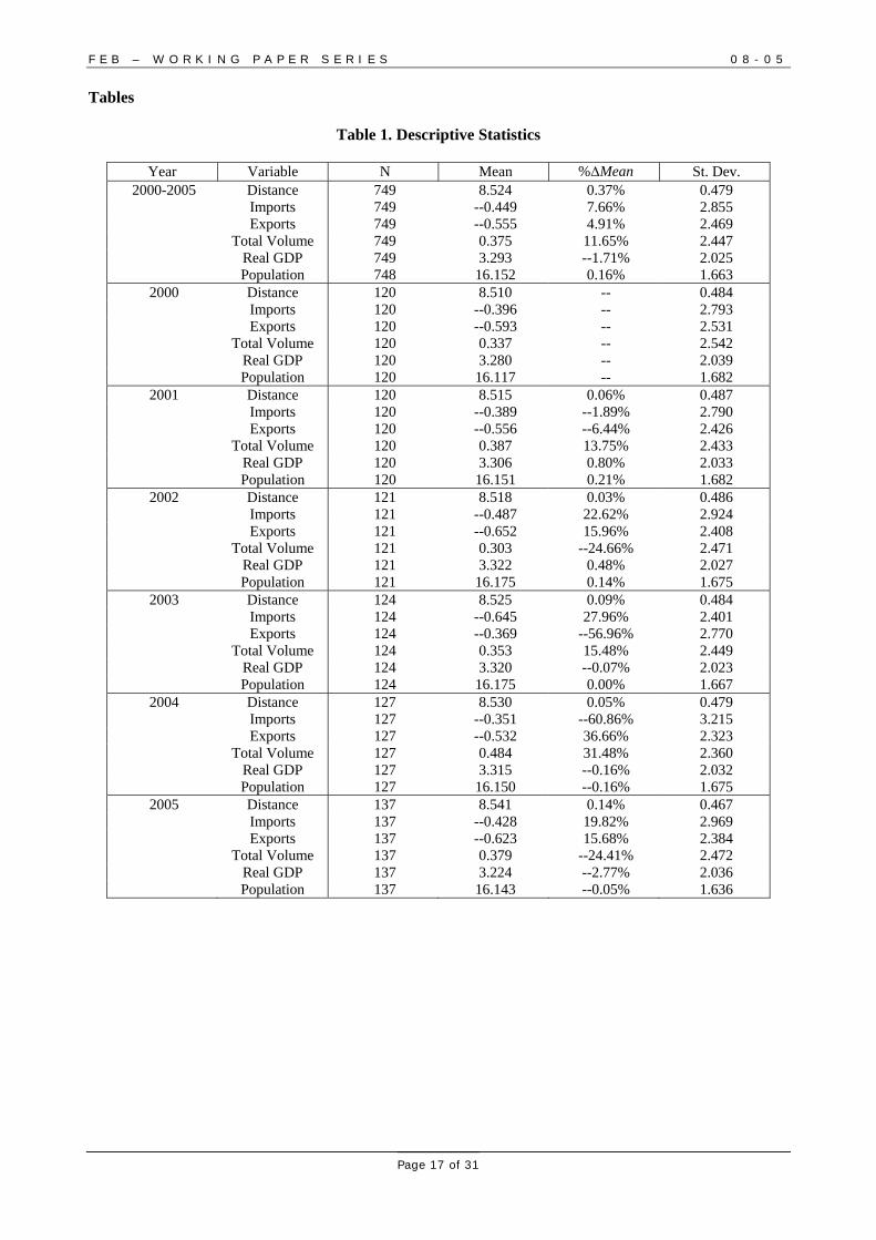
Descriptive statistics are presented in Table 1, for each year and overall for Distance, Imports,

Exports, Total Volume, Real GDP, and Population -- all of these are natural logs. The percent change

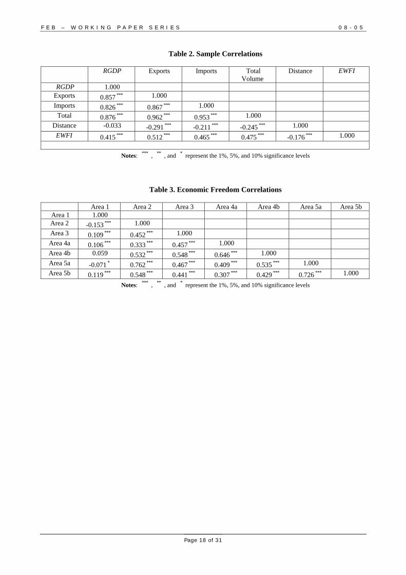
calculated for the entire period is the average of the growth over the sample period. Table 2 contains simple

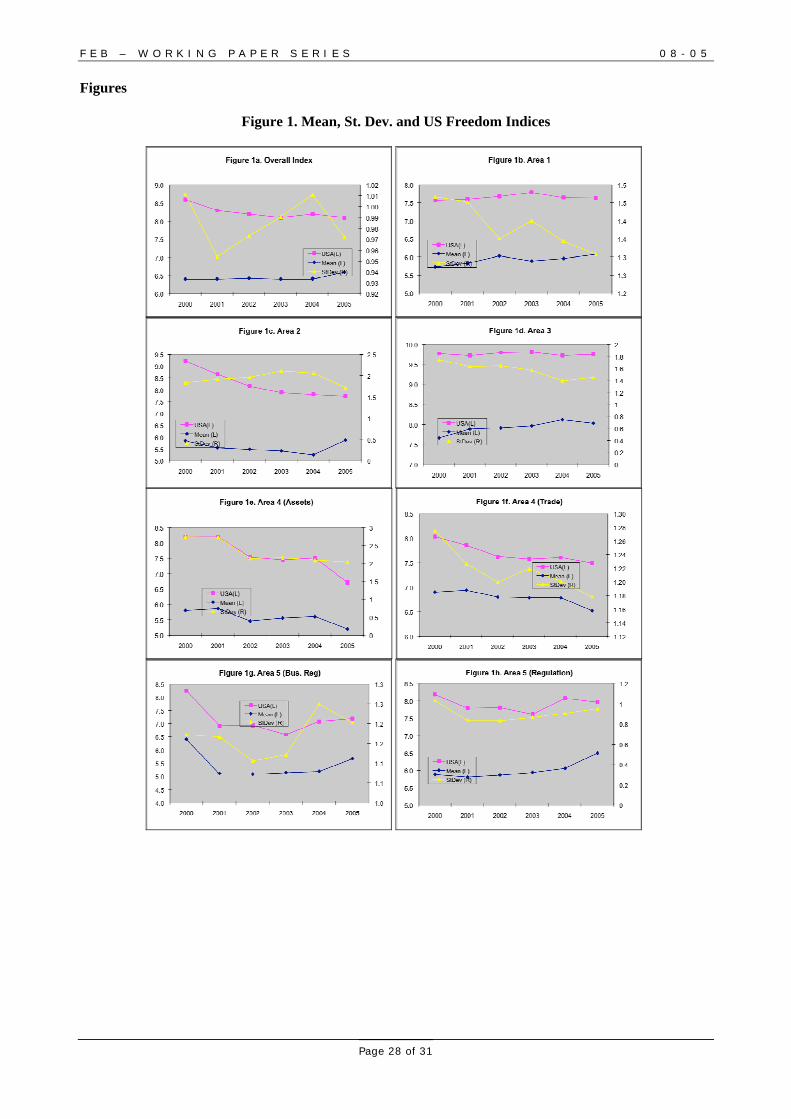
sample correlations over the entire period for the trade variables, freedom, distance and real GDP. Figure 1

shows the overall freedom index and each of the individual freedom Area Index means and the standard

deviations -- this data is not in logs. For comparison, the US indices are also included, the sample mean

and standard deviations do not include the US data.

Turning our attention first to the freedom indices in Figure 1 we note that the general trend for the means is

upwards (more freedom) with the exception of the international trade flows of goods and services and capital.

Both are falling, about 0.5 points for each, however it is also worth noting that there is less freedom in capital

movements than in trade, which is intuitively attractive given the ongoing trade negotiations reducing trade

barriers. However, it also worth noting the overall decline in the freedom of movements of both goods and assets.

We can also see no real trend in the convergence of freedom, the standard deviation of some of the

component indices is falling monetary and fiscal policy, whereas regulation seems to be diverging. The

overall index displays no discernable trend.

Looking at Table 1, we see that there are some overall trends, US trade with the rest of the world

(ROW), has, on average, been rising, despite the short down turn after 9-11-2001. On the other hand,

average real GDP has fallen, though this may have to do with the inclusion of new countries, which tend to 6 Also see de Haan and Sturm (2000), and Heckelman (2002).


Page 10 of 31

be lower income, e.g. Vietnam and Bosnia-Herzegovina. Also, continued liberalization of trade restrictions

and the realization of has led to increasing levels of trade Distance changes are due to the inclusion of new

countries, a changing composition of countries, and tectonic plate activity.

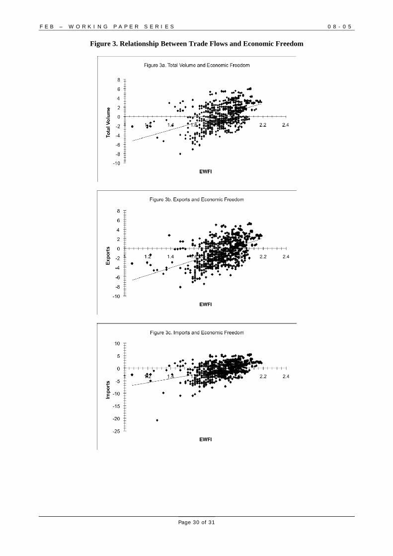
From Table 2 we can see that, we do see positive relationships between output, freedom, and the

three trade variables. Also, as expected, distance is negatively correlated to all the variables. Figures 2a-c

plot the log of the three trade variables to the log of freedom for the whole period, the line is the estimated

bivariate relationship. As can be easily seen, the scatter plots show a clear upward relationship between

each of these indices and exports and imports. Moreover, exports and imports respond differently to

economic freedom. Specifically, the scatter plot for U.S. exports is more widely distributed compared to the

plot for U.S. imports. Table 3 shows the sample correlations for the seven freedom indices. As can be seen,

correlations are rarely above 0.7, and a couple are negative.

4. Empirical Results

I begin with a gravity model which includes all the freedom indices, but not the overall index, i.e.

,''= 543210 εββββββ ++++++ lkiiii efwiefwipopydistv (4)

where all the variables are defined as before and

)5,5,4,43,2,1,(= ′bAreaaAreaaAreaaAreaAreaAreaAreaefwi

is the freedom vector. This allows us to analyze the conditional impacts of each of the areas. The vector

lkefwi captures each of the 21 interaction terms of Areas k ≠ l , k = 1,K ,5a; l = 2,K ,5b .

Results of the pooled OLS model above are presented in Table 4, time dummies have not been

tabulated. Estimated coefficients and their White adjusted −p values are presented. First we note the

standard gravity variables, real GDP and distance, are close to the literature standard, and are statistically

significant. The OECD dummy is significant and negative, evidence, perhaps, of trade diversion over the

period, while the NAFTA dummy is positive but insignificant.

Turning our attention to the freedom variables we see Areas 2, 4a, and to a lesser extent, 5a are the

relevant variables. However, Area 2, legal system and property rights is strongly negative. Area 4a, the

freedom to trade, is significantly positive. With respect to the interaction terms, we see most are not

significant, with the exception of those Area 4a, 4b, freedom of asset movements, and 5b, regulation.

Moreover, we see

0.<440,<53 22 bAaAvbAAv ∂∂∂∂∂∂

and each are statistically significant at the 1% level, or close to it.


Page 11 of 31

4.1. Results of the Pooled OLS regressions

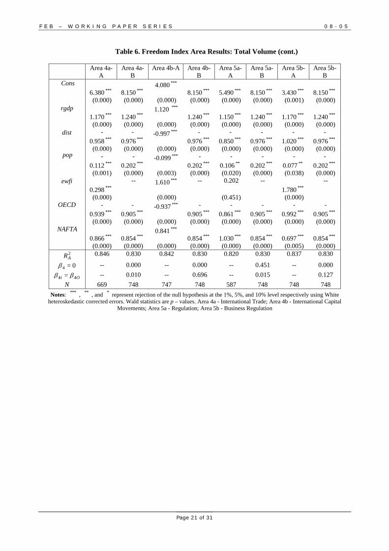
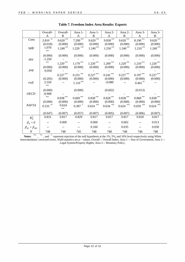
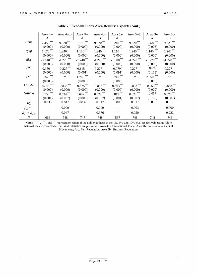
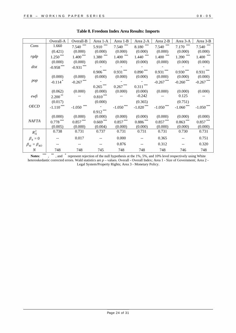
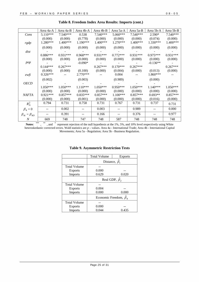
Next we consider the different Areas in isolation. Results of the pooled regressions with time

dummies can be found in Tables 5 -- 7, though the time dummy results are not tabulated for to keep clutter

to reduce clutter.7 Each Model reports two specifications: the first is an unrestricted model, `Model A', the

second restricts the parameter on economic freedom to zero, `Model B'. −p values for the −F tests of

0=4β and whether or not each freedom component can be treated as the overall index, Oi 44 = ββ , are also

presented. Heteroskedastic consistent −p values are reported in parentheses. Adjusted 2R for each

regression specification is also reported.

First, we note that, like in most gravity models, the model displays a good fit. Also, most of the

estimates are significant at the 5% level or better. This is contrast with the results in Depken and Sonora

(2005) who find that while the gravity model does a good job of estimating total volume and export trade

flows, it is less successful with imports.

A cursory glance at the results reveals that the estimated coefficients for the “standard” regressors,

real GDP and distance, all fall comfortably within the range found in the literature. Before specifically

discussing the freedom estimates, it is interesting to note that the OECD dummy yields a statistically

significant negative estimate 0.8)1.5,( −−∈ across the board with the largest effect on imports from OECD

countries. This is consistent with the US shifting its final consumer goods trade away away from similar

countries, though the time frame might be too short to capture the trade dynamics over the product cycles.

On the other hand, the NAFTA dummy is positive. In this case, the coefficient for NAFTA imports

is generally greater than for exports. Most likely this is due to the presence of Mexican tariffs on US

imports, which are scheduled to be phased out on virtually all agricultural imports by the end of 2008.

Next, we turn our attention to the estimates of the various economic freedom indicators. At first

glance, it is easy to see that there is considerable variation in the size of the elasticities of the trade values to

economic freedom. With one exception, all the estimates are positively correlated as predicted, and highly

significant. We see the overall index elasticities of freedom, 4β , to be between 1.6 and 2.5, the largest of

any of the coefficient estimates.

Interestingly, the only indicator of freedom which is negative, though not necessarily statistically

significant, is the indicator for `Legal Systems and Property Rights', Area 2, which has the implication that

countries with strong interest groups may be able to manipulate the system to their benefit, e.g. French

farmers. Perhaps, unsurprisingly, `Sound Money', Area 3, does not have much of an large impact on total

volume or imports, but does with exports, presumably because countries with relatively high degrees of

monetary autonomy closely correspond to countries which have more liberal trade, see Table 3.

7 Results are available from the author on request.


Page 12 of 31

Not surprisingly `Freedom to Trade', Area 4a, has a larger impact on trade flows than `Freedom of

Capital Movements', Area 4b, by roughly a factor of four, and both are statistically significant.

Next, consider the test statistics for 0=ˆ4β and Oi 44

ˆ=ˆ ββ . The results show that the indicator

which is most closely correlated to the overall index is `Freedom to Trade'. The data always rejects 0=ˆ4β

but never rejects the Oi 44ˆ=ˆ ββ restriction. And closer inspection of the results shows that estimates are

similar, again intuitively appealing as the biggest impact on trade flows should be overall trade policy.

Table 8 presents the the −p values for restricting the estimated coefficients for Real GDP,

Distance, and the Overall Economic Freedom Index equal to each other from each of the three dependent

variables: In the top third considers symmetric responses for Distance, jiji ≠,= 11 ββ , Real GDP,

jiji ≠,= 22 ββ , and the Freedom Index, jiji ≠,= 44 ββ , =, ji total volume, exports, imports. As can be

see, with the exception of restricting the distance estimate on imports and total volume, the data does

demonstrate considerable differences in the treatment of the exogenous variables vis-á-vis distance, real

GDP, and the Freedom Index, we can infer asymmetries do exist, particularly if we think of the total

volume as a restricted version of the overall model.

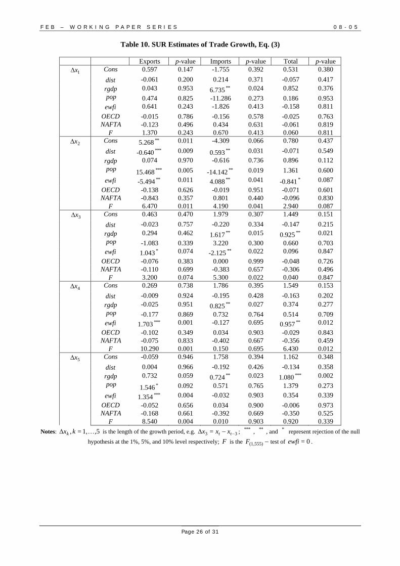
4.2. Results of the “Dynamic” Regression

Estimates from the dynamic version, using a SUR model, of the gravity model are given in Table 9.

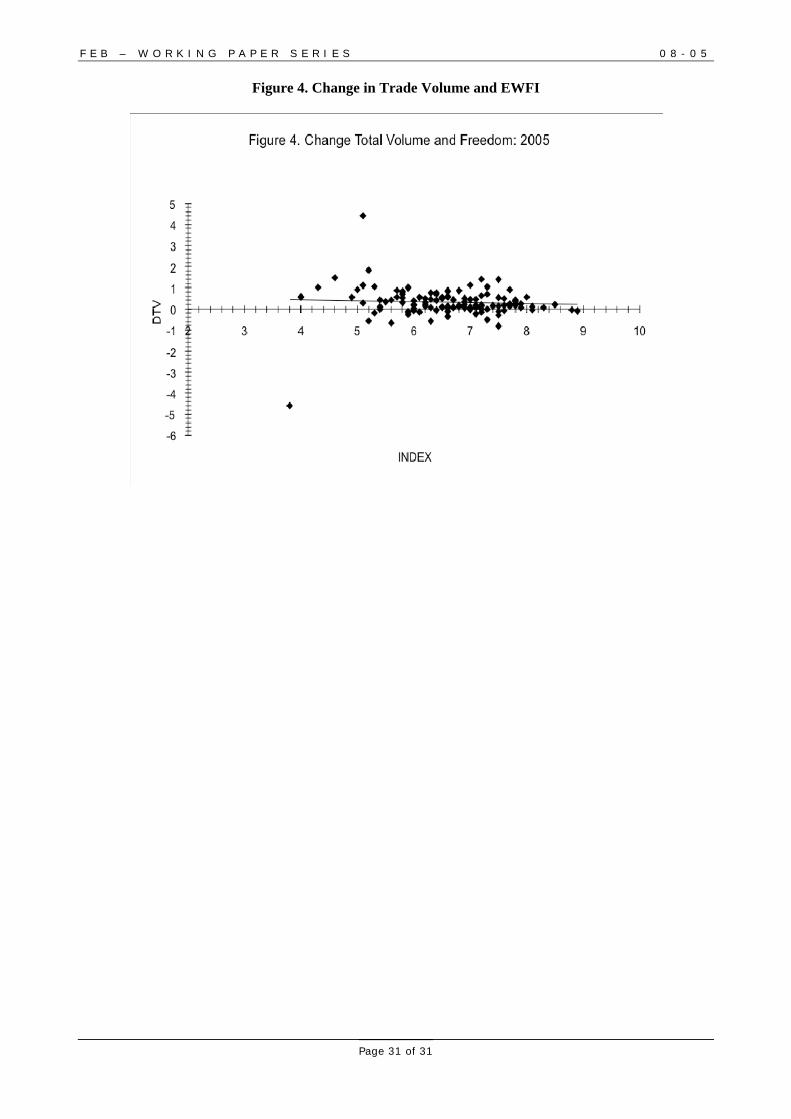
A simple two variable scatter plot of the five year growth of trade to the five year change in the EWFI,

Figure 4, shows a slight, negative relationship. For these tests I only consider the overall index. For each of

the five changes in the variables, in the first column the notation itti xxx −−∆ = is used, thus 11 = −−∆ tt xxx .

Note that the regressors are not differenced form, with the exception of distance. Estimated coefficients,

their −p values, and an F test of 0=ewfi∆ is given.

What is most notable, is which independent variables become significant over each time frame.

Thus, we notice that over shorter growth periods, one to two years, distance and population seem to play a

relatively large role, with three years of growth, economic freedom becomes statistically significant

suggesting that population growth or business cycle fluctuations, influence short term trading patterns, but

institutional/real changes to the economic structure, freedom, have longer impacts.

Additionally, freedom falls out of favor over the longer periods with respect to imports. Indeed,

longer term changes in freedom have a negative impact on imports in for 3x∆ and on, though not

significant. Also, freedom negatively impacts exports and the total volume over two year growth periods.


Page 13 of 31

What is also striking is the impact countries get from improving their freedom over the longer

periods. Generally speaking, the elasticities of freedom are substantially greater than those for real GDP

growth and, with the exception of two year growth, population.

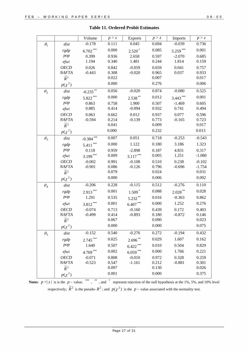
4.3. Ordered Probit Regression

To investigate the effects of changes in output, population and economic freedom on the

probability that trade flows will increase. Under the assumption that errors are standard normal consider the

following model:

,51,=;'= ,, Kkzefi kttktktt εγβαθ +∆+∆+ −−− (5)

where ktt −,θ is an indicator variable with the properties

⎪⎩

⎪⎨

⎧

∆∆∆∈∆

≤∆

−−

−−

−

−

,>2](0,1

0,0=

,,

,,

,

,

kttktt

kttktt

ktt

ktt

vvifvvif

vifθ

β̂ , the estimated coefficient of most interest, and, ex ante, should be positive, a higher index increases the

probability of further trade; kttv −∆ , is the average growth of the trade variables, and is expected to be larger

as we extend the time of the lag; ),,,,(= ′NAFTAOECDdistpoprgdpz is a vector of country characteristics as

define in equation ((2)), γ is a vector of characteristic coefficients and ε ~ (0,1). As before, changes in any

of the explanatory variables may take time to “bleed” into invigorated trade, so we define the growth in any

variable x to be defined over ,51,= Kk lags: kttt xxx −−∆ = .

Results of the ordered probit model can be found in Table 11. Unfortunately, the estimated

coefficients from probit are difficult to interpret, though they have a similar explanation or a binary OLS

model's estimated coefficients, which are understood as a probabilities. Essentially, the probit model

defines the dependent variable θ as given by

))()1((ln= TradePTradeP −θ

where )(TradeP is the probability of increased trade. Thus we can only concentrate on estimated signs and

the size of the coefficients.

What is striking is how the significance of the independent variables change as we extend the

length of time. Over the short term, two years or less, real GDP is the only variable which is statistically

significant. However, once we lengthen years the lag of growth, the freedom coefficients become more

important, particularly for exports. We also note that the magnitudue of the freedom coefficients relative to

the other variables as we increase the lag, implying a greater probability for increase trade flows as the

result of more freedom. This result has the intuitively attractive result that in the shorter term, trade increase


Page 14 of 31

simply due to increases in incomes, but over the longer term improvements in welfare are due to changes in

the economic structure of an economy.

The results suggest that economies which experience rapid short term growth will have a larger

probability of increased trade volume. But, if this growth is not accompanied by longer term changes in

freedom, any increases achieved by economic growth cannot sustain increased trade flows. Put another

way, to ensure the probability of robust medium term trade growth a country must implement institutional

changes which impact freedom.

For countries which have experienced rapid GDP growth and commensurate trade growth without

implementing other reforms, such as China which EFI is below the mean, the analysis indicates that to

enjoy longer term expansion, changes in policy to ensure greater freedom be put in place.

Given the length of the data, we cannot make inference the time frame required to fully enjoy the

fruits of the policy changes, but the current analysis suggests that even the relatively short time span of six

years, there is evidence of the effects of institutional changes on trade.

5. Summary

This paper examines the impacts of economic freedom within the context of a standard gravity

model. Using a single country model, the gravity model can also investigate the asymmetries of trade

between the United States and her trading partners. It is clear from the estimates that if the gains to the

United States are any indication, and given that the US accounts for about about 12% of merchandise and

13% of services trade, we can imagine what the scope of welfare improvement would be should we conduct

similar studies on world trade.

The results also suggest that even if countries concentrate on one of the areas of freedom they can

enjoy an increase in their overall welfare through the expansion of trade. However, it does depend on which

of the freedom indicators a country chooses to concentrate one.

While economic improvement of the masses may come at the detriment of those who hold political

power and those who benefit from the rents generated by less economic freedom, the methods by which

economic improvement improves are left to those with a comparative advantage in that area.

References

1. Anderson, James E. (1979). “A Theoretical Foundation for the Gravity Equation,” American

Economic Review, 69, 106-116.

2. Anderson, James E. (1985). “The Relative Inefficiency of Quotas: The Cheese Case,” American

Economic Review, 75, 178-90.


Page 15 of 31

3. Anderson, James E. and Douglas Marcouiller (2002). “Insecurity and the Pattern of Trade: An

Empirical Investigation,” Review of Economics and Statistics, 84, 342-352.

4. Anderson, James E. and Eric van Wincoop (2004). “Trade Costs,” Journal of Economic Literature,

42, 691-751.

5. Barro, Robert (1991). “Economic Growth in a Cross-Section of Countries,” Quarterly Journal of

Economics, 106(2), 407-43.

6. Bauer, Peter (2000). From Subsistence to Exchange and Other Essays, Princeton: Princeton

University Press.

7. Bergstrand, Jeffrey H. (1985). “The Gravity Equation in International Trade: Some Microeconomic

Foundations and Empirical Evidence,” Review of Economics and Statistics, 67, 474-81.

8. Blomberg, S. Brock and Gregory D. Hess (2006). “How Does Violence Tax Trade?” Review of

Economics and Statistics, 88, 599-612.

9. Clark, J.R. and Dwight R. Lee (2006). “Freedom, Entrepreneurship and Economic Progress,”

Journal of Entrepreneurship, 15, 1-17.

10. De Haan, J. and J-E. Sturm (2000). “On the Relationship Between Economic Freedom and Economic

Growth,” European Journal of Political Economy, 16, 215-241.

11. Depken, C A., C. LaFountain and R. Butters (2007). “Corruption and Creditworthiness: Evidence

from Sovereign Credit Ratings,” mimeo, Department of Economics University of Texas - Arlington.

12. Depken, C.A. and L. C. Simmons (2004). “Social construct and the propensity for software piracy,”

Applied Economics Letters, 11, 97-100.

13. Depken, C.A. and R.J. Sonora (2005). “Asymmetric Effects of Economic Freedom on International

Trade Flows,” International Journal of Business and Economics, 4, 141-155.

14. Easton, Steven T., and Michael A. Walker (1997). “Income, Growth, and Economic Freedom,”

American Economic Review, 87, 328-32.

15. Engel, Charles and John H. Rogers (1996), “How Wide is the Border?,” The American Economic

Review, 86, 1112-1125.

16. Evenett, Simon J and Wolfgang Keller (1998). “On Theories Explaining the Success of the Gravity

Equation,” National Bureau of Economic Research, Working Paper 6529.

17. Farr, W. Ken, Richard A. Lord, and J. Larry Wolfenbarger (1998). “Economic Freedom, Political

Freedom and Economic Well-Being,” Cato Journal, 18, 247-262.

18. Feenstra, Robert C., James R. Markusen, and Andrew K. Rose (2001). Using the Gravity Equation to

differentiate Between Alternative Theories of Trade,” Canadian Journal of Economics. 34, 430-447.

19. Fergusson, Leopold (2006). “Institutions for Financial Development: What Are They and Where Do

They Come From?” Journal of Economic Surveys, 20, 27 -- 69.

20. Greenaway, David, Wyn Morgan, and Peter Wright, (2001). “Trade Liberalisation and Growth in

Developing Countries,” Journal of Development Economics, 67, 229-244.


Page 16 of 31

21. Gwartney, James Robert Lawson (2007). Economic Freedom of the World: 2007 Annual Report,

Vancouver: The Fraser Institute. Data retrieved from www.freetheworld.com

22. Hanke, Steve H., and Stephen J.K. Walters (1997). “Economic Freedom, Prosperity, and Equality: A

Survey,” Cato Journal, 17, 117-146.

23. Heckelman, Jac C. (2002). “On the Measurement of Comparative Economic Freedom across

Nations,” International Journal of Business and Economics, 1, 251-261.

24. Hayek, Friedrich (1937). “Economics and Knowledge,” Economica, 4, 33-54.

25. Hayek, Friedrich (1989). “The Pretence of Knowledge,” The American Economic Review, 79, 3-7.

26. Krugman, Paul R. and Maurice Obstfeld (2003). International Economics: Theory and Policy, 6th

Edition, Addison Wesley, 2003.

27. Leeson, Peter T. and Russell S. Sobel (2006). “Contagious Capitalism”, mimeo, Department of

Economics, West Virginia University.

28. Office of Trade and Economic Analysis, U.S. Department of Commerce (OTEA) (2002).

http://www.ita.doc.gov/td/industry/otea/

29. Ovaska, Tomi and Russell Sobel (2005). “Entrepeneurship in Post-Socialist Countries,” Journal of

Private Enterprise, 21, 8-28.

30. Martínez-Zarzoso, I. F. Nowak-Lehmann D. and N. Horsewood (2006). “Effects of Regional Trade

Agreements Using a Static and Dynamic Gravity Equation,” Working paper, No.149, Ibero-America

Institute for Economic Research, Georg-August-Universität Göttingen.

31. Pöyhönen, Pentti (1963). “A Tentative Model for the Volume of Trade Between Countries,”

Weltwirtshaftliches Archive, 90, 93-100.

32. Quarterly Journal of Economics (1993), CVIII, Special Issue on growth.

33. Soloaga, Isidro and L. Alan Winters (2001). “Regionalism in the nineties: What effect on trade?,”

North American Journal of Economics and Finance, 12, 1–29.

34. Summary, Rebecca M. (1989). “A Political-Economic Model of U.S. Bilateral Trade,” The Review of

Economics and Statistics, 71, 179-182.

35. Tinbergen, J. (1962). The World Economy. Suggestions for an International Economic Policy, New

York, NY: Twentieth Century Fund.

36. Wall, Howard J. (1999). “Using the Gravity Model to Estimate the Costs of Protection,” Review,

January/February, Federal Reserve Bank of St. Louis, 33-40.

37. Wall, Howard J. (2000). “Gravity Model Specification and the Effects of the Canada-U.S. Border,”

Federal Reserve Bank of St. Louis working paper, 2000-2024A.

38. Wolf, Holger C. (2000). “Intranational Home Bias in Trade,” Review of Economics and Statistics,

LXXXII, November, 555-563.


Page 17 of 31

Tables

Table 1. Descriptive Statistics

Year Variable N Mean Mean∆% St. Dev. 2000-2005 Distance 749 8.524 0.37% 0.479

Imports 749 --0.449 7.66% 2.855 Exports 749 --0.555 4.91% 2.469 Total Volume 749 0.375 11.65% 2.447 Real GDP 749 3.293 --1.71% 2.025 Population 748 16.152 0.16% 1.663

2000 Distance 120 8.510 -- 0.484 Imports 120 --0.396 -- 2.793 Exports 120 --0.593 -- 2.531 Total Volume 120 0.337 -- 2.542 Real GDP 120 3.280 -- 2.039 Population 120 16.117 -- 1.682

2001 Distance 120 8.515 0.06% 0.487 Imports 120 --0.389 --1.89% 2.790 Exports 120 --0.556 --6.44% 2.426 Total Volume 120 0.387 13.75% 2.433 Real GDP 120 3.306 0.80% 2.033 Population 120 16.151 0.21% 1.682

2002 Distance 121 8.518 0.03% 0.486 Imports 121 --0.487 22.62% 2.924 Exports 121 --0.652 15.96% 2.408 Total Volume 121 0.303 --24.66% 2.471 Real GDP 121 3.322 0.48% 2.027 Population 121 16.175 0.14% 1.675

2003 Distance 124 8.525 0.09% 0.484 Imports 124 --0.645 27.96% 2.401 Exports 124 --0.369 --56.96% 2.770 Total Volume 124 0.353 15.48% 2.449 Real GDP 124 3.320 --0.07% 2.023 Population 124 16.175 0.00% 1.667

2004 Distance 127 8.530 0.05% 0.479 Imports 127 --0.351 --60.86% 3.215 Exports 127 --0.532 36.66% 2.323 Total Volume 127 0.484 31.48% 2.360 Real GDP 127 3.315 --0.16% 2.032 Population 127 16.150 --0.16% 1.675

2005 Distance 137 8.541 0.14% 0.467 Imports 137 --0.428 19.82% 2.969 Exports 137 --0.623 15.68% 2.384 Total Volume 137 0.379 --24.41% 2.472 Real GDP 137 3.224 --2.77% 2.036 Population 137 16.143 --0.05% 1.636


Page 18 of 31

Table 2. Sample Correlations

RGDP Exports Imports Total

Volume Distance EWFI

RGDP 1.000 Exports 0.857 *** 1.000 Imports 0.826 *** 0.867 *** 1.000

Total 0.876 *** 0.962 *** 0.953 *** 1.000 Distance -0.033 -0.291 *** -0.211 *** -0.245 *** 1.000

EWFI 0.415 *** 0.512 *** 0.465 *** 0.475 *** -0.176 *** 1.000

Notes: *** , ** , and * represent the 1%, 5%, and 10% significance levels

Table 3. Economic Freedom Correlations

Area 1 Area 2 Area 3 Area 4a Area 4b Area 5a Area 5b Area 1 1.000 Area 2 -0.153 *** 1.000 Area 3 0.109 *** 0.452 *** 1.000 Area 4a 0.106 *** 0.333 *** 0.457 *** 1.000 Area 4b 0.059 0.532 *** 0.548 *** 0.646 *** 1.000 Area 5a -0.071 * 0.762 *** 0.467 *** 0.409 *** 0.535 *** 1.000 Area 5b 0.119 *** 0.548 *** 0.441 *** 0.307 *** 0.429 *** 0.726 *** 1.000

Notes: *** , ** , and * represent the 1%, 5%, and 10% significance levels


Page 19 of 31

Table 4. Unrestricted Pooled OLS Results

TV −P value Exports −P value Imports −P value Cons -9.152 0.241 -3.229 0.680 -9.772 0.361 rgdp 1.042 *** 0.000 1.022 *** 0.000 1.149 *** 0.000 dist -0.968 *** 0.000 -1.159 *** 0.000 -0.896 *** 0.000 pop -0.013 0.816 0.032 0.575 -0.069 0.329

1Area -3.269 0.358 -4.011 0.297 -2.063 0.651 2Area -12.735 *** 0.000 -10.606 *** 0.000 -10.648 *** 0.006 3Area 3.745 0.196 3.913 0.164 -0.643 0.863 aArea4 7.108 *** 0.001 5.750 ** 0.014 10.241 *** 0.002 bArea4 -0.928 0.828 -5.925 0.173 -0.944 0.871 aArea5 8.026 * 0.058 6.734 0.161 11.586 ** 0.047 bArea5 10.187 0.112 9.380 0.178 5.538 0.536

OECD -0.734 *** 0.000 -0.726 *** 0.000 -0.857 *** 0.000 NAFTA 0.301 0.138 0.161 0.522 0.384 0.136 12A 0.342 0.647 0.134 0.881 0.274 0.751

13A 0.856 0.290 -0.254 0.763 1.128 0.263 aA14 -1.829 *** 0.001 -1.109 * 0.077 -1.947 *** 0.004 bA14 1.832 0.319 3.192 0.124 1.929 0.411 aA15 -1.362 0.200 0.210 0.853 -1.655 0.233 bA15 2.173 0.252 0.437 0.841 1.431 0.515

23A 1.453 0.180 -0.215 0.856 1.795 0.206 aA24 0.032 0.923 -0.265 0.553 0.110 0.799 bA24 1.174 0.254 2.496 * 0.055 1.430 0.299 aA25 0.964 0.109 1.187 0.058 1.281 0.127 bA25 2.688 ** 0.029 2.392 * 0.079 0.479 0.796 aA34 -0.895 0.273 -0.086 0.915 -1.866 * 0.080 bA34 3.777 *** 0.002 3.568 *** 0.005 5.108 *** 0.002 aA35 0.155 0.909 -0.232 0.868 -0.264 0.884 bA35 -7.988 *** 0.000 -5.392 *** 0.007 -6.398 ** 0.012 baA 44 -3.354 *** 0.000 -2.546 ** 0.016 -4.701 *** 0.001 aaA 54 0.494 0.441 0.365 0.628 0.563 0.526 baA 54 1.756 0.119 0.484 0.693 2.519 * 0.097 abA 54 -1.740 0.399 -2.562 0.277 -4.263 0.136 bbA 54 0.017 0.995 0.198 0.955 1.992 0.647 baA 55 -2.709 0.151 -2.184 0.288 -1.619 0.512

2R 0.879 0.861 0.827

Notes: Time dummies suppressed; *** , ** , and * represent rejection of the null hypothesis at the 1%, 5%, and 10% level respectively using White heteroskedastic corrected errors. ,,,52,=,51,=, lKlKl ≠mbamAm where m and l index the

different freedom indices are the interaction variables.


Page 20 of 31

Table 5. Freedom Index Area Results: Total Volume

Overall-A Overall-B Area 1-A Area 1-B Area 2-A Area 2-B Area 3-A Area 3-B Cons 3.780 *** 8.150 *** 6.280 *** 8.150 *** 9.010 *** 8.150 *** 8.130 *** 8.150 ***

(0.001) (0.000) (0.000) (0.000) (0.000) (0.000) (0.000) (0.000) rgdp 1.140 *** 1.240 *** 1.230 *** 1.240 *** 1.300 *** 1.240 *** 1.240 *** 1.240 ***

(0.000) (0.000) (0.000) (0.000) (0.000) (0.000) (0.000) (0.000) dist -0.997 *** -0.976 *** -0.940 *** -0.976 *** 0.922 *** -0.976 *** -0.974 *** -0.976 ***

(0.000) (0.000) (0.000) (0.000) (0.000) (0.000) (0.000) (0.000) pop -0.089 ** -0.202 *** -0.204 *** -0.202 *** -0.261 *** -0.202 *** -0.200 *** -0.202 ***

(0.025) (0.000) (0.000) (0.000) (0.000) (0.000) (0.000) (0.000) ewfi 1.630 *** -- 0.900 *** -- --0.325 ** -- 0.000 --

(0.000) (0.000) (0.036) (0.998) OECD --0.950 *** -0.905 *** -0.763 *** -0.905 *** -0.865 *** -0.905 *** -0.905 *** -0.905 ***

(0.000) (0.000) (0.000) (0.000) (0.000) (0.000) (0.000) (0.000) NAFTA 0.795 *** 0.854 *** 0.654 *** 0.854 *** 0.892 *** 0.854 *** 0.857 *** 0.854 ***

(0.000) (0.000) (0.000) (0.000) (0.000) (0.000) (0.000) (0.000) 2

AR 0.835 0.830 0.839 0.830 0.831 0.830 0.829 0.830

0=4β -- 0.000 -- 0.000 -- 0.036 -- 0.998

Oi 44 = ββ

-- -- -- 0.057 -- 0.006 -- 0.006

N 748 748 745 748 748 748 746 748 Notes: *** , ** , and * represent rejection of the null hypothesis at the 1%, 5%, and 10% level respectively using White

heteroskedastic corrected errors. Wald statistics are p – values. Overall - Overall Index; Area 1 - Size of Government; Area 2 - Legal System/Property Rights; Area 3 - Monetary Policy.


Page 21 of 31

Table 6. Freedom Index Area Results: Total Volume (cont.)

Area 4a-

A Area 4a-

B Area 4b-A Area 4b-

B Area 5a-

A Area 5a-

B Area 5b-

A Area 5b-

B Cons

6.380 ***

8.150 *** 4.080 ***

8.150 ***

5.490 ***

8.150 ***

3.430 ***

8.150 *** (0.000) (0.000) (0.000) (0.000) (0.000) (0.000) (0.001) (0.000)

rgdp 1.170 ***

1.240 ***

1.120 *** 1.240 ***

1.150 ***

1.240 ***

1.170 ***

1.240 ***

(0.000) (0.000) (0.000) (0.000) (0.000) (0.000) (0.000) (0.000) dist -

0.958 *** -

0.976 *** -0.997 *** -

0.976 *** -

0.850 *** -

0.976 *** -

1.020 *** -

0.976 *** (0.000) (0.000) (0.000) (0.000) (0.000) (0.000) (0.000) (0.000)

pop -0.112 ***

-0.202 ***

-0.099 *** -0.202 ***

-0.106 **

-0.202 ***

-0.077 **

-0.202 ***

(0.001) (0.000) (0.003) (0.000) (0.020) (0.000) (0.038) (0.000) ewfi

0.298 *** -- 1.610 *** -- 0.202 --

1.780 *** --

(0.000) (0.000) (0.451) (0.000) OECD -

0.939 *** -

0.905 *** -0.937 *** -

0.905 *** -

0.861 *** -

0.905 *** -

0.992 *** -

0.905 *** (0.000) (0.000) (0.000) (0.000) (0.000) (0.000) (0.000) (0.000)

NAFTA 0.866 ***

0.854 ***

0.841 *** 0.854 ***

1.030 ***

0.854 ***

0.697 ***

0.854 ***

(0.000) (0.000) (0.000) (0.000) (0.000) (0.000) (0.005) (0.000) 2AR 0.846 0.830 0.842 0.830 0.820 0.830 0.837 0.830

0=4β -- 0.000 -- 0.000 -- 0.451 -- 0.000

Oi 44 = ββ -- 0.010 -- 0.696 -- 0.015 -- 0.127 N 669 748 747 748 587 748 748 748

Notes: *** , ** , and * represent rejection of the null hypothesis at the 1%, 5%, and 10% level respectively using White heteroskedastic corrected errors. Wald statistics are p – values. Area 4a - International Trade; Area 4b - International Capital

Movements; Area 5a - Regulation; Area 5b - Business Regulation


Page 22 of 31

Table 7. Freedom Index Area Results: Exports

Overall-

A Overall-

B Area 1-

A Area 1-

B Area 2-

A Area 2-

B Area 3-

A Area 3-

B Cons 2.810 ** 9.620 *** 7.290 *** 9.620 *** 9.830 *** 9.620 *** 8.190 *** 9.620 ***

(0.018) (0.000) (0.000) (0.000) (0.000) (0.000) (0.000) (0.000) rgdp 1.070

*** 1.240 *** 1.220 *** 1.240 *** 1.250 *** 1.240 *** 1.210 *** 1.240 ***

(0.000) (0.000) (0.000) (0.000) (0.000) (0.000) (0.000) (0.000) dist -1.250

*** -

1.220 *** -

1.170 *** -

1.220 *** -

1.200 *** -

1.220 *** -

1.210 *** -

1.220 *** (0.000) (0.000) (0.000) (0.000) (0.000) (0.000) (0.000) (0.000)

pop -0.050 -0.227 ***

-0.231 ***

-0.227 ***

-0.241 ***

-0.227 ***

-0.197 ***

-0.227 ***

(0.205) (0.000) (0.000) (0.000) (0.000) (0.000) (0.000) (0.000) ewfi 2.550

*** -- 1.110 *** -- -0.080 -- 0.461 ** --

(0.000) (0.000) (0.602) (0.013) OECD -0.908

*** -

0.838 *** -

0.669 *** -

0.838 *** -

0.828 *** -

0.838 *** -

0.868 *** -

0.838 *** (0.000) (0.000) (0.000) (0.000) (0.000) (0.000) (0.000) (0.000)

NAFTA 0.533 ** 0.624 ***

0.387 * 0.624 *** 0.634 *** 0.624 *** 0.659 *** 0.624 ***

(0.047) (0.007) (0.057) (0.007) (0.005) (0.007) (0.006) (0.007) 2

AR 0.831 0.817 0.829 0.817 0.817 0.817 0.818 0.817

0=4β -- 0.000 -- 0.000 -- 0.602 -- 0.013

Oi 44 = ββ -- -- -- 0.160 -- 0.035 -- 0.030 N 748 748 745 748 748 748 746 748

Notes: *** , ** , and * represent rejection of the null hypothesis at the 1%, 5%, and 10% level respectively using White heteroskedastic corrected errors. Wald statistics are p – values. Overall -- Overall Index; Area 1 -- Size of Government; Area 2 --

Legal System/Property Rights; Area 3 -- Monetary Policy.


Page 23 of 31

Table 7. Freedom Index Area Results: Exports (cont.)

Area 4a-

A Area 4a-B Area 4b-

A Area 4b-

B Area 5a-

A Area 5a-B Area 5b-

A Area 5b-

B Cons 7.450 *** 9.620 *** 5.190 *** 9.620 *** 5.240 *** 9.620 *** 3.370 *** 9.620 ***

(0.000) (0.000) (0.000) (0.000) (0.000) (0.000) (0.003) (0.000) rgdp 1.170 *** 1.240 *** 1.100 *** 1.240 *** 1.110 *** 1.240 *** 1.140 *** 1.240 ***

(0.000) (0.000) (0.000) (0.000) (0.000) (0.000) (0.000) (0.000) dist -1.140 *** -1.220 *** -1.240 *** -1.220 *** -1.080 *** -1.220 *** -1.270 *** -1.220 ***

(0.000) (0.000) (0.000) (0.000) (0.000) (0.000) (0.000) (0.000) pop -0.150 *** -0.227 *** -0.115 *** -0.227 *** -0.079 * -0.227 *** -0.061 -0.227 ***

(0.000) (0.000) (0.001) (0.000) (0.091) (0.000) (0.113) (0.000) ewfi 0.348 *** -- 1.760 *** -- 0.747 *** -- 2.350 *** --

(0.000) (0.000) (0.003) (0.000) OECD -0.921 *** -0.838 *** -0.875 *** -0.838 *** -0.863 *** -0.838 *** -0.953 *** -0.838 ***

(0.000) (0.000) (0.000) (0.000) (0.000) (0.000) (0.000) (0.000) NAFTA 0.750 *** 0.624 *** 0.607 *** 0.624 *** 0.819 *** 0.624 *** 0.417 0.624 ***

(0.001) (0.007) (0.008) (0.007) (0.001) (0.007) (0.156) (0.007) 2AR 0.836 0.817 0.832 0.817 0.809 0.817 0.830 0.817

0=4β -- 0.000 -- 0.000 -- 0.003 -- 0.000

Oi 44 = ββ -- 0.047 -- 0.976 -- 0.050 -- 0.222 N 669 748 747 748 587 748 748 748


Movements; Area 5a - Regulation; Area 5b - Business Regulation.


Page 24 of 31

Table 8. Freedom Index Area Results: Imports

Overall-A Overall-B Area 1-A Area 1-B Area 2-A Area 2-B Area 3-A Area 3-B

Cons 1.660 7.540 *** 5.910 *** 7.540 *** 8.180 *** 7.540 *** 7.170 *** 7.540 *** (0.421) (0.000) (0.000) (0.000) (0.000) (0.000) (0.000) (0.000)

rgdp 1.250 *** 1.400 *** 1.380 *** 1.400 *** 1.440 *** 1.400 *** 1.390 *** 1.400 *** (0.000) (0.000) (0.000) (0.000) (0.000) (0.000) (0.000) (0.000)

dist -0.958 *** -0.931 *** -0.906 ***

-0.931 ***

-0.890 ***

-0.931 ***

-0.930 ***

-0.931 ***

(0.000) (0.000) (0.000) (0.000) (0.000) (0.000) (0.000) (0.000) pop -0.114 * -0.267 *** -

0.265 *** -

0.267 *** -

0.311 *** -0.267 *** -0.260 *** -0.267 ***

(0.062) (0.000) (0.000) (0.000) (0.000) (0.000) (0.000) (0.000) ewfi 2.200 ** -- 0.810 *** -- -0.242 -- 0.125 --

(0.017) (0.000) (0.365) (0.751) OECD -1.110 *** -1.050 *** -

0.912 *** -1.050 *** -1.020 *** -1.050 *** -1.060 *** -1.050 ***

(0.000) (0.000) (0.000) (0.000) (0.000) (0.000) (0.000) (0.000) NAFTA 0.778 *** 0.857 *** 0.669 *** 0.857 *** 0.886 *** 0.857 *** 0.863 *** 0.857 ***

(0.005) (0.000) (0.004) (0.000) (0.000) (0.000) (0.000) (0.000) 2AR 0.738 0.731 0.737 0.731 0.731 0.731 0.730 0.731

0=4β -- 0.017 -- 0.000 -- 0.365 -- 0.751

Oi 44 = ββ -- -- -- 0.876 -- 0.312 -- 0.320 N 748 748 745 748 748 748 746 748

Notes: *** , ** , and * represent rejection of the null hypothesis at the 1%, 5%, and 10% level respectively using White heteroskedastic corrected errors. Wald statistics are p – values. Overall - Overall Index; Area 1 - Size of Government; Area 2 -

Legal System/Property Rights; Area 3 - Monetary Policy.


Page 25 of 31

Table 8. Freedom Index Area Results: Imports (cont.)

Area 4a-A Area 4a-B Area 4b-A Area 4b-B Area 5a-A Area 5a-B Area 5b-A Area 5b-B Cons 5.110*** 7.540*** 0.538 7.540*** 5.060*** 7.540*** 2.590* 7.540***

(0.000) (0.000) (0.778) (0.000) (0.000) (0.000) (0.074) (0.000) rgdp 1.280*** 1.400*** 1.190*** 1.400*** 1.270*** 1.400*** 1.330*** 1.400***

(0.000) (0.000) (0.000) (0.000) (0.000) (0.000) (0.000) (0.000) dist -

0.886*** -

0.931*** -

0.968*** -

0.931*** -

0.772*** -

0.931*** -

0.975*** -

0.931*** (0.000) (0.000) (0.000) (0.000) (0.000) (0.000) (0.000) (0.000)

pop -0.144***

-0.267***

-0.090* -0.267***

-0.170***

-0.267***

-0.136** -0.267***

(0.000) (0.000) (0.100) (0.000) (0.004) (0.000) (0.013) (0.000) ewfi 0.326*** -- 2.770*** -- 0.004 -- 1.860*** --

(0.002) (0.003) (0.989) (0.000) OECD -

1.050*** -

1.050*** -

1.110*** -

1.050*** -

0.950*** -

1.050*** -

1.140*** -

1.050*** (0.000) (0.000) (0.000) (0.000) (0.000) (0.000) (0.000) (0.000)

NAFTA 0.921*** 0.857*** 0.835*** 0.857*** 1.100*** 0.857*** 0.693** 0.857*** (0.000) (0.000) (0.001) (0.000) (0.000) (0.000) (0.016) (0.000)

2AR 0.794 0.731 0.758 0.731 0.767 0.731 0.737 0.731

0=4β -- 0.002 -- 0.003 -- 0.989 -- 0.000

Oi 44 = ββ -- 0.391 -- 0.166 -- 0.376 -- 0.977 N 669 748 747 748 587 748 748 748


Movements; Area 5a - Regulation; Area 5b - Business Regulation.

Table 9. Asymmetric Restriction Tests

Total Volume Exports Distance, 1β̂

Total Volume -- Exports 0.000 -- Imports 0.629 0.020

Real GDP, 2β̂ Total Volume --

Exports 0.004 -- Imports 0.000 0.000

Economic Freedom, 4β̂ Total Volume --

Exports 0.000 -- Imports 0.044 0.435


Page 26 of 31

Table 10. SUR Estimates of Trade Growth, Eq. (3)

Exports p-value Imports p-value Total p-value 1x∆ Cons 0.597 0.147 -1.755 0.392 0.531 0.380

dist -0.061 0.200 0.214 0.371 -0.057 0.417 rgdp 0.043 0.953 6.735 ** 0.024 0.852 0.376 pop 0.474 0.825 -11.286 0.273 0.186 0.953 ewfi 0.641 0.243 -1.826 0.413 -0.158 0.811 OECD -0.015 0.786 -0.156 0.578 -0.025 0.763 NAFTA -0.123 0.496 0.434 0.631 -0.061 0.819 F 1.370 0.243 0.670 0.413 0.060 0.811

2x∆ Cons 5.268 ** 0.011 -4.309 0.066 0.780 0.437 dist -0.640 *** 0.009 0.593 ** 0.031 -0.071 0.549 rgdp 0.074 0.970 -0.616 0.736 0.896 0.112 pop 15.468 *** 0.005 -14.142 ** 0.019 1.361 0.600 ewfi -5.494 ** 0.011 4.088 ** 0.041 -0.841 * 0.087 OECD -0.138 0.626 -0.019 0.951 -0.071 0.601 NAFTA -0.843 0.357 0.801 0.440 -0.096 0.830 F 6.470 0.011 4.190 0.041 2.940 0.087

3x∆ Cons 0.463 0.470 1.979 0.307 1.449 0.151 dist -0.023 0.757 -0.220 0.334 -0.147 0.215 rgdp 0.294 0.462 1.617 ** 0.015 0.925 ** 0.021 pop -1.083 0.339 3.220 0.300 0.660 0.703 ewfi 1.043 * 0.074 -2.125 ** 0.022 0.096 0.847 OECD -0.076 0.383 0.000 0.999 -0.048 0.726 NAFTA -0.110 0.699 -0.383 0.657 -0.306 0.496 F 3.200 0.074 5.300 0.022 0.040 0.847

4x∆ Cons 0.269 0.738 1.786 0.395 1.549 0.153 dist -0.009 0.924 -0.195 0.428 -0.163 0.202 rgdp -0.025 0.951 0.825 ** 0.027 0.374 0.277 pop -0.177 0.869 0.732 0.764 0.514 0.709 ewfi 1.703 *** 0.001 -0.127 0.695 0.957 ** 0.012 OECD -0.102 0.349 0.034 0.903 -0.029 0.843 NAFTA -0.075 0.833 -0.402 0.667 -0.356 0.459 F 10.290 0.001 0.150 0.695 6.430 0.012 5x∆ Cons -0.059 0.946 1.758 0.394 1.162 0.348

dist 0.004 0.966 -0.192 0.426 -0.134 0.358 rgdp 0.732 0.059 0.724 ** 0.023 1.080 *** 0.002 pop 1.546 * 0.092 0.571 0.765 1.379 0.273 ewfi 1.354 *** 0.004 -0.032 0.903 0.354 0.339 OECD -0.052 0.656 0.034 0.900 -0.006 0.973 NAFTA -0.168 0.661 -0.392 0.669 -0.350 0.525 F 8.540 0.004 0.010 0.903 0.920 0.339

Notes: ,51,=, Kkxk∆ is the length of the growth period, e.g. 33 = −−∆ tt xxx ; *** , ** , and * represent rejection of the null

hypothesis at the 1%, 5%, and 10% level respectively; F is the −(1,555)F test of 0=ewfi .


Page 27 of 31

Table 11. Ordered Probit Estimates

Volume zp > Exports zp > Imports zp > 1θ dist -0.178 0.111 0.045 0.694 -0.039 0.736

rgdp 6.702 *** 0.000 2.520 * 0.085 5.259 *** 0.001 pop 0.399 0.936 2.658 0.597 -2.070 0.685 efwi 1.194 0.340 1.481 0.244 1.814 0.159 OECD 0.026 0.842 -0.059 0.659 0.041 0.757 NAFTA -0.443 0.308 -0.020 0.965 0.037 0.933 2~R 0.022 0.007 0.017 )( 2χp 0.000 0.276 0.006

2θ dist -0.235 ** 0.056 -0.020 0.874 -0.080 0.525 rgdp 5.822 *** 0.000 2.538 ** 0.012 3.443 *** 0.001 pop 0.863 0.758 1.900 0.507 -1.469 0.605 efwi 0.885 0.414 -0.094 0.932 0.741 0.494 OECD 0.063 0.662 0.012 0.937 0.077 0.596 NAFTA -0.594 0.214 -0.139 0.773 -0.165 0.723 2~R 0.041 0.009 0.017 )( 2χp 0.000 0.232 0.013

3θ dist -0.384 *** 0.007 0.051 0.718 -0.253 -0.543 rgdp 5.411 *** 0.000 1.122 0.180 3.186 1.323 pop 0.118 0.959 -2.898 0.187 4.831 0.317 efwi 3.199 *** 0.009 3.117 *** 0.005 1.251 -1.080 OECD -0.002 0.991 -0.108 0.510 0.238 -0.102 NAFTA -0.901 0.086 -0.126 0.796 -0.696 -1.754 2~R 0.079 0.024 0.031 )( 2χp 0.000 0.006 0.002

4θ dist -0.206 0.228 -0.115 0.512 -0.276 0.110 rgdp 2.913 *** 0.001 1.509 * 0.088 2.028 ** 0.028 pop 1.291 0.535 5.232 ** 0.016 -0.363 0.862 efwi 3.812 *** 0.001 6.407 *** 0.000 1.252 0.276 OECD -0.074 0.713 -0.160 0.439 0.172 0.403 NAFTA -0.499 0.414 -0.893 0.180 -0.872 0.146 2~R 0.067 0.090 0.023 )( 2χp 0.000 0.000 0.075

5θ dist -0.152 0.540 -0.276 0.272 -0.194 0.432 rgdp 2.745 *** 0.025 2.696 ** 0.029 1.607 0.162 pop 1.640 0.507 6.422 *** 0.010 0.504 0.829 efwi 4.769 *** 0.002 6.059 *** 0.000 1.766 0.221 OECD -0.071 0.808 -0.010 0.972 0.328 0.259 NAFTA -0.523 0.547 -1.161 0.212 -0.881 0.301 2~R 0.097 0.130 0.026 )( 2χp 0.001 0.000 0.375

Notes: |>| zp is is the −p value; *** , ** , and * represent rejection of the null hypothesis at the 1%, 5%, and 10% level

respectively; 2~R is the pseudo- 2R ; and )( 2χp is the −p value associated with the normality test.


Page 28 of 31

Figures

Figure 1. Mean, St. Dev. and US Freedom Indices


Page 29 of 31

Figure 2. Percentage Difference from Mean EFWI in 2005


Page 30 of 31

Figure 3. Relationship Between Trade Flows and Economic Freedom


Page 31 of 31

Figure 4. Change in Trade Volume and EWFI

Documents

On the Impacts of Economic Freedom on International Trade - EFZG