1

On the Mahalanobis Distance ClassificationCriterion for Multidimensional Normal Distributions

Guillermo Gallego, Carlos Cuevas, Raul Mohedano, and Narciso Garcıa

Abstract—Many existing engineering works model the sta-tistical characteristics of the entities under study as normaldistributions. These models are eventually used for decisionmaking, requiring in practice the definition of the classificationregion corresponding to the desired confidence level. Surprisinglyenough, however, a great amount of computer vision worksusing multidimensional normal models leave unspecified or failto establish correct confidence regions due to misconceptions onthe features of Gaussian functions or to wrong analogies with theunidimensional case. The resulting regions incur in deviationsthat can be unacceptable in high-dimensional models.

Here we provide a comprehensive derivation of the optimalconfidence regions for multivariate normal distributions of arbi-trary dimensionality. To this end, firstly we derive the conditionfor region optimality of general continuous multidimensionaldistributions, and then we apply it to the widespread case ofthe normal probability density function. The obtained resultsare used to analyze the confidence error incurred by previousworks related to vision research, showing that deviations causedby wrong regions may turn into unacceptable as dimensionalityincreases. To support the theoretical analysis, a quantitativeexample in the context of moving object detection by meansof background modeling is given.

Index Terms—multidimensional signal processing, uncertainty,classification algorithms, Gaussian distribution, Chi-squared dis-tribution, Mahalanobis distance.

I. INTRODUCTION

IN recent years, countless scientific and engineering worksin several areas proposing strategies based on probabilistic

analyses [1] have been developed. Many of these works [2]use multivariate normal distributions, or mixtures of them [3],due to the satisfactory continuity, differentiability and localityproperties of the Gaussian function [4].

Often, the algorithms proposed in these works requirethe computation of cumulative probabilities of the normaldistributions for different purposes such as, for example, dis-regarding the data that does not contribute significantly to thedistributions [5] or evaluating how well a normal distributionrepresents a data set [6].

The computation of these cumulative probabilities on multi-variate normal distributions is not trivial due to misconceptionson their features or to wrong analogies with the unidimensionalcase. Thus, several authors establish erroneous criteria to com-pute such probabilities, which, in high-dimensional models,

Manuscript received in xxx x, 2012. This work has been supported in partby the Ministerio de Economıa y Competitividad of the Spanish Governmentunder project TEC2010-20412 (Enhanced 3DTV).

G. Gallego, C. Cuevas, R. Mohedano, and N. Garcıa are withGrupo de Tratamiento de Imagenes (GTI), ETSI Telecomunicacion, Uni-versidad Politecnica de Madrid (UPM), 28040 Madrid, Spain (e-mail:ggb,ccr,rmp,narciso@gti.ssr.upm.es)

can produce unacceptable results. On the one hand, someauthors [7][8][9] erroneously consider that the cumulativeprobability of a generic n-dimensional normal distributioncan be computed as the integral of its probability densityover a hyper-rectangle (Cartesian product of intervals). Onthe other hand, in different areas such as, for example, facerecognition [10] or object tracking in video data [11], thecumulative probabilities are computed as the integral over(hyper-)ellipsoids with inadequate radius.

Among the multiple engineering areas where the aforemen-tioned errors are found, moving object detection using Gaus-sian Mixture Models (GMMs) [12] must be highlighted. In thisfield, most strategies proposed during the last years take as astarting point the work by Stauffer and Grimson [13], whichis a seminal work with more than one thousand citations.Their algorithm states that a sample is correctly modeled bya Gaussian distribution if it is within 2.5 standard deviationsfrom the mean of the distribution. However, the authors leaveunspecified two key details: i) the way the distance from asample to the mean is measured and ii) the relation of the 2.5threshold with respect to both a target confidence value andthe dimension of the GMM model.

In spite of the omitted details, a very significant amountof recent scientific works rely on [13] to set their classifi-cation criterion. Some of these works [14][15][16] establishhyper-rectangular decision regions by imposing the conditionestablished by [13] separately on each channel (dimension).Other approaches [17][18][19] use the Mahalanobis distanceto the mean of the multidimensional Gaussian distribution tomeasure the goodness of fit between the samples and thestatistical model, resulting in ellipsoidal confidence regions.Finally, a third group of treatises [20][21][22][23][24] mimicthe description in [13] and therefore do not disambiguatethe shape of the decision region. Similarly to [13], most ofthese works set the classification threshold to 2.5 regardlessof the dimensionality of the Gaussian model and the shapeof the confidence region considered. However, the use of afixed threshold causes larger deviations of the confidence levelwith respect to the one-dimensional case as the dimensionalityincreases, which may produce unacceptable results.

Here, to prevent the propagation of these errors into futureworks, we present a novel and helpful analysis to determine,given a target cumulated probability, the correct confidenceregion for a multivariate normal model of arbitrary dimension-ality and general covariance matrix. In Section II-A we discussthe unidimensional case, while in Sections II-B and II-Cwe extend this discussion to multiple dimensions. Firstly, inSection II-B, we prove that, for a broad class of distributions,

2

the optimal region accumulating a target confidence levelis within an equidensity contour of the probability densityfunction (PDF). Secondly, in Section II-C, we illustrate how todetermine the probability accumulated inside an equidensitycontour of a multivariate normal distribution. In Section IIIwe compare and analyze the proposed classification criteria tothose applied in previous works, showing that the deviationscaused by erroneously selected confidence regions may resultunacceptable as dimensionality increases. Finally, the conclu-sions of this work are presented in Section IV.

II. ANALYSIS OF A GENERIC MULTIDIMENSIONALNORMAL DISTRIBUTION

A. Motivation from the unidimensional normal distributionThe 68-95-99.7 rule states that 68%, 95% and 99.7% of the

values drawn from a normal distribution are within 1, 2 and 3standard deviations σ > 0 away from the mean µ, respectively.In general, for non-integer w, the probability contained in thesymmetric interval (region) R := [µ−wσ, µ+wσ] around themean is

P

(|x− µ|

σ≤ w

)= erf

(w√2

), (1)

where erf(x) = 2√π

∫ x

0e−t2dt is the error function. Observe

that, since the PDF fX of a normal distribution is symmetricabout its mean µ and R has been chosen symmetric about µ,R is equivalently characterized by the value of the PDF at theendpoints according to

R = {x ∈ R such that fX(x) ≥ f0}, (2)

where f0 := fX(µ− wσ) = fX(µ+ wσ).Equation (1) establishes a one-to-one correspondence be-

tween the region R (characterized by f0) and the probabilitycontained within it. Hence, given a probability value, it ispossible to find the corresponding region.

Motivated by the previous choice of region R, we considerthe optimality criterion for the determination of confidenceregions. First, we focus on distributions whose PDFs have asingle mode (local maximum), such as the normal distributionor the beta distribution Beta(α, β) with α > 1, β > 1. Then,we discuss the case of multimodal distributions.

Consider the context of interval estimates [25, p. 307] ofan unknown parameter θ from noisy observations zi = θ+νi.To draw a conclusion about the true value of the parameter,the goal is the determination of the smallest interval [θ1, θ2]accumulating a given probability (or confidence level) that theparameter is contained in it, P (θ ∈ [θ1, θ2]) = P0.

Similarly, this notion of smallest size also drives the deter-mination of optimal decision regions for data classification.Observe that the above R for a normal distribution satisfiessuch optimality condition: it is the smallest interval [a, b]containing a target confidence level P0. This is easy to provesince R is the solution of the constrained optimization problem

mina,b

(b− a) subject to P (x ∈ [a, b]) = P0 (3)

and assuming b > a. Using a Lagrange multiplier λ ∈ R, theminimizer of (3) is among the extremals of

L(a, b, λ) := (b− a) + λ (P0 − P (x ∈ [a, b])) , (4)

0 1 2 3

0.2

0.4

0.6

x

PDF(x)

a ba ‘ b ‘

R

R‘

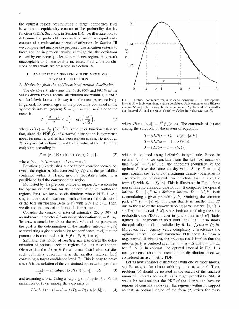
Fig. 1. Optimal confidence region in one-dimensional PDFs. The optimalinterval R = [a, b] containing a given confidence P0 is compared to a differentinterval R′ = [a′, b′] having the same confidence P0. Interval R is smallerthan interval R′, and the value fX(a) = fX(b) fully characterizes R.

where P (x ∈ [a, b]) =∫ b

afX(x) dx. The extremals of (4) are

among the solutions of the system of equations

0 = ∂L/∂λ = P0 − P (x ∈ [a, b]),

0 = ∂L/∂a = −1 + λfX(a),

0 = ∂L/∂b = 1− λfX(b),

which is obtained using Leibniz’s integral rule. Since, ingeneral λ 6= 0, we conclude from the last two equationsthat fX(a) = fX(b), i.e., the endpoints (boundary) of theoptimal R have the same density value. Since R = [a, b]must contain the regions of maximum density (otherwise itssize would not be minimal), we conclude that it is of theform (2) with f0 := fX(a). This is illustrated in Fig. 1 for anon-symmetric unimodal distribution. It compares the optimalinterval R = [a, b] to a different interval R′ = [a′, b′], bothaccumulating a given probability P0. Omitting the commonpart, R ∩ R′ = [a′, b], it is clear that R is smaller than R′

due to the size of the non-overlapping parts: interval [a, a′) issmaller than interval (b, b′], since, both accumulating the sameprobability, the PDF is higher in [a, a′) than in (b, b′] (high-lighted PDF segments in bold solid line). Fig. 1 also showsthe optimality condition satisfied by R, i.e., fX(a) = fX(b).Moreover, such density value completely characterizes theoptimal interval. For any symmetric PDF about its mean µ(e.g. normal distribution), the previous result implies that theinterval [a, b] is centered at µ, i.e., a = µ−∆ and b = µ+∆,for ∆ > 0. In contrast, the optimal interval in Fig. 1 isnot symmetric about the mean of the distribution since weconsidered an asymmetric PDF.

Let us now consider distributions with one or more modes,say Beta(α, β) for almost arbitrary α > 0, β > 0. Then,problem (3) should be restated as the search of the smallestunion of intervals accumulating a target probability. Still, itwould be required that the PDF of the distribution have noregions of constant value (i.e., flat regions) within its supportso that an optimal region of the form (2) exists for every

3

possible value of 0 < P0 < 1. This condition would rule outdistributions such as Beta(α, β) with α = β = 1 (the uniform[0, 1] distribution).

B. Equidensity contours: extremal volume property

We will extend the previous discussion to multiple di-mensions. The next result will prove that, for a broad classof distributions, the optimal region of n-space accumulatinga target confidence level is contained inside an equidensitycontour of the PDF. This is the generalization to multipledimensions of the solution to problem (3).

Result 1. The smallest region R ⊆ Rn containing a targetprobability 0 < P0 < 1 of a distribution whose PDF fX hasno constant regions within its support is given by the interiorof an equidensity contour of the PDF:

R = {x ∈ Rn such that fX(x) ≥ f0}, (5)

where P0 =∫RfX(x)dx and fX(∂R) = f0 at the boundary

of R.

Proof: Let us solve the constrained optimization problem

minR⊂Rn

Vol(R) subject to P (R) = P0, (6)

where Vol(R) =∫Rdx measures the size of R by means of its

volume, the natural measure in Rn, and P (R) =∫RfX(x)dx.

Using a Lagrange multiplier λ ∈ R, the solution of (6) isamong the extremals of

F := Vol(R) + λ (P0 − P (R))

= λP0 +

∫R

(1− λfX(x)) dx.

The extremals satisfy a vanishing necessary optimality con-dition with respect to the variables λ and R. As expected,∂F/∂λ = 0 yields the constraint, P (R) = P0. To computethe sensitivity of F with respect to R, assume that R is a regionvarying smoothly with respect to a parameter t ∈ (−ε, ε), ε >0, R(t) ⊂ Rn, such that R(0) = R is the original region.Then, F also depends on t and, assuming F and dF/dt areboth continuous in an open set containing (−ε, ε), we maycompute dF/dt using Leibniz’s integral rule

d

dt

∫R(t)

g(x, t) dx

=

∫R(t)

∂

∂tg(x, t) dx+

∫B(t)

⟨∂x

∂t(σ), g

(x(σ), t

)N(σ)

⟩dσ,

where g(x, t) ∈ R, B(t) := ∂R(t) is the boundary of R(t),〈x,y〉 is the Euclidean inner product in Rn, N is the out-ward unit normal to B, σ is a local parametrization of B,(∂x/∂t)(σ) is the velocity of the boundary, and dσ is thearea element on B.

In our case, g(x, t) := 1 − λfX(x) does not depend on t,so only the boundary integral (flux) survives in Leibniz’s rule:

dF

dt=

∫B(t)

⟨∂x

∂t(σ), g

(x(σ), t

)N(σ)

⟩dσ.

The first order Taylor expansion of F with respect to t isF ≈ F |t=0 + (dF/dt)|t=0 t. Letting W := ∂x

∂t

∣∣t=0

be the

p1p

2

p3

p4p

5

Optimal (smallest) region R for given P 0

Alternative region R’ for the same P0

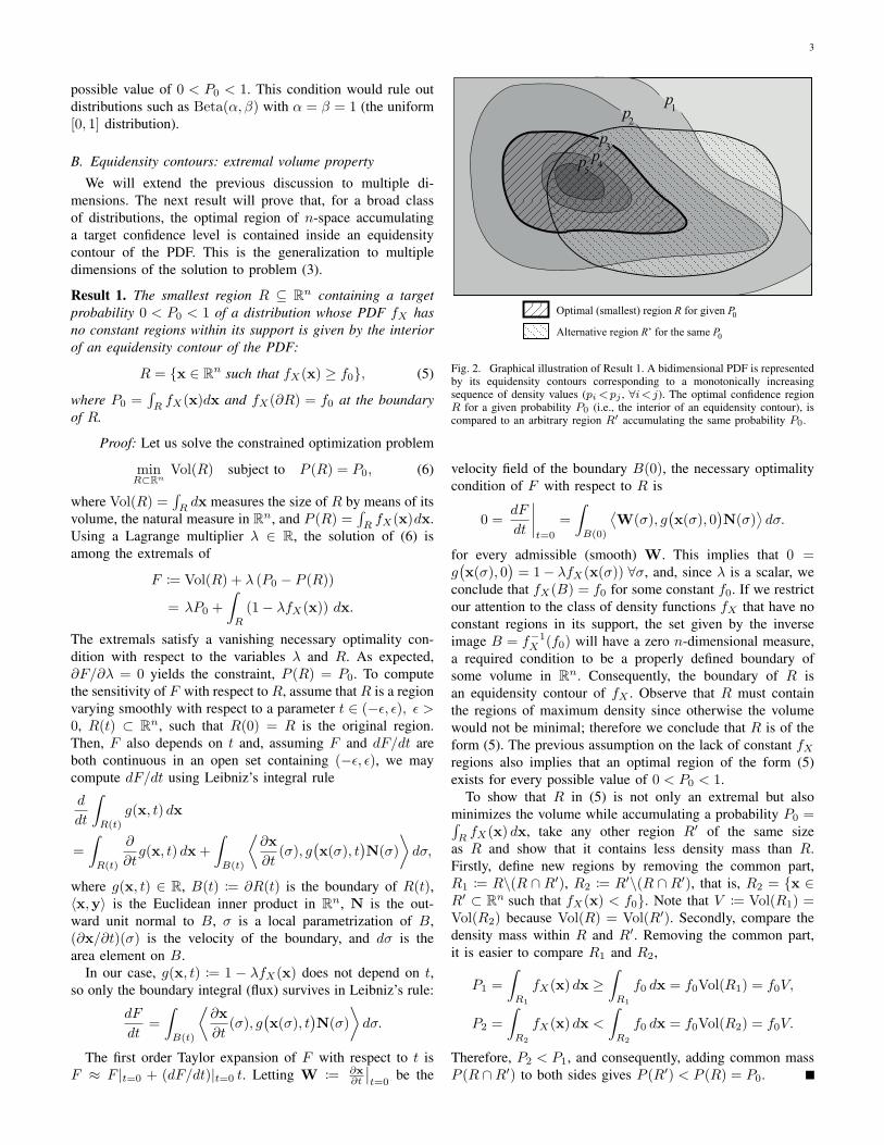
Fig. 2. Graphical illustration of Result 1. A bidimensional PDF is representedby its equidensity contours corresponding to a monotonically increasingsequence of density values (pi<pj , ∀i<j). The optimal confidence regionR for a given probability P0 (i.e., the interior of an equidensity contour), iscompared to an arbitrary region R′ accumulating the same probability P0.

velocity field of the boundary B(0), the necessary optimalitycondition of F with respect to R is

0 =dF

dt

∣∣∣∣t=0

=

∫B(0)

⟨W(σ), g

(x(σ), 0

)N(σ)

⟩dσ.

for every admissible (smooth) W. This implies that 0 =g(x(σ), 0

)= 1− λfX(x(σ)) ∀σ, and, since λ is a scalar, we

conclude that fX(B) = f0 for some constant f0. If we restrictour attention to the class of density functions fX that have noconstant regions in its support, the set given by the inverseimage B = f−1

X (f0) will have a zero n-dimensional measure,a required condition to be a properly defined boundary ofsome volume in Rn. Consequently, the boundary of R isan equidensity contour of fX . Observe that R must containthe regions of maximum density since otherwise the volumewould not be minimal; therefore we conclude that R is of theform (5). The previous assumption on the lack of constant fXregions also implies that an optimal region of the form (5)exists for every possible value of 0 < P0 < 1.

To show that R in (5) is not only an extremal but alsominimizes the volume while accumulating a probability P0 =∫RfX(x) dx, take any other region R′ of the same size

as R and show that it contains less density mass than R.Firstly, define new regions by removing the common part,R1 := R\(R ∩ R′), R2 := R′\(R ∩ R′), that is, R2 = {x ∈R′ ⊂ Rn such that fX(x) < f0}. Note that V := Vol(R1) =Vol(R2) because Vol(R) = Vol(R′). Secondly, compare thedensity mass within R and R′. Removing the common part,it is easier to compare R1 and R2,

P1 =

∫R1

fX(x) dx ≥∫R1

f0 dx = f0Vol(R1) = f0V,

P2 =

∫R2

fX(x) dx <

∫R2

f0 dx = f0Vol(R2) = f0V.

Therefore, P2 < P1, and consequently, adding common massP (R ∩R′) to both sides gives P (R′) < P (R) = P0.

4

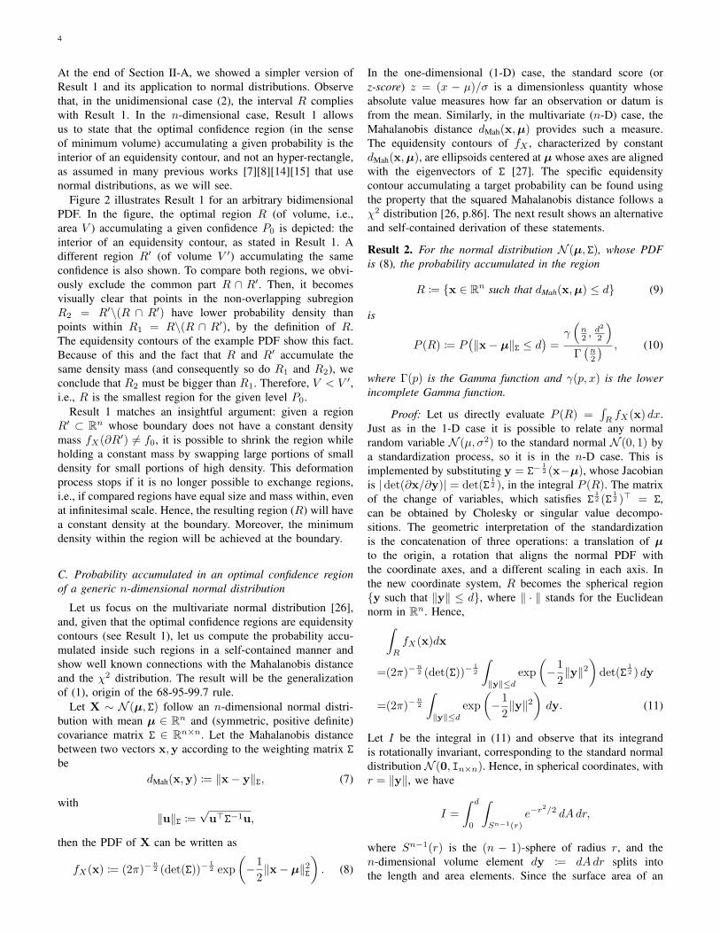
At the end of Section II-A, we showed a simpler version ofResult 1 and its application to normal distributions. Observethat, in the unidimensional case (2), the interval R complieswith Result 1. In the n-dimensional case, Result 1 allowsus to state that the optimal confidence region (in the senseof minimum volume) accumulating a given probability is theinterior of an equidensity contour, and not an hyper-rectangle,as assumed in many previous works [7][8][14][15] that usenormal distributions, as we will see.

Figure 2 illustrates Result 1 for an arbitrary bidimensionalPDF. In the figure, the optimal region R (of volume, i.e.,area V ) accumulating a given confidence P0 is depicted: theinterior of an equidensity contour, as stated in Result 1. Adifferent region R′ (of volume V ′) accumulating the sameconfidence is also shown. To compare both regions, we obvi-ously exclude the common part R ∩ R′. Then, it becomesvisually clear that points in the non-overlapping subregionR2 = R′\(R ∩ R′) have lower probability density thanpoints within R1 = R\(R ∩ R′), by the definition of R.The equidensity contours of the example PDF show this fact.Because of this and the fact that R and R′ accumulate thesame density mass (and consequently so do R1 and R2), weconclude that R2 must be bigger than R1. Therefore, V < V ′,i.e., R is the smallest region for the given level P0.

Result 1 matches an insightful argument: given a regionR′ ⊂ Rn whose boundary does not have a constant densitymass fX(∂R′) 6= f0, it is possible to shrink the region whileholding a constant mass by swapping large portions of smalldensity for small portions of high density. This deformationprocess stops if it is no longer possible to exchange regions,i.e., if compared regions have equal size and mass within, evenat infinitesimal scale. Hence, the resulting region (R) will havea constant density at the boundary. Moreover, the minimumdensity within the region will be achieved at the boundary.

C. Probability accumulated in an optimal confidence regionof a generic n-dimensional normal distribution

Let us focus on the multivariate normal distribution [26],and, given that the optimal confidence regions are equidensitycontours (see Result 1), let us compute the probability accu-mulated inside such regions in a self-contained manner andshow well known connections with the Mahalanobis distanceand the χ2 distribution. The result will be the generalizationof (1), origin of the 68-95-99.7 rule.

Let X ∼ N (µ, Σ) follow an n-dimensional normal distri-bution with mean µ ∈ Rn and (symmetric, positive definite)covariance matrix Σ ∈ Rn×n. Let the Mahalanobis distancebetween two vectors x,y according to the weighting matrix Σ

bedMah(x,y) := ‖x− y‖Σ, (7)

with‖u‖Σ :=

√u>Σ−1u,

then the PDF of X can be written as

fX(x) := (2π)−n2 (det(Σ))−

12 exp

(−1

2‖x− µ‖2Σ

). (8)

In the one-dimensional (1-D) case, the standard score (orz-score) z = (x − µ)/σ is a dimensionless quantity whoseabsolute value measures how far an observation or datum isfrom the mean. Similarly, in the multivariate (n-D) case, theMahalanobis distance dMah(x,µ) provides such a measure.The equidensity contours of fX , characterized by constantdMah(x,µ), are ellipsoids centered at µ whose axes are alignedwith the eigenvectors of Σ [27]. The specific equidensitycontour accumulating a target probability can be found usingthe property that the squared Mahalanobis distance follows aχ2 distribution [26, p.86]. The next result shows an alternativeand self-contained derivation of these statements.

Result 2. For the normal distribution N (µ, Σ), whose PDFis (8), the probability accumulated in the region

R := {x ∈ Rn such that dMah(x,µ) ≤ d} (9)

is

P (R) := P(‖x− µ‖Σ ≤ d

)=

γ(

n2 ,

d2

2

)Γ(n2

) , (10)

where Γ(p) is the Gamma function and γ(p, x) is the lowerincomplete Gamma function.

Proof: Let us directly evaluate P (R) =∫RfX(x) dx.

Just as in the 1-D case it is possible to relate any normalrandom variable N (µ, σ2) to the standard normal N (0, 1) bya standardization process, so it is in the n-D case. This isimplemented by substituting y = Σ−

12 (x−µ), whose Jacobian

is |det(∂x/∂y)| = det(Σ12 ), in the integral P (R). The matrix

of the change of variables, which satisfies Σ12 (Σ

12 )> = Σ,

can be obtained by Cholesky or singular value decompo-sitions. The geometric interpretation of the standardizationis the concatenation of three operations: a translation of µto the origin, a rotation that aligns the normal PDF withthe coordinate axes, and a different scaling in each axis. Inthe new coordinate system, R becomes the spherical region{y such that ‖y‖ ≤ d}, where ‖ · ‖ stands for the Euclideannorm in Rn. Hence,∫

R

fX(x)dx

=(2π)−n2 (det(Σ))−

12

∫‖y‖≤d

exp

(−1

2‖y‖2

)det(Σ

12 ) dy

=(2π)−n2

∫‖y‖≤d

exp

(−1

2‖y‖2

)dy. (11)

Let I be the integral in (11) and observe that its integrandis rotationally invariant, corresponding to the standard normaldistribution N (0, In×n). Hence, in spherical coordinates, withr = ‖y‖, we have

I =

∫ d

0

∫Sn−1(r)

e−r2/2 dAdr,

where Sn−1(r) is the (n − 1)-sphere of radius r, and then-dimensional volume element dy := dAdr splits intothe length and area elements. Since the surface area of an

5

0 1 2 3 4 5 6 70

0.1

0.2

0.3

0.4

0.5

0.6

0.7

0.8

0.9

1

d

P(d

)

n=1n=2n=3n=4n=5n=6n=7n=8n=9n=10n=20n=30

Fig. 3. Curves representing Eq. (10) for n = {1, 2, . . . , 9, 10, 20, 30}. Thethree circular markers illustrate the 68-95-99.7 rule on the curve representingEq. (1).

(n− 1)-sphere of radius r is An−1(r) = r(n−1)An−1(1), withAn−1(1) = 2πn/2/Γ(n/2), substituting t = r2/2, we have

I =

∫ d

0

e−r2/2An−1(r) dr

= An−1(1) 2n2 −1

∫ d2/2

0

tn2 −1e−t dt, (12)

where the last integral is a form of the lower incompleteGamma function

γ(p, x) =

∫ x

0

tp−1 e−t dt. (13)

Collecting results (11), (12) and (13) gives formula (10).The right hand side of (10) coincides with the value of thecumulative distribution function (CDF) of a (centered) chi-squared distribution with n degrees of freedom, χ2

n, for a d2

abscissa, i.e., Fχ2n(d2). This is due to the fact that, after the

standardization, the sum of the squares of n i.i.d. Gaussians isa chi-squared distribution with n degrees of freedom. Hence,as already announced, the squared Mahalanobis distance fol-lows a χ2

n distribution.Equation (10) generalizes (1) to the n-dimensional setting. If

n = 1, the Mahalanobis distance reduces to the z-score (‖x−µ‖Σ = |x−µ|/σ) and, using formulas for special values of theGamma functions, (10) reduces to (1) as expected. Moreover,since γ(p, x) in (13) is a strictly increasing function of x,(10) also establishes a one-to-one correspondence between theregion R (characterized by d > 0 in (9)) and the probabilityit contains, as it is shown in Fig. 3 for different dimensionsn = {1, 2, . . . , 9, 10, 20, 30}. Thus, given a probability value0 < P0 < 1, the value d > 0 that specifies the equidensitycontour bounding the region R for which P0 = P (R) canbe obtained by inverting (10). Scientific software (such as theGNU Scientific Library) provides routines to evaluate the wellknown Gamma functions in (10).

Some special cases deserve further comments. If n is even,the χ2

n distribution coincides with the Erlang distribution ofshape parameter n/2 and scale parameter 2, and (10) admits

further simplifications. In case n = 2, a Rayleigh distribution(of parameter σ = 1) is obtained by taking the square rootof the χ2

2 distribution, i.e., dMah ∼ Rayleigh(1), and a closedform solution exits for d in terms of P : d =

√−2 log(1− P ).

III. COMPARISON OF CLASSIFICATION CRITERIA

While the theory behind (10) should be known to re-searchers and it is properly used in many computer visionworks [28][29][30][31][32], to our surprise, there is a largeamount of works that do not follow such approach. This factmotivates the following analysis of the different incomplete orwrong classification criteria found in the literature.

Table I presents a list of some representative worksamong those using questionable classification criteria to decidewhether a datum matches a multivariate normal distribution.The first four treatises listed in the table (before the doubleline) explicitly provide an erroneous confidence probabilityP , while the rest do not specify such a value (presumablyP ≥ 90%) and therefore use incomplete or inadequate criteria.Most of the references correspond to the specific area ofmoving object detection and take the GMM approach proposedin [13] as a starting point; this is indicated in the secondcolumn of the table. The third column shows the criteriaused in each work (i.e., the shape of the decision/confidenceregions): testing each dimension independently against athreshold (hyper-rectangular regions) or testing the Maha-lanobis distance (7) (ellipsoidal regions). The works that areambiguous about the criterion used are marked with a ‘?’entry. The fourth, fifth and sixth columns contain the followinginformation extracted from the references: the dimension nof the normal model, the distance d considered to build theabovementioned rectangular or ellipsoidal regions, and thetarget confidence probability P . Observe that most cited workshave dimension n = 2, 3 or 5 since they correspond to modelsthat use spatial coordinates and/or the color vector of a pixelas components to apply a distance criterion. The last twocolumns report the actual confidence value (P ) obtained byus resulting from the parameters of the model (informationin columns 3-5). If the criterion (column 3) is clear, only thecorresponding column (Rect. or Ellip.) is given. Otherwise,two confidence values are provided depending on both possibledisambiguations of the criterion.

Table I is further explained in section III-C, but let usdiscuss now the two deceiving situations reported therein:i) the case of choosing hyper-rectangular confidence regionsinstead of ellipsoidal ones (section III-A), and, ii) the caseof choosing an ellipsoidal confidence region of incorrect size(section III-B). Both usual situations arise from misguidedgeneralizations of the familiar unidimensional theory to mul-tiple dimensions.

A. Case I: Treating each dimension independently

Consider an uncorrelated normal distribution N (µ, Σ) withdiagonal covariance matrix Σ = diag(σ2

1 , . . . , σ2n). Let us

compare two classification criteria: a datum x = (xi) ∈ Rn isclassified as a match of the previous distribution if

Criterion 1: dMah(x,µ) ≤ d.

6

TABLE IREFERENCES USING INCOMPLETE OR INADEQUATE CLASSIFICATION CRITERIA.

References Based Criteria n d P (%) P (%)on [13] Rect. Ellip.

2007 Wang et al. [11] Ellip. 3 2.5 98 902009 Li & Prince [10] Ellip. 2 2.5 99 95.62009 Nieto et al. [9] Rect. 2 2.5 99 97.52012 Pedro et al. [33] X Rect. 3 2.5 95 96.3

2000 Stauffer & Grimson [13] X ? 3 2.5 - 96.3 902003 Hayman & Eklundh [14] X Rect. 3 2 - 3 - 86.9 - 99.22003 Zang & Klette [20] X ? 3 2.5 - 96.3 902004 Zivkovic [17] X Ellip. 3 3 - 97.12005 Lee [21] X ? 3 3 - 99.2 97.12005 Jin & Mokhtarian [7] Rect. 3 3 - 99.22006 Luo et al. [8] Rect. 5 3 - 98.72009 Ming et al. [22] X ? 3 2.5 - 96.3 902009 Ying et al. [23] X ? 2 2.5 - 97.5 95.62011 Camplani & Salgado [19] X Ellip. 3 2.5 - 902011 Suhr et al. [15] X Rect. 3 2.5 - 96.32012 Mirabi & Javadi [24] X ? 3 2.5 - 96.3 902012 Gallego et al. [16] X Rect. 3 2.5 - 96.3

0 0.5 1 1.5 2 2.5 3 3.5 40

0.1

0.2

0.3

0.4

0.5

0.6

0.7

0.8

0.9

1

d

P(d

)

n=1n=2n=3n=4n=5n=6n=7n=8n=9n=10n=20n=30

Fig. 4. Curves representing Eq. (14) for n = {1, 2, . . . , 9, 10, 20, 30}. Thethree circular markers illustrate the 68-95-99.7 rule on the curve representingEq. (1). Note the different horizontal axis range with respect to Fig. 3.

Criterion 2: The magnitude of the z-score of each coordi-nate xi of x is smaller than d, i.e., |xi − µi|/σi ≤ dfor i = 1, . . . , n, where µ = (µi) ∈ Rn.

First of all, criterion 2 is meaningless unless the covari-ance matrix Σ of the normal distribution is diagonal (i.e.,the equidensity ellipsoids of the PDF are aligned with thecoordinate axes), whereas criterion 1 is meaningful for anyadmissible covariance Σ. That is why, to compare both criteria,a diagonal Σ was chosen. Also observe that criterion 1 testsa mixture of the coordinates xi against d, whereas criterion 2does not.

Let us compare the confidence regions generated by bothcriteria. For criterion 1,

R1(d) = {x ∈ Rn such that dMah(x,µ) ≤ d}

defines a confidence region with ellipsoidal shape boundedby an equidensity contour since fX(∂R1(d)) = f0. For crite-rion 2, if we define the intervals Ii(d) = {y ∈ R such that |y−

µi|/σi ≤ d} for i = 1, . . . , n, then

R2(d) = {(xi) = x ∈ Rn such that xi ∈ Ii(d)}

is the Cartesian product of the intervals Ii(d), i.e, a hyper-rectangle in Rn, which explains the label ‘Rect.’ in Table I.By virtue of Result 1, confidence regions R2 are not optimalfor normal distributions with n > 1 because they are notthe interior of equidensity contours. Even without Result 1,we may justify the superiority of criterion 1 over criterion 2simply by examining the relationship between both criteriaand the PDF. The value of the normal PDF (8) is a functionof the single parameter dMah. Therefore, any decision that isnot a function of dMah (such as criterion 2) is not taking intoaccount the joint PDF; it is artificially dissociating the decisionfrom the probability density, which is definitely not the desiredgoal.

Even assuming that criterion 2 is valid, although not optimalfor normal distributions, many works in the literature setthe classification threshold d not taking into account thedimensionality n of their models. Let us show how to setsuch a threshold and quantify the classification difference withrespect to criterion 1 by computing the probabilities associatedwith the previous events. For criterion 1, P1 := P (R1(d)) isgiven by (10). For criterion 2,

P2 := P (R2(d)) =

n∏i=1

P (Ii(d)) =

(erf

(d√2

))n

, (14)

which is illustrated in Fig. 4. Obviously, if n = 1, thenP2(d) = P1(d). Comparing Figs. 3 and 4 for n > 1, observethat P1(d) < P2(d) because R1(d) ⊂ R2(d). For n > 1 anda target probability P0 = P1(d1) = P2(d2), we have d2 < d1,but Result 1 guarantees that Vol(R1(d1)) < Vol(R2(d2)), i.e.,the volume of the ellipsoid of “radius” d1 is smaller than thevolume of the hyper-rectangle of sides 2d2σi.

Fig. 5 shows the difference P2 − P1 ≥ 0 between clas-sification criteria. It is stunning that, as the dimension nincreases, the difference can be as large as possible forsome values of d. Typically, based on the z-score for the

7

0 1 2 3 4 5 6 70

0.1

0.2

0.3

0.4

0.5

0.6

0.7

0.8

0.9

1

d

Err

or in

P(d

)

n=1n=2n=3n=4n=5n=6n=7n=8n=9n=10n=20n=30

Fig. 5. Case I. Error curves corresponding to difference of probabilitiesP2 − P1 for n = {1, 2, . . . , 9, 10, 20, 30}. P1 and P2 are represented inFigs. 3 and 4, respectively.

unidimensional distribution, researchers select d ∈ [2, 3]. Fora small dimensionality such as n = 3, this yields moderateerrors of 3% − 12%. However, such deviations can becomedramatic as n increases, for example errors of 15%− 45% ifn = 6, 50% − 68% if n = 10, or even larger, 40% − 95% ifn = 20.

B. Case II: Setting the threshold without taking into accountthe dimension of the model

We concluded in previous sections that the optimal confi-dence region for a normal distribution depends on the Maha-lanobis distance of the datum x from the mean. This sectionanalyzes methods based on this distance, so the covariancematrix does not need to be diagonal in the following discus-sion.

Another common error, more subtle to detect than Case I,is that of setting an incorrect threshold on the Mahalanobisdistance, typically, without taking into account the dimen-sion n of the model. Instead, values drawn from the familiarunidimensional theory (1), e.g., thresholds w ≡ d = {1, 2, 3}corresponding to the 68-95-99.7 rule, are used. The confidenceregions are still ellipsoids, but their Mahalanobis “radius” issmaller than it should be for a target probability. The selectedclassification regions are over-confident [27]: one might thinkthat they accumulate enough probability to reach a desiredconfidence level when in fact they do not because they aresmaller than required.

Fig. 6 shows the errors caused by such a deceiving choiceof classification threshold. For small dimensionality n, theerrors might be small, hence difficult to detect. However, asn increases (for more complicated models), the errors can bearbitrarily large. This is definitely a situation to avoid. Forinstance, a threshold d = 2.5 causes an error of ≈ 10% ifthe model has n = 3, whereas the error grows up to 40%if n = 6, and > 95% if n ≥ 10. In addition, in the typicalinterval d ∈ [2, 3] and for some values of n, there is a wilderror variation. For example, errors of 3% − 23% if n = 3,17% − 64% if n = 6, or 50% − 90% if n = 10. Therefore,

0 1 2 3 4 5 6 70

0.1

0.2

0.3

0.4

0.5

0.6

0.7

0.8

0.9

1

d

Err

or in

P(d

)

n=1n=2n=3n=4n=5n=6n=7n=8n=9n=10n=20n=30

Fig. 6. Case II. Error curves corresponding to difference of probabilitiesP (d; 1)−P (d;n) for n = {1, 2, . . . , 9, 10, 20, 30}. P (d;n) is representedin Fig. 3.

caution is paramount for the selection of the right classificationthreshold depending on the dimensionality of the model n,both to avoid over-confidence (smaller threshold than required)and under-confidence (larger threshold than required).

C. Discussion of confidence regions used in the literature

The works in Table I admit several classifications.According to the sixth column, two categories maybe distinguished: works that provide an incorrect confi-dence level [9][10][11][33], and works that are incom-plete (marked with ‘-’) because they do not specify suchconfidence values. According to the third column, manyworks [20][21][22][23][24] are ambiguous about the clas-sification criterion used. In most cases, this is due to theambiguity inherited from [13]. If the ambiguity is resolved,two interpretations are possible: some treatises [14][16][33]opt for hyper-rectangular regions, while others [17][19] chooseellipsoidal ones. In other references it is not possible to inferthe criteria used, and the choice between both criteria causesconfidence variations, e.g., a 6% variation for the n = 3,d = 2.5 case [13][20][22][24]. The last two columns of Table Iare given taking into account both possible disambiguations.

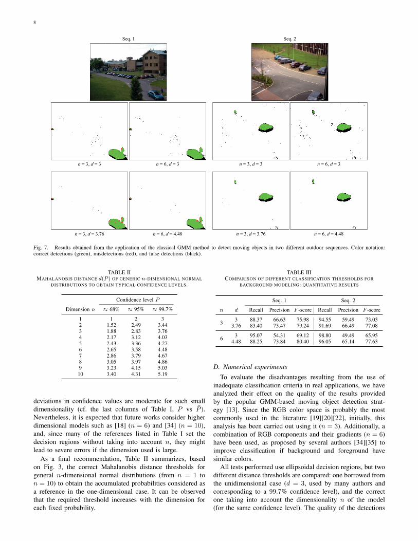
Within classification scenarios, the confidence level thatdetermines the decision regions is usually designed based ona target false detection rate (type I error) of the system, andit therefore also affects the misdetection rate (type II error).Specifically, in moving object detection applications throughbackground modeling ([13] and subsequent works), the twosituations that differ from a nominal confidence design are asfollows. On the one hand, under-confident decision regionscan cause cropped detections and the miss of moving objectswith similar features to those of the background. On the otherhand, over-confident regions improve the detection rate butthey also increase the false alarm rate due to a very restrictivebackground classification.

In [13] and related works, the models are described forarbitrary dimension n, but they are usually exemplified withn = 3 (color components), and, as we have analyzed, the

8

Seq. 1 Seq. 2

n = 3, d = 3 n = 6, d = 3

n = 6, d = 4.48n = 3, d = 3.76

n = 3, d = 3 n = 6, d = 3

n = 3, d = 3.76 n = 6, d = 4.48

Fig. 7. Results obtained from the application of the classical GMM method to detect moving objects in two different outdoor sequences. Color notation:correct detections (green), misdetections (red), and false detections (black).

TABLE IIMAHALANOBIS DISTANCE d(P ) OF GENERIC n-DIMENSIONAL NORMAL

DISTRIBUTIONS TO OBTAIN TYPICAL CONFIDENCE LEVELS.

Confidence level P

Dimension n ≈ 68% ≈ 95% ≈ 99.7%

1 1 2 32 1.52 2.49 3.443 1.88 2.83 3.764 2.17 3.12 4.035 2.43 3.36 4.276 2.65 3.58 4.487 2.86 3.79 4.678 3.05 3.97 4.869 3.23 4.15 5.03

10 3.40 4.31 5.19

deviations in confidence values are moderate for such smalldimensionality (cf. the last columns of Table I, P vs P ).Nevertheless, it is expected that future works consider higherdimensional models such as [18] (n = 6) and [34] (n = 10),and, since many of the references listed in Table I set thedecision regions without taking into account n, they mightlead to severe errors if the dimension used is large.

As a final recommendation, Table II summarizes, basedon Fig. 3, the correct Mahalanobis distance thresholds forgeneral n-dimensional normal distributions (from n = 1 ton = 10) to obtain the accumulated probabilities considered asa reference in the one-dimensional case. It can be observedthat the required threshold increases with the dimension foreach fixed probability.

TABLE IIICOMPARISON OF DIFFERENT CLASSIFICATION THRESHOLDS FOR

BACKGROUND MODELING: QUANTITATIVE RESULTS

Seq. 1 Seq. 2

n d Recall Precision F -score Recall Precision F -score

3 3 88.37 66.63 75.98 94.55 59.49 73.033.76 83.40 75.47 79.24 91.69 66.49 77.08

6 3 95.07 54.31 69.12 98.80 49.49 65.954.48 88.25 73.84 80.40 96.05 65.14 77.63

D. Numerical experiments

To evaluate the disadvantages resulting from the use ofinadequate classification criteria in real applications, we haveanalyzed their effect on the quality of the results providedby the popular GMM-based moving object detection strat-egy [13]. Since the RGB color space is probably the mostcommonly used in the literature [19][20][22], initially, thisanalysis has been carried out using it (n = 3). Additionally, acombination of RGB components and their gradients (n = 6)have been used, as proposed by several authors [34][35] toimprove classification if background and foreground havesimilar colors.

All tests performed use ellipsoidal decision regions, but twodifferent distance thresholds are compared: one borrowed fromthe unidimensional case (d = 3, used by many authors andcorresponding to a 99.7% confidence level), and the correctone taking into account the dimensionality n of the model(for the same confidence level). The quality of the detections

9

provided by the analyzed method is measured by meansof the conventional recall, precision and F -score evaluationparameters [36].

Figure 7 illustrates some of the results obtained for twooutdoor sequences from the PETS database [37], and Table IIIreports the corresponding quality measurements. It can beobserved that the background variations are better capturedusing the adequate classification thresholds (d = 3.76 if n = 3or d = 4.48 if n = 6) than in case of the fixed threshold takenfrom the unidimensional case (d = 3, over-confident region):the amount of false detections is significantly reduced in allthe analyzed cases, and consequently, the overall quality ofthe detections (given by the F -score) is clearly improved. Thisquality improvement is more noticeable as model dimension-ality increases.

IV. CONCLUSION

In this work, we have provided a detailed comparativeanalysis between the correct confidence regions correspondingto general multidimensional normal distributions and certainincomplete and/or erroneous but frequent practices observedin the literature.

To this end, we have studied general n-dimensional prob-ability distributions and have proved that, for a broad classof them, the optimal confidence region accumulating a targetconfidence level is the interior of an equidensity contour of thePDF. For multivariate normal distributions, the Mahalanobisdistance provides the right dimensionless quantity (fully char-acterizing the equidensity contours of the PDF) for decisionmaking, i.e., for establishing confidence regions. Hence, deci-sions based on individual z-scores (one per dimension), whichlead to hyper-rectangular confidence regions, are discouraged.

We have derived the formula that relates the size of anoptimal confidence region (specified by its largest Mahalanobisdistance) and its cumulated probability. Concisely, the squaredMahalanobis distance follows a Chi-squared distribution withn degrees of freedom. We used this formula to quantify theerrors harvested by many works in the literature, mostly causedby a wrong extrapolation of unidimensional results withouttaking into account the dimensionality of the model. Usingseveral plots, we showed that such errors can be significantlylarge depending on the dimension n. In particular, we dis-cussed the deviations in the typical threshold range d ∈ [2, 3].

To prevent errors from propagating to future works, we havespecified the correct threshold values that describe the optimalconfidence regions for some common target confidence levels.Finally, we have demonstrated the theoretical analysis with aconcrete example in the context of moving object detection.

REFERENCES

[1] P. Larranaga, H. Karshenas, C. Bielza, and R. Santana, “A review onprobabilistic graphical models in evolutionary computation,” Journal ofHeuristics, pp. 1–25, 2012.

[2] E. Chen, O. Haik, and Y. Yitzhaky, “Classification of moving objects inatmospherically degraded video,” Optical Engineering, vol. 51, no. 10,pp. 101 710–1, 2012.

[3] M. Kristan, A. Leonardis, and D. Skocaj, “Multivariate online kerneldensity estimation with Gaussian kernels,” Pattern Recognition, vol. 44,no. 10, pp. 2630–2642, 2011.

[4] A. Elgammal, R. Duraiswami, D. Harwood, and L. Davis, “Backgroundand foreground modeling using nonparametric kernel density estimationfor visual surveillance,” Proceedings of the IEEE, vol. 90, no. 7, pp.1151–1163, 2002.

[5] C. Cuevas, D. Berjon, F. Moran, and N. Garcıa, “Moving objectdetection for real-time augmented reality applications in a GPGPU,”IEEE Trans. Consumer Electronics, vol. 58, no. 1, pp. 117–125, 2012.

[6] T. Huang, X. Fang, J. Qiu, and T. Ikenaga, “Adaptively adjustedGaussian mixture models for surveillance applications,” Advances inMultimedia Modeling, pp. 689–694, 2010.

[7] Y. Jin and F. Mokhtarian, “Towards robust head tracking by particles,”in IEEE Int. Conf. Image Processing, vol. 3, 2005, pp. 864–867.

[8] X. Luo, S. Bhandarkar, W. Hua, and H. Gu, “Nonparametric backgroundmodeling using the CONDENSATION algorithm,” in IEEE Int. Conf.Video and Signal Based Surveillance, 2006, pp. 1–6.

[9] M. Nieto, C. Cuevas, and L. Salgado, “Measurement-based reclusteringfor multiple object tracking with particle filters,” in IEEE Int. Conf.Image Processing, 2009, pp. 4097–4100.

[10] P. Li and S. Prince, “Joint and implicit registration for face recognition,”in IEEE Conf. Computer Vision and Pattern Recognition, 2009, pp.1510–1517.

[11] H. Wang, D. Suter, K. Schindler, and C. Shen, “Adaptive object trackingbased on an effective appearance filter,” IEEE Trans. Pattern Analysisand Machine Intelligence, vol. 29, no. 9, pp. 1661–1667, 2007.

[12] H. Hassanpour, M. Sedighi, and A. Manashty, “Video frame’s back-ground modeling: Reviewing the techniques,” Journal of Signal andInformation Processing, vol. 2, no. 2, pp. 72–78, 2011.

[13] C. Stauffer and W. Grimson, “Learning patterns of activity using real-time tracking,” IEEE Trans. Pattern Analysis and Machine Intelligence,vol. 22, no. 8, pp. 747–757, 2000.

[14] E. Hayman and J.-O. Eklundh, “Statistical background subtraction for amobile observer,” in Int. Conf. Computer Vision, 2003, pp. 67–74 vol.1.

[15] J. Suhr, H. Jung, G. Li, and J. Kim, “Mixture of Gaussians-basedbackground subtraction for bayer-pattern image sequences,” IEEE Trans.Circuits and Systems for Video Technology, vol. 21, no. 3, pp. 365–370,2011.

[16] J. Gallego, M. Pardas, and G. Haro, “Enhanced foreground segmentationand tracking combining Bayesian background, shadow and foregroundmodeling,” Pattern Recognition Letters, vol. 33, no. 12, pp. 1558–1568,2012.

[17] Z. Zivkovic, “Improved adaptive Gaussian mixture model for back-ground subtraction,” in IEEE Int. Conf. Pattern Recognition, vol. 2, 2004,pp. 28–31.

[18] Q. Wan and Y. Wang, “Background subtraction based on adaptivenon-parametric model,” in World Congress on Intelligent Control andAutomation., 2008, pp. 5960–5965.

[19] M. Camplani and L. Salgado, “Adaptive background modeling in mul-ticamera system for real-time object detection,” Optical Engineering,vol. 50, no. 12, pp. 127 206:1–17, 2011.

[20] Q. Zang and R. Klette, “Evaluation of an adaptive composite Gaussianmodel in video surveillance,” in Computer Analysis of Images andPatterns. Springer, 2003, pp. 165–172.

[21] D. Lee, “Effective Gaussian mixture learning for video backgroundsubtraction,” IEEE Trans. Pattern Analysis and Machine Intelligence,vol. 27, no. 5, pp. 827–832, 2005.

[22] Y. Ming, C. Guodong, and Q. Lichao, “Player detection algorithm basedon Gaussian mixture models background modeling,” in IEEE Int. Conf.Intelligent Networks and Intelligent Systems, 2009, pp. 323–326.

[23] L. Ying-hong, X. Chang-zhen, Y. Yi-xin, and L. Ya-li, “Moving objectdetection based on edged mixture Gaussian models,” in IEEE Int.Workshop on Intelligent Systems and Applications, 2009, pp. 1–5.

[24] M. Mirabi and S. Javadi, “People tracking in outdoor environment usingKalman filter,” in IEEE Int. Conf. Intelligent Systems, Modelling andSimulation, 2012, pp. 303–307.

[25] A. Papoulis and U. S. Pillai, Probability, Random Variables and Stochas-tic Processes. McGraw-Hill, 2002.

[26] A. C. Rencher, Methods of Multivariate Analysis, ser. Wiley Series inProbability and Statistics. Wiley, 2003.

[27] R. Blanc, E. Syrkina, and G. Szekely, “Estimating the Confidence ofStatistical Model Based Shape Prediction,” in Information Processingin Medical Imaging. Springer, 2009, vol. 5636, LNCS, pp. 602–613.

[28] C. Schmid and R. Mohr, “Combining greyvalue invariants with localconstraints for object recognition,” in IEEE Int. Conf. Computer Visionand Pattern Recognition, 1996, pp. 872–877.

[29] K. Arras and S. Vestli, “Hybrid, high-precision localisation for the maildistributing mobile robot system MOPS,” in IEEE Int. Conf. Roboticsand Automation, vol. 4, 1998, pp. 3129–3134.

10

[30] M. Dissanayake, P. Newman, S. Clark, H. Durrant-Whyte, andM. Csorba, “A solution to the simultaneous localization and mapbuilding (SLAM) problem,” IEEE Trans. Robotics and Automation,vol. 17, no. 3, pp. 229–241, 2001.

[31] Z. Guo, G. Jiang, H. Chen, and K. Yoshihira, “Tracking probabilisticcorrelation of monitoring data for fault detection in complex systems,” inIEEE Int. Conf. Dependable Systems and Networks, 2006, pp. 259–268.

[32] D. Won, H. Oh, S. Huh, D. Shim, and M. Tahk, “Multiple UAVs trackingalgorithm with a multi-camera system,” in IEEE Int. Conf. ControlAutomation and Systems (ICCAS), 2010, pp. 2357–2360.

[33] L. Pedro, G. A. Caurin, V. Belini, R. Pechoneri, A. Gonzaga, I. Neto,F. Nazareno, and M. Stucheli, “Hand gesture recognition for robot handteleoperation,” in ABCM Symposium Series in Mechatronics, vol. 5,2012, pp. 1065–1074.

[34] C. Cuevas and N. Garcıa, “Tracking-based non-parametric background-foreground classification in a chromaticity-gradient space,” in IEEE Int.Conf. Image Processing, 2010, pp. 845–848.

[35] S. Atev, O. Masoud, and N. Papanikolopoulos, “Practical mixturesof gaussians with brightness monitoring,” in Intelligent TransportationSystems, 2004. Proceedings. The 7th International IEEE Conference on.IEEE, 2004, pp. 423–428.

[36] F.-C. Cheng and S.-J. Ruan, “Accurate motion detection using a self-adaptive background matching framework,” Intelligent TransportationSystems, IEEE Transactions on, vol. 13, no. 2, pp. 671–679, 2012.

[37] Computational Vision Group, “PETS: Performance Evaluation of Track-ing and Surveillance,” http://www.cvg.rdg.ac.uk/, University of Reading.

Guillermo Gallego received the Ingeniero de Tele-comunicacion degree (five years engineering pro-gram) from the Universidad Politecnica de Madrid,Spain, in 2004, M.S. degree in mathematical engi-neering (Magıster en Ingenierıa Matematica) fromthe Universidad Complutense de Madrid, Madrid, in2005, and the M.S. in electrical and computer engi-neering, M.S. in mathematics, and Ph.D. in electricaland computer engineering from the Georgia Instituteof Technology, Atlanta, in 2007, 2009 and 2011,respectively.

He was a recipient of the Fulbright Scholarship to pursue graduate studies atthe Georgia Institute of Technology in 2005. Since 2011, he has been a Marie-Curie COFUND post-doctoral researcher with the Universidad Politecnicade Madrid. His research interests fall within the areas of signal processing,geometry, optimization, computer vision and ocean engineering.

Carlos Cuevas received the Ingeniero de Teleco-municacion degree (integrated BSc-MSc accreditedby ABET) in 2006 and the Doctor Ingeniero deTelecomunicacin degree (Ph.D. in Communications),in 2011, both from the Universidad Politecnica deMadrid (UPM), Madrid, Spain.

Since 2006 he has been a member of the Grupo deTratamiento de Imagenes (Image Processing Group)of the UPM. His research interests include signal andimage processing, computer vision, pattern recogni-tion and automatic target recognition.

Raul Mohedano received the Ingeniero de Teleco-municacion degree (five years engineering program)in 2006 from the Universidad Politecnica de Madrid(UPM), Madrid, Spain.

Since 2007 he has been a member of the Grupo deTratamiento de Imagenes (Image Processing Group)of the UPM, where he holds a personal researchgrant from the Comunidad de Madrid. His researchinterests are in the area of computer vision.

Narciso Garcıa received the Ingeniero de Tele-comunicacion degree (five years engineering pro-gram) in 1976 (Spanish National Graduation Award)and the Doctor Ingeniero de Telecomunicacion de-gree (Ph.D. in Communications) in 1983 (Doc-toral Graduation Award), both from the UniversidadPolitecnica de Madrid (UPM), Madrid, Spain.

Since 1977 he is a faculty member with theUPM where he is currently a Professor of SignalTheory and Communications. He leads the Grupo deTratamiento de Imagenes (Image Processing Group)

of the UPM. He has been actively involved in Spanish and European researchprojects, serving also as evaluator, reviewer, auditor, and observer of severalresearch and development programmes of the European Union. He was a co-writer of the EBU proposal, basis of the ITU standard for digital transmissionof TV at 34-45 Mb/s (ITU-T J.81). His professional and research interestsare in the areas of digital image processing, video compression and computervision.