On the Mechanism of Urea-Induced Protein Denaturation

Matteus Lindgren

Department of Chemistry

901 87 Umeå Umeå 2010 Sweden

Copyright©Matteus Lindgren, 2010 ISBN: 978-91-7264-997-2 Printed by: VMC KBC Umeå, Sweden 2010

Nobody climbs mountains for scientific reasons. Science is used to raise

money for the expeditions, but you really climb for the hell of it.

Edmund Hillary

Table of Contents

List of Papers 1

Abstract 2

1. Project Description 3

2. Methods

2.1. Molecular Dynamics Simulations 8

2.2. Nuclear Magnetic Resonance Spectroscopy 18

3. The Research Field of Chemical Denaturation

3.1. The Thermodynamics of Protein – Urea Systems 26

3.2. Proposed Mechanisms of Urea-Induced Denaturation 31

3.3. MD Simulation Studies of Chemical Denaturation 34

4. Results 37

5. Discussion 42

6. My View of the Mechanism of Urea 45

Acknowledgments 47

References 49

1

List of Papers

This thesis is based on the following papers, which are referred to in the text by the Roman numerals I-III. The papers can be found as reprints at the end of the thesis.

I. M. Lindgren, P.-O. Westlund

On the stability of Chymotrypsin Inhibitor 2 in a 10 M urea solution. The role of interaction energies for urea-induced protein denaturation.

Accepted for publication in Phys. Chem. Chem. Phys.

II. M. Lindgren, T. Sparrman, P.-O. Westlund

A combined molecular dynamic simulation and urea 14N NMR

relaxation study of the urea-lysozyme system

Spectrochimica Acta Part A, 2010, 75, 953

III. M. Lindgren, P.-O. Westlund

The affect of urea on the kinetics of local unfolding processes in

Chymotrypsin Inhibitor 2

Submitted to Biophysical Chemistry

2

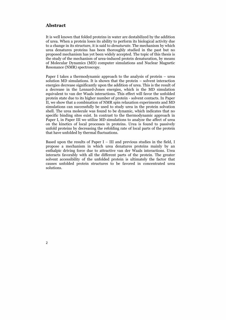
Abstract

It is well known that folded proteins in water are destabilized by the addition of urea. When a protein loses its ability to perform its biological activity due to a change in its structure, it is said to denaturate. The mechanism by which urea denatures proteins has been thoroughly studied in the past but no proposed mechanism has yet been widely accepted. The topic of this thesis is the study of the mechanism of urea-induced protein denaturation, by means of Molecular Dynamics (MD) computer simulations and Nuclear Magnetic Resonance (NMR) spectroscopy.

Paper I takes a thermodynamic approach to the analysis of protein – urea solution MD simulations. It is shown that the protein – solvent interaction energies decrease significantly upon the addition of urea. This is the result of a decrease in the Lennard-Jones energies, which is the MD simulation equivalent to van der Waals interactions. This effect will favor the unfolded protein state due to its higher number of protein - solvent contacts. In Paper II, we show that a combination of NMR spin relaxation experiments and MD simulations can successfully be used to study urea in the protein solvation shell. The urea molecule was found to be dynamic, which indicates that no specific binding sites exist. In contrast to the thermodynamic approach in Paper I, in Paper III we utilize MD simulations to analyze the affect of urea on the kinetics of local processes in proteins. Urea is found to passively unfold proteins by decreasing the refolding rate of local parts of the protein that have unfolded by thermal fluctuations.

Based upon the results of Paper I – III and previous studies in the field, I propose a mechanism in which urea denatures proteins mainly by an enthalpic driving force due to attractive van der Waals interactions. Urea interacts favorably with all the different parts of the protein. The greater solvent accessibility of the unfolded protein is ultimately the factor that causes unfolded protein structures to be favored in concentrated urea solutions.

3

1. Project Description

Proteins are the machines of living organisms. They are responsible for the

construction, the maintenance and the degradation of the cells constituting

the organism, but they are also involved in the communication and transport

of substances between the cells. Proteins are long molecular chains of

covalently bonded units called amino acids. The genetic code incorporated

into the DNA molecule includes information about the sequence of amino

acids that are to be linked together in order to produce a specific protein.

However, for the protein to be able to perform its biological function, a

specific structure and the right amount of structural flexibility needs to be

incorporated, in addition to the correct sequence of amino acids. The process

when a protein undergoes a transition from the unstructured polymer to a

compact three-dimensional structure is termed protein folding. The

structure that the protein adopts is determined by the chemical and physical

properties of its inherent amino acids in combination with the local

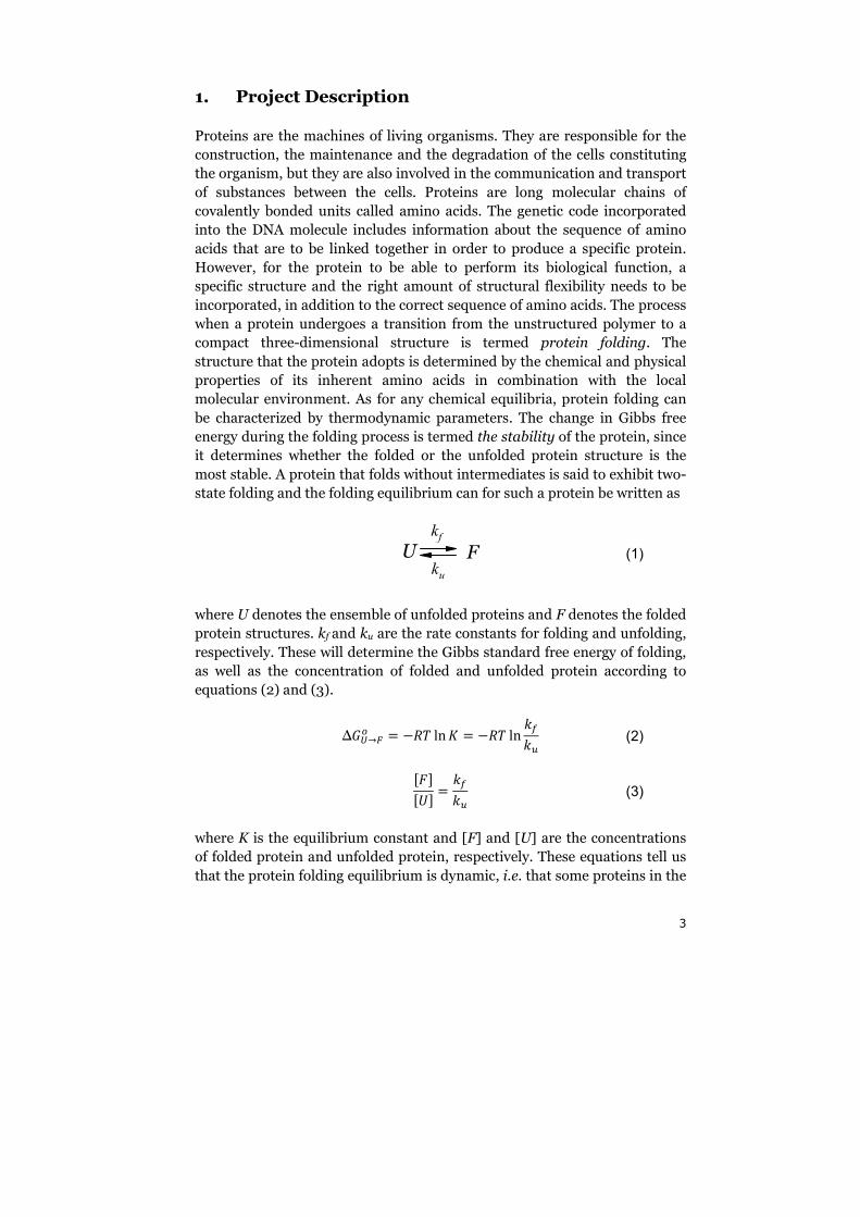
molecular environment. As for any chemical equilibria, protein folding can

be characterized by thermodynamic parameters. The change in Gibbs free

energy during the folding process is termed the stability of the protein, since

it determines whether the folded or the unfolded protein structure is the

most stable. A protein that folds without intermediates is said to exhibit two-

state folding and the folding equilibrium can for such a protein be written as

U Fku

kf

(1)

where U denotes the ensemble of unfolded proteins and F denotes the folded

protein structures. kf and ku are the rate constants for folding and unfolding,

respectively. These will determine the Gibbs standard free energy of folding,

as well as the concentration of folded and unfolded protein according to

equations (2) and (3).

∆����� � �� ln � � �� ln � � (2)

������ � � � (3)

where K is the equilibrium constant and [F] and [U] are the concentrations

of folded protein and unfolded protein, respectively. These equations tell us

that the protein folding equilibrium is dynamic, i.e. that some proteins in the

4

sample will fold while others unfold at the same time. The equilibrium

concentrations of the folded and the unfolded species are reached when they

match the rates of conversion from one species to the other. It is therefore

equally valid to consider the unfolding reaction as being the forward

reaction, i.e. we consider the reaction

F U

ku

kf

(4)

for which the Gibbs standard free energy can be written as:

∆����� � �� ln � � � �∆����� (5)

A protein that exhibits two-state folding and unfolding has a relatively

smooth free energy landscape with only two dominating minima along the

folding pathway. The free energy barrier that separates the two minima

corresponds to a transition state (TS) protein structure. Transition state

theory allows us to connect the relative height of the barrier versus the two minima, ∆������ and ∆������ , with the rate constants � and �:

� � � �� exp ��∆������� � (6)

� � � �� exp ��∆������� � (7)

where �, � and � is the transmission coefficient, Boltzmann´s constant and

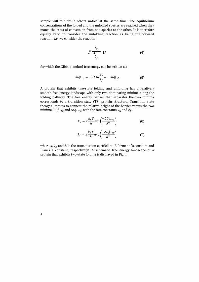
Planck´s constant, respectively1. A schematic free energy landscape of a

protein that exhibits two-state folding is displayed in Fig. 1.

5

Fig. 1. Schematic free energy landscape of a protein in water that exhibits two-state folding. The

reaction coordinate ζ represents the averaged folding / unfolding pathway.

The equilibrium between the folded and the unfolded protein structures will

be governed by the interplay between protein – protein interactions, solvent

– solvent interactions and protein – solvent interactions. Folding of a

protein increases the number of protein – protein contacts and solvent –

solvent contacts. Unfolding on the other hand increases the solvent

accessible surface area of the protein and therefore the number of protein –

solvent contacts. If the interactions between the protein and the solvent are

more favorable (in a general sense), the dominating protein structure will be

the unfolded form, rather than the folded form. The stability of a folded

protein depends upon several factors, such as the type of solvent, the pH, the

ionic strength and the temperature. It has been known for a century that the

addition of urea, H2N-CO-NH2, to a protein – water solution destabilizes the

folded protein structure2. The unfolded protein structures dominate at high

urea concentrations for all but the most stable proteins. When a protein loses

its ability to perform its biological activity due to a change in its structure, it

is said to denaturate. Urea is therefore called a denaturant. Urea is by no

means the only substance that can destabilize proteins3. Another well-known

denaturant is the salt guanidinium chloride. Other molecules, such as

trimethylamine N-oxide (TMAO), have a large stabilizing effect on proteins.

The research field of chemical denaturation incorporates all denaturants

and their effect on proteins.

6

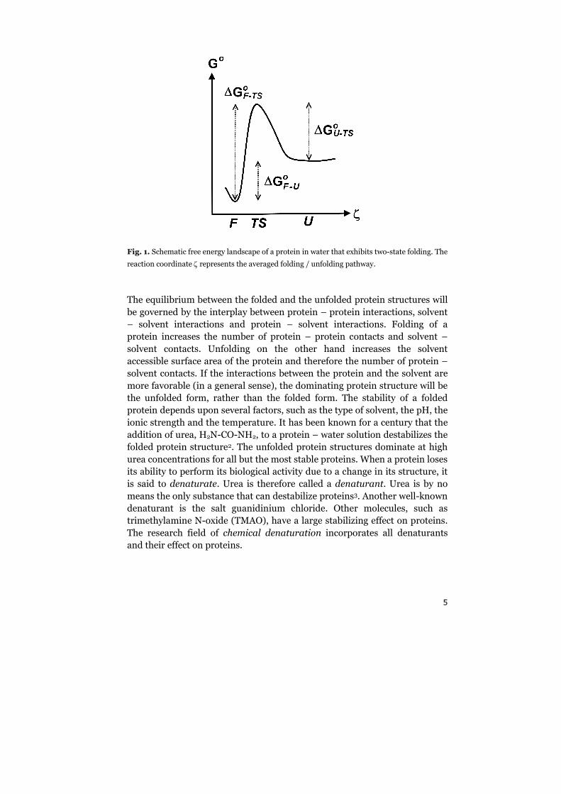
When urea is added, the unfolding free energy decreases, from a positive

value to a negative value at high concentrations. Stopped flow studies, see for

example Ref. 4, have shown that the unfolding free energy is decreased in

urea solutions by means of an increased unfolding rate while the folding rate

decreases by approximately the same amount, but the exact behavior

depends upon the type of protein. This means that ∆������ is decreased and ∆������ is increased in the presence of urea. The change of the unfolding free

energy landscape due to urea is schematically shown in Fig. 2.

Fig. 2. Schematic free energy landscape that shows the affect of urea on the relative barrier

heights of a protein. Note that the absolute height of the barrier may also be changed by urea

but it is assumed to be unchanged in this figure.

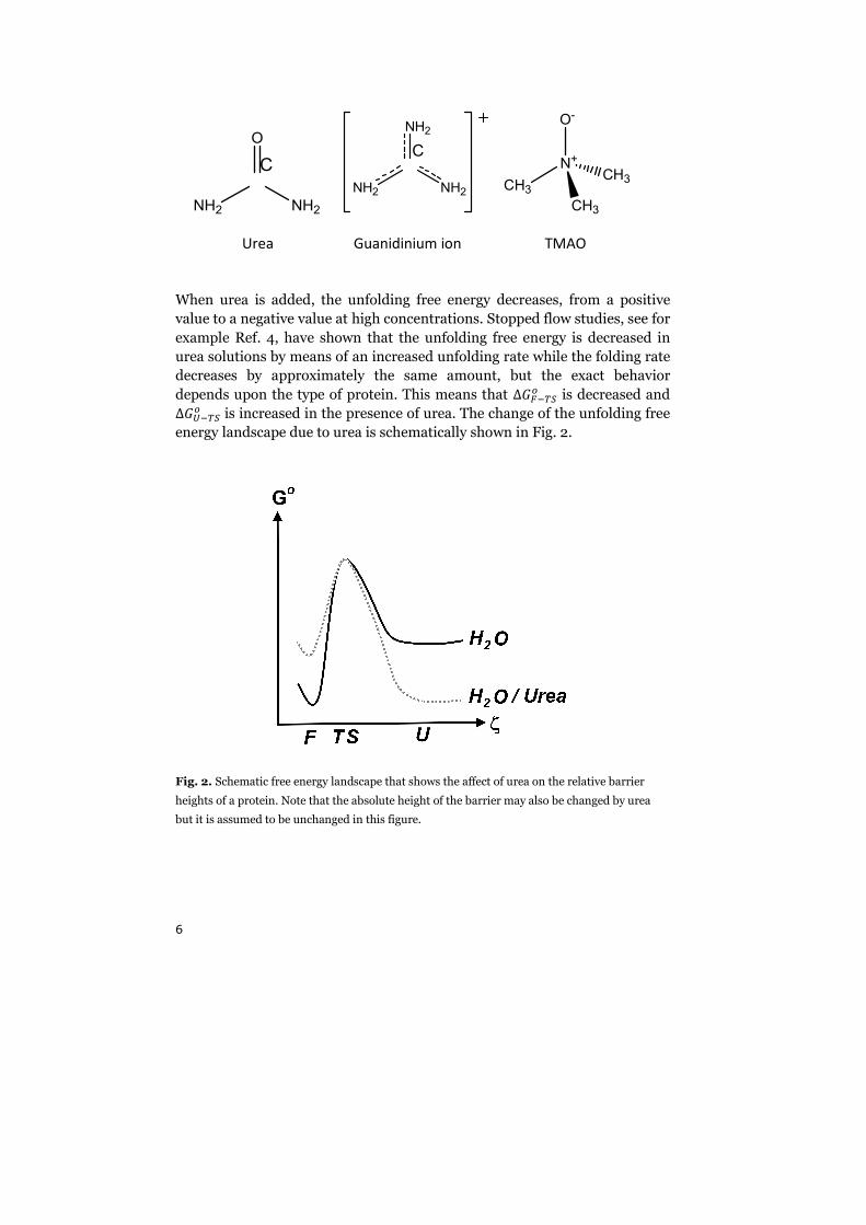
C

O

NH2NH2

C

NH2

NH2NH2

N+

O-

CH3CH3

CH3

Urea Guanidinium ion TMAO

7

Motivation for the project

Urea has a very widespread use in laboratory experiments due to its ability to

unfold proteins without reacting with the proteins. Urea is for example used

in protein folding research as well as in studies concerning the effect of

mutations on the protein properties. The extensive use of urea in research

creates a need to understand the mechanism by which urea destabilizes

proteins. Urea solutions have also gained attention due to the general

importance of understanding how the interactions between a protein and its

chemical environment affect the structure and the dynamics of the protein.

The research field of chemical denaturation has therefore been extensively

studied both in the past and at present. However, the mechanism of urea-

induced denaturation is still not known in detail.

Aim of the project

The aim was to study the effects of urea on water and on proteins in order to

retrieve information regarding urea-induced denaturation.

8

2. Methods

2.1. Molecular Dynamics Simulations

The first scientific work utilizing Molecular Dynamics (MD) computer

simulations was published in 19575. Even though five decades have passed,

their description of the method of MD simulations still applies: “The method

consists of solving exactly (to the number of significant figures carried) the

simultaneous classical equations of motion of several hundred particles by

means of fast electronic computors.” However, due to the dramatically

increased computer performance during the years that have since passed,

the scale of the systems that are possible to study has now increased from

several hundred particles and 200 000 collisions to 100 000 atoms and

micro seconds of simulation time. MD simulations are now routinely used in

research involving molecular systems6. Not only the hardware but also the

software has evolved. A number of sophisticated MD simulation software

suites are now available. Arguably, the programs most commonly used in

research of biomolecules are CHARMM7, AMBER8, GROMACS9, ENCAD10

and NAMD11.

MD simulations are based upon classical mechanics, in contrast to

simulations utilizing a varying degree of quantum mechanical theories. The

advantage is the lower computational cost and therefore the ability to study

phenomena taking place on a longer time scale and/or larger systems. The

disadvantage is that electrons cannot be explicitly treated. This limits MD

simulations to studies without chemical reactions. In addition, the accuracy

of the simulations depends on how well the quantum mechanical energy

landscape can be approximated by an effective potential, governed by the

laws of classical physics. For a system consisting of N particles, the core of

the MD simulation algorithm consists of solving Newton´s equation of

motion for an N particle system:

! "#$%"&# � '% , ( � 1 … + (8)

The forces '% are the gradient of the potential energy �,$-,$#, … $./

'% � � 1�2$%31$%

(9)

When the force acting on each particle has been acquired at a specific time t,

numerical integration of the equations of motion yields new particle

positions at a time (t + ∆t). However, several algorithms are available for the

9

integration. Based on a Taylor expansion of the positions at time t, the Euler

algorithm in Eq. (10) seems to be the natural choice.

$%2& 4 ∆&3 � $%2&3 4 5%2&3∆& 4 '%2&32!% 2∆&3# (10)

where 5% is the velocity of particle i. Unfortunately, the Euler algorithm has

some inherent problems. For example, it is not time reversible and it also

suffers from a large energy drift. It is therefore common to use other

algorithms, such as the Verlet algorithm, the velocity Verlet algorithm or the

Leap-Frog algorithm. The Leap-Frog algorithm constitutes Eq. (11) and (12)

12.

$%2& 4 ∆&3 � $%2&3 4 57 8& 4 ∆&2 9 ∆& (11)

57 8& 4 ∆&2 9 � 57 8& � ∆&2 9 4 '7!% ∆& (12)

MD simulations commonly utilize pair-potentials, i.e. the potential energy

and the force of each particle in the system is calculated by a sum of two-

particle interactions. In order to calculate the potential energy for a given set

of particle coordinates, one must first define the set of equations describing

the different interactions that occur in the system, i.e. the force field must be

defined. The most common type of force field utilized in MD simulations of

biomolecules is the Class I type. The terms included in this force field are

common among the most widely used MD simulation programs such as

CHARMM, AMBER and GROMACS. An example of a Class I potential

energy function is displayed in Eq. (13) - (15).

� � �:;<=>= 4 �<;<�:;<=>=

(13)

�:;<=>= � ? �:2@ � @A3#:;<=B4 ? �C2D � DA3#

E<FG>B4 ? �H21 4 cos2LM � N33=%O>=PEGB4 ? �%QR2S � SA3#%QRP;R>PB

(14)

10

�<;<�:;<=>= � 12 ? ? T4V%W X�Y%W@%W �-# � �Y%W@%W �Z[ 4 \%\W4]V@%W^W_%%

(15)

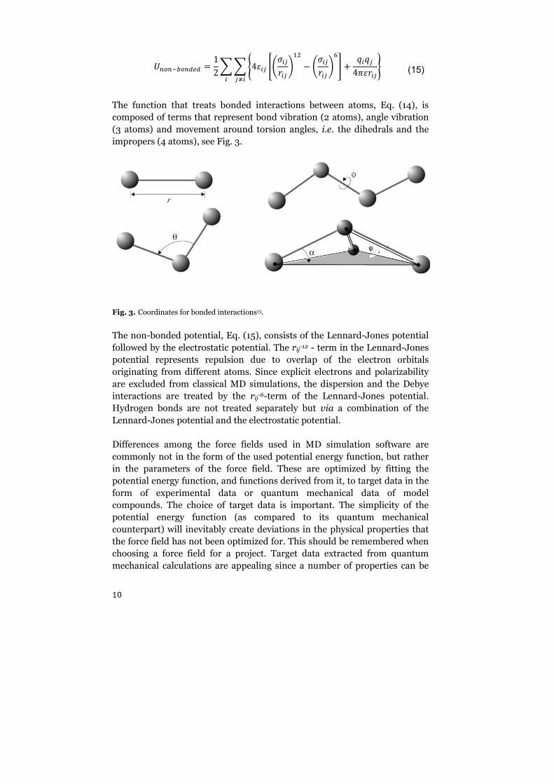
The function that treats bonded interactions between atoms, Eq. (14), is

composed of terms that represent bond vibration (2 atoms), angle vibration

(3 atoms) and movement around torsion angles, i.e. the dihedrals and the

impropers (4 atoms), see Fig. 3.

Fig. 3. Coordinates for bonded interactions13.

The non-bonded potential, Eq. (15), consists of the Lennard-Jones potential

followed by the electrostatic potential. The rij-12 - term in the Lennard-Jones

potential represents repulsion due to overlap of the electron orbitals

originating from different atoms. Since explicit electrons and polarizability

are excluded from classical MD simulations, the dispersion and the Debye

interactions are treated by the rij-6-term of the Lennard-Jones potential.

Hydrogen bonds are not treated separately but via a combination of the

Lennard-Jones potential and the electrostatic potential.

Differences among the force fields used in MD simulation software are

commonly not in the form of the used potential energy function, but rather

in the parameters of the force field. These are optimized by fitting the

potential energy function, and functions derived from it, to target data in the

form of experimental data or quantum mechanical data of model

compounds. The choice of target data is important. The simplicity of the

potential energy function (as compared to its quantum mechanical

counterpart) will inevitably create deviations in the physical properties that

the force field has not been optimized for. This should be remembered when

choosing a force field for a project. Target data extracted from quantum

mechanical calculations are appealing since a number of properties can be

11

readily calculated from all molecules of small size. However, a drawback with

quantum mechanical data is the difficulties in treating molecules in the

condensed phase. Since the properties of molecules in the gas phase are

significantly altered when put in a surrounding liquid, there is still a need for

experimental data in the parameter optimization14.

MD simulations in different ensembles

A molecular system can be viewed on different levels. On the microscopic

level, all molecular details are accessible to the observer but on the

macroscopic level, only system-wide and average properties of the system

are accessible. The statistical mechanical construct of an ensemble is the

collection of all the microscopic states that are consistent with a certain

macroscopic state. For example, the microcanonical ensemble of a system is

the collection of all microscopic states of that system that are consistent with

a fixed number of particles N, a fixed system volume V and a fixed total

energy E, in short (N,V,E). The canonical ensemble has a fixed temperature

instead of energy, i.e. it is characterized by (N,V,T). The isobaric-isothermal

ensemble is characterized by (N,p,T). Other ensembles can also be

constructed. The difference between ensembles becomes negligible for large

systems20.

Arguably, the most straightforward MD simulation algorithm produces

simulations belonging to the microcanonical ensemble. However, other

algorithms that extend MD simulations to incorporate other ensembles have

been constructed. The thermostat algorithm by Andersen15 can be used to

produce simulations of the canonical ensemble by coupling the simulation

system to an external heat bath. Stochastic collisions with virtual particles

make sure that the simulated particles have velocities that belong to a

Maxwell-Boltzmann distribution of the desired temperature. However,

caution should be taken as the stochastic collisions can affect dynamic

properties of the system12. Simulations with a constrained temperature and /

or pressure can be realized by making use of the algorithms of Berendsen et

al.16. The system is then weakly coupled to an external heat bath or pressure

bath by scaling the particles´ velocities. Unfortunately, this method does not

yield correct ensembles since the fluctuations of the kinetic energy of the

system are reduced. This can be problematic for small systems and large

coupling factors but the deviations from the proper ensembles are in general

very small26. Strictly correct simulations in the isobaric-isothermal ensemble

can instead be performed by utilizing the extended system approach as in the

thermostat of Nosé-Hoover17,18 and the barostat of Parrinello-Rahman19.

12

Performing experiments in MD simulations

As far as we know, nature is governed by the laws of quantum mechanics.

Since experiments are performed on (a part of) nature, these experiments

are performed on quantum mechanical systems. The algorithms of MD

simulations are based upon classical mechanics and when a computer

experiment is performed inside an MD simulation, the experiment is

performed on a system governed by the laws of classical mechanics. It is not

obvious therefore, that the results from experiments performed in MD

simulations should be in agreement with the results of practical experiments.

When we perform a large number (an infinite number) of measurements of a

certain observable A on a quantum mechanical system, the average value of

A thus obtained is the ensemble average. For a system in the canonical

ensemble, the ensemble average of A is calculated as

`ab � ∑ exp 2�d%% / �3`(|a|g(bg∑ exp 2�d%% / �3 (16)

where the summations over i correspond to summations over all energy

eigenstates g|(b of the system and Ei is the corresponding eigenvalue of the

total system energy. For systems in the classical limit, i.e. systems with low

particle density and / or high temperature, it can be shown12,20 that the

quantum mechanical ensemble average of Eq. (16) has a classical analogue

given by

`ab � h "i."$. exp j� d2i. , $.3 � k a2i. , $.3h "i."$. exp j� d2i. , $.3 � k (17)

where i and $ are the momentum vector and the position vector of a

particle, respectively. When comparing Eq. (16) with Eq. (17), we see that the

summation over states in Eq. (16) is replaced by integration over phase space

when the system is treated classically. Simulations of biomolecules are

typically performed close to physiological conditions, which permits the use

of Eq. (17) for the analysis of these systems. In practice, calculations of

ensemble averages by using Eq. (17) are only possible for very small systems,

since they require evaluation of two 6N dimensional integrals and quickly

becomes very computationally demanding when the number of particles N

increases. Instead, a representative part of phase space is sampled by an MD

simulation over a finite amount of time and the ensemble average of A in Eq.

(17) is replaced by the time average of A as sampled from the simulation.

This methodology is validated by the ergodic hypothesis, which states that

13

time averages are equal to ensemble averages in the limit of infinite sampling

time20.

The primary result of MD simulations is the evolution in time of the

momentum and the coordinates of all particles. In order to evaluate a2i. , $.3 in Eq. (17), one must first express the observable as a function of

the momentum and the coordinates. For example, the pressure of a system

in the canonical ensemble can be calculated as12

l � m � 4 13o p? � 1�,$%W/1$%W · $%W%rWs (18)

MD simulations are dynamic, i.e. the evolution in time of the system is

simulated, and dynamic properties can therefore be calculated. This is in

contrast to Monte Carlo simulations where the ensemble average of Eq. (17)

is evaluated statically. The calculation of the self-diffusion coefficient can be

taken as an example of a dynamic property. It can be calculated from the

Einstein relation12

t � 12" · �"`∆@#2&3b"& � (19)

where d is the dimensionality of the system and

`∆@#2&3b � 1+ ?|∆$%2&3|#.%u-

(20)

It can be mentioned that transport coefficients, such as the diffusion

coefficient, can also be calculated by utilizing the results of linear response

theory12,20,21,22. The Green-Kubo relations connect transport coefficients with

integrals over time-correlation functions. The diffusion coefficient of a

particle in a three-dimensional system is related to the velocity time-

correlation function according to Eq. (21).

t � 13 v `52&3 · 52& 4 w3bxA "w (21)

14

Accelerating MD simulations

The choice of the computer simulation method and the setup of the

simulation are often based upon the balance of accuracy versus speed. A high

simulation speed opens up the possibility to study a larger system or,

alternatively, the same system for a longer time. In order to extract a certain

property of the system with a good statistical accuracy, a long simulation

time is needed as compared to the correlation time of the corresponding

property. In this respect, speed and accuracy is the same thing in a computer

simulation. A number of tricks that are utilized in MD simulations in order

to tackle the ever-present problem of inadequate speed are presented in this

section.

a) The treatment of non-bonded interactions

The calculation requirement of the non-bonded interactions by using Eq.

(15) is on the order of N2 computations, where N is the number of particles in

the system. It becomes very computationally expensive as the system grows

and more efficient treatments of the non-bonded interactions are therefore

needed. The simplest method is to truncate the energy function at some

cutoff distance rc, thereby neglecting the energy at the tail of the function, i.e.

the contribution from distances r > rc. The van der Waals potential decays

quickly with distance, �y=z { @�Z, and the Lennard-Jones term of Eq. (15),

which treats the van der Waals interactions, can therefore be truncated by

some cutoff method without introducing large errors.

The treatment of the electrostatic potential is more difficult, since it decays

slowly with distance, �|G>} { @�-. The use of cutoffs for the electrostatic

potential is therefore not common in simulations of biomolecules, since the

cutoff distance would need to be very long and many pair interactions would

have to be calculated. The most common method to treat the electrostatic

potential is instead the Particle Mesh Ewald (PME) method23,24. The basis of

the Ewald techniques is to replace the slowly converging sum of electrostatic

interactions between point charges by two quickly converging sums, one sum

in direct space and one sum in Fourier space. In order to do so, the point

charges of the original sum are screened by the addition of virtual charge

distributions that are placed around the particle. The charge distributions

are chosen with a total charge exactly matching the point charge of the

particle but with the opposite sign. When the particle is viewed from a

distance, it will seem to have a charge of zero, due to the screening of the

surrounding charge distribution. The electrostatic potential will therefore

quickly decay with distance. The direct space sum (or short range sum) is the

sum of the electrostatic potential in the vicinity of a particle. In contrast to

the sum of pure point charges, it can be truncated at short distances due to

its rapid decay. However, this direct space sum includes the contribution

15

from the charge distributions. In order to correct for this, another set of

charge distributions is added. This set is similar to the original set, but with

the opposite signs on the charges. Since these charge distributions are

smooth when the point charges already have been taken into account, they

represent suitable data for a Fourier transform. The Fourier space sum (long

range sum, reciproca space sum) is a sum over the wave vectors produced by

the Fourier transform of the inverted charge distributions. Since the vectors

in Fourier space represent frequencies of charge density variations rather

than individual point charges, long-range electrostatic interactions are taken

into account by the Fourier space sum. Only a few wave vectors need to be

included in the sum since the individual charge distributions are smooth.

The charge landscape is therefore sufficiently well described by a

superposition of only a few waves of different frequencies. The electrostatic

potential at the position of a particle can then be acquired by adding the

direct space sum to the Fourier space sum after it has been subjected to an

inverse Fourier transformation.

The calculation of the Fourier space sum is accelerated in the PME method

by assigning the particles to a grid by using spline interpolation. Fast Fourier

Transform algorithms can then be used instead of the slower traditional

Fourier transforms12,26. The PME method is therefore significantly faster

than the original Ewald summation method for all but the smallest systems.

Using PME is also more accurate than using cutoffs for the same

computational cost12,26. However, the Fast Multipole Method (FMM)12,25 is an

alternative for very large systems (N≈105).

b) Periodic Boundary Conditions

Even if the sample volume is only a few microliters, experiments in

chemistry can (almost) always be considered as performed on a macroscopic

system. This has the implication that the vast majority of the molecules

probed in the experiment reside in the bulk phase, instead of in the

boundary interface region. Therefore, the molecular properties probed in the

experiment represent bulk phase molecules. MD simulations use Periodic

Boundary Conditions (PBC) in order to allow a microscopic system to

resemble a macroscopic system. When PBCs are activated for a simulation,

the original simulation box is copied into mirror images that are placed all

around the original box, see Fig. 4.

16

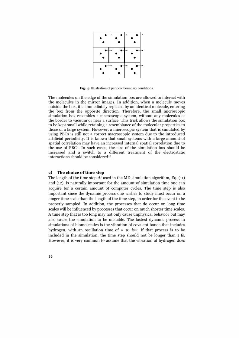
Fig. 4. Illustration of periodic boundary conditions.

The molecules on the edge of the simulation box are allowed to interact with the molecules in the mirror images. In addition, when a molecule moves outside the box, it is immediately replaced by an identical molecule, entering the box from the opposite direction. Therefore, the small microscopic simulation box resembles a macroscopic system, without any molecules at the border to vacuum or near a surface. This trick allows the simulation box to be kept small while retaining a resemblance of the molecular properties to those of a large system. However, a microscopic system that is simulated by using PBCs is still not a correct macroscopic system due to the introduced artificial periodicity. It is known that small systems with a large amount of spatial correlation may have an increased internal spatial correlation due to the use of PBCs. In such cases, the size of the simulation box should be increased and a switch to a different treatment of the electrostatic interactions should be considered26.

c) The choice of time step

The length of the time step ∆t used in the MD simulation algorithm, Eq. (11)

and (12), is naturally important for the amount of simulation time one can

acquire for a certain amount of computer cycles. The time step is also

important since the dynamic process one wishes to study must occur on a

longer time scale than the length of the time step, in order for the event to be

properly sampled. In addition, the processes that do occur on long time

scales will be influenced by processes that occur on much shorter time scales.

A time step that is too long may not only cause unphysical behavior but may

also cause the simulation to be unstable. The fastest dynamic process in

simulations of biomolecules is the vibration of covalent bonds that includes

hydrogen, with an oscillation time of ≈ 10 fs27. If that process is to be

included in the simulation, the time step should not be longer than 1 fs.

However, it is very common to assume that the vibration of hydrogen does

17

not influence the much larger scale processes under study, such as protein

folding and unfolding. The covalent bonds that include hydrogen in both the

solvent and the protein can therefore be constrained at a fixed distance by

algorithms such as SHAKE28 or LINCS29. The SETTLE algorithm30 can be

used for completely rigid water, i.e. when the bond angle of water is

constrained as well as the bond lengths. Constraining covalent bonds to

hydrogen allows for an increase of the time step to 2 fs. Other tricks to

increase the time step exist. For example, increasing the mass of the

hydrogen atom while at the same time decreasing the mass of the covalently

bonded heavy atom, will decrease the oscillation frequency of that bond or

angle. This allows for a longer time step. The potential functions used in the

force field can also be smoothed in order to decrease the forces and thereby

the dynamics of the system. Naturally, the effect of such changes must be

carefully evaluated27.

d) All-atom force fields versus United-atom force fields

The computational demand of an MD simulation algorithm scales with the

number of atoms. All-atom force fields treat every individual atom in the

system explicitly. United-atom force fields do not treat every individual atom

but instead merge a few atoms together into only one interaction site. The

properties of the new united-atom can be derived from the properties of the

individual atoms. It is common in the treatment of aliphatic residues to

merge hydrogen atoms with the carbon atoms that they are covalently

bonded to. This can significantly reduce the number of interactions sites for

proteins and lipid membranes and the simulations are therefore less

computationally demanding. Hydrogen atoms on polar residues are often

explicitly treated in order to facilitate the description of hydrogen bonding14.

18

2.2. Nuclear Magnetic Resonance Spectroscopy

Elementary particles have a quantum mechanical property called spin. The

spin of a particle corresponds to a certain degree of angular momentum of

that particle. However, spin is an intrinsic property of the particle, lacking a

classical analogue. Since elementary particles have spin, composite particles,

such as atomic nuclei, also have a certain spin, see Table 1.

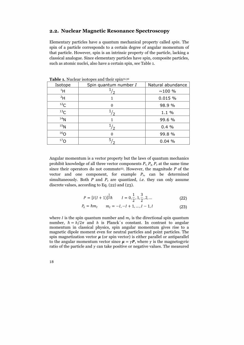
Table 1. Nuclear isotopes and their spin31,32

Isotope Spin quantum number I Natural abundance 1H 1 2~ ~100 % 2H 1 0.015 % 12C 0 98.9 % 13C 1 2~ 1.1 % 14N 1 99.6 % 15N 1 2~ 0.4 % 16O 0 99.8 % 17O 5 2~ 0.04 %

Angular momentum is a vector property but the laws of quantum mechanics

prohibit knowledge of all three vector components Px, Py, Pz at the same time

since their operators do not commute33. However, the magnitude P of the

vector and one component, for example Pz, can be determined

simultaneously. Both P and Pz are quantized, i.e. they can only assume

discrete values, according to Eq. (22) and (23).

� � ��2� 4 13�-#� � � 0, 12 , 1, 32 , 2, … 1/2

(22)

�� � �!� !� � ��, �� 4 1, … , � � 1, �

(23)

where � is the spin quantum number and !� is the directional spin quantum number, � � �/2] and � is Planck´s constant. In contrast to angular momentum in classical physics, spin angular momentum gives rise to a magnetic dipole moment even for neutral particles and point particles. The spin magnetization vector � (or spin vector) is either parallel or antiparallel to the angular momentum vector since � � ��, where � is the magnetogyric ratio of the particle and � can take positive or negative values. The measured

19

magnetization of a particle with spin quantum number � has 2� 4 1 different values along a defined external axis, according to Eq. (23). These spin states are degenerate when no external magnetic field is applied. When an external magnetic field is applied, the spin states will have different energy and the spin vector will align with the external field in order to minimize its energy. This is called the Zeeman effect. The energy of a magnetic moment � in an external magnetic field � is

d � �� · � � ��� · �

(24)

Let us define the direction of the external field as the z-direction. The energy of a spin state is then

d � ����� � ���!��

(25)

Since P > PZ according to Eq. (22) and (23), the spin vector cannot be parallel to the external field. Instead, the spin vector tilts relative to the

external field with an angle of D � cos�- ���� �. The magnitude of Px and Py are

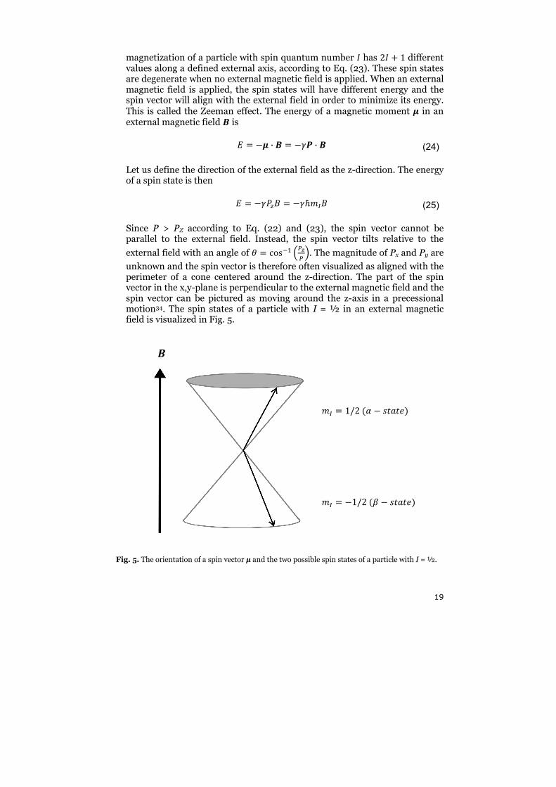
unknown and the spin vector is therefore often visualized as aligned with the perimeter of a cone centered around the z-direction. The part of the spin vector in the x,y-plane is perpendicular to the external magnetic field and the spin vector can be pictured as moving around the z-axis in a precessional motion34. The spin states of a particle with I = ½ in an external magnetic field is visualized in Fig. 5.

!� � �1/2 2� � �&�&�3

!� � 1/2 2� � �&�&�3

�

Fig. 5. The orientation of a spin vector � and the two possible spin states of a particle with I = ½.

20

In the field of Nuclear Magnetic Resonance (NMR) spectroscopy, one

induces transitions among the spin states of atomic nuclei placed in an

external magnetic field. The frequency condition is:

h�A � Δd � |���∆!�|

(26)

where the frequency �A of the electromagnetic radiation corresponds to radio

wave frequency. The angular frequency �A � �A2] is known as the Larmor

frequency and has the same value as the rate of precession of the spin vector

around the z-axis. The sample is subjected to a short pulse of

electromagnetic radiation in order to induce excitation of the nuclei under

study. A pulse of high power and with a long duration will cause many nuclei

to be excited. The pulse will also cause the spin vectors of the individual

nuclei to become phase coherent in the x,y-plane. Pulses with certain

strengths and durations are named after the angle that they flip the total

magnetic moment vector of the sample � � ∑ �%% . A 90° pulse is therefore a

pulse that flips the �-vector from the z-axis down to the x,y-plane. The

motion of the magnetic moment vector in the x,y-plane induces a current in

the nearby coils. The strength and the frequency of this current are recorded

and a Fourier transform of the data yields a frequency spectra. A 180° pulse

has ~twice the duration of a 90° pulse and inverts the magnetic moment in

the z-direction.

Nuclear spin relaxation

The excitation of the nuclear spins by the electromagnetic pulse causes the

sample to deviate from the Boltzmann distribution of the given temperature.

Interactions between the nuclei under study and their surroundings cause

relaxation of the spins and the sample thereby returns to thermal

equilibrium. Even though the relaxation of the spins causes the observed

signal to decay, the relaxation process can also be a useful source of

information of the dynamics in the sample34. Bloch has described the

relaxation process on a macroscopic level35. The relaxation is assumed to be

exponential but the relaxation in the z-direction is allowed to occur with a

different rate than in the x,y-plane. The relaxation in the z-direction is given

by:

"∆��2&3"& � ��-∆��2&3

(27)

∆��2&3 � ��2&3 � �>�

(28)

21

where �>� is the equilibrium magnetization in the z-direction. Solving the

differential equation, Eq. (27), yields:

∆��2&3 � ∆��203exp 2��-&3 (29)

For a frame of reference that rotates with the magnetization in the x,y-plane,

the corresponding equations for the x- and y-components are given by:

"��,�2&3"& � ��#��,�

(30)

and

��,�2&3 � ��,�203 exp 2��#&3 (31)

The relaxation rates R1 and R2 have corresponding relaxation times by the relations R1=1/T1 and R2=1/T2. The relaxation in the z-direction is called longitudinal relaxation or spin-lattice relaxation and T1 is therefore the spin-lattice relaxation time. The relaxation in the z-direction is responsible for restoring the Boltzmann populations of the spin states. The relaxation in the x,y-plane is called transverse relaxation or spin-spin relaxation and T2 is the corresponding relaxation time. The spin-spin relaxation is responsible for the loss of signal due to dephasing of the spin vectors in the x,y-plane.

T1 can be measured by the inversion recovery method utilizing the pulse

sequence

�180° � w � 90° � 2t�&� &(¡L3 � =� (32)

where the time delay Td is added in order to let the system relax back to the

Boltzmann populations between each acquisition. T2 can be measured by the

spin-echo pulse sequence

¢90°� � w/2 � 180°� � w/2 � 2t�&� &(¡L3 � =£ (33)

T2 is inversely related to the spectral peak-width, i.e. short T2 give broad

peaks. However, the external magnetic field is often slightly inhomogeneous,

which leads to a varying field strength over the sample volume. This adds to

the transverse relaxation and T2 measured from the peak widths is therefore

often shorter than T2 from a spin-echo measurement31,34.

While the Bloch equations are macroscopic, a microscopic spin relaxation theory is provided by the works of Bloch-Wangsness-Redfield36,37,38 (BWR). Even though it is possible to fully treat spin relaxation by quantum

22

mechanics, the simpler semi-classical approach of the BWR theory has proven to be very useful. The spin (spins) under study is then treated quantum mechanically but the surroundings are treated classically. The weak coupling between the surroundings and the spin system is the source of the observed spin relaxation. A number of different relaxation mechanisms

for nuclear spins exist. Relaxation mechanisms for nuclei with � � -# are

based upon fluctuating magnetic fields that originates from the thermal motion of the molecules. However, nuclei with spin quantum number � ¤ 1, can also relax via the quadrupolar mechanism, which usually dominates over the other mechanisms. Nuclei with � ¤ 1 have an electric quadrupole moment, in addition to the magnetic dipole moment. The electric quadrupole moment can be visualized as two electric dipole vectors that are positioned back-to-back. The magnetic dipole moment induced by the spin of the nucleus is parallel or at a right angle to the electric quadrupole34. The electric quadrupole of the nucleus interacts with the electric field gradient

components of the surroundings, ¥¦§¥%¥W where (, ¨ � ©, ª, « and o is the

electrostatic potential at the position of the nucleus. The electric field gradient originates primarily from the molecule containing the nuclei under study. The electric quadrupole moment will therefore couple with the molecular frame while the spin vector couples with the external magnetic field. Thermal tumbling of the molecule may therefore induce spin relaxation via the quadrupolar mechanism.

The Hamiltonian of the spin system can be written as: ¬ � ¬A 4 ¬-2&3, where ¬A is the time-independent Zeeman interaction. ¬-2&3 is the stochastic time-dependent perturbation on the spin system that originates from the surroundings. ¬-2&3 will differ depending upon the relaxation mechanism under study. If we neglect other interactions than the quadrupole interaction, ¬-2&3 contains the electric field gradient components, spin operators and physical constants, such as the quadrupole moment of the nucleus. The electric field gradient will fluctuate with the molecular tumbling and this movement is responsible for the time-dependence of ¬-2&3. A correlation function ­2w3 can be defined as

­2w3 �® ¬-2&3¬-2& 4 w3 ¯ (34)

The correlation function will decay with increasing w with a characteristic

time constant w}, called the correlation time. The correlation time is defined

as

w} � v ­2w3­203 "wxA

(35)

23

The correlation time and the shape of ­2w3 are indicative of the rate of

fluctuations of the interaction ¬- between the spin system and the

surroundings. The frequency components of these fluctuations can be

extracted by performing a Fourier transform of ­2w3. We define the spectral

density °2�3 as

°2�3 � v ­2w3��%±²"wx�x

(36)

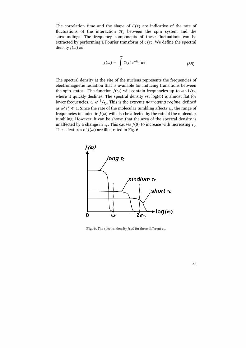
The spectral density at the site of the nucleus represents the frequencies of

electromagnetic radiation that is available for inducing transitions between

the spin states. The function °2�3 will contain frequencies up to �~1/w},

where it quickly declines. The spectral density vs. log(ω) is almost flat for

lower frequencies, � ´ 1 w}~ . This is the extreme narrowing regime, defined

as �#w}# ´ 1. Since the rate of the molecular tumbling affects w}, the range of

frequencies included in °2�3 will also be affected by the rate of the molecular

tumbling. However, it can be shown that the area of the spectral density is

unaffected by a change in w}. This causes °203 to increase with increasing w}.

These features of °2�3 are illustrated in Fig. 6.

Fig. 6. The spectral density °2�3 for three different w}.

24

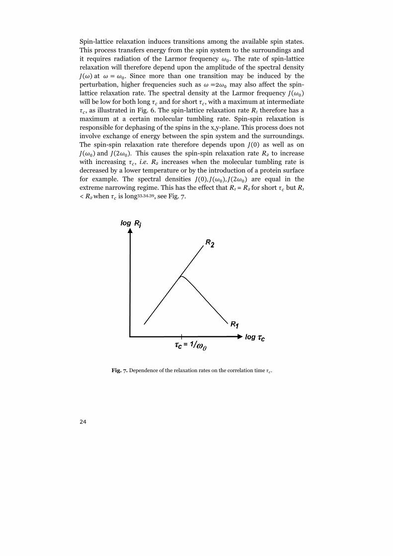
Spin-lattice relaxation induces transitions among the available spin states.

This process transfers energy from the spin system to the surroundings and

it requires radiation of the Larmor frequency �A. The rate of spin-lattice

relaxation will therefore depend upon the amplitude of the spectral density °2�3 at � � �A. Since more than one transition may be induced by the

perturbation, higher frequencies such as � �2�A may also affect the spin-

lattice relaxation rate. The spectral density at the Larmor frequency °2�A3

will be low for both long w} and for short w}, with a maximum at intermediate w}, as illustrated in Fig. 6. The spin-lattice relaxation rate R1 therefore has a

maximum at a certain molecular tumbling rate. Spin-spin relaxation is

responsible for dephasing of the spins in the x,y-plane. This process does not

involve exchange of energy between the spin system and the surroundings.

The spin-spin relaxation rate therefore depends upon °203 as well as on °2�A3 and °22�A3. This causes the spin-spin relaxation rate R2 to increase

with increasing w}, i.e. R2 increases when the molecular tumbling rate is

decreased by a lower temperature or by the introduction of a protein surface

for example. The spectral densities °203, °2�A3, °22�A3 are equal in the

extreme narrowing regime. This has the effect that R1 = R2 for short w} but R1

< R2 when w} is long33,34,39, see Fig. 7.

Fig. 7. Dependence of the relaxation rates on the correlation time w}.

25

The link between NMR spectroscopy and MD simulations

MD simulations are based upon classical physics and do not include

quantum mechanical properties of atoms such as spin. One might therefore

incorrectly assume that MD simulations cannot aid in the analysis of NMR

experiments. In fact, there can be a transfer of information from NMR to MD

as well as in the opposite direction. The link that joins the two methods is the

dynamics of the studied system. Nuclear spin relaxation is induced due to

the fluctuations of electromagnetic fields when the molecules diffuse, as seen

in the correlation function ­2w3 of Eq. (34) and the spectral density of Eq.

(36).

The relaxation rates R1 and R2 measured by NMR can be interpreted in terms

of molecular motion by MD simulations of the same molecular system. MD

simulations can be used to calculate motional correlation functions for

individual molecules, for example at different locations in the system, such

as solvent in the bulk phase versus solvent near a surface. This microscopic

information can be used to disentangle the experimentally obtained spin

relaxation rates that are ensemble averages of the whole macroscopic

system. NMR can therefore contribute with the accuracy of macroscopic

experiments and the longer timescales that are possible to study, while MD

simulations supply information on a molecular level.

3. The Research Field of Chemical Denaturation

The long term aim of research in the field of chemical denaturation is to

explain the molecular mechanism behind the denaturant-induced decrease

in the thermodynamic stability of proteins. However, connecting detailed

molecular properties with thermodynamic stabilities is difficult. The

complexity of such a large scale process as protein unfolding is high. There is

also a very large difference in the time scale of the molecular events in the

solvent that induces the unfolding and the unfolding process itself. The

logical path between molecular properties and free energies is too long to be

covered in one step. One should therefore first explain the affect of urea on

free energies in terms of other thermodynamic properties such as enthalpies

and entropies that are more closely related to the established experimental

facts. When such a connection has been found and understood, the next step

is to link these results to molecular properties and to understand the

mechanism of urea in greater detail.

26

3.1. The Thermodynamics of Protein – Urea Systems

Denaturation curves

The effect of urea is general, i.e. all proteins are destabilized by the addition

of urea, but in order to invert the populations of folded versus unfolded

protein, very high concentrations of urea, up to 9 M, are usually needed. This

strongly indicates that the interaction between urea and the proteins are

weak. Unfortunately, a weak interaction is more difficult to study than a

strong interaction. The concentration of urea that is needed to denature a

protein, depends on the type of protein. Lysozyme from hen egg white

cannot in a practical way be unfolded by urea at physiological pH and room

temperature since very high urea concentrations are needed40. Anyway, the

stability of lysozyme is lower in a urea solvent than in water even if complete

unfolding is not reached. Studies have also shown that some proteins retain

residual structure when they have been unfolded in urea41,42,107.

The amount of urea that must be added to a protein – water solution in order

to unfold a certain protein depends on the stability of the protein in water,

∆�����,¶#·, as well as on the degree of dependence of ∆����� on the urea

concentration. The concentrations of the folded and the unfolded protein at a

specific urea concentration can be measured by for example circular

dichroism or fluorescence spectroscopy43,44. The stability of the protein at

that specific urea concentration can then be calculated by using Eq. (2) and

(3). If the protein contains one of the fluorescent amino acids tryptophan

(Trp), tyrosine (Tyr) or phenylalanine (Phe), these can be used as internal

probes for fluorescent spectroscopic measurements. Otherwise, external

fluorescent probes must be attached to the protein. Tryptophan is the most

popular of the internal probes since the quantum yield is high, which causes

the fluorescence intensity to be high. In addition, the fluorescence intensity

of tryptophan is very sensitive to the molecular environment, which makes it

a good probe of structural changes in the protein. Tryptophan is hydrophobic

and is therefore often located in the core of the protein. The amount of

solvent contact of the residue is likely small in the folded state but will

increase during unfolding. When the molecular environment of an amino

acid changes, the fluorescence intensity of that amino acid will change as

well. From the graph of fluorescence intensity as a function of the urea

concentration, the concentrations of the folded and the unfolded protein can

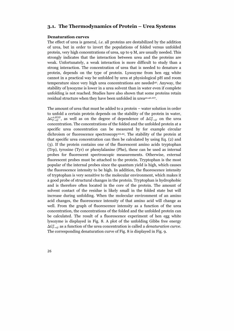
be calculated. The result of a fluorescence experiment of hen egg white

lysozyme is displayed in Fig. 8. A plot of the unfolding Gibbs free energy

∆����� as a function of the urea concentration is called a denaturation curve.

The corresponding denaturation curve of Fig. 8 is displayed in Fig. 9.

27

Urea concentration [M]

0 2 4 6 8 10

Fluorescence intensity

0

100

200

300

Folded Mix Unfolded

Fig. 8. Denaturation curve of hen egg white lysozyme at pH 3 as obtained by fluorescence after

excitation at 280 nm and emission at 360 nm.

Col 1 vs Col 2

Col 3 vs Col 6

0 2 4 6 8 10

∆∆ ∆∆Go

F-U [kJ/mol]

-20

-10

0

10

20

30

40

Urea concentration [M]

Folded Mix Unfolded

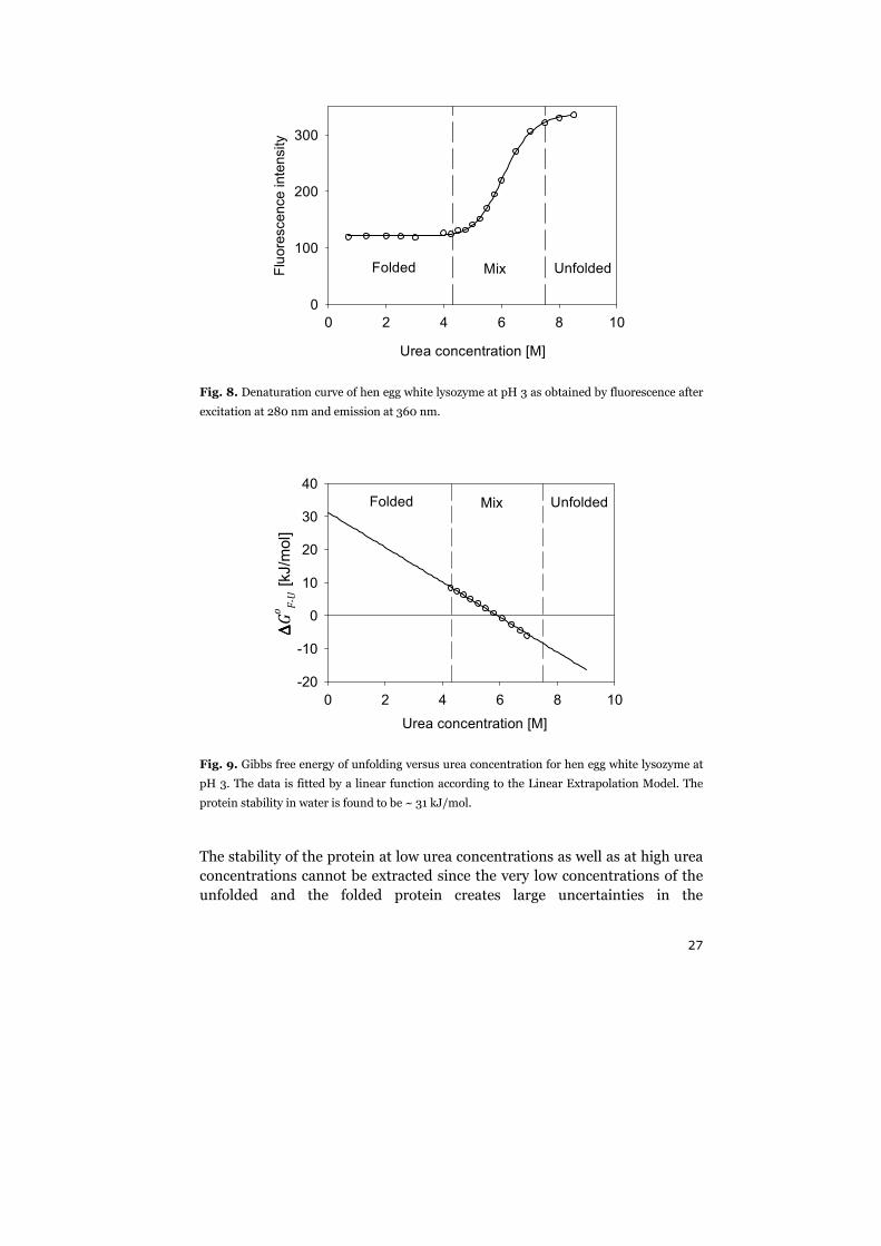
Fig. 9. Gibbs free energy of unfolding versus urea concentration for hen egg white lysozyme at

pH 3. The data is fitted by a linear function according to the Linear Extrapolation Model. The

protein stability in water is found to be ~ 31 kJ/mol.

The stability of the protein at low urea concentrations as well as at high urea

concentrations cannot be extracted since the very low concentrations of the

unfolded and the folded protein creates large uncertainties in the

28

equilibrium constants at those urea concentrations. The protein stability in

pure water, ∆�����,¶#·, is an interesting property to measure in protein

research. Unfortunately, this property cannot be extracted by other means

than an extrapolation of the denaturation curve to zero urea concentration.

Several theoretical models have been developed in order to make the

extrapolation as correct as possible. These models are based upon varying

amounts of empirical evidence and thermodynamic arguments. The simplest

but also the most widely used model is the Linear Extrapolation Model45. It

assumes a linear relationship between the free energy of unfolding and the

denaturant concentration. The stability of the protein in water can then

simply be found by linear regression of the experimental data and

extrapolating to zero denaturant concentration. This model therefore does

not require any additional data other than the denaturation curve, but does

not give any insight into the denaturation mechanism either. The slope of the

fitted line is the so-called m-value, ! � � ¥∆¸¹�º»¥��P>E�, and represents the

efficiency of the denaturant in destabilizing that particular protein. The m-

value has been shown to be proportional to the increase in the solvent

accessible surface area (SASA) of the unfolded protein as compared to the

folded protein46. Despite the simplicity of this model, it yields similar values

of ∆�����,¶#· as those obtained from thermal denaturation45, at least for urea

denaturation. However, some denaturation curves are not linear for low urea

concentrations47 and are better fitted with a quadratic model for instance48.

The Transfer Model (Tanford´s Model)73 is based uon experimental data of

the free energies of transfer of amino acids from water to a denaturant

solution. The amino acid composition of the protein as well as estimations of

the SASA of the amino acids in the folded protein versus in the unfolded

protein, are needed in order to extract the free energy of unfolding in water.

The Denaturant Binding Model49 links the effectiveness of a denaturant to

preferential binding of this denaturant to the protein surface in the folded

and the unfolded state.

Among these three models, linear extrapolation always gives the smallest

estimated values of ∆�����,¶#·. The difference is small for urea but larger for

guanidinium chloride. Since guanidinium chloride is a salt, the deviation

from simple thermodynamics relationships may be due to electrostatic

effects, such as screening of the protein charges50,51. Urea is considered to be

more reliable for denaturation studies than guanidinium chloride. Other

models than the three mentioned here have been proposed as well52,53,54.

It is possible to extract Δ�����,¶#· without using denaturants. Thermal denaturation of proteins by Differential Scanning Calorimetry (DSC) is

29

commonly used to gain knowledge about the thermodynamics of unfolding of the protein under study55. By sweeping the temperature of the sample compartment containing the protein solution, the melting temperature Tm is found at which the protein unfolds. The enthalpy change ∆Hm of the unfolding process at Tm can be extracted, as well as the heat capacity change,

∆Cp. These data can then be used to calculate Δ�����,¶#· at an arbitrary temperature by making use of the Gibbs-Helmholtz equation:

Δ�����,¶#·23 � ¼½Q� 81 � Q9 4 ¼­R� � Q � ¾L2/Q3�

(37)

As for the analysis of denaturation curves, the extrapolation introduces

uncertainties in the value of Δ�����,¶#·. However, comparisons of protein

stabilities obtained by DSC and chemical denaturation show that they are in

agreement, within the experimental uncertainties of the two methods45,56.

Experimental studies of the thermodynamics of urea

In order to understand the destabilizing effect of urea on the folded protein,

studies of the thermodynamics of protein – urea solution systems are

essential. However, first it is necessary to understand why proteins fold in

water. In a simple view of folding, two terms favor the folded state and one

term favors the unfolded state. The unfolded protein has more solvent

contact then the folded protein. Protein – water interactions are therefore

replaced by protein – protein and water – water interactions during folding.

These changes will in general decrease the enthalpy of the system and this

term therefore favors the folded state. The other term that favors the folded

state is the hydrophobic effect. The non-bonded interactions between water

and hydrophobic side chains are weak, which increases the enthalpy of the

water. In addition, the weak interactions also lead to a decrease in the

entropy of water since the conformational flexibility of the water around

hydrophobic solutes becomes restricted. Therefore, there are both enthalpic

and entropic driving forces that lead to the clustering of hydrophobic side

chains in folded proteins. The temperature dependence reveals that the

hydrophobic effect is dominated by entropic driving forces at room

temperature but that enthalpic driving forces make significant contributions

at higher temperatures57. The term connected with the change of interactions

during folding and the hydrophobic effect is thought to contribute equally to

the stability of proteins.

The term that favors the unfolded state is the conformational entropy of the

protein. The entropy of the protein decreases during folding, since the

conformational flexibility is greatly reduced in the folded state as compared

30

to the unfolded state. In total, the terms that stabilize and destabilize the

folded protein are both large and almost equal. The net protein stability is

therefore often very small58.

We now return to the discussion of thermodynamics of proteins - urea

solutions. However, due to the complexity of such systems, proteins have in

some studies been replaced by model compounds or individual amino acids.

When Nozaki and Tanford measured the free energy of transfer of eleven

amino acids from water to a urea solution in the sixties, they found that nine

of the amino acids had a negative transfer free energy59. Only the smallest

amino acids glycine and alanine had positive transfer free energies. This

result indicates that both polar and hydrophobic amino acids contribute in

the unfolding and also that the size of the solute molecule might be

important for the affect of urea. Due to the importance of the hydrophobic

effect to the stability of proteins, a natural subject of investigation is the

interaction of urea with hydrophobic solutes. Wetlaufer et al.60 measured

transfer free energies of hydrocarbons and discovered that relatively large

hydrocarbons, such as propane and butane, had negative transfer free

energies from water to urea but very small hydrocarbons, such as methane

and ethane, had positive free energies. This result shows that the

hydrophobic effect may be decreased in urea but the relative importance is

not unveiled. Several MD simulation studies61,62,63,88 have also found that the

interaction between a hydrophobic solute and a urea solvent depends on the

size of the solute. A theoretical treatment of this effect by Graziano could

explain both the dependence on the size of the solute64 and the temperature

dependence of the transfer free energy65 in the data of Wetlaufer et al60. It

was found that cavity formation entropy has a larger negative value in a urea

solution than in water. This effect dominates for small hydrophobic solute

molecules. However, the vdw interaction between the solute and the solvent

is more attractive in the urea solution than in water and this effect dominates

for large hydrophobic solutes. This means that large hydrophobic solutes can

be favorably solvated in a urea solvent due to the enthalpic driving force of

solute – solvent vdw interactions. The favorable vdw interactions with a urea

solution were explained by the high packing density of urea solutions, the

high polarizability and the large dipole moment of the urea molecule64. The

free energy of cavity formation has been confirmed to increase with urea

concentration in a similar theoretical analysis of the transfer experiments66.

The transfer free energy study performed by Robinson and Jencks67

concerned a model compound that resembles a peptide backbone, rather

than hydrophobic side chains. The transfer free energy from water to a urea

solution was negative also for this polar compound. However, it should be

noted that the negative free energy is realized in different ways for two types

31

of compounds. Both the enthalpy and the entropy of transfer of large

hydrocarbons from water to urea are positive, but the corresponding

enthalpy and entropy of transfer of the polar backbone compound are

negative60,67. This has been confirmed in other studies68,69. Interestingly, the

studies of Graziano64,65 shows that the transfer of hydrocarbons from water

to a urea solution or to a guanidinium chloride solution includes a large

amount of hydrogen bond restructuring between solvent molecules. This

effect is connected with large positive enthalpic and entropic terms that are

included in the experimentally measured transfer thermodynamics.

However, it can be shown that the entropic term �∆¿° and the enthalpic

term of hydrogen bond restructuring exactly cancel each other for solutions

where the solute – solvent interactions are weak as compared to the solvent

– solvent interactions. This applies to a urea solution with a hydrocarbon

solute and the effect of hydrogen bond restructuring can therefore be

removed from the calculation of the free energy. It is then found that the

transfer of hydrocarbons from water to a urea solution is characterized by a

negative enthalpy term and a negative entropy term. Transfer of both

hydrocarbons and the backbone compound are therefore driven by an

enthalpic driving force. The main results of Graziano are supported by an

MD simulation study of neo-pentane solvation70. The results are also in

agreement with a calorimetric study of the interaction between urea and

three globular proteins71. The addition of urea from 0 M to 2 M was seen to

promote protein unfolding by decreasing the enthalpy of unfolding. The

entropy of unfolding was also decreased but the effect on the enthalpy was

larger and urea therefore decreased the Gibbs free energy of unfolding. The

results of another calorimetric study of five globular proteins were similar72.

The enthalpies of interaction between urea and the proteins were exothermic

for all proteins and the unfolding was exothermic in urea, in contrast to the

endothermic unfolding in water.

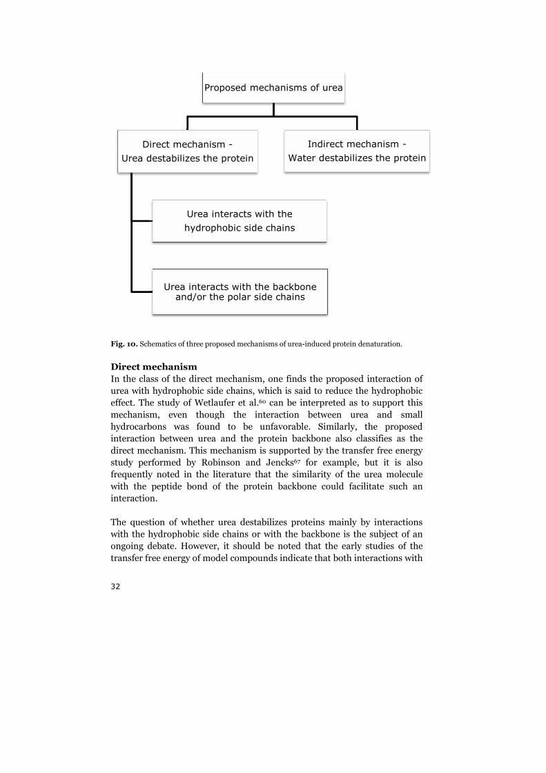
3.2. Proposed Mechanisms of Urea-Induced Denaturation

A number of mechanisms of urea-induced denaturation have been proposed.

These different mechanisms have been categorized according to whether

urea interacts and destabilizes proteins by itself, the so called direct

mechanism, or if urea instead acts on water and thereby change the

properties of the water into a solvent that destabilizes proteins. This is called

the indirect mechanism. From these two classes, three proposed

mechanisms have gained the most attention with a number of papers in

support of, or against, each mechanism.

32

Fig. 10. Schematics of three proposed mechanism

Direct mechanism

In the class of the direct mechanism, one finds the proposed interaction of

urea with hydrophobic side chains, which is said to reduce the hydrophobic

effect. The study of Wetlaufer et al

mechanism, even though the interaction between urea and small

hydrocarbons was found to be unfavorable

interaction between urea and the protein

direct mechanism. This mechanism is supported by

study performed by Robinson and Jencks

frequently noted in the literature that the similarity of the urea molecule

with the peptide bond of the protein backbone

interaction.

The question of whether urea destabilizes proteins mainly by interactions

with the hydrophobic side chains or with the backbone

ongoing debate. However, it should be noted that the early studies of the

transfer free energy of model compounds indicate that both interactions with

Proposed mechanisms of urea

Direct mechanism -

Urea destabilizes the protein

Urea interacts with the

hydrophobic side chains

Urea interacts with the backbone and/or the polar side chains

mechanisms of urea-induced protein denaturation.

In the class of the direct mechanism, one finds the proposed interaction of

, which is said to reduce the hydrophobic

The study of Wetlaufer et al.60 can be interpreted as to support this

, even though the interaction between urea and small

hydrocarbons was found to be unfavorable. Similarly, the proposed

interaction between urea and the protein backbone also classifies as the

This mechanism is supported by the transfer free energy

study performed by Robinson and Jencks67 for example, but it is also

that the similarity of the urea molecule

of the protein backbone could facilitate such an

The question of whether urea destabilizes proteins mainly by interactions

with the hydrophobic side chains or with the backbone is the subject of an

However, it should be noted that the early studies of the

transfer free energy of model compounds indicate that both interactions with

Proposed mechanisms of urea

Urea interacts with the

hydrophobic side chains

Urea interacts with the backbone and/or the polar side chains

Indirect mechanism -

Water destabilizes the protein

33

the hydrophobic side chains and the backbone should contribute to the

destabilizing effect of urea. The conclusions of Tanford73 and of Wetlaufer et

al.60 were that the interactions between urea and the hydrophobic side

chains and with the backbone make equal contributions for the effect of urea

on proteins.

Indirect mechanism

Some controversy exists about the structure of the binary urea – water

solution. The papers of Schellman74, Kresheck - Scheraga75 and Stokes76

constitute the SKSS model of the urea solution structure. They proposed that

the water structure is unchanged by urea but that urea itself forms dimers

and oligomers due to hydrogen bonds between the -NH and –CO groups,

similar to the hydrogen bonded secondary structures found in proteins.

Papers in support of the SKSS model exist, see for example Ref. 77. However,

the rotational correlation time of urea in water solution has been obtained by

NMR and it indicates that the majority of urea exists in the monomer form in

water solution78. A study of the urea solution structure by using Raman

spectroscopy did not find any evidence for urea dimers79.

Another model of the structure of urea – water solutions, the Frank-Franks

(FF) model80, forms the basis of the indirect mechanism of urea-induced

protein denaturation. According to this model, urea decreases the structure

of water, i.e. urea acts as a chaotrope. The ordering of water close to

hydrophobic surfaces is therefore possibly reduced by urea, thereby making

water better at accommodating hydrophobic solutes. The ideas of this

mechanism originate from a theoretical analysis80 of the transfer study of

hydrocarbons performed by Wetlaufer et al60. In the employed theoretical

model, water is treated as composed of two different phases, one bulky and

highly hydrogen bonded structured phase and one dense phase with less

structure. Urea is pictured as being soluble only in the dense, unstructured

water phase, thus lowering the chemical potential of that phase. In order to

maintain equilibrium with the structured water phase, the equilibrium is

shifted towards the water phase with less structure, i.e. urea is a water

structure breaker. Hydrocarbons are said to increase the structure of water

but this effect can be counteracted by the structure breaking effect of urea

and there is therefore a gain in entropy associated with the transfer of

hydrocarbons from water to a urea solution, as experimentally observed60.

Studies aiming at investigating the proposed water structure breaking effect of urea have been conducted. As for the SKSS model, some studies show results in accordance with the FF model and the indirect mechanism of chemical denaturation, see for example Ref. 78,81,82. In contrast, some studies find that urea increases the water structure85,83 and propose that this

34

can also explain the denaturation of proteins. Even though this discussion has not been settled, it seems that the present view is that urea does not alter the water structure to any high degree. This conclusion is supported by a number of studies3,61,77,88,105. If this is true, urea does not denature proteins by the indirect mechanism.

3.3. MD Simulation Studies of Chemical Denaturation The MD simulation technique has been utilized in studies of the structural

properties61,83,84, the dynamics85,86 and the solubility properties61,62,84,87,88 of

the urea / water mixture. MD simulations have also been used in studying

the effect of urea on peptides and model compounds89,90,91,92,93,94,95 as well as

on proteins96,97,98,99,100,101,102,103,104,105,106,107,108. Some studies were published as

early as the 1980s but the results from those studies are vague due to the

very short simulations (ps - ns) as compared to the timescale of protein

unfolding (µs – ms). Simulations long enough to show the majority of an

unfolding trajectory have only been possible in the last few years. At present,

simulations of the complete unfolding of small to medium sized proteins are

possible but elevated temperatures are often needed in order to accelerate

the unfolding.

A clear result from the MD simulation studies is that urea has a higher

concentration close to the protein surface than in the bulk phase, see for

example Ref. 89, 90, 94, 95. In the simulations of Stumpe and Grubmüller,

the concentration of urea was found to be especially high at the hydrophobic

amino acids and water preferentially solvated the charged amino acids. They

argue that this effect is due to electrostatic interactions, rather than

Lennard-Jones interactions or entropic factors. Unfortunately, the cutoff in

the analysis of the force field energies was short, which raises doubts about

the results. Still, in additional simulations107 they found that a urea model

with downscaled charges denatures proteins much faster than the urea

model with the original charges. Urea with upscaled charges even seemed to

stabilize the protein. It was therefore suggested that “apolar urea-protein

interactions, and not polar interactions, are the dominant driving force for

denaturation”. The interaction between urea and the hydrophobic parts of

the protein was also found to impede the hydrophobic collapse of partially

unfolded proteins106.

In contrast, the research group of Thirumalai has published a number of

papers90,91,95 where they argue that urea denatures proteins primarily by the

direct mechanism but via electrostatic interactions with the protein

backbone or polar side chains. However, they incorrectly assume that the

35

stabilization of methane in a urea solution as compared to in water (as seen

in their calculations of the potential of mean force PMF) apply to larger

hydrophobic solutes as well. In addition, the negligible effect of urea on the

PMF of an ionic pair is not significantly discussed91. They note that urea

accumulates near the protein surface, as seen in radial distribution functions

(RDFs). Significant hydrogen bonding can also be seen between the peptide

and the urea molecules and this is interpreted as a main cause of the effect of

urea on proteins90. However, the cause-and-effect relation between the

accumulation of urea near the peptide and the number of hydrogen bonds is

not investigated further. The relation between the hydrogen bonding and the

protein destabilization is also assumed without more analysis. In Ref. 95, the

unfolding equilibrium of a hydrocarbon chain is studied in water and 6 M

urea. Strangely, it was found that the folded structure of the hydrocarbon

was destabilized by introducing charges of different signs at the ends of the

hydrocarbon chain. This result can perhaps be traced to inadequate

sampling due to the limited simulation lengths of 3 - 4 ns.

As mentioned in the section regarding experimental studies of the

thermodynamics of urea, support has been found that the dependence of the

transfer free energy upon the solute size is caused primarily by van der

Waals interactions. This is in agreement with an MD simulation study of ion

solvation in urea solutions88. They conclude that enthalpic interactions

rather than entropic cause the dependence on solute size. Furthermore,

these results gain support from a study105 of MD simulations of Lysozyme in

a urea solution and of MD simulations92 of hydrophobic model compounds.

In these studies, the non-bonded interactions were divided between the

Lennard-Jones and the electrostatic constituents. It was found that the

Lennard-Jones interaction between the protein and urea was more attractive

than between the protein and water. On the other hand, no support could be

found for the indirect mechanism. Both studies conclude that the Lennard-

Jones interaction between protein and urea is likely to be the main cause for

the protein denaturation observed in their MD simulations.

The relative importance of electrostatic and Lennard-Jones interactions for

chemical denaturation in MD simulations was investigated in a recent

paper108. Both electrostatic and Lennard-Jones interactions were reported to

be more favorable between proteins and a urea solvent as compared to

between proteins and water. Unfortunately, the short denaturation processes

(< 30 ns at 325 K) and the very large difference in the potential energy of

urea between the bulk phase and the protein solvation shell (a factor of 2)

raises doubts about the setup and the analysis of the simulations.

36

When reviewing the MD simulation studies on chemical denaturation, it

becomes apparent that it has been unclear what observable to calculate from

the simulation data in order to understand the unfolding. Many studies

describe the unfolding trajectory visually and in terms of structural

parameters of the protein. However, only one or a few replicate simulations

can be performed and analyzed due to the limited computer performance

available. It is then uncertain if the analyzed trajectories are representative

of all possible unfolding pathways. In addition, these systems are not in

equilibrium. If we are to connect the experimentally observed

thermodynamic properties of unfolding with results of simulations, the

simulation systems must be kept in equilibrium and the calculated

properties must be averaged over many replicate simulations.

Several papers89,93,96,98,101 include an analysis of the hydrogen bonding

between solvent molecules and between urea / water and the protein.

Properties such as the life-times and the bond lengths of these hydrogen

bonds are calculated. Also for this type of analysis, it is unclear how to

connect the calculated properties with the destabilization of the protein

without introducing a high degree of assumption.

As was written in the beginning of Chapter 3, the long term goal of the

research concerning chemical denaturation is to explain the molecular

mechanism behind the denaturant-induced decrease in the thermodynamic

stability of proteins. In my opinion, this cannot be done in one step. The

effect of urea on the thermodynamic properties of protein – urea solution

systems must be established first. Experimental techniques such as DSC and

ITC are needed in thermodynamic studies, but they should be accompanied

by MD simulations so that the various enthalpic and entropic terms can be

separated, in order to attain a greater level of detail.

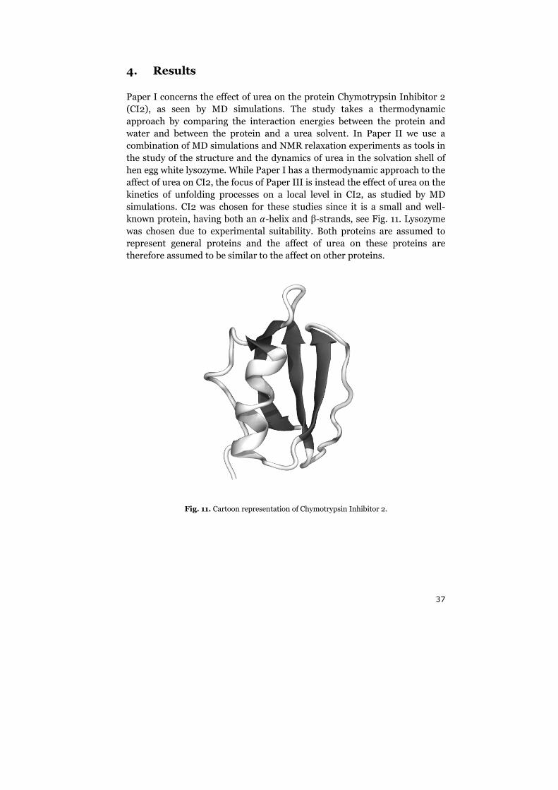
37

4. Results

Paper I concerns the effect of urea on the protein Chymotrypsin Inhibitor 2

(CI2), as seen by MD simulations. The study takes a thermodynamic

approach by comparing the interaction energies between the protein and

water and between the protein and a urea solvent. In Paper II we use a

combination of MD simulations and NMR relaxation experiments as tools in

the study of the structure and the dynamics of urea in the solvation shell of

hen egg white lysozyme. While Paper I has a thermodynamic approach to the

affect of urea on CI2, the focus of Paper III is instead the effect of urea on the

kinetics of unfolding processes on a local level in CI2, as studied by MD

simulations. CI2 was chosen for these studies since it is a small and well-

known protein, having both an �-helix and β-strands, see Fig. 11. Lysozyme

was chosen due to experimental suitability. Both proteins are assumed to

represent general proteins and the affect of urea on these proteins are

therefore assumed to be similar to the affect on other proteins.

Fig. 11. Cartoon representation of Chymotrypsin Inhibitor 2.

38

Paper I

MD simulations of CI2 in water as well as in 10 M urea were performed. The

systems must be in equilibrium in order to extract the effect of urea on

quantities of equilibrium thermodynamics. The folded structure of CI2 in a

10 M urea solution is not an equilibrium system since the protein will

undergo unfolding as a response to the presence of urea. We therefore

restricted the protein to the folded state by employing positional restraint

potentials on the α-carbons. The restraints will counteract the influence of

urea and keep the system in a forced equilibrium state when the protein is

dissolved in 10 M urea. The restraint potentials will necessarily affect the

folded protein by reducing the phase space available to it. In order to be able

to compare the simulations in urea and in water, it was therefore necessary

to employ the same restraints on the protein in water as well. The use of

positional restraints may influence the absolute values of the interaction

energies but the flexible side chains will help to keep this effect small and,

more importantly, the trend in the data is still visible. A positive side effect of

the reduction of the phase space of the folded state is that the sampling is

facilitated.

The protein atoms were classified as belonging to either the backbone, the

hydrophilic side chains or the hydrophobic side chains. MD simulations

where CI2 was solvated by either water or by 10 M urea were performed and

compared with respect to the protein – solvent interaction energies. The

change in the internal energy of this system due to protein unfolding can be

written as a sum of three terms as in Eq. (38).

∆�� � ∆�RP;À>%<� 4 ∆�B;Gy><À� 4 ∆�RP;À>%<�B;Gy><À� (38)

It is likely that urea affects all three of these terms but to a different extent. The third term, ∆�RP;À>%<�B;Gy><À� , was extensively studied in Paper I with a

shorter analysis of ∆�B;Gy><À� . The results showed that an enthalpic driving

force for urea-induced denaturation exists. The interaction energy between

the solvent and the protein decreased by as much as 12 per cent in the 10 M

urea solvent as compared to in water. In the interplay between protein –

protein, solvent – solvent and protein – solvent interactions, the decrease in

the protein – solvent energies will favor an increased protein - solvent

contact by an increase in the protein SASA. All three parts of the protein; the

backbone, the hydrophilic and the hydrophobic side chains, had a more

favorable interaction with the urea solvent than with water. The protein

surface that opens up to solvent during unfolding will have similar properties

as compared to the folded protein, but perhaps with larger fractions of

backbone and hydrophobic surface. The presence of urea is therefore likely to cause ∆�RP;À>%<�B;Gy><À� to decrease. From the viewpoint of protein –

39

solvent interaction energies, all parts of the protein contribute to the

unfolding of the protein. When separating the protein – solvent interaction

energies into its constituents, electrostatic interactions and Lennard – Jones

interactions, it was found that both the relative and the absolute decreases in

the electrostatic energies were small while the decreases in the Lennard –

Jones energies were large. The origin of the decrease in the protein – solvent

energies was therefore the ability of the urea solution to form attractive

Lennard – Jones interactions with all parts of the protein.

When shifting the viewpoint from the protein to the solvent, it was found

that water molecules in the protein solvation shell had higher interaction

energies relative to bulk water but urea molecules had lower interaction

energies relative to bulk urea. This creates an energetic driving force for the

replacement of water by urea at the protein solvation shell. The enrichment

of urea in the solvation shell has been observed87,88,92,93 but can also be

attributed to the gain in entropy of the system when several restricted water

molecules in the solvation shell are replaced by one large urea molecule, as

commonly noted in the literature.

It is likely that the solvation shell energy relative to bulk solvent energy is

changed when urea is added. However, this change was found to be small

relative to the uncertainties in the calculated energy values. The effect of

urea on ∆�B;Gy><À� could therefore not be calculated.

The intramolecular protein energy, ∆�RP;À>%<� , is a function of the protein

structure but it is unaffected by the solvent, except from changes in the permittivity of the solution. The effect of urea on ∆�RP;À>%<� is therefore small

as long as we compare the same folded and unfolded protein states in both

solvents. However, it is likely that urea does affect which structures that are

incorporated into the folded and the unfolded state. It has been suggested

that the unfolded protein states in different urea concentrations may be

structurally different but thermodynamically similar45. Unfortunately, the

unfolded state in water and the folded state in 10 M urea are difficult to

study experimentally and not much are known about these states. It may be that the change in ∆�RP;À>%<� and ∆�RP;À>%<� when urea is added is mostly due

to this effect, but the lack of information prevents us from estimating the

relative importance of the protein intramolecular term in Eq. (38).

40

Paper II In Paper II, we combined MD simulations with NMR spin relaxation measurements in order to investigate structural and dynamic properties of urea in the solvation shell of hen egg white lysozyme. The relaxation rate of the quadrupolar nuclei 14N in the urea molecule was used as a probe to study the dynamics of individual urea molecules at the protein interface. The urea molecules that are dynamically retarded by the contact with the protein surface will experience significantly enhanced relaxation rates. The fraction of the urea solvent that is in contact with a protein is small, since the protein concentration is relatively low due to the limited solubility. However, by utilizing the fact that the molecules in the solvation shell undergo fast chemical exchange with the bulk phase, the enhanced relaxation rates of the urea molecules in the solvation shell can be seen in the relaxation enhancement of the urea molecules in the bulk phase. The spin-lattice and the spin-spin relaxation rates of 14N in urea were obtained at 100 MHz and 400 MHz magnetic field strengths from samples with or without lysozyme and urea concentrations of 3 M or 8.5 M. The results were analyzed by employing a three-site model with fractions F, B and C of urea, with different intrinsic relaxation rates of urea at each site. The F fraction corresponded to urea in the bulk solvent that did not interact with the protein. The B fraction corresponded to urea molecules that reside in the protein solvation shell but with a residence time shorter than 3 ns. The C fraction was the urea molecules that had a residence time in the solvation shell longer than 3 ns.

The results from the NMR relaxation experiments alone cannot be used to

resolve all parameters of the model, since the model is underdetermined.

However, by combining NMR with results from MD simulations of the same

systems, a full parameter set of the model could be found that successfully

describes the spin-lattice relaxation rates and gave a plausible picture of the

dynamics of urea in contact with a protein surface. This approach can

therefore successfully be used in the study of chemical denaturation. It was

found that the dynamics of the urea molecules in the vicinity of the protein

was similar to water in the same region, when the different sizes of the

molecules were taken into account. The urea molecules were dynamically

retarded by the protein surface but not to a higher degree than water

molecules. The results did not support the hypothesis that specific urea

binding sites exists on the protein71,109,110. Urea is instead dynamic and

diffuses around the protein surface. The interaction between urea and the

protein will therefore be averaged with respect to the orientation of urea and

the type of amino acid.

41

The sample that contained lysozyme in the folded structure, solvated in 3 M

urea, showed a clear field dependence and R2 > R1. This was attributed to the

small C fraction of urea molecules. It could be seen from an MD simulation

of the system that, at any point in time, a few (~3) urea molecules reside in

pockets and grooves at the lysozyme surface with a residence time longer

than 3 ns. These urea molecules have a restricted rotational motion with

respect to the protein surface and the rotational averaging is therefore partly

governed by the rotation of the protein - solvent complex. The rotational

correlation time τ is therefore long and the extreme narrowing condition, �#w}# ´ 1 is not fulfilled. The relaxation rates of the sample with unfolded

lysozyme in 8.5 M urea were not field dependent. It is therefore likely that

the pockets and grooves on the lysozyme surface that seems to be needed for

the long residence times, are absent in the unfolded protein structure. The

topology of the protein surface, rather than the primary structure,

determines the presence of urea molecules with long residence time. Once

again we note the absence of specific urea binding sites on protein surfaces.

Paper III In understanding the mechanism of urea-induced denaturation we require not only knowledge about the thermodynamic basis of denaturation but also how the denaturation is realized on a molecular scale. In Paper III we analyzed the affect of urea on local protein processes from a kinetic view point. After all, the molecular action of urea must occur on a local level but this manifests itself in the large effect on the kinetics of the global folding and unfolding processes. However, this mechanism has not been subjected to much research and is not well understood. One may ask what kind of local processes that are affected by urea and how they are affected. It is also not known if urea actively unfolds small protein structures or if urea instead acts by retarding the refolding of such structures.

In an attempt to understand these mechanisms, the dynamics of protein

processes of different scales were analyzed in protein – water and protein –

urea simulations. Very small processes such as the fluctuation amplitudes of

individual backbone atoms were not affected by urea, even though the

tendency for global unfolding is so much higher in the urea solvent.

However, the effect of urea was clearly seen when studying larger scale

processes. An intra-protein electrostatic bond between the side chains of

methionine and lysine could be seen to fluctuate between the open and

closed forms, both in water and in the urea solvent. Both the rate constants

for the opening and the closing processes were decreased by the addition of

urea. In contrast, the rupture frequencies of the hydrogen bonds of the alpha

42

helix and the C- and N-terminal regions were seen to be increased by urea,

similar to the effect of urea on the global unfolding rate.

Based on these results, we proposed that the effect of urea on the unfolding

rate of protein structures depends on whether the process is isolated or if it is

triggered by the unfolding of other nearby structures. For example, the

fluctuation of a side chain with a high degree of solvent contact occurs

almost independently of other simultaneous processes that occur in the

protein. Both the unfolding rate and the refolding rate of such a process

seem to be decreased by urea, as seen in our study and also noted by Stumpe

and Grubmüller106. The unfolding of secondary structure elements are not

isolated events. They are instead triggered by, for example, unfolding of

nearby side chains. Urea hinders the refolding of these side chains, which

gives time for other unfolding processes to occur. This chain of events

destabilizes the secondary structures and they eventually unfold. Their

unfolding rate may therefore be increased in a urea solution due to the

decreased refolding rate of isolated unfolding processes.

5. Discussion

This thesis is devoted to the study of urea-induced protein denaturation. The

research field of chemical denaturation has been studied for a long time,

with the research by Schellman74 in the fifties as a starting point. It must be

said; progress has been slow. This can perhaps be attributed to the subtle

and weak interactions between the denaturants and the proteins, as seen by

the requirement of very high denaturant concentrations in order to induce

protein unfolding. Even in an 8 M urea solution, where ~35% of the water

molecules have been replaced by urea, three tested globular proteins were far

from saturated with urea71. Still, many studies have aimed at finding the

binding constant and the specific binding sites of urea. For example, Privalov

and Makhatadze71 used calorimetric data to determine the binding constant

and the number of binding sites of urea on proteins. The number of sites

were then correlated with structural features of each protein in order to

determine where the binding sites were located. They found that the number

of sites correlated best with the number of exposed polar groups, but with

the requirement that each urea molecule binds to two hydrogen bond

forming groups. The correlation to the number of exposed hydrophobic

groups was low. However, it must be questioned if specific binding sites can

be determined when the binding constant is as low as 0.06, which gives a

binding free energy of individual urea molecules of +6.9kJ/mol. We studied

the dynamical properties of urea in Paper II. The results showed that the

dynamical retardation of urea when it interacts with a protein surface is

43

approximately the same as for water. An especially strong and specific

binding between urea and proteins is therefore unlikely.

In my opinion, before one searches for the details of the mechanism of urea,

the thermodynamic basis of protein denaturation must be firmly established.

A number of important articles with this aim were published in the sixties.

The results of these studies have often been viewed as contradictory but in

fact they are not. It was shown59,60,67,73 that a urea solution interacts

favorably with both hydrophobic and hydrophilic amino acids as well as with

the protein backbone. The only exception was the smallest amino acids. The

interaction between urea and all types of protein surfaces will therefore favor

protein unfolding. The results of calorimetric studies71,72 show that the

addition of urea causes protein unfolding to become exothermic instead of

endothermic. The theoretical studies of Graziano64,65 support the view that

enthalpic factors denature proteins. He concluded that the van der Waals

interaction is more favorable for a hydrophobic solute in a urea solution than

in water and that this term dominates for large solutes. These experimental

and theoretical studies are in accord with our MD simulation results of Paper

I and with other MD simulation studies92,105.

Even though opposite results have been published for the affect of urea on

the water structure, it seems that most studies support the view that urea

does not to any high degree affect the water structure. The indirect

mechanism can therefore be excluded from the present discussion. However,

urea does change the properties of water in the sense that urea has been

shown to accumulate at the protein interface, thereby releasing water

molecules to the bulk phase. As noted in the discussion of Paper I, this

mechanism is driven by enthalpic driving forces but perhaps also by entropic

driving forces. The hydrophobic effect is entropic in nature at room

temperature57 and the negative transfer free energy of hydrophobic solutes

from water to urea due to enthalpic driving forces should therefore not be

interpreted as a reduction of the hydrophobic effect. If urea does reduce the

hydrophobic effect, it cannot be the dominating mechanism of urea since

urea-induced denaturation is enthalpic in nature71.

Besides the hydrophobic effect, the protein conformational entropy is also a

large entropic term in protein folding and unfolding. The hydrophobic effect

favors the folded state and a reduction of the hydrophobic effect would

therefore favor the unfolded state. However, the conformational entropy of

the protein favors the unfolded state. A reduction of this term by urea would

therefore favor the folded state and thereby counteract the reduction of the

hydrophobic effect. In fact, urea has been proposed to reduce the term

connected with the conformational entropy, due to the excluded volume

44

effect111. When a large solvent molecule is attached to a protein, the effective

volume of that protein increases. Nearby proteins will have a smaller amount

of space to move around in and the conformational entropy of those proteins

will therefore decrease. This effect favors the folded state since folded

proteins are restricted in their conformational freedom already before urea is

added. Urea is a larger molecule than water and will therefore favor the

folded state with regards to the excluded volume effect. A theoretical analysis

of the excluded volume effect of urea111 found that the effect was large. It is

therefore possible that the excluded volume effect fully counteracts a

possible reduction of the hydrophobic effect by urea. The addition of urea

would decrease the gain in entropy during unfolding rather than increase it.

Is it possible to scale down the thermodynamic results of Paper I in order to

discuss the mechanism of urea on a molecular scale? Paper I shows that the

protein – solvent interaction energies decreases in the presence of urea, due

to the highly negative Lennard – Jones energies between protein and urea.

As noted before, several studies have found that urea is enriched at the

protein surface as compared to the bulk phase. These two results indicate

that the binding energy and the binding free energy between a protein and

urea molecules are stronger than between a protein and water. How will the

strong binding affect the kinetics of unfolding and refolding? In Paper III, we

discussed the affect of urea on the kinetics of local processes. We proposed

that urea increases the global unfolding rate by retaining in solution local

parts of the protein that have unfolded by thermal fluctuations. This gives

more time for sequential local unfolding processes to occur. Urea decreases

the refolding rates rather than increases the unfolding rates of small scale

processes in a protein. One could say that the mechanism of urea is passive

rather than active on the local level. A stronger binding between protein and

urea as compared to between protein and water seems to be in agreement

with the ability of urea to decrease the refolding rates of local protein parts.

Steric hindrance will prohibit refolding as long as the urea molecule is

strongly attached to the protein. However, the affect of the protein - urea

binding on the local unfolding rates is more complex and additional studies

are required.

45

6. My View of the Mechanism of Urea

Both microscopic and macroscopic information is needed in order to

understand chemical denaturation. Using a combination of experimental

and simulation methods therefore seems the best route to take. The long

simulations needed for proper sampling require fast computer hardware and

software that only has been widely available for the last few years.

Experiments such as transfer free energy studies and calorimetric studies

can now be compared with and dissected into finer details by using computer

simulations. Such an analysis has been one of the main goals with this thesis.

Considering the lack of agreement in the conclusions of studies regarding

chemical denaturation, I was surprised to find that a consistent view could

be found. From the transfer free energy studies in the 1960s via theoretical

analyses, NMR, DSC and MD simulations, results are found that support a

mechanism where urea denatures proteins by not doing anything

spectacular.

Based on the results of others in combination with my own, I propose the

following mechanism of urea-induced denaturation. The first step in the

unfolding process is the accumulation of urea at the protein interface. This

process may be driven by the decrease in enthalpy of the solvent that occurs

when water in the solvation shell is replaced by urea. In addition, the release

of conformationally restricted water molecules from the solvation shell by

the larger urea molecule may increase the entropy of the solvent.

The replacement of water with urea near the protein leads to a decrease in

the protein – solvent van der Waals energy (dispersion and Debye terms).

Graziano explains the favorable van der Waals interactions between a solute

and urea solutions with the high packing density of urea solutions and the

high polarizability and high dipole moment of the urea molecule64. Van der

Waals interactions are not as discriminating as electrostatic interactions with

respect to the nature of the amino acid. Urea therefore interacts favorably

with the whole protein without the need for specific binding sites. The

interaction between protein and urea is not so strong or specific that urea

becomes static. Instead urea diffuses across the protein surface and should

be regarded as dynamic. The decrease of the protein – solvent interaction

energies induces unfolding by promoting an increase in the protein SASA.

The magnitude of the urea-induced decrease in ∆����; and ∆����; will

depend on ∆SASA of the entire protein.

Urea has a good hydrogen bonding ability due to having both carbonyl and

amine groups. This is important in two respects. First, hydrogen bonds

between the urea and the protein are necessary in order to keep the

46

electrostatic interaction energies between the protein and the urea solvent

on the same level as between the protein and water. Even though the

decreases in the van der Waals energies are relatively large, an increased

electrostatic energy could counteract that effect. Secondly, hydrogen bonds

between urea and water will facilitate solvation of urea to the very high

concentrations needed in order to induce denaturation.

From a kinetic viewpoint, thermal fluctuations of structures within the

protein will locally open up the protein and expose additional protein surface

to the solvent. Binding of urea to the newly exposed protein surface may

increase the rate of sequential unfolding by sterically hinder the refolding.

The rate of protein folding may decrease by the same argument.

In formulating the mechanism above, I have tried to summarize and merge

together the main results of the research in the field. However, papers with

results and conclusions that deviate from this view exist. More research is

certainly needed in order to further validate or discard the proposed

mechanism. For example, understanding the affect of urea on the solvation

shell energy should be a key component in future studies. If MD simulations

are used in combination with calorimetric experiments, I am positive that

the mechanism of urea-induced denaturation will be completely understood

in the near future.

47

Acknowledgments

TACK!

Per-Olof “The Supervisor” Westlund – For good supervision during these

five years and for all the hours you have spent working with our project. For

sharing your knowledge of physical chemistry. For your conviction that

research is not (only) about personal fame and fortune.

Tobias “The NMR guru” Sparrman – For assistance with my NMR

experiments. You know your stuff.

Tobias “The Geek Dictionary” Sparrman – For giving lectures about the

MPEG-4 compression format. For taking the time to listen to my many

questions regarding thermodynamics and such. For answering a reasonable

fraction of those questions.

Aatto “Simulation Guru” Laaksonen – For sharing your knowledge about

computer simulations and assisting in my simulation projects. Your input

was needed and I am truly grateful.

Janusz “Simulation Guru” Zdunek – For introducing me into the field of MD

simulations and for your assistance in the startup phase of the project.

Erik “I can speak English!” Rosenbaum – My sentences correcting you have.

Therese “Stenkoll” Mikaelsson – For notifying me when it was time to go to

the Wednesday seminar.

All my other colleagues at and around the Department of Chemistry - You

have not done shit in my project but I like you anyway.

My family – För klappar på axeln och sparkar i baken.

Matilda ”The Girlfriend” Carlsson –For making me see beyond problematic

proteins and elusive interactions. Puss Paj!

48

If there are no stupid questions, then what kind of questions do stupid

people ask? Do they get smart just in time to ask questions?

Scott Adams

49

References

1 K. J. Laidler, M. C. King, J. Phys. Chem., 1983, 87, 2657 2 W. Ramsden, J. Physiol., 1902, 28, xxiii 3 J. D. Batchelor et al., J. Am. Chem. Soc., 2004, 126, 1958 4 M. J. Lindberg et al., Proc. Natl. Acad. Sci. USA, 2005, 102, 9754 5 B. J. Alder, T. E. Wainwright, J. Chem. Phys., 1957, 27,1208 6 J. Norberg, L. Nilsson, Quarterly Rev. Biophys., 2003, 36, 257

7 B. R. Brooks et al., J. Comp. Chem., 2009, 30, 1545 8 D. A. Case et al., AMBER 10, University of California, San Francisco, 2008 9 B. Hess et al., J. Chem. Theory Comput., 2008, 4, 435 10 Levitt, M. et al., Comp. Phys. Comm., 1995, 91, 215 11 J. C. Phillips et al., J. Comp. Chem., 2005, 26, 1781 12 D. Frenkel, B. Smit, Understanding Molecular Simulations: From Algorithms to

Applications, 2nd ed., ACADEMIC PRESS, San Diego, California, 2002 13 J. Phillips et al., NAMD Tutorial, University of Illinois at Urbana-Champaign, 2009 14 A. D. Mackerell , J. Comput. Chem., 2004, 25 ,1584 15 H. C. Andersen, J. Chem. Phys., 1980, 72, 2384 16 H. J. C. Berendsen et al., J. Chem. Phys., 1984, 81, 3684 17 S. Nosé, Mol. Phys., 1984, 52, 255 18 W. G. Hoover, Phys. Rev. A, 1985, 31, 1695 19 M. Parrinello, A. Rahman, J. Appl. Phys., 1981, 52, 7182 20 D. A. McQuarrie, Statistical Mechanics, University Science Books, Sausalito, California, 2000 21 M. P. Allen, D. J. Tildesley, Computer Simulations of Liquids, Oxford University Press, New

York, 1987 22 R. Kubo, J. Phys. Soc. Japan, 1957, 12, 570 23 T. Darden, D. York, L. Pedersen, J. Chem. Phys., 1993, 98, 10089 24 U. Essmann et al., J. Chem. Phys., 1995, 103, 8577 25 L. Greengard, V. Rokhlin, J. Comp. Phys., 1987, 73, 325 26 D. van der Spoel et al., Gromacs User Manual version 4.0, 2005 27 U. Stocker, D. Juchli, W. F. van Gunsteren, Mol. Sim., 2003, 29, 123 28 J. P. Ryckaert, G. Ciccotti, H. J. C. Berendsen, J. Comp. Phys., 1977, 23, 327

50

29 B. Hess et al., J. Comp. Chem., 1997, 18, 1463 30 S. Miyamoto, P.A. Kollman, J. Comp. Chem., 1992, 13, 952 31 M. H. Levitt, Spin Dynamics: Basics of Nuclear Magnetic Resonance, 2001, John Wiley &

Sons, Chichester, England 32 http://www3.fed.cuhk.edu.hk/chemistry/atomic_mass.html 33 J. Cavanagh et al., Protein NMR spectroscopy: principles and practice, Academic Press, San

Diego, California, 1996 34 R. K. Harris, Nuclear magnetic resonance spectroscopy: a physicochemical view, Longman

Scientific & Technical, Burnt Mill, England, 1987 35 F. Bloch, Phys. Rev., 1946, 70, 460 36 F. Bloch, Phys. Rev., 1956, 102, 104 37 R. K. Wangsness, F. Bloch, Phys. Rev., 1953, 89, 728 38 A. G. Redfield, IBM J. Research Develop., 1957, 1, 19 39 C. P. Slichter, Principles of Magnetic Resonance, Springer-Verlag, New York, 1978 40 S. N. Timasheff, G. Xie, Biophys. Chem., 2003, 105, 421 41 D. Shortle, FASEB J., 1996, 10, 27 FASEBJ. 10, 27-DAVID SHORTLE1DAV 42 K. Sasahara, M. Sakurai, K. Nitta, J. Mol. Biol., 1999, 291, 693 43 Maurice R. Eftink, Biophys. J., 1994, 66, 482 44 Y. Chen, M. D. Barkley, Biochemistry 1998, 37, 9976 45 C. N. Pace, K. L. Shaw, Proteins:Suppl., 2000, 4, 1 46 J. K. Myers, C. N. Pace, J. M. Scholtz, Protein Sci., 1995, 4, 2138 47 C. Liu et al., Biochemistry, 2001, 40, 3817 48 C. M. Johnson, A. R. Fersht, Biochemistry, 1995, 34, 6795 49 K. C. Aune, C. Tanford, Biochemistry, 1969, 8, 4586 50 G. I. Makhatadze, J. Phys. Chem. B, 1999, 103, 4781 51 O. D. Monera, C. M. Kay, R. S. Hodges, Protein Sci., 1994, 3, 1984 52 J. A. Schellman, Biopolymers, 2004, 34, 1015 53 Edward P. O’Brien et al., Proc. Natl. Acad. Sci., 2008, 105, 13403 54 H. J. Wong et al., J. Mol. Biol., 2004, 344, 1089 55 B. M. P. Huyghues-Despointes, J. M. Scholtz, C. N. Pace, Nature Struct. Biol., 1999, 6, 910

51

56 J. Ramprakash et al., Anal. Biochem., 2008, 374, 221 57 R. L. Baldwin, Proc. Natl. Acad. Sci. USA, 1986, 83, 8069 58 C. N. Pace et al., FASEB J., 1996, 10, 75 59 Y. Nozaki, C. Tanford, J. Biol. Chem., 1963, 238, 4074 60 D. B. Wetlaufer et al., J. Am. Chem. Soc., 1963, 86, 508 61 A. Wallqvist, D. G. Covell, D. Thirumalai , J. Am. Chem. Soc., 1998, 120, 427 62 M. Ikeguchi, S. Nakamura, K. Shimizu, J. Am. Chem. Soc., 2001, 123, 677 63 S. Shimizu, H. Sun Chan, PROTEINS, 2002, 49, 560 64 G. Graziano, J. Phys. Chem. B, 2001, 105, 2632 65 G. Graziano, Can. J. Chem., 2002, 80, 388 66 S. Chatterjee, I. Basumallick, J. Chinese Chem. Soc., 2007, 54, 667 67 D. R. Robinson, W. P. Jencks, J. Am. Chem. Soc., 1965, 87, 2462 68 Q. Zou, S. M. Habermann-Rottinghaus, K. P. Murphy, PROTEINS: Structure, Function and

Genetics, 1998, 31, 107 69 G. C. Kresheck, L. Benjamin, J. Phys. Chem., 1964, 68, 2476 70 N. F. A. Van der Vegt et al., J. Phys. Chem. B, 2006, 110, 12852 71 G. I. Makhatadze, P. L. Privalov, J. Mol. Biol., 1992, 226, 491 72 M. I. Paz Andrade, M. N. Jones, H. A. Skinner, Eur. J. Biochem., 1976, 66, 127 73 C. Tanford, J. Am. Chem. Soc., 1964, 86, 2050 74 J. Schellman, Cmpt. Rend. Trav. Lab. Carlsberg Ser. Chim., 1955, 29, 230 75 G. C. Kresheck, H. A. Scheraga, J. Phys. Chem., 1965, 69, 1704 76 R. H. Stokes, Aus. J. Chem., 1967, 20, 2087 77 J. Grdadolnik, Y. Maréchal, J. Mol. Struct., 2002, 615, 177 78 E. G. Finer, F. Franks, M. J. Tait, J. Am. Chem. Soc., 1972, 94, 4424 79 X. Hoccart, G. Turrell, J. Chem. Phys., 1993, 99, 8498 80 H. S. Frank, F. Franks, J. Chem. Phys., 1968, 48, 4746 81 Y. Khurgin, E. Maksareva, Fed. Eur. Biochem. Soc., 1993, 315, 149 82 A. Idrissi, Spectrochim. Acta A, 2005, 61, 1 83 M. C. Stumpe, H. Grubmüller, J. Phys. Chem. B, 2007, 111, 6220 84 H. Wei, Y. Fan, Y. Q. Gao, J. Phys. Chem. B, 2010, 114, 557

52

85 A. Idrissi, F. Sokolić, A. Perera, J. Chem. Phys., 2000, 112, 9479 86 B. Kallies, Phys. Chem. Chem. Phys., 2002, 4, 86 87 M.-E. Lee, N. F. A. van der Vegt, J. Am. Chem. Soc., 2006, 128, 4948 88 T. Yamazaki et al., J. Phys. Chem. B, 2010, 114, 613 89 Z. Zhang, Y. Zhu, Y. Shi, Biophys. Chem., 2001, 89, 145 90 D. Tobi, R. Elber, D. Thirumalai, Biopolymers, 2003, 68, 359 91 E. P. O´Brien et al., J. Am. Chem. Soc., 2007, 129, 7346 92 R. Zangi, R. Zhou, B. J. Berne, J. Am. Chem. Soc., 2009, 131, 1535 93 M. C. Stumpe, H. Grubmüller, J. Am. Chem. Soc., 2007, 129, 16126 94 D. K. Klimov, J. E. Straub, D. Thirumalai, Proc. Natl. Acad. Sci. USA, 2004, 101, 14760 95 R. D. Mountain, D. Thirumalai, J. Am. Chem. Soc., 2003, 125, 1950 96 B. J. Bennion, V. Daggett, Proc. Natl. Acad. Sci. USA, 2003, 100, 5142 97 A. Das, C. Mukhopadhyay, J. Phys. Chem. B, 2008, 112, 7903 98 A. Caballero-Herrera et al., Biophys. J., 2005, 89, 842 99 J. Tirado-Rives, M. Orozco, W. L. Jorgensen, Biochemistry, 1997, 36, 7313 100 C. A. Schiffer et al., Biochemistry, 1995, 34, 15057 101 A. Caflisch, M. Karplus, Structure, 1999, 7, 477 102 L. J. Smith, R. M. Jones, W. F. Gunsteren, PROTEINS, 2005, 58, 439 103 C. Camilloni et al., Biophys. J., 2008, 94, 4654 104 A. Guerini Rocco et al., Biophys. J., 2008, 94, 2241 105 L. Hua et al., Proc. Natl. Acad. Sci. USA, 2008, 105, 16928 106 M. C. Stumpe, H. Grubmüller, Biophys. J., 2009, 96, 3744 107 M. C. Stumpe, H. Grubmüller, PloS Comp. Biol., 2008, 4, e1000221 108 A. Das, C. Mukhopadhyay, J. Phys. Chem. B, 2009, 113, 12816 109 E. Liepinsh, G. Otting, J. Am. Chem. Soc., 1994, 116, 9670 110 A. Möglich, F. Krieger, T. Kiefhaber, J. Mol. Biol., 2005, 345, 153 111 J. A. Schellman, Biophys. J., 2003, 85, 108