Contents lists available at ScienceDirect

Engineering Geology

journal homepage: www.elsevier.com/locate/enggeo

On the monitoring and early-warning of brittle slope failures in hard rockmasses: Examples from an open-pit mine

Tommaso Carlàa,b,⁎, Paolo Farinab, Emanuele Intrierib, Kostas Botsialasc, Nicola Casaglib

a Regional Doctoral School of Earth Sciences, Università degli Studi di Firenze, Via La Pira 4, 50121 Firenze, Italyb Department of Earth Sciences, Università degli Studi di Firenze, Via La Pira 4, 50121 Firenze, Italyc Geotechnical Engineer of the open-pit mine, Norway

A R T I C L E I N F O

Keywords:Brittle failureSlope monitoringGround-based radarOpen-pit mineTertiary creep

A B S T R A C T

The management of unstable slopes is one of the most critical issues when dealing with safety in open-pit mines.Suitable notice of impending failure events must be provided, and at the same time the number of false alarmsmust be kept to a minimum to avoid financial losses deriving from unnecessary outages of the production works.Comprehensive slope monitoring programs and early warning systems are usually implemented to this aim.However, systematic procedures for their tuning are lacking and several key factors are often overlooked.Therefore the mitigation of slope failure risk is still a topic of great concern, especially in open-pit mines ex-cavated through hard rock masses featuring markedly brittle behavior, which supposedly provide little or nomeasurable precursors to failure. In this paper, 9 instabilities occurred at an undisclosed open-pit mine, andmonitored by ground-based radar devices, were reviewed with the goal of characterizing the typical slope de-formation behavior and defining the appropriate strategy for the setup of alarms. The estimated mass of the casestudies ranged from 1500 t to 750,000 t. 5 instabilities culminated to failure, whereas the other 4, althoughshowing considerable amounts and rates of movement, ultimately did not fail. The analysis provided criticalinsights into the deformation of hard rock masses of high geomechanical quality, and allowed the identificationof “signature” parameters of the failure events. General operative recommendations for effective slope mon-itoring and early warning were consequently derived.

1. Introduction

Detecting ongoing processes of rock slope deformation that maylead to failure is a critical aspect in the fields of geomechanics andengineering geology. Mitigation of slope failure risk requires knowledgeof the structural geology, of the rock mass properties, and of the in-fluence of water and other external forces in the monitored area. Thetopic is of particular concern in open-pit mines, where productionworks must proceed at high rate, and at the same time the safety of thepersonnel and the integrity of the mining equipment must be guaran-teed.

Regardless of the driving factors, displacement and velocity arewidely considered as the best indicators of slope stability conditions(Lacasse and Nadim, 2009; Intrieri et al., 2013). Several time-depen-dent relationships have been proposed to fit monitoring data of slopesapproaching failure (Federico et al., 2012; Intrieri and Gigli, 2016).Most of these are based on the observation that slope velocity increasesasymptotically towards failure (“tertiary” or “accelerating” creep,usually known as “progressive deformation” in the mining field), and

are solved with the application of the inverse velocity method devel-oped by Fukuzono (1985), (Voight, 1988; 1989). Accordingly, mon-itoring ground surface movements is one of the fundamental precau-tionary measures of open-pit mine operations, and a variety ofinstruments may be used to this aim (Read and Stacey, 2009; Vaziriet al., 2010). In particular, ground-based radar has become one of theleading-edge technologies, due to its ability to detect movements withhigh accuracy, spatial coverage and frequency of acquisition. Severalsuccessful applications of ground-based radar systems to identify large-scale failures in open-pit mines have been published in the literature(Armstrong and Rose, 2009; Doyle and Reese, 2011; Ginting et al.,2011; Farina et al., 2013; Macqueen et al., 2013; Farina et al., 2014;Atzeni et al., 2015; Dick et al., 2015).

Even though tertiary creep may be assumed as a precondition forfailure occurrence, prediction and early warning are still difficult toobtain because of the variability of slope behaviors. Phases of pro-gressive deformation may in fact develop rapidly or over very longperiods of time, involve a wide range of possible rates, and show analternation of acceleration-deceleration cycles (Zavodni and Broadbent,

http://dx.doi.org/10.1016/j.enggeo.2017.08.007Received 10 April 2017; Received in revised form 14 June 2017; Accepted 2 August 2017

⁎ Corresponding author at: Regional Doctoral School of Earth Sciences, Università degli Studi di Firenze, Via La Pira 4, 50121 Firenze, Italy.E-mail address: tommaso.carla@unifi.it (T. Carlà).

Engineering Geology 228 (2017) 71–81

Available online 03 August 20170013-7952/ © 2017 The Authors. Published by Elsevier B.V. This is an open access article under the CC BY-NC-ND license (http://creativecommons.org/licenses/BY-NC-ND/4.0/).

MARK

1980; Hutchinson, 2001; Crosta and Agliardi, 2002). While large-scalefailures that are anticipated by extended periods of progressive de-formation (i.e. ductile behavior) are relatively easy to predict, in othergeological conditions failures can be brittle (even though brittleness isproperly referred to a post-failure behavior consisting in an abruptstrength drop, here it is used to indicate failures characterized by littleor negligible precursor deformation) (Eberhardt et al., 2004; Rose andHungr, 2007; Paronuzzi et al., 2016). Markedly brittle failures in ten-sion or shear on steep slopes, especially if related to small-scale slidesand hard rock masses (e.g. high-grade metamorphic or volcanic rocks),usually are the most difficult to predict. Anticipated by seemingly step-like, nearly instantaneous displacements, it is common perception thatthese cannot be identified with sufficient advance (Rose and Hungr,2007).

In this paper we present 9 cases of slope instability monitored bymeans of ground-based radar devices at an undisclosed open-pit mine.The pit is excavated through an ore body consisting of hard rock for-mations of high mechanical quality in terms of Rock Mass Rating(RMR). 5 of these movements reached failure, whereas the other 4,although showing intense phases of deformation, ultimately did not(“non-failures” in the rest of the paper). With the goal of supporting thetuning of an ad-hoc early warning system, the analysis of the mon-itoring data provided new insights into the precursory deformation inmarkedly brittle rock slope failures. Thanks to the high temporal re-solution of ground-based radar data, it was observed that the pit slopesare subject to very rapid phases of tertiary creep, and that “signature”parameters differently described failures and non-failures. General op-erative recommendations for effective slope monitoring and earlywarning were consequently derived. Finally, methodologies to be usedfor the activation of alarms at the pit were defined.

2. Overview of the open-pit and of the instability case studies

Name and location of the open-pit operation object of the presentstudy are confidential and therefore cannot be disclosed, as well asspecific details concerning the mined ore body. The mine (which hasbeen active for over 50 years) has a length of roughly 3 km, a widthbetween 400 m and 600 m, and a current depth > 200 m (Fig. 1).Benches are either 15 or 30 m high (depending on the stage of pro-duction), and the overall slope angle of the pit is between 45° and 55°.According to the RMR classification, the rock mass quality in the pitmostly ranges between “fair” and “very good”, with values that onaverage are included between 60 and 80 (thus falling in the “good”category). Instabilities are typically structurally controlled and rela-tively shallow. These include planar, wedge and toppling mechanisms,while there are no records of identified deep-seated movements. Ex-tremely large-scale movements are also uncommon. The highest risk isposed by rockfall and by single or multiple bench scale failures of smallto medium size. Specifically, the mass of the instabilities discussed inthis paper ranges from 1000 to 750,000 t.

2.1. Geological and structural setting

From a geological point of view, the ore body consists of an intru-sion through an enclosing anorthosite formation. Xenoliths of an-orthosite are also present within the ore, along with two major cross-cutting diabase dikes of sub-vertical inclination. Both the ore body andthe enclosing anorthosite are characterized by several areas of heavyalteration related to fractures and fault systems. In correspondence oftheir contact, movement indicators like SeC fabrics, secondary struc-tures, and slickensides can be observed.

In the area of the pit 6 different joint sets, distributed in 8 differentgeological domains, were defined (Morales et al., 2017). The structuralfabric derived by these domains leads to the formulation of wedges/tetrahedrals, which may be unstable when the required kinematicconditions are fulfilled. As a result planar, wedge, and toppling

instabilities have taken place during the operational life of the mine.The geometrical relationship between slope faces and fracture planes,and the deterioration of the mechanical properties of the planes, are themain predisposing factors. In some cases, even if the kinematic condi-tions for the initiation of an instability were reached, the wedges proneto slide did not show any displacement for many years. Discontinuitiesare occasionally filled with clayey material, and free swell of up to230% has been measured in some smectites. The joint wall compressivestrength varies from 25 MPa to 100 MPa, depending on the degree ofweathering and on the presence and type of clayey minerals. The re-sidual friction angle can reach values as low as 24°, while the JointRoughness Coefficient (JRC) can be of 4–6 or even lower.

2.2. Slope monitoring data

Nowadays, the use of ground-based radar in open-pit mines is astandard practice for active slope monitoring. Displacements are cal-culated by measuring the phase difference of the back-scattered mi-crowave signal between two or more coherent acquisitions (Antonelloet al., 2004; Luzi et al., 2006; Casagli et al., 2010; Di Traglia et al.,2014; Monserrat et al., 2014; Bardi et al., 2017; Casagli et al., 2017).The technology presents the advantages of high measurement accuracy,high spatial and temporal resolution, long-range capabilities, and lim-ited impact of atmospheric noise (Farina et al., 2013). This is obtainedwithout the need to install artificial reflectors on the slope.

The analyzed set of monitoring data is made of radar displacementtime series from 5 cases of failure and from 4 cases of significant slopemovements that did not evolve into failure. In every instance, a dis-placement time series was extracted by averaging data of all the pixelsincluded in the unstable section of a single bench; meaning that onedisplacement time series was obtained for single bench instabilities (orsmaller), whereas for multiple bench instabilities their number is equalto how many benches were involved in the detected movement. Pixelselection was based on a velocity cutoff that was in place at the mine aspart of the safety strategies for slope failure risk reduction. Althoughmeasurement error varied with the level of disturbance induced byvibrations and blasting, this was generally below 0.5 mm/h. The dis-tance between radar and monitored instability ranged from 200 m to850 m (Fig. 1).

Depending on the radar model in use (two Real Aperture Radar andone Synthetic Aperture Radar were in operation at the mine), the fre-quency of acquisition was either 20 or 3 min. When dealing with high-frequency radar measurements, filtering is needed in order to removenoise and highlight the fundamental trends in the data (Dick et al.,2015; Macciotta et al., 2016; Carlà et al., 2016). Given the abruptnature of the accelerations potentially affecting slopes in the pit, theinterval over which smoothing must be performed is necessarily short,so that the detection of sudden trend changes is not crucially delayed.In this context, a better understanding of the main trends may be simplygained by reducing the number of plotted data points, grouping mea-surements relatively to the selected reference time window (e.g. byaveraging all data acquired on the same hour, obtaining one re-presentative value for every hour of monitoring). The analysis of theradar measurements was herein performed by considering thus calcu-lated 1-h averaged data (Sections 3.1 and 3.3), with the exception offailure #5; a separate sub-section was dedicated to this case study dueto its peculiar deformation behavior with respect to the other failures(Section 3.2).

Displacements measured by radar are relative to the direction be-tween the target and the receiver (i.e. line-of-sight, or LOS), andtherefore may not represent the full component of the actual move-ment. The latter aspect is often not taken in due consideration, whichpotentially leads either to the setup of too conservative thresholdsowing to uncertainty (i.e. monitoring is affected by an excessivenumber of false alarms, resulting in a lack of credibility to the eyes ofthe production team) or, even worse, to a false sense of safety.

T. Carlà et al. Engineering Geology 228 (2017) 71–81

72

Concerning the presented case study, the width and depth of the pitcause the radar LOS sensitivity to be extremely variable (Fig. 1). Sincethe azimuth and dip direction of movement of each instability wereprovided by the mine technical staff, it was possible to correct allmeasurements to the respective actual values of displacement (Table 1).This was accomplished by considering the problem in terms of the di-rectional cosines of the LOS versor and of the slope movement versor.The LOS sensitivity is defined using the cosine of the angle θ betweenthese two versors, which can vary between 0 and 1. When Cos θ = 0,the direction of slope movement is perpendicular to the LOS andtherefore is not detectable by the radar, whereas when Cos θ = 1 thedirection of slope movement is parallel to the LOS and the radar sen-sitivity is 100% with respect to the actual values of displacement.

In order to make the monitoring data relative to the 9 case studiescomparable between each other, only actual values of displacement,velocity and acceleration, corrected according to the radar LOS sensi-tivity, were considered. Table 1 highlights the importance of this pro-cedure: reviewing uncorrected data would have determined a false

perception of the magnitude of the slope movements and would havemost likely brought to misleading interpretations when characterizingthe precursors to failure.

3. Analysis of the case studies

Four of the failures were preceded by a sudden and very rapid in-crement of displacement (red shaded areas in Fig. 2). Occasionally thislast phase of acceleration occurred after a previous rapid increment ofdisplacement and a very short interval of stability (cases #2 and #4 inFig. 2b and d). In any case the greatest part of the total displacementwas concentrated in a period ranging from minutes to hours before thetime of failure. The pre-event deformation of the fifth failure wassomewhat different (red shaded area in Fig. 3), as it developed over~5 days and with an apparent alternation of several acceleration-de-celeration cycles.

Fig. 4 details the movements of the four non-failures: total dis-placements were roughly of the same order of magnitude of those inFig. 2, and in some cases were noticeably higher (cases #1 and #3 inFig. 4a and c). Phases of intense deformation were recorded, spanningat varying rates over longer periods of time (i.e. from days to months).Moreover, rapid accelerations were observed as well, even if notleading to failure.

In the following sections, specific properties of each instability, andthe analysis of the relative monitoring data, are presented to char-acterize the slope movements in the pit. In Fig. 5, photos of two failuresand of two non-failures are shown.

3.1. Failures #1–#4

Table 2 summarizes the main characteristics of the first four failurecase studies. These were all of relatively small size, involving a singlerock block over a single discontinuity (or pair of discontinuities in thecase of wedge mechanism) at bench or sub-bench scale (i.e. ~15 m inslope height or less). In every instance the controlling discontinuities

Fig. 1. Overview of the open-pit, with location of the in-stabilities and of the radar devices (see Table 1 for num-bering of the instabilities).

Table 1Radar LOS sensitivity to the movements of the 9 cases of slope instability in the dataset.Data of non-failures #3 and #4 are relative to bench 155 and bench 070, respectively.d = total displacement during the most significant phase of slope deformation (based onraw data, see Figs. 2–4); vp = peak velocity (based on 1-h averaged data, see Section 3).

Case Type LOS sensitivity LOS d(mm)

Actual d(mm)

LOS vp(mm/h)

Actual vp(mm/h)

#1 Failure 0.33 8.3 25 10 30.2#2 Failure 0.2 13.2 66 7.4 36.8#3 Failure 0.1 16.6 165.7 7.7 77.5#4 Failure 0.06 12.6 210.6 3.6 60.7#5 Failure 0.85 57.4 67.5 3.1 3.7#1 Non-failure 0.23 53.7 233.3 2.3 10#2 Non-failure 0.84 81.9 97.5 1.9 2.3#3 Non-failure 0.83 393.6 474.2 21 25.3#4 Non-failure 0.86 44.1 51.3 1.6 1.9

T. Carlà et al. Engineering Geology 228 (2017) 71–81

73

were part of the fabric of main joint sets in the mine. The duration ofthe final increase of displacement leading to failure was extremely short(i.e. less than one day), and was associated with large values of velocityand acceleration. Specifically, peak velocities were recorded just beforethe occurrence of the failures, and ranged from 32.5 mm/h to 77.5 mm/h, while peak accelerations from 26.9 mm/h2 to 44.4 mm/h2.

Fig. 6 details the respective velocity plots, derived from 1-h aver-aged data. Especially cases #2, #3, and #4, appear to present ex-ponential increases of slope velocity typical of tertiary creep behavior(Fig. 6b–d). At the same time the abruptness of these phases of pro-gressive deformation, which become apparent only in the last few hoursbefore failure, may have crucial repercussions in terms of the practicalability to successfully anticipate and predict the timing of such events innear real-time. In this sense failure #1 would be the most challenging,as a decisive increase in velocity occurred in just the last hour beforethe event (Fig. 6a).

Fig. 7 shows the resulting inverse velocity plots: in cases #2, #3,

and #4, the accuracy of the prediction may be considered acceptable, asthe difference between the predicted and the actual time of failure isapproximately one hour (the depicted time intervals cover the length ofthe final trends of inverse velocity towards the horizontal axis,Fig. 7b–d). The quality of the linear regression is also extremely high(R2 ≥ 0.95). In hindsight, it appears that in case #3 a linear fitting isnot the most ideal way of extrapolating the data, as an even betterprediction would probably be obtained by factoring the slight concavityof the curve in its last section (Fig. 7c). Case #1 does not provide asuccessful prediction, as the inverse velocity plot converges towardszero only in very close proximity to the time of failure, when a suffi-cient number of data points to be extrapolated are not yet available(Fig. 7a). It should be noted that the latter was one of the instabilitiesthat was monitored with a 20-min sampling rate. A higher frequency ofacquisition (e.g. 3-min sampling rate) would have arguably evidenced asmoother tertiary creep behavior.

3.2. Failure #5

While failures #1–#4 shared many similarities in terms of de-formation behavior, failure #5 may be distinguished from those ac-cording to a number of different aspects. This case study was in fact abench scale toppling (Fig. 5c) with a mass of approximately 10,000 t,which experienced a phase of precursor deformation that persisted for alonger time interval before the failure (5 days). The raw radar datarelative to the unstable slope sector showed alternating accelerationsand decelerations. The mine staff reported that this may have beenpartly due to the ongoing production works and to the presence ofmachineries operating at the time in the area, which made unclear theinfluence of induced noise on the time series. Still, it is sure that theintensity of the movement rates was significantly lower than for theother failures, with peak velocity and acceleration of only 3.7 mm/hand 1.8 mm/h2 registered few instants before the failure.

Despite the irregularity of the measured displacements, progressivedeformation of the slope prior to the failure may still be observed(Fig. 3). In this case 1-h averaged data are not appropriate to smoothout the alternating phases of acceleration and deceleration (Fig. 8a),and a longer-term smoothing is needed for the purposes of failure-timeprediction; in retrospect, 1-day averaged data (i.e. obtained by aver-aging all measurements that were acquired on the same day) were thus

-50

0

50

100

150

200

250

300

Cum

ulat

ive

disp

lace

men

t (m

m)

-20

0

20

40

60

80

100

120

Cum

ulat

ive

disp

lace

men

t (m

m)

-10

0

10

20

30

40

Cum

ulat

ive

disp

lace

men

t (m

m)

0

50

100

150

200

Cum

ulat

ive

disp

lace

men

t (m

m)

a)

c)

b)

d)

Fig. 2. Raw displacement time series of failures (a) #1, (b)#2, (c) #3, and (d) #4. The red dashed lines mark thefailure-time of each event, while the red shaded areashighlight the final increment of displacement leading tofailure. (For interpretation of the references to color in thisfigure legend, the reader is referred to the web version ofthis article.)

0

15

30

45

60

75

Cum

ulat

ive

disp

lace

men

t (m

m)

Fig. 3. Raw displacement time series of failure #5. The red dashed line marks the failure-time, while the red shaded area highlights the final increment of displacement leading tofailure. (For interpretation of the references to color in this figure legend, the reader isreferred to the web version of this article.)

T. Carlà et al. Engineering Geology 228 (2017) 71–81

74

also considered (Fig. 8b). As a result, the inverse velocity plot based on1-h averaged data does not converge decisively towards the horizontalaxis (Fig. 8c), whereas a more acceptable prediction may be derived byusing 1-day averaged data (Fig. 8d).

3.3. Non-failures

Table 3 describes the main characteristics of the non-failure casestudies. These instabilities experienced prolonged and intense periodsof deformation (lasting from several days to several months) and, withthe exception of the case #2 toppling, also involved significantly largervolumes of rock with respect to the cases of failure (both single benchand multiple bench movements, Fig. 5b and d). Within such phases ofdeformation, which ultimately did not lead to failure, peak velocity andacceleration ranged from 1.9 mm/h to 25.3 mm/h and from 1.4 mm/h2

to 14.9 mm/h2, respectively.

Fig. 9 details the plots of 1-h averaged velocity with time. Case #3experienced three rapid accelerations of very similar form during themonitoring period (Fig. 4c); only the first and most intense of these

0

100

200

300

400

500

Cum

ulat

ive

disp

lace

men

t (m

m)

Bench 155Bench 125

0

10

20

30

40

50

60

70

Cum

ulat

ive

disp

lace

men

t (m

m)

Bench 070Bench 120

0

50

100

150

200

Cum

ulat

ive

disp

lace

men

t (m

m)

0

100

200

300

400

Cum

ulat

ive

disp

lace

men

t (m

m) a)

c)

b)

d)

Fig. 4. Displacement time series of non-failures (a) #1, (b)#2, (c) #3, and (d) #4. The blue shaded areas highlightphases of significant increment of displacement. (For in-terpretation of the references to color in this figure legend,the reader is referred to the web version of this article.)

a) b)

c)d)

Fig. 5. Photos of (a) failure #2, (b) non-failure #1, (c)failure #5, and (d) non-failure #4. In the non-failures, theyellow dashed lines delimit the extent of the slope move-ment detected by the radar. (For interpretation of the re-ferences to color in this figure legend, the reader is referredto the web version of this article.)

Table 2Characteristics of failures #1, #2, #3, and #4.

Case Mechanism Estimated mass(t)

D (hours)* Actual vp(mm/h)**

Actual ap(mm/h^2)**

#1 Wedge 4000 ~1.5 30.2 24.5#2 Planar 4000 ~7 36.8 29#3 Wedge 1500 ~8 77.5 44.4#4 Wedge 3000 ~22 60.7 34.3

D =Duration of the final increment of displacement leading to failure (red shaded areasin Fig. 2);* vp = peak velocity prior to failure;** ap = peak acceleration prior to failure.***Derived from raw monitoring data (F 2). **Derived from 1-h averaged data (Fig. 6).

T. Carlà et al. Engineering Geology 228 (2017) 71–81

75

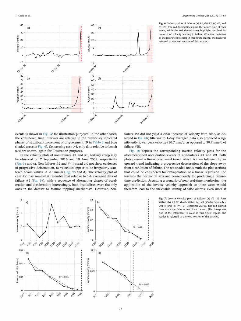
events is shown in Fig. 9c for illustration purposes. In the other cases,the considered time intervals are relative to the previously indicatedphases of significant increment of displacement (D in Table 3 and blueshaded areas in Fig. 4). Concerning case #4, only data relative to bench070 are shown, again for illustration purposes.

In the velocity plots of non-failures #1 and #3, tertiary creep maybe observed on 7 September 2016 and 19 June 2008, respectively(Fig. 9a and c). Non-failures #2 and #4 instead did not show evidencesof progressive deformation, as velocities appear to be irregularly scat-tered across values < 2.5 mm/h (Fig. 9b and d). The velocity plot ofcase #2 may somewhat resemble that relative to 1-h averaged data offailure #5 (Fig. 8a), with a sequence of alternating phases of accel-eration and deceleration; interestingly, both instabilities were the onlyones in the dataset to feature toppling mechanism. However, non-

failure #2 did not yield a clear increase of velocity with time, as de-tected in Fig. 8b; filtering to 1-day averaged data also produced a sig-nificantly lower peak velocity (10.7 mm/d, as opposed to 30.7 mm/d offailure #5).

Fig. 10 depicts the corresponding inverse velocity plots for theaforementioned acceleration events of non-failures #1 and #3. Bothplots present a linear downward trend, which is then followed by anupward trend indicating a progressive deceleration of the slope awayfrom a condition of failure. The red shaded areas mark the plot sectionsthat could be considered for extrapolation of a linear regression linetowards the horizontal axis and consequently for producing a failure-time prediction. Assuming a scenario of near real-time monitoring, theapplication of the inverse velocity approach to these cases wouldtherefore lead to the inevitable issuing of false alarms, even more if

-10

0

10

20

30

40

Vel

ocity

(m

m/h

)

-10

0

10

20

30

40

Vel

ocity

(m

m/h

)

-10

0

10

20

30

40

50

60

70

Vel

ocity

(m

m/h

)

-10

0

10

20

30

40

50

60

70

80

Vel

ocity

(m

m/h

)

a)

c)

b)

d)

Fig. 6. Velocity plots of failures (a) #1, (b) #2, (c) #3, and(d) #4. The red dashed lines mark the failure-time of eachevent, while the red shaded areas highlight the final in-crement of velocity leading to failure. (For interpretationof the references to color in this figure legend, the reader isreferred to the web version of this article.)

0

0.2

0.4

0.6

Inve

rse

velo

city

(h/

mm

)

0

0.05

0.1

Inve

rse

velo

city

(h/

mm

)

R² = 0.95

R² = 0.97

R² = 0.95

0

0.2

0.4

0.6

0.8

Inve

rse

velo

city

(h/

mm

)

-6

0

6

12

Inve

rse

velo

city

(h/

mm

)

a)

c)

b)

d)

Fig. 7. Inverse velocity plots of failures (a) #1 (13 June2016), (b) #2 (7 March 2014), (c) #3 (25–26 September2014), and (d) #4 (21 December 2016). The red dashedlines mark the failure-time of each event. (For interpreta-tion of the references to color in this figure legend, thereader is referred to the web version of this article.)

T. Carlà et al. Engineering Geology 228 (2017) 71–81

76

considering the significant rates of slope movement associated withthese tertiary creep phases (peak velocities of 10 mm/h and 25.3 mm/hin non-failures #1 and #3, respectively).

4. Discussion

Several useful inputs regarding slope failure predictability, and therequisites that are necessary to implement effective monitoring pro-grams and early warning systems, may be derived from the presentedradar data. In particular, these apply to the risk mitigation in slopes thatare potentially affected by rapid accelerations.

4.1. Temporal evolution of the displacements and tertiary creep

Increments of the slope displacements in the pit can be sudden andextremely rapid: in particular, failures #1–#4 were all anticipated byaccelerations that lasted for only few hours (Figs. 2 and 6), whilenegligible amounts of deformation were measured before their re-spective onset. Within the context of significantly longer phases of de-formation (i.e. several days to several months), brief accelerations ofsimilar nature were occasionally associated to non-failures as well (seecases #1 and #3 in Fig. 4a and c). The toppling failure #5 experienced

a precursor deformation with a somewhat intermediate behavior be-tween the rapid movements of failures #1–#4 and the prolongedphases of deformation of the other non-failure case studies.

Interestingly, these accelerations may be related to phases of ter-tiary creep. Data from failure #1, which featured the most rapid of theobserved events of acceleration in the dataset (Fig. 6a), did not showclear progressive deformation arguably because of the inadequacy ofthe 20-min sampling rate by which this instability was monitored. Theapparent lack of tertiary creep prior to brittle failure in hard rockmasses, as described by Rose and Hungr (2007), is thus likely to berelated to an issue of too low frequency of measurement acquisition,and not to a different slope kinematics.

4.2. LOS sensitivity

The impact of the LOS assumes pivotal importance, as an incorrectdata correction may decisively alter the perception of the displacements(Table 1). By knowing the positions of the radar and of the instability,along with the actual direction of slope movement, the correction of themeasurements according to the radar sensitivity is a simple procedure.However, this is much less easily obtained at the scale of an open-pitmine, where instabilities may be numerous and have widely differentcharacteristics; in addition to this point, the geometry and aspect of therock faces frequently change in consequence of the continuous ex-cavation works. The above applies even more to the monitoring of hardrock masses, where failures may develop very rapidly and thus givelittle time to assess mechanism and kinematics of movement. Given thatinstabilities in such a context are typically structurally controlled, theideal solution would be to use a map of the expected direction ofmovement of all the sectors of the pit covered by the radar (e.g. bymeans of a 3D kinematic analysis Gokceoglu et al., 2000; Gigli et al.,2012; Fanti et al., 2013; Gigli et al., 2014), to calculate the sensitivity ofthe radar LOS to those directions, and then to define alarm thresholdsbased on monitoring data corrected according to the LOS sensitivity.

-1

0

1

2

3

4

Vel

ocity

(m

m/h

)

R² = 0.82

0

0.1

0.2

0.3

Inve

rse

velo

city

(d/

mm

)

0

1

2

3

4

Inve

rse

velo

city

(h/

mm

)

-5

0

5

10

15

20

25

30

35

Vel

ocity

(m

m/d

)

a)

c)

b)

d)

Fig. 8. Failure #5: (a) 1-h averaged velocity, (b) 1-day averaged velocity, (c) 1-h averaged inverse velocity (5 February 2017), and (d) 1-day averaged inverse velocity. The red dashedlines mark the failure-time. (For interpretation of the references to color in this figure legend, the reader is referred to the web version of this article.)

Table 3Characteristics of non-failures #1, #2, #3, and #4.

Case Mechanism Estimated mass(t)

D (days)* Actual vp(mm/h)**

Actual ap(mm/h^2)**

#1 Planar 35,000 9 10 7.4#2 Toppling 7500 13 2.3 1.2#3 Wedge 92,000 270 25.3 14.9#4 Wedge 750,000 205 1.9 1.4

D = Duration of significant increment of displacement that did not lead to failure (blueshaded areas in Fig. 4);* vp = peak velocity;** ap = peak acceleration.***Derived from raw monitoring data (Fig. 4). **Derived from 1-h averaged data (Fig. 9).

T. Carlà et al. Engineering Geology 228 (2017) 71–81

77

4.3. Mechanism

With regards to the mechanism of the instabilities, planar andwedge modes did not show obvious reciprocal differences in terms oftrends of displacement. Conversely, a peculiar behavior was observedfor the two toppling instabilities in the dataset (the effects of noiseinduced by the ongoing production works on the displacement mea-surements of failure #5 were unclear; however, given the evident si-milarities with data of non-failure #2, it is inferred that these were notsignificant). In both instances the main phase of slope deformation sawin fact the occurrence of lower rates of displacement, and of an alter-nation of accelerations and decelerations (Figs. 8a and 9b). This may beexplained as follows: while planar and wedge instabilities involve re-lative movement between rock blocks with respect to one or morediscontinuities, on the other hand a toppling mechanism implies theopening of a controlling sub-vertical fracture, and therefore the cyclicalincrease and decrease of velocity may reflect this process as it developsintermittently with time. In both cases of toppling, the displacements

might also have been influenced by the excavation activities that weretaking place in the area: the mine staff reported that acceleration of theslope was mostly observed as material was removed, whereas decel-eration occurred when mining was stopped. Still, regardless of thecause, and although requiring additional data smoothing, it was pos-sible to extrapolate tertiary creep behavior in the precursor displace-ments of failure #5.

4.4. “Signature” of the failure events

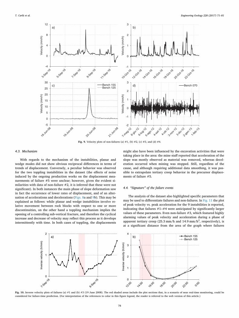
The analysis of the dataset also highlighted specific parameters thatmay be used to differentiate failures and non-failures. In Fig. 11 the plotof peak velocity vs. peak acceleration for the 9 instabilities is reported,indicating that failures #1–#4 were anticipated by significantly largervalues of these parameters. Even non-failure #3, which featured highlyalarming values of peak velocity and acceleration during a phase ofapparent tertiary creep (25.3 mm/h and 14.9 mm/h2, respectively), isat a significant distance from the area of the graph where failures

-2

-1

0

1

2

3

Vel

ocity

(m

m/h

)

Bench 070

-5

0

5

10

15

20

25

30

Vel

ocity

(m

m/h

)

Bench 155Bench 125

-4

0

4

8

12

Vel

ocity

(m

m/h

)

-1

0

1

2

3

Vel

ocity

(m

m/h

)

a)

c)

b)

d)

Fig. 9. Velocity plots of non-failures (a) #1, (b) #2, (c) #3, and (d) #4.

0

1

2

3

4

Inve

rse

velo

city

(h/

mm

)

Bench 155Bench 125

0

1

2

Inve

rse

velo

city

(h/

mm

)

a) b)

Fig. 10. Inverse velocity plots of failures (a) #1 and (b) #3 (19 June 2008). The red shaded areas include the plot sections that, in a scenario of near real-time monitoring, could beconsidered for failure-time prediction. (For interpretation of the references to color in this figure legend, the reader is referred to the web version of this article.)

T. Carlà et al. Engineering Geology 228 (2017) 71–81

78

#1–#4 are located. A threshold separating the two groups may bepreliminarily defined around values of 30 mm/h and 20 mm/h2. Thetwo toppling instabilities are both identified in the lower left part of thegraph; this may be associated with the different characteristics of theirdeformation behavior, as previously described. Even so, it is worthnoting that the toppling failure was anticipated by greater peak velocityand acceleration with respect to the toppling non-failure. This in-troduces a possible additional level of discrimination for the phase ofearly warning, as it may be convenient to define specific alarmthresholds on the basis of the failure mechanism.

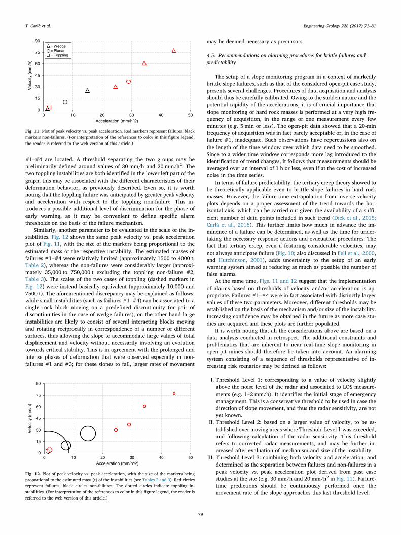
Similarly, another parameter to be evaluated is the scale of the in-stabilities. Fig. 12 shows the same peak velocity vs. peak accelerationplot of Fig. 11, with the size of the markers being proportional to theestimated mass of the respective instability. The estimated masses offailures #1–#4 were relatively limited (approximately 1500 to 4000 t,Table 2), whereas the non-failures were considerably larger (approxi-mately 35,000 to 750,000 t excluding the toppling non-failure #2,Table 3). The scales of the two cases of toppling (dashed markers inFig. 12) were instead basically equivalent (approximately 10,000 and7500 t). The aforementioned discrepancy may be explained as follows:while small instabilities (such as failures #1–#4) can be associated to asingle rock block moving on a predefined discontinuity (or pair ofdiscontinuities in the case of wedge failures), on the other hand largeinstabilities are likely to consist of several interacting blocks movingand rotating reciprocally in correspondence of a number of differentsurfaces, thus allowing the slope to accommodate large values of totaldisplacement and velocity without necessarily involving an evolutiontowards critical stability. This is in agreement with the prolonged andintense phases of deformation that were observed especially in non-failures #1 and #3; for these slopes to fail, larger rates of movement

may be deemed necessary as precursors.

4.5. Recommendations on alarming procedures for brittle failures andpredictability

The setup of a slope monitoring program in a context of markedlybrittle slope failures, such as that of the considered open-pit case study,presents several challenges. Procedures of data acquisition and analysisshould thus be carefully calibrated. Owing to the sudden nature and thepotential rapidity of the accelerations, it is of crucial importance thatslope monitoring of hard rock masses is performed at a very high fre-quency of acquisition, in the range of one measurement every fewminutes (e.g. 5 min or less). The open-pit data showed that a 20-minfrequency of acquisition was in fact barely acceptable or, in the case offailure #1, inadequate. Such observations have repercussions also onthe length of the time window over which data need to be smoothed.Since to a wider time window corresponds more lag introduced to theidentification of trend changes, it follows that measurements should beaveraged over an interval of 1 h or less, even if at the cost of increasednoise in the time series.

In terms of failure predictability, the tertiary creep theory showed tobe theoretically applicable even to brittle slope failures in hard rockmasses. However, the failure-time extrapolation from inverse velocityplots depends on a proper assessment of the trend towards the hor-izontal axis, which can be carried out given the availability of a suffi-cient number of data points included in such trend (Dick et al., 2015;Carlà et al., 2016). This further limits how much in advance the im-minence of a failure can be determined, as well as the time for under-taking the necessary response actions and evacuation procedures. Thefact that tertiary creep, even if featuring considerable velocities, maynot always anticipate failure (Fig. 10; also discussed in Fell et al., 2000,and Hutchinson, 2001), adds uncertainty to the setup of an earlywarning system aimed at reducing as much as possible the number offalse alarms.

At the same time, Figs. 11 and 12 suggest that the implementationof alarms based on thresholds of velocity and/or acceleration is ap-propriate. Failures #1–#4 were in fact associated with distinctly largervalues of these two parameters. Moreover, different thresholds may beestablished on the basis of the mechanism and/or size of the instability.Increasing confidence may be obtained in the future as more case stu-dies are acquired and these plots are further populated.

It is worth noting that all the considerations above are based on adata analysis conducted in retrospect. The additional constraints andproblematics that are inherent to near real-time slope monitoring inopen-pit mines should therefore be taken into account. An alarmingsystem consisting of a sequence of thresholds representative of in-creasing risk scenarios may be defined as follows:

I. Threshold Level 1: corresponding to a value of velocity slightlyabove the noise level of the radar and associated to LOS measure-ments (e.g. 1–2 mm/h). It identifies the initial stage of emergencymanagement. This is a conservative threshold to be used in case thedirection of slope movement, and thus the radar sensitivity, are notyet known.

II. Threshold Level 2: based on a larger value of velocity, to be es-tablished over moving areas where Threshold Level 1 was exceeded,and following calculation of the radar sensitivity. This thresholdrefers to corrected radar measurements, and may be further in-creased after evaluation of mechanism and size of the instability.

III. Threshold Level 3: combining both velocity and acceleration, anddetermined as the separation between failures and non-failures in apeak velocity vs. peak acceleration plot derived from past casestudies at the site (e.g. 30 mm/h and 20 mm/h2 in Fig. 11). Failure-time predictions should be continuously performed once themovement rate of the slope approaches this last threshold level.

0

15

30

45

60

75

90

0 10 20 30 40 50

Vel

ocity

(m

m/h

)

Acceleration (mm/h^2)

= Wedge= Planar= Toppling

Fig. 11. Plot of peak velocity vs. peak acceleration. Red markers represent failures, blackmarkers non-failures. (For interpretation of the references to color in this figure legend,the reader is referred to the web version of this article.)

0

15

30

45

60

75

90

0 10 20 30 40 50

Vel

ocity

(m

m/h

)

Acceleration (mm/h^2)

Fig. 12. Plot of peak velocity vs. peak acceleration, with the size of the markers beingproportional to the estimated mass (t) of the instabilities (see Tables 2 and 3). Red circlesrepresent failures, black circles non-failures. The dotted circles indicate toppling in-stabilities. (For interpretation of the references to color in this figure legend, the reader isreferred to the web version of this article.)

T. Carlà et al. Engineering Geology 228 (2017) 71–81

79

Finally, it can be evinced that the mitigation of slope failure risk isnot to be performed according to a black box approach, i.e. by acquiringand analyzing data without any knowledge on the specific issues relatedto the monitored scenario. The latter observation applies to both open-pit mine operations and natural slopes. In particular, the setup of ef-fective monitoring programs and early warning systems is strictly de-pendent on their appropriate calibration and contextualization in theframe of the on-site characteristics and deformation behavior. While tothis point the geomechanical properties of the rock mass can give ageneral indication, the back-analysis of monitoring data from past slopeinstabilities (assuming their availability) is of crucial importance. Sincethe nature of the slope deformation may also vary depending on severalother factors, as many complementary data as possible need to becollected and reviewed.

5. Conclusions

The mitigation of slope failure risk is an essential part of the safetystrategies in open-pit mines. Studying the typical slope deformationbehavior in the pit is crucial to the setup of monitoring programs andearly warning systems, and in this sense considerable insight may begained by reviewing monitoring data relative to past cases of in-stability.

The analysis of radar monitoring data from 9 cases of instability atan undisclosed open-pit mine provided the opportunity to analyze indetail the deformation of hard rock masses subject to markedly brittlefailure. The goal of such an analysis was to define the characteristics ofthe slope movements in the pit and the appropriate strategy for thesetup of alarms. This also allowed to assess whether, as opposed to thecommon perception, it is possible to effectively predict and managebrittle slope failures by evaluating the trend of the precursor de-formation. Adding to this topic, another point of interest was to sepa-rately characterize the failures from the cases of instability that, al-though showing considerable displacements, ultimately did not evolveinto failure (“non-failures”), and consequently to define a sort of “sig-nature” of the failure events.

The results showed that tertiary creep indeed affects also rock slopesof high geomechanical quality, and that it may develop very rapidly ona scale of a few hours. This has obvious repercussions in terms of fre-quency of measurement acquisition and reference interval of the dataprocessing that are needed in order to successfully predict failures andprovide sufficient notice for the necessary response actions and eva-cuation procedures. The case studies were also considered in terms ofpeak velocity and acceleration, following which it was determined thatthe failures were anticipated by significantly larger values of these twoparameters.

It was observed that other factors possibly influencing the slopedeformation behavior and tendency to failure are the size and me-chanism of the instability. In particular, failures #1–#4 were all ofrelatively small size (estimated mass of 4000 t or less), whereas non-failures were typically 1 or more order of magnitudes larger. In acontext of near real-time slope monitoring, it is then essential to take indue consideration also these (and possibly other) parameters, as it maybe convenient to set different alarm thresholds depending on geometryand properties of the detected slope movement. Strictly related to allthe above is the importance to account for the variable radar LOSsensitivity across the pit, as uncorrected measurements of displacementmay point to highly misleading observations and to a false perception ofthe inherent risk.

It is concluded that any slope monitoring program and earlywarning system is effective only if calibrated and contextualized in theframe of the on-site slope characteristics and deformation behavior.Such consideration is deemed to be valid for the mitigation of slopefailure risk in both artificial and natural slopes.

References

Antonello, G., Casagli, N., Farina, P., Leva, D., Nico, G., Sieber, A.J., Tarchi, D., 2004.Ground-based SAR interferometry for monitoring mass movements. Landslides 1 (1),21–28.

Armstrong, J., Rose, N.D., 2009. Mine operation and management of progressive slopedeformation on the south wall of the Barrick Goldstrike Betze-Post Open Pit. In:Proceedings of Slope Stability 2009: International Symposium on Rock Slope Stabilityin Open Pit Mining and Civil Engineering, Santiago.

Atzeni, C., Barla, M., Pieraccini, M., Antolini, F., 2015. Early warning monitoring ofnatural and engineered slopes with ground-based synthetic-aperture radar. RockMech. Rock. Eng. 48 (1), 235–246.

Bardi, F., Raspini, F., Frodella, W., Lombardi, L., Nocentini, M., Gigli, G., Morelli, S.,Corsini, A., Casagli, N., 2017. Monitoring the rapid-moving reactivation of earthflows by means of GB-InSAR: the April 2013 Capriglio landslide (NorthernAppenines, Italy). Remote Sens. 9 (2), 165.

Carlà, T., Intrieri, E., Di Traglia, F., Nolesini, T., Gigli, G., Casagli, N., 2016. Guidelines onthe use of inverse velocity method as a tool for setting alarm thresholds and fore-casting landslides and structure collapses. Landslides in press. http://dx.doi.org/10.1007/s10346-016-0731-5.

Casagli, N., Catani, F., Del Ventisette, C., Luzi, G., 2010. Monitoring, prediction, and earlywarning using ground-based radar interferometry. Landslides 7 (3), 291–301.

Casagli, N., Frodella, W., Morelli, S., Tofani, V., Ciampalini, A., Intrieri, E., Raspini, F.,Rossi, G., Tanteri, L., Lu, P., 2017. Spaceborne, UAV and ground-based remote sen-sing techniques for landslide mapping, monitoring and early warning. Geoenviron.Disaster 4 (9), 1–23.

Crosta, G.B., Agliardi, F., 2002. How to obtain alert velocity thresholds for large rock-slides. Phys. Chem. Earth 27, 1557–1565.

Di Traglia, F., Nolesini, T., Intrieri, E., Mugnai, F., Leva, D., Rosi, M., Casagli, N., 2014.Review of ten years of volcano deformations recorded by the ground-based InSARmonitoring system at Stromboli volcano: a tool to mitigate volcano flank dynamicsand intense volcanic activity. Earth-Sci. Rev. 139, 317–335.

Dick, G.J., Eberhardt, E., Cabrejo-Liévano, A.G., Stead, D., Rose, N.D., 2015. Developmentof an early-warning time-of-failure analysis methodology for open-pit mine slopesutilizing ground-based slope stability radar monitoring data. Can. Geotech. J. 52 (4),515–529.

Doyle, J.B., Reese, J.D., 2011. Slope monitoring and back analysis of east fault failure,Bingham Canyon Mine, Utah. In: Proceedings of Slope Stability 2011: InternationalSymposium on Rock Slope Stability in Open Pit Mining and Civil Engineering.Canadian Rock Mechanics Association, Vancouver, BC.

Eberhardt, E., Stead, D., Coggan, J.S., 2004. Numerical analysis of initiation and pro-gressive failure in natural slopes – the 1991 Randa rockslide. Int. J. Rock Mech. Min.Sci. 41, 69–87.

Fanti, R., Gigli, G., Lombardi, L., Tapete, D., Canuti, P., 2013. Terrestrial laser scanningfor rockfall stability analysis in the cultural heritage site of Pitigliano (Italy).Landslides 10 (4), 409–420.

Farina, P., Coli, N., Yön, R., Eken, G., Keitzmen, H., 2013. Efficient real time stabilitymonitoring of mine walls: the Çöllolar Mine Case Study. In: Proceedings of the 23rdInternational Mining Congress & Exhibition of Turkey, Antalya, Turkey, pp. 111–117.

Farina, P., Coli, N., Coppi, F., Babboni, F., Leoni, L., Marques, T., Costa, F., 2014. Recentadvances in slope monitoring radar for open-pit mines. In: Proceedings of MineClosure Solutions 2014, Ouro Preto, Minas Gerais, Brazil, (ISBN: 978-0-9917905-4-8).

Federico, A., Popescu, M., Elia, G., Fidelibus, C., Internò, G., Murianni, A., 2012.Prediction of time to slope failure: a general framework. Environ. Earth Sci. 66,245–256.

Fell, R., Hungr, O., Leroueil, S., Riemer, W., 2000. Geotechnical engineering of the sta-bility of natural slopes and cuts and fills in soil. In: Proceedings of the InternationalConference on Geotechnical and Geological Engineering, Melbourne, pp. 21–120.

Fukuzono, T., 1985. A new method for predicting the failure time of a slope. In:Proceedings of the 4th International Conference and Field Workshop on Landslides,Tokyo, pp. 145–150.

Gigli, G., Frodella, W., Mugnai, F., Tapete, D., Cigna, F., Fanti, R., Intrieri, E., Lombardi,L., 2012. Instability mechanisms affecting cultural heritage sites in the Maltese ar-chipelago. Nat. Hazards Earth Syst. Sci. 12, 1883–1903.

Gigli, G., Morelli, S., Fornera, S., Casagli, N., 2014. Terrestrial laser scanner and geo-mechanical surveys for the rapid evaluation of rock fall susceptibility scenarios.Landslides 11 (1), 1–14.

Ginting, A., Stawski, M., Widiadi, R., 2011. Geotechnical risk management and mitigationat Grasberg Open Pit, PT Freeport Indonesia. In: Proceedings of Slope Stability 2011:International Symposium on Rock Slope Stability in Open Pit Mining and CivilEngineering, Canadian Rock Mechanics Association, Vancouver, BC.

Gokceoglu, C., Sonmez, H., Ercanoglu, M., 2000. Discontinuity controlled probabilisticslope failure risk maps of the Altindag (settlement) region in Turkey. Eng. Geol. 55,277–296.

Hutchinson, J., 2001. Landslide risk – to know, to foresee, to prevent. Geologia TecnicaAmbientale 9, 3–24.

Intrieri, E., Gigli, G., 2016. Landslide forecasting and factors influencing predictability.Nat. Hazards Earth Syst. Sci. 75 (24), 2501–2510.

Intrieri, E., Gigli, G., Casagli, N., Nadim, F., 2013. Brief communication “landslide earlywarning system: toolbox and general concepts”. Nat. Hazards Earth Syst. Sci. 13,85–90.

Lacasse, S., Nadim, F., 2009. Landslide risk assessment and mitigation strategy. In:Landslides – disaster risk reduction. Springer, Berlin Heidelberg, pp. 31–61.

Luzi, G., Pieraccini, M., Mecatti, D., Noferini, L., Macaluso, G., Galgaro, A., Atzeni, C.,

T. Carlà et al. Engineering Geology 228 (2017) 71–81

80

2006. Advances in ground based microwave interferometry for landslide survey: acase study. Int. J. Remote Sens. 27 (12), 2331–2350.

Macciotta, R., Hendry, M., Martin, C.D., 2016. Developing an early warning system for avery slow landslide based on displacement monitoring. Nat. Hazards 81 (2), 887–907.

Macqueen, G.K., Salas, E.I., Hutchison, B.J., 2013. Application of radar monitoring atSavage River Mine, Tasmania. In: Proceedings of Slope Stability 2013: InternationalSymposium on Rock Slope Stability in Open Pit Mining and Civil Engineering,Australian Centre for Geomechanics, Brisbane, Australia.

Monserrat, O., Crosetto, M., Luzi, G., 2014. A review of ground-based SAR interferometryfor deformation measurement. ISPRS J. Photogramm. Remote Sens. 93, 40–48.

Morales, M., Panthi, K., Botsialas, K., Holmøy, K.H., 2017. Development of a 3D structuralmodel of a mine by consolidating different data sources. Bull. Eng. Geol. Environ.http://dx.doi.org/10.1007/s10064-017-1068-6.

Paronuzzi, P., Bolla, A., Rigo, E., 2016. Brittle and ductile behavior in deep-seated

landslides: learning from the Vajont experience. Rock Mech. Rock. Eng. 49,2389–2411.

Read, J., Stacey, P., 2009. Guidelines for Open Pit Slope Design. CSIRO Publishing,Australia.

Rose, N.D., Hungr, O., 2007. Forecasting potential rock slope failure in open pit minesusing the inverse-velocity method. Int. J. Rock Mech. Min. Sci. 44, 308–320.

Vaziri, A., Moore, L., Ali, H., 2010. Monitoring systems for warning impending failures inslopes and open pit mines. Nat. Hazards 55 (2), 501–512.

Voight, B., 1988. A method for prediction of volcanic eruptions. Nature 332, 125–130.Voight, B., 1989. A relation to describe rate-dependent material failure. Science 243,

200–203.Zavodni, Z.M., Broadbent, C.D., 1980. Slope failure kinematics. Bull. Can. Inst. Min. 73

(816), 69–74.

T. Carlà et al. Engineering Geology 228 (2017) 71–81

81