On the polarizability and capacitance of the cube

Johan Helsing∗, Karl-Mikael Perfekt

Centre for Mathematical SciencesLund University, Box 118, SE-221 00 Lund, Sweden

Abstract

An efficient integral equation based solver is constructed for the electrostatic problem on domainswith cuboidal inclusions. It can be used to compute the polarizability of a dielectric cube ina dielectric background medium at virtually every permittivity ratio for which it exists. Forexample, polarizabilities accurate to between five and ten digits are obtained (as complex limits)for negative permittivity ratios in minutes on a standard workstation. In passing, the capacitanceof the unit cube is determined with unprecedented accuracy. With full rigor, we develop a naturalmathematical framework suited for the study of the polarizability of Lipschitz domains. Severalaspects of polarizabilities and their representing measures are clarified, including limiting behaviorboth when approaching the support of the measure and when deforming smooth domains into anon-smooth domain. The success of the mathematical theory is achieved through symmetrizationarguments for layer potentials.

Keywords: electrostatic boundary value problem, Lipschitz domain, polarizability, capacitance,spectral measure, layer potential, continuous spectrum, Sobolev space, multilevel solver, cube

1. Introduction

The determination of polarizabilities and capacitances of inclusions of various shapes has a longhistory in computational electromagnetics. Inclusions with smooth surfaces are, by now, ratherstandard to treat. When surfaces are non-smooth, however, the situation is different. Numericalsolvers can run into problems related to stability and resolution. Particularly so in three dimensionsand for certain permittivity combinations. Solutions may not converge or results could be hard tointerpret. See [44, 45, 51] and references therein. The situation on the theoretical side is similar.When, and in what sense do solutions exist? Such questions are in the mainstream of contemporaryresearch in harmonic analysis. Coincidentally, also in applied physics (plasmonics) there is agrowing interest in solving electrostatic problems on domains with structural discontinuities and aconcern about the sufficiency of available solvers [19, 54].

This paper addresses several fundamental issues related to the problems just mentioned. Weconstruct a stable solver for the polarizability and capacitance of a cube based on an integralequation using the adjoint of the double layer potential. We compute solutions of unprecedentedaccuracy and interpret the results within a rigorous mathematical framework. The reason for

∗Corresponding author, Tel.:+46 46 2223372.Email addresses: helsing@maths.lth.se (Johan Helsing), perfekt@maths.lth.se (Karl-Mikael Perfekt)

Published in Appl. Comput. Harmon. Anal., vol. 34, pp. 445–468, 2013. (typos corrected October 14, 2016)

working with a cube are twofold. First, the cube has the advantage that its geometric difficultiesare concentrated to edges and corners, since its faces are flat. Integral equation techniques, whichoften excel for boundary value problems in two dimensions, typically suffer from loss of accuracy inthe discretization of weakly singular integral operators on curved surfaces in three dimensions. Herewe need not worry about that. Secondly, cubes are actually common in plasmonic applications.

In the purely theoretical sections we begin by collecting a number of results and recent advancesin the theory of layer potentials associated with the Laplacian in Lipschitz domains. The mostobvious reason for this is that the invertibility study of layer potentials leads to the solution ofthe boundary value problem implicit in the definition of polarizability, and is as such the basisfor both the mathematical and numerical aspects of this paper. Furthermore, the properties ofthe polarizability for a non-smooth domain such as a cube are quite subtle, and it is our ambitionto provide a solid theoretical foundation for the problem at hand, giving a careful and detailedexposition of a mathematical framework that clarifies a number of points.

Since the double layer potential is not self-adjoint in the L2-pairing, we develop certain sym-metrization techniques for it, in particular extending the work of Khavinson, Putinar and Shapiro[31] to the case of a non-smooth domain. These techniques are used to prove the unique existence ofthe polarizability itself for a Lipschitz domain, as well as of a corresponding representing measure[18]. We present a thorough discussion of the smooth case, the limiting behavior in passing fromthe smooth to the non-smooth case, and ultimately the general case. Concerning the last point,a condition ensuring that the representing measure has no singular part is given, and it is proventhat in the support of the absolutely continuous part of the measure, the polarizability can not begiven a direct interpretation in terms of a potential with finite energy solving the related boundaryvalue problem.

The paper is organized as follows: Section 2 formulates the electrostatic problem and defines thepolarizability. Existence issues and representations are reviewed in Section 3. For ease of reading,rigorous statements and proofs are deferred to Sections 4 and 5. The capacitance is discussed inSection 6. Section 7 reviews the state of the art with regard to numerical schemes. Section 8 givesa necessary background to the present solver. New development takes place in Section 9. The lastsections contain numerical examples performed in Matlab. Section 10 illustrates the effects ofrounding corners and Section 11 is about the cube.

The main conclusion of the paper is that, from a numerical viewpoint, it is an advantage to letcubes have sharp edges and corners as opposed to the common practice of rounding them slightly.Furthermore, the representing measure for the polarizability of the cube is determined, and a newbenchmark for the capacitance of the unit cube is established.

2. The electrostatic problem and the polarizability

Let a domain V , an inclusion with surface S and permittivity ε2, be embedded in an infinitespace. The exterior to the closure of V is denoted E and has permittivity ε1. Let νr be the exteriorunit normal of S at position r.

We seek a potential U(r), continuous in E ∪ S ∪ V , which satisfies the electrostatic equation

−∆U(r) = 0 , r ∈ E ∪ V , (1)

subject to the boundary conditions on the limits of normal derivatives

ε1∂

∂νrU ext(r) = ε2

∂

∂νrU int(r) (2)

2

and behavior at infinitylimr→∞

∇U(r) = e . (3)

Here superscripts ext and int denote limits from the exterior or interior of S, respectively, and e isan applied unit field. Eqs. (1), (2), (3) constitute a partial differential equation formulation of theelectrostatic problem. Proposition 5.1 gives a strict interpretation of what it means for a potentialU(r) to solve this problem, in particular expressing (2) in a distribution sense.

For the construction of solutions to (1), (2), (3) we make use of fundamental solutions to theLaplace equation in two and three dimensions

G(r, r′) = − 1

2πlog |r − r′| and G(r, r′) =

1

4π

1

|r − r′|, (4)

and represent U(r) in terms of a single layer density ρ(r) as

U(r) = e · r +

∫SG(r, r′)ρ(r′) dσr′ , (5)

where dσ is an element of surface area.The representation (5) satisfies (1) and (3). Its insertion in (2) gives the integral equation for

ρ(r)

ρ(r) + 2λ

∫S

∂

∂νrG(r, r′)ρ(r′) dσr′ = −2λ (e · νr) , r ∈ S , (6)

where the parameter

λ =ε2 − ε1ε2 + ε1

. (7)

The polarizability tensor of V can be defined in terms of an integral over a polarization field.When V features sufficient symmetry, such as the octahedral symmetry of the cube, the polariz-ability is isotropic and reduces to a scalar α(ε1, ε2), see [48], which can be determined via

(ε2 − ε1)

∫V∇U(r) dr = α(ε1, ε2)e , (8)

where dr is a volume element. Using integration by parts in (8) it is possible to express α(ε1, ε2)as an integral over ρ(r)

α(ε1, ε2) = −ε1∫Sρ(r) (e · r) dσr . (9)

More generally, the components of the polarizability tensor can be recovered via integrals similarto that in (9) using different applied fields e, but in what follows we tacitly assume that V issufficiently symmetric as to allow for a scalar valued α(ε1, ε2).

3. Theory – overview

For what surface shapes S and permittivities ε1, ε2 does the electrostatic problem have asolution? Starting with (6) and partly following [37], this section sketches the derivation of someimportant existence results. It also motivates an integral representation formula for α(ε1, ε2) andtwo sum rules which are used for validation in our numerical experiments.

3

3.1. Existence of solutions for smooth S

Let us rewrite (6) in the abbreviated form

(I + λK) ρ(r) = λg(r) , (10)

where I is the identity. If S is smooth, then (10) is a Fredholm second kind integral equationwith a compact, non-self adjoint, integral operator K whose spectrum is discrete and accumulatesat zero. Let K and its adjoint K∗ (the double layer potential) have eigenvectors φi and ψi withcorresponding eigenvalues zi. All eigenvalues are real and bounded by one in modulus. Non-zeroeigenvalues have finite multiplicities. Normalizing∫

Sψi(r)φj(r) dσr = δij , (11)

the kernel of K can be written

K(r, r′) =∑i

ziφi(r)ψi(r′) . (12)

See, further, the discussion in Section 5.2.Let us introduce a new variable z and a scaled polarizability α(z) as

z = −1/λ , (13)

α(z) ≡ α(ε1, ε2)

|V |ε1, (14)

where |V | is the volume of V . Then (14), with (9), can be written in the abbreviated form

α(z) =

∫Sh(r)ρ(r) dσr . (15)

The relation (13) allows us to use the parameter λ or its negative reciprocal z, depending on whatis most convenient in a given situation.

In terms of the quantities

ui =

∫Sh(r)φi(r) dσr and vi =

∫Sψi(r)g(r) dσr , (16)

and using (12) to construct the resolvent of (10), one can write

ρ(r) =∑i

φi(r)vizi − z

(17)

andα(z) =

∑i

uivizi − z

, (18)

see Theorem 5.6. This suggests that neither U(r) nor α(z) exists for z = zi when uivi 6= 0. Thereis an electrostatic resonance or plasmon at zi.

For ease of interpretation, the sum in (18) can be considered as taken over distinct eigenvaluesand with uivi, for a degenerate eigenvalue, being the sum of all residues belonging to that eigenvalue.

4

Then all uivi are non-negative and plasmons can be classified as bright or dark depending on whetheruivi > 0 or not [54]. When S is a circle, there are only two eigenvalues: z1 = −1 which is simpleand corresponds to a dark plasmon and z2 = 0 which has infinite multiplicity and corresponds toa bright plasmon. When S is a sphere, the eigenvalues are zi = 1/(1− 2i). The multiplicity of ziis 2i− 1. The only bright plasmon is associated with z2.

For later reference we observe that the sum of all residues is∑i

uivi =

∫Sh(r)g(r) dσr = 2 . (19)

When the polarizability is isotropic one can, using techniques from [15], also derive a weighted sumrule ∑

i

ziuivi =

∫S

∫Sh(r)K(r, r′)g(r′) dσ′r dσr = 2(2/d− 1) , (20)

where d = 2, 3 is the dimension.

3.2. Existence of solutions for non-smooth S

If S is gradually transformed from a smooth surface into a non-smooth surface, eigenvalueszi travel and occupy a certain subset of the interval [−1, 1] ever more densely. When S ceasesto be smooth, K is no longer compact with discrete eigenvalues. Rather, K has a continuousspectrum which on a certain function space coincides with the aforementioned subset, accompaniedby discrete values. Disregarding the discrete spectrum, which for squares and cubes turns out tocorrespond to dark plasmons, the sum (18) assumes a limit

α(z) =

∫R

dµ(x)

x− z=

∫σµ

µ′(x) dx

x− z, (21)

where the measure µ(x) is real and non-negative and σµ = {x : µ′(x) > 0}. Here we have ignoredthe possible presence of a singular spectrum. For further details and a condition that serves toexclude this complication, see Theorems 5.2 and Section 5.2. The sum rules (19) and (20) assumethe forms ∫

Rµ′(x) dx = 2 , (22)∫

Rxµ′(x) dx = 2(2/d− 1) . (23)

The numerical results in Sections 10 and 11 suggest that both the square and the cube haveσµ equal to a single, possibly punctured, interval (a, b) ⊂ [−1, 1]. The square has a = −0.5 andb = 0.5, consistent with the exact computations of the spectral radius for a square found in [35]and [53]. The cube has a ≈ −0.694526 and b = 0.5. For later reference we let σµsq denote σµ ofthe square and σµcu denote σµ of the cube.

For a large class of non-smooth S, the potential U(r) exists when z stays away from a certaincompact set L : σµ ⊂ L ⊂ [−1, 1]. Furthermore, α(z) has a limit,

α+(x) = limy→0+

α(x+ iy) , (24)

5

as z = x + iy approaches x from the upper half-plane for almost all x ∈ R. See Theorem 5.2and Section 5.2. It is important in this context and when x ∈ σµ not to interpret α+(x) as apolarizability corresponding to a meaningful solution U(r) for a negative permittivity ratio ε2/ε1 =(x − 1)/(x + 1). On the contrary, Theorem 5.8 states that there is no U(r) with finite energysolving (1), (2), (3) when z = x ∈ σµ. Therefore, any attempt to solve the electrostatic problemdirectly at a point z ∈ σµ is bound to fail.

3.3. The limit polarizability α+(x) and its relation to µ′(x)

This paper aims at constructing an efficient scheme for computing α(z) of a cube at all z forwhich this quantity exists. Still, in our numerical experiments we only compute the limit α+(x)of (24) for x ∈ [−1, 1]. The reason for this is that the computation of α(z) is hardest for z close toσµ ⊆ [−1, 1]. Accurate results for α+(x) therefore indicate a robust scheme. Furthermore, there isa simple connection between α+(x) and µ′(x). Using jump relations for Cauchy-type integrals onecan show from (21) that

µ′(x) = ={α+(x)}/π , x ∈ R . (25)

Knowledge of µ′(x) for non-smooth S is of great interest in theoretical materials science. Closedform expressions seem to be out of reach, however, except for a famous example in a periodic two-dimensional setting [10, 40]. As for numerics, merely determining σµ is a challenge [44, 51]. Tothe authors’ knowledge, σµ is not known for any S exhibiting corners in three dimensions. Theaccurate determination of µ′(x) is even harder [30]. Studying how (18) evolves as a smooth Sbecomes non-smooth is not an efficient method. Eigenvalue problems are costly to solve. Thediscretization of K on surface portions of high curvature is problematic. Conditioning is also anissue and details of the mapping uivi → µ′(x) need to be worked out. It is desirable to find µ′(x)in a more direct way and (25) offers precisely this. Obtaining µ′(x) is a subproblem of computingα+(x) for x ∈ [−1, 1].

4. Theory – preliminaries

Let V ⊂ Rd, d ≥ 2, be an open and bounded set that is Lipschitz, in the sense that its boundaryS = ∂V is connected and locally the graph of a Lipschitz function in some basis. For a more precisedefinition of this concept, see for example [50]. To avoid a certain technicality we will also assumethat V is star-like, meaning that there exists an r0 ∈ V such that the line segments between r0

and every other point r ∈ V are contained in V . In the applications of this paper, V will take onthe role of the square in R2, the cube in R3, or a set with smooth boundary approximating eitherof the two. As before we will denote E = V

c.

In this section we first record a number of results about the single and double layer potentialsassociated with the Laplacian on V , to then introduce the mathematical framework in which wewill study the boundary value problem given by (1), (2), (3). Actually, in this section and the next,we will develop the theory only for d ≥ 3. The two-dimensional case contains several anomaliesin relation to the higher-dimensional theory, and it is for the sake of clarity and brevity that weexclude it. We shall indicate some of the differences as we progress, but we note here that themain results about the polarizability α(z) remain true also for d = 2.

While L2(S) is a natural domain for the operator K, we will primarily focus on the action ofK on certain Sobolev spaces Hs. There is good reason for this. For one, K is not self-adjoint asan operator on L2(S), or even normal, so that the spectral theorem can not be directly applied.

6

We will therefore develop certain symmetrization techniques, and these demand that we considerK on fractional Sobolev spaces. A second, related reason, is that the L2-spectrum of K is nolonger contained in the real line when S fails to be smooth, see I. Mitrea [42]. We shall see thatconsidering K on a Sobolev space amends this problem. We also note here that by the X-spectrumof a bounded operator T on a Hilbert space X, T : X → X, we always mean the set

Spec(T,X) = {z ∈ C : K − z is not bijective on X}.

When z /∈ Spec(T,X) it is a consequence of the closed graph theorem that K − z has a boundedinverse (K − z)−1 : X → X.

For s = 0 we have simply that H0(V ) = L2(V ) and H0(S) = L2(S). For s = 1, H1(V ) is theHilbert space of distributions u such that u and ∂xju, 1 ≤ j ≤ n, are members of L2(V ). The normis given by

‖u‖2H1(V ) = ‖u‖2L2(V ) + ‖∇u‖2L2(V ).

H1(S) can be defined similarly using the almost everywhere defined tangential vectors of S, seefor example Geymonat [17]. For 0 < s < 1, Hs can be defined by real interpolation methods, butin our situation it can alternatively be characterized by a Besov type norm. That is, u ∈ Hs(V ) if

‖u‖2Hs(V ) = ‖u‖2L2(V ) +

∫V×V

|u(r)− u(r′)|2

|r − r′|d+2sdr dr′ <∞.

u ∈ Hs(V ) is then inductively defined for s = si + sf with si ≥ 1 an integer and 0 < sf ≤ 1 byrequiring that u ∈ Hsi and ∂βu ∈ Hsf for β = (β1, . . . , βd) with

∑βk = si. Returning to the case

0 < s < 1, we have that u ∈ Hs(S) if

‖u‖2Hs(S) = ‖u‖2L2(S) +

∫S×S

|u(r)− u(r′)|2

|r − r′|d−1+2sdσr dσr′ <∞,

where σ denotes Hausdorff measure on S. See Adams [1] and Grisvard [20] for further informationand the equivalence of various definitions in the Lipschitz setting. For s > 0 we define H−s as thedual space of Hs in the L2-pairing. More precisely, a distribution u lies in H−s if and only if

‖u‖H−s = sup‖v‖Hs=1

|〈u, v〉L2 | <∞.

We shall also make use of Sobolev traces, which give us a way to assign boundary values to distri-butions in V . We will only require the classical Gagliardo result [16] which says that there uniquelyexists a continuous, surjective linear operator Tr : H1(V )→ H1/2(S) with right continuous inversesuch that Tru = u|S for any u ∈ C∞(V ). There is also a corresponding trace from the exteriordomain with the same properties, TrE : H1(E)→ H1/2(S).

The L2(S)-adjoint K∗ of the operator K is known as the double layer potential, given by theformula

(K∗u)(r) = 2

∫S

∂

∂νr′G(r, r′)u(r′) dσr′ , u ∈ L2(S), r ∈ S. (26)

For d = 2, 3 the Newtonian kernel G has already been defined in (4), and for d > 3 it is given by

G(r, r′) = ωd|r − r′|2−d,

7

with a normalization constant ωd chosen so that ∆rG(r, 0) = −δ in the sense of distributions.When S is a C2-surface the kernel of K∗ is only weakly singular (for d = 2 there is no singularityat all present), and it is a standard matter to see that (26) defines K∗ as a compact operator onHs(S) for 0 ≤ s ≤ 1. The compactness of K∗ makes its spectral analysis considerably easier, andin this case it is well known that

Spec(K∗, L2(S)) ⊂ [−1, 1), (27)

see for example the results of Escauriaza, Fabes and Verchota [11] together with the fact that thespectrum of K∗ is real in the C2-case. This latter point will be discussed further later on.

Unfortunately, when S is only a Lipschitz surface, K∗ is no longer compact in general. In fact,when S is a curvilinear polygon in two dimensions, I. Mitrea [42] has shown that the L2-spectrumof K∗ consists of the union of certain solid “figure eights” in the complex plane, one for each(non-smooth) vertex of S, in addition to a finite number of real eigenvalues. In particular thisapplies when S is a square in two dimensions, with only one figure eight present, since all anglesare equal. The general situation is not as well understood, but when V ⊂ Rd is convex, as it is inour situation, it is known that the spectral radius of K∗ on L2(S) is 1, see Fabes, Sand and Seo[13].

To even define K∗ in the general Lipschitz setting, the integral in (26) must be understoodin an almost everywhere principal value sense. We remark, however, that when S is a curvilinearpolyhedron, K∗u(r) can be evaluated in the usual integral sense, except possibly when r belongs toan edge of S, and so it is not necessary to consider principal values in the main applications of thispaper. Proving the boundedness of K∗ on L2(S) was an accomplishment of Coifman, McIntoshand Meyer [9] in their study of singular integrals. The boundedness of K∗ as an operator on Hs(S),0 < s ≤ 1, also essentially follows from [9], see for example Meyer [38]. By duality we immediatelyobtain that K is bounded on H−s(S), 0 ≤ s ≤ 1.

For u ∈ L2(S) one may of course also evaluate the integral (26) in V ∪E to obtain a harmonicfunction. We denote

(Du)(r) = 2

∫S

∂

∂νr′G(r, r′)u(r′) dσr′ , r ∈ V ∪ E.

Fabes, Mendez and M. Mitrea [12] prove that for 0 < s < 1, D : Hs(S)→ Hs+1/2(V ) is bounded.The single layer potential of u, defined in all of Rd, is given by

(Su)(r) = 2

∫SG(r, r′)u(r′) dσr′ , u ∈ L2(S), r ∈ Rd.

The kernel G is only weakly singular when S is a Lipschitz surface, so that there is no issue indefining this integral operator. In fact, S has smoothening properties. D. Mitrea [41] shows thatfor 0 ≤ s ≤ 1, S : H−s(S)→ H1−s(S) is a bicontinuous isomorphism and in [12] it is proven that

S is bounded as a map S : H−s(S) → H32−s(V ) for 0 < s < 1. It is clear that S is self-adjoint in

the L2(S)-pairing and that Su is harmonic in V ∪ E.At this stage, a peculiarity of the case d = 2 appears. In any dimension, there exists uniquely a

function u0 ∈ L2(S) such that (I+K)u0 = 0 and∫S u0 dσ = 1, and one can show that Su0|V ≡ c is

constant. In higher dimensions this constant can never be zero, but for d = 2 there exist domainssuch that c = 0. When this occurs S clearly fails to be injective, and its range is also affected. Onthe other hand, if c = 0 for a particular domain V , any non-trivial dilation of V will give a domain

8

with c 6= 0 and the properties in the previous paragraph may be proven to hold for the dilateddomain, at least for s = 1/2, which will turn out to be the important case for us. See Verchota[50] for details. Note that since our object of interest, the polarizability α(z), is scaling invariant,this anomaly of S for d = 2 presents no real obstacle.

While the kernel of S is sufficiently nonsingular to immediately define a continuous functionSu everywhere on Rd if u is for example bounded, similar statements are never true for the kernelof K∗. In fact, the following jump formulas hold for a function u ∈ L2(S).

S intu = Sextu = Su ∂νS intu = u+Ku

∂νSextu = −u+Ku Dintu = −u+K∗u (28)

Dextu = u+K∗u,

where a superscript int or ext denotes taking a limit from the interior or exterior of S, respectively.In general the formulas are true in the sense of non-tangential convergence almost everywhere onS, see [50]. These jump relations explain why the boundary condition (2) leads to the integralequation (5). In a moment we shall make a more precise statement about this. Before doing so,we need to show that the jump formulas hold in a certain trace sense.

For this purpose, we will also need to consider the Hilbert space H(V )/C of harmonic functionsv on V , modulo constants, with finite energy,

‖v‖2H(V )/C =

∫V|∇v|2 dr <∞.

Since this semi-norm annihilates constants we consider v and v+C, c ∈ C, to be the same element.Note thatH(V )/C is continuously contained in H1(V )/C by the classical Poincare inequality for V .Since V is assumed star-like, it is straightforward to use dilations in order to prove that functionswhich are harmonic and smooth in V are dense in H1(V )/C. In fact, we introduced the hypothesisthat V is star-like only to facilitate such density statements.

The Dirichlet problemv ∈ H(V )/C Tr v = u,

is well-posed for initial data u ∈ H1/2(S), see for example [12]. Equivalently, Tr : H(V )/C →H1/2(S)/C is a bicontinuous isomorphism. Often we will simply denote Tr v = v|S when it is clearwhat is meant.

It is established in a paper by Hofmann, Mitrea and Taylor [28] that Green’s formula∫V〈∇φ,∇ψ〉dr +

∫Vφ∆ψ dr =

∫Sφ∂νψ dσ (29)

continues to hold true for S Lipschitz and φ, ψ ∈ C∞(V ). Since the functions in H(V )/C areharmonic, this shows that its scalar product satisfies

〈v, w〉H(V )/C =

∫V〈∇v,∇w〉 dr =

∫Sv∂νw dσ =

∫S

(∂νv)w dσ.

Initially these identities are valid only for smooth v and w, but as in [31] one can argue by dualityand density to interpret the normal derivatives ∂νv and ∂νw as elements of H−1/2(S) so that the

equalities remain true. If we denote by H−1/20 (S) the closed subspace of those u ∈ H−1/2(S)

9

such that∫S udσ = 0, the implied duality argument gives rise to a bicontinuous bijective operator

∂ν : H1/2(S)/C→ H−1/20 (S) which should be understood as the normal derivative of the trace.

It is important for our purposes to now repeat this construction for the exterior space H(E)of harmonic functions v in E with finite energy norm and limr→∞ v(r) = 0. We state this as aproposition.

Proposition 4.1. The exterior trace is a bicontinuous isomorphism when considered as an operatorTrE : H(E) → H1/2(S). There is a corresponding bounded bijective operator ∂Eν : H1/2(S) →H−1/2(S) satisfying

〈v, w〉H(E) =

∫E〈∇v,∇w〉 dr = −

∫Sv∂Eν w dσ = −

∫S

(∂Eν v)w dσ.

Proof. The statements about TrE follow by the well-posedness of the Dirichlet problem, see [12].The construction of ∂Eν again follows along the lines of [31].

Remark 4.1. When d = 2 the additional condition∫S udσ = 0 is required to solve the exterior

Dirichlet problem v ∈ H(E), TrE v = u. This is also reflected in the kernel G(r, r′) of the singlelayer potential. Note that G(r, r′) ∼ − 1

2π log |r| as r → ∞ for d = 2, but limr→∞G(r, r′) = 0 ford > 2.

We end this section with an interpretation of the jump relations (28) within the just establishedframework.

Proposition 4.2. Let u ∈ H1/2(S), then Du ∈ H(V )/C, Du ∈ H(E) and

TrDu = −u+K∗u TrE Du = u+K∗u.

Furthermore, let v ∈ H−1/2(S). Then Sv ∈ H(V )/C, Sv ∈ H(E) and

TrSv = TrE Sv = Sv|S ∂νSv = v +Kv ∂Eν Sv = −v +Kv.

Proof. Suppose first that u and v are smooth and harmonic on V . Then by applying Green’sformula we find that

Du(r) = S(∂νu)(r)− 2u(r), r ∈ V. (30)

In particular, this shows that Du|V extends continuously to V , and hence the jump relation Dintu =−u+K∗u must hold in trace sense. That is, TrDu = −u+K∗u. Since both sides of this equationare continuous maps of H1/2(S) by previously quoted results, it must hold for every u ∈ H1/2(S).By the same reasoning we obtain TrSv = Sv|S for every v ∈ H−1/2(S).

To show that ∂νSv = v + Kv we note that S(∂νu) = u + K∗u by (30) and the jump formula.The sought formula is the dual statement of this. More precisely, for any smooth harmonic ψ wehave

〈∂νSv, ψ〉L2(S) = 〈Sv, ∂νψ〉L2(S) = 〈v,S(∂νψ)〉L2(S)

= 〈v, ψ +K∗ψ〉L2(S) = 〈v +Kv,ψ〉L2(S),

which verifies that ∂νSv = v +Kv for all v ∈ H−1/2(S) by continuity and density.The exterior statements are dealt with similarly.

10

5. Theory – results

5.1. Existence of the measure µ

We are now in a position to develop the symmetrization techniques that have been alluded topreviously. Once these are in place, we can use the spectral theory of self-adjoint operators toprove that the (scaled) polarizability α(z) = α(ε1,ε2)

|V |ε1 , z = ε1+ε2ε1−ε2 ∈ C, has a representing measure µ.

We begin, however, by describing the sense in which the potential U will solve the boundaryvalue problem given by (1), (2) and (3). Note that the following proposition furthermore expressesthe fact that if looking for a potential such that U(r) − e · r has finite energy, then H−1/2(S) isexactly the right space to find the corresponding density distribution ρ.

Proposition 5.1. Let ρ ∈ H−1/2(S) be such that (6) holds, i.e. (K − z)ρ = g, where g(r) =−2(e · νr). Let

U(r) = e · r +1

2Sρ(r), r ∈ Rd. (31)

Then U ∈ H(V )/C, U − e · r ∈ H(E), TrU = TrE U , limr→∞∇U = e and U satisfies (2) in thesense that

ε1(∂Eν (U − e · r) + ∂ν(e · r)

)= ε2∂νU. (32)

The converse is also true. That is, if U satisfies the above properties, then there exists a ρ ∈H−1/2(S) such that (31) and (6) hold.

Proof. This is a consequence of Proposition 4.2, the well-posedness of the interior and exteriorDirichlet problems and the bijectivity of S : H−1/2(S)→ H1/2(S).

Remark 5.1. When z 6= −1, the hypothesis that (K − z)ρ = g implies that ρ ∈ H−1/20 (S).

This seen by taking into account that g = −2∂ν(e · r) and ∂νSρ both belong to H−1/20 (S) in the

computation

z

∫Sρ dσ =

∫SKρ− g dσ =

∫SKρdσ =

∫S∂νSρ− ρdσ = −

∫Sρdσ.

This is of importance for the case d = 2 (cf. Remark 4.1).

In the sequel we shall denote ρ = ρz and U = Uz to indicate their dependence on z. Underthe hypothesis of the preceding proposition, we can, due to the assumption of isotropy, express thescaled polarizability as

α(z) =ε2 − ε1|V |ε1

∫V∇Uz(r) · e dr =

ε2 − ε1|V |ε1

∫S

(∂νUz)(r)(e · r) dσr

=ε2 − ε1|V |ε1

∫S

(e · νr +1

2(ρz +Kρz)(r))(e · r) dσr

=ε2 − ε1|V |ε1

z + 1

2

∫Sρz(r)(e · r) dσr =

∫Sρzhdσ,

where h(r) = −(e · r)/|V |. Since (K − z)ρz = g, this shows that the analysis of α is closely relatedto the spectral theory of K.

The scalar product on H(V )/C is one of the keys to understanding the spectral theory of Kand K∗, since K∗ is self-adjoint in the H(V )/C-pairing. To be precise, the above shows that any

11

element v ∈ H1/2(S)/C can also be considered as an element v ∈ H(V )/C in a bicontinuous way.We are therefore justified in letting H1/2(S)/C inherit its scalar product from H(V )/C,

〈v, w〉H1/2(S)/C = 〈v, w〉H(V )/C.

Since K∗ maps constants onto constants (cf. (30)), we may consider K∗ as a bounded map onH1/2(S)/C. Let v, w ∈ H1/2(S)/C. By the fact that K∗v = S(∂νv)− v it then holds that

〈K∗v, w〉H1/2(S)/C =

∫S

((S(∂νv)− v)(∂νw) dσ

=

∫Sv∂ν(S(∂νw)− w) dσ = 〈v,K∗w〉H1/2(S)/C.

Theorem 5.2. There exists a compact set L ⊂ R and a positive Borel measure µ with total mass2 and compact support contained in L, such that for z ∈ C, z /∈ L, (K − z)ρ = g has a unique

solution ρz ∈ H−1/20 (S) and

α(z) =

∫R

dµ(x)

x− z. (33)

µ is unique in the class of compactly supported finite Borel measures such that (33) holds for allz ∈ C+ = {z : =z > 0}.

Proof. Since K∗ is bounded and self-adjoint on H1/2(S)/C it has by the spectral theorem acorresponding projection-valued spectral measure E with support in the spectrum of K∗. LetL = SpecK∗. E is characterized by the fact that for every bounded Borel-measurable function fon L, it holds that

f(K∗) =

∫Lf(x) dE(x). (34)

For any z /∈ L note that K∗ − z is invertible on H1/2(S)/C, and hence K − z is invertible on the

dual space H−1/20 (S). Since h ∈ H1/2(S) and g = 2|V |∂νh ∈ H−1/2

0 (S) we have

α(z) = 〈(K − z)−1g, h〉L2(S) = 〈g, (K∗ − z)−1h〉L2(S)

= 2|V |〈∂νh, (K∗ − z)−1h〉L2(S) = 2|V |〈h, (K∗ − z)−1h〉H1/2(S)/C

= 2|V |〈(K∗ − z)−1h, h〉H1/2(S)/C.

With µ(R) = 2|V |〈E(R)h, h〉H1/2(S)/C for any Borel set R ⊂ R we obtain by applying (34) withf(x) = 1/(x− z) the desired formula

α(z) =

∫R

dµ(x)

x− z.

The constructed measure µ is positive since µ(R) = 2|V |〈E(R)h, h〉 = 2|V |〈E(R)h, E(R)h〉 =2|V |‖E(R)h‖2 ≥ 0, and since E(R) is the identity operator, its total mass is

‖µ‖ = 2|V |‖h‖2 = 21

|V |

∫V|e|2 dr = 2.

Equation (33) expresses that α is the Cauchy transform of µ, α(z) = Kµ(z). See Cima, Mathesonand Ross [8] for an excellent survey of the Cauchy transform, written for measures with support

12

on the unit circle, but all results can be transformed to results about measures on R throughstandard conformal mapping techniques. See Koosis [33] for an explanation of this latter point,as well as results stated directly for the real line. By the classical F. and M. Riesz theorem, anyother measure µ∗ supported on R and such that Kµ∗(z) = α(z) = Kµ(z) for z ∈ C+ must be of theform dµ∗ = dµ + udx, where u ∈ H1(C+) is given by the boundary values of an analytic Hardyspace-function in the upper half-plane. Since such a function u can never be compactly supportedunless it is identically zero, we obtain the uniqueness part of the theorem.

Remark 5.2. The fact that ‖µ‖ = 2 is sum rule (22). Note also that L = Spec(K∗, H1/2/C) =

Spec(K,H−1/20 ) only differs from Spec(K∗, H1/2) = Spec(K,H−1/2) by the point z = −1, which is

in the latter spectrum but not in the former, see [41].

The considerations leading up to the previous theorem are quite similar in spirit to those ofBergman [2]. Bergman considers a different potential operator which is symmetric under the innerproduct

∫V 〈∇v,∇w〉dr, although the arguments presented are somewhat incomplete since a space

of functions belonging to this inner product is not identified.Before discussing the specific features of α and µ we shall gain some further insight into the

structure of K and K∗ by investigating a different symmetrization approach, expounded uponin the case when S is a C2-surface by Khavinson, Putinar and Shapiro [31]. The starting pointis Plemelj’s symmetrization principle, which says that SK = K∗S on L2(S) and continues tohold true in our situation with the same proof as in [31]. This operator equality amounts to thestatement that K is self-adjoint under the inner product 〈Su, v〉L2(S). Note that S is a strictlypositive operator on L2(S), so that the form (u, v)→ 〈Su, v〉L2(S) is strictly positive definite.

Instead of working with the completion of L2(S) under 〈Su, u〉L2(S), we shall follow the approachof [31] and introduce an operator-theoretic formalism to express the symmetrization of K. Recallthat K : L2(S) → L2(S) is compact when S is C2, and so its spectrum consists of the point 0and a sequence (zi) of non-zero eigenvalues tending to zero, every eigenspace Hz(K) = ker(K − z)having finite dimension when z 6= 0.

Theorem 5.3 ([31]). Suppose that S is a C2-surface. Then there exists a self-adjoint compact op-erator A : L2(S)→ L2(S) such that A

√S =

√SK on L2(S). When z 6= 0,

√S : Hz(K)→ Hz(A)

and√S : Hz(A)→ Hz(K

∗) are isomorphisms of the indicated eigenspaces, and the eigenvectors ofK∗ (including those for z = 0) span L2(S). In particular, the L2(S)-spectrum of K∗ is real.

From the point of view of Khavinson et al., the proof of this theorem parallels the symmetriza-tion theory of Krein [34], which mainly concerns compact operators. However, the theory of Hassi,Sebestyen and de Snoo [21] assures us of the existence of A even when K is only bounded, that is,when S is only Lipschitz. The key fact is still that SK = K∗S.

Proposition 5.4. There exists a bounded self-adjoint operator A : L2(S) → L2(S) such thatA√S =

√SK on L2(S).

Proof. Given the existence of a bounded operator A on L2(S) satisfying A√S =

√SK, we deduce

from the equation√SA√S = SK = K∗S =

√SA∗√S, and the injectivity and dense range of S,

that A must in fact be self-adjoint.

In fact, we have the following result, contained in [31, Proposition 1] with a proof that carriesover to our setting.

13

Proposition 5.5.√S : L2(S)→ H1/2(S) is a bicontinuous isomorphism. Dually,

√S also extends

to a bicontinuous isomorphism√S : H−1/2(S)→ L2(S).

The existence of A gives us another way to derive the existence of a measure µ such thatα(z) =

∫R

dµ(x)x−z . Since

(K − z)−1 =√S−1

(A− z)−1√S (35)

as an inverse on H−1/2(S), we can write

α(z) = 〈(K − z)−1g, h〉L2(S) = 〈(A− z)−1√Sg,√S−1h〉L2(S), (36)

where, clearly,√Sg,√S−1

h ∈ L2(S). If EA is the spectral measure of A, we therefore obtain a

measure with the desired property by letting µ(R) = 〈EA(R)√Sg,√S−1

h〉L2(S) for R ⊂ R. In thisway we immediately recover all the conclusions of Theorem 5.2, except for the positivity of µ.

To see the positivity, recall for u ∈ H1/2(S) that S(∂νu) = u + K∗u and consider the compu-tation √

S(∂νu) =√S−1

(u+K∗u) = (I +A)√S−1u.

In view of the identity g = 2|V |∂νh we find that

α(z) = 2|V |〈(A+ I)(A− z)−1√S−1h,√S−1h〉L2(S).

Clearly, it follows that µ ≥ 0 if A+ I ≥ 0, that is, if

Spec(K,H−1/2(S)) = Spec(A,L2(S)) ⊂ [−1,∞). (37)

In the C2-case we know from (27) and the compactness of K that Spec(K,H−1/2) ⊂ [−1, 1]. Weshall see in Theorem 5.7 that this continues to be true when S is merely a Lipschitz surface.

5.2. Properties of the polarizability α(z) and the measure µ

In the final part of this section we will employ all the tools introduced thus far, in order tounderstand the behavior and specific features of the polarizability α(z) and its related measureµ. We begin by discussing the case of a smooth surface S, giving a rigorous treatment of manyof the formulas and ideas that appear in the paper [37] by Mayergoyz, Fredkin and Zhang. Fromthere we discuss the idea of approximating a non-smooth surface by a sequence of smooth surfaces,proving that the corresponding representing measures converge in a weak-star sense. We concludewith an analysis of the measure µ in the general non-smooth case, in particular giving a conditionwhich guarantees that it does not have a singular part. Furthermore, we show that even thoughthe polarizability α+(x) exists in a limit sense almost everywhere x ∈ R, the potential Ux does notexist at points where µ′(x) > 0, neither as a solution of the boundary value problem given by (1),(2) and (3), nor in a limit sense.

Suppose now that S is a C2-surface, so that the operator A is compact. Let (f0i ) be an

orthonormal basis for kerA, and let (f1i ) be eigenvectors of A corresponding to the non-zero

eigenvalues (z1i ), repeated according to multiplicity, so that (fi) = (f0

i ) ∪ (f1i ) is an orthonormal

basis for L2(S). By Theorem 5.3, K,K∗ : L2(S)→ L2(S) have the same non-zero eigenvalues (z1i ),

and corresponding (non-orthonormal) eigenvectors are obtained as φ1i =√S−1

f1i and ψ1

i =√Sf1

i ,respectively. Concerning zero eigenvectors, ψ0

i =√Sf0

i ∈ H1/2(S) are clearly in the kernel of

14

K∗, but φ0i =√S−1

f0i are in general elements of H−1/2(S) and only zero eigenvectors of K when

considered as an operator on said space H−1/2(S). In particular, we note that the H−1/2(S)-eigenvectors of K span the whole space H−1/2(S). With this in mind, we shall denote (φi) =(φ0i ) ∪ (φ1

i ) and (ψi) = (ψ0i ) ∪ (ψ1

i ), the indexing arranged appropriately so that

〈φi, ψj〉L2(S) = δij .

As a final notational detail, we shall let (zi) denote the full sequence of eigenvalues including zeros,so that Kφi = ziφi and K∗ψi = ziψi for every i.

Based on the spectral decomposition of A we obtain for u ∈ L2(S) that

√SKu = A

√Su =

∑i

zi〈√Su, fi〉L2(S)fi,

with convergence in L2(S). Equivalently, we have for u ∈ H−1/2(S) the expansion

Ku =∑i

zi〈u, ψi〉L2(S)φi, (38)

with convergence in H−1/2(S). This is the formal interpretation of (12). In this framework it isnow easy to furthermore justify (17), (18) and (19). We state this as a theorem.

Theorem 5.6. Let S be a C2-surface. Then (38) holds with K considered as an operator onH−1/2(S). Furthermore, let ui = 〈φi, h〉L2(S) and vi = 〈g, ψi〉L2(S). Then

Spec(K,L2(S)) = Spec(K,H−1/2(S)) = {(zi)}, (39)

and for z /∈ (zi) the unique solution ρz ∈ L2(S) of (K − z)ρ = g is given by

ρz =∑i

viφizi − z

, (40)

with convergence in H−1/2(S). The corresponding formula for the scaled polarizability is

α(z) =∑i

uivizi − z

, (41)

where the sum is absolutely convergent. Finally, it holds that∑

i uivi = 2.

Proof. Equation (35) and Theorem 5.3 show that

Spec(K,H−1/2(S)) = Spec(A,L2(S)) = Spec(K,L2(S)).

Formula (40) also follows from (35) and spectral decomposition of A, since

ρz =√S−1

(A− z)−1√Sg =

√S−1∑

i

〈√Sg, fi〉L2(S)fi

zi − z=∑i

viφizi − z

.

From α(z) = 〈ρz, h〉L2(S) we now deduce (41). In terms of the measure µ, this expresses the factthat µ =

∑i uiviδzi where δzi is the Dirac delta at zi. This makes it clear that we have already

proven that∑

i uivi = 2 as a part of Theorem 5.2.

15

Remark 5.3. The statement that the H−1/2(S)-spectrum of K is equal to its L2(S)-spectrum ismarkedly untrue when S is not C2. In fact, when S is a square in two dimensions the H−1/2(S)-spectrum of K is real, while the L2(S)-spectrum extends into the complex plane.

We will now briefly discuss the limiting process which occurs when (Sk) is a sequence of smoothsurfaces approximating a non-smooth surface S. For brevity we assume that S is the cube definedby max1≤i≤d |ri| = 1 in d dimensions, r = (r1, . . . , rd), and that Sk is the superellipsoid defined by∑d

i=1 |ri|k = 1. We shall also skip some rather laborious details. See [50] for detailed approximationarguments when S is a general Lipschitz surface.

For any notation introduced so far, we denote by a subscript k that it corresponds to thesurface Sk rather than S. Via appropriately defined homeomorphisms of Sk onto S we may, in abicontinuous way, consider K∗k and K∗ to be operators on the same space H1/2(S). We choose theimplied isomorphism between H1/2(S) and H1/2(Sk) so that it extends to a unitary map of L2(S)onto L2(Sk). Similar conventions will apply throughout what follows. Using the boundednessresults collected in Section 4 and adapting the arguments in the proof of [50, Theorem 3.1], onecan verify that K∗k converges strongly to K∗ on H1/2(S), meaning that limkK

∗ku = K∗u in norm

for any u ∈ H1/2(S). Similarly, Kk converges strongly to K on H−1/2(S).Let z ∈ C be a point at a distance at least ε > 0 away from the H−1/2(S)-spectra of K and

Kk, for all k. It is evident from (40) that supk ‖ρz,k‖H−1/2(S) <∞. We can hence extract a weaklyconvergent subsequence ρz,k′ with limit b,

limk′→∞

〈ρz,k′ , w〉L2(S) = 〈b, w〉L2(S), ∀w ∈ H1/2(S).

Since s− limKk = K we find that (Kk′ − z)ρz,k′ converges weakly to (K− z)b. On the other hand,(Kk′ − z)ρz,k′ = gk′ converges to g. Hence b = ρz. Since every weakly convergent subsequence ofρz,k has the same limit ρz, we conclude that ρz,k converges weakly to ρz. In particular, noting thathk → h in H1/2(S),

limk→∞

αk(z) = limk→∞〈ρz,k, hk〉L2(S) = α(z).

Since this argument remains correct no matter the choice of g ∈ H−1/2(S) and h ∈ H1/2(S),it is not difficult to see, based on the spectral representation (36), that any z ∈ Spec(K,H−1/2)is obtained as the limit of a sequence of eigenvalues zk ∈ Spec(Kk, H

−1/2). See Weidmann [52].From (27) and (39) we deduce that

Spec(K,H−1/2(S)) = Spec(K∗, H1/2(S)) ⊂ [−1, 1].

However, unlike the case of convergence in operator norm, we point out that strong convergenceallows us to say very little about the character of the points in Spec(K,H−1/2). For example, theydo not need to be eigenvalues.

We summarize.

Theorem 5.7. Let S be the unit cube in Rd, and let Sk be the approximating superellipsoid givenby∑d

i=1 |ri|k = 1, r = (r1, . . . , rd). Denoting by clR the closure of R ⊂ R, let

B = cl

[⋃k

Spec(Kk, H−1/2(Sk))

].

16

Then Spec(K,H−1/2(S)) ⊂ B ⊂ [−1, 1] and limk αk(z) = α(z) for all z /∈ B. Furthermore, thesupports of µk and µ are contained in B, and µk converges weak-star to µ as measures on B. Thatis,

limk→∞

∫Rf(x) dµk(x) =

∫Rf(x) dµ(x), ∀f ∈ C(B), (42)

where C(B) denotes the continuous functions on B.

Proof. Only the final point remains to be proven. However, the argument preceding the theoremcan be repeated to show that (42) holds for f(x) = 1/(x − z)t, where z /∈ B and t ≥ 0 isan integer. Now (42) immediately follows in general from the fact that the linear span of suchfunctions 1/(x−z)t is dense in C(B), which in turn follows for example from the Stone-Weierstrasstheorem.

We turn to the discussion of µ and α for a general Lipschitz surface S. First note that thesupport of µ is contained in the H−1/2(S)-spectrum of K, and that µ has a unique decomposition

µ = µa + µp + µs.

Here µa is the absolutely continuous part of the measure, so that µa = µ′(x) dx, where µ′ ∈ L1(R).µ has at most a countable number of atoms zi, corresponding to bright plasmons at zi, and µp isthe atomic part of µ,

µp =∑i

µ({zi})δzi .

Note that each atom arises from an eigenvalue z of K, but not necessarily every eigenvalue isgiven positive measure by µ, reflecting the distinction between bright and dark plasmons. Finally,µs denotes the singular part of µ, excluding atoms. This means that µs has no atoms, yet livessolely on a set with Lebesgue measure zero. That is, there exists a measure zero set R0 such thatµs(R) = 0 for any Borel set R ⊂ R with R ∩R0 = ∅.

For 0 < p < ∞, let Hpconf(C+) denote the conformally invariant Hardy space on the upperhalf-plane C+, consisting of analytic functions f in C+ such that

‖f‖pp = supr>0

∫y=r

|f(z)|p

|z + i|2dx <∞, z = x+ iy.

This is known as the conformally invariant Hardy space as

Hpconf(C+) = {f ◦ ω : f ∈ Hp(D)},

where Hp(D) is the usual Hardy space of the unit disk and ω is a conformal map of C+ onto the disk.Hpconf(C+) does not coincide with the usual Hardy space of the upper half-plane. Of importanceto us is the fact that every f ∈ Hpconf(C+) has boundary values f(x) = limy→0+ f(x + iy) almosteverywhere, and

‖f‖pp =

∫R

|f(x)|p

1 + x2dx.

See Koosis [33] for further information.As previously mentioned in the proof of Theorem 5.2, α is the Cauchy transform of µ, α(z) =

Kµ(z). Changing variables in the Cauchy transform through ω, exploiting that µ is compactly

17

supported and applying Smirnov’s theorem, see [8], leads to the fact that α ∈ Hpconf(C+) for0 < p < 1. Hence, α has boundary values α+(x) for almost all x ∈ R, taken as limits from theupper half-plane. A similar discussion could be carried out for the lower half-plane, but since µ isreal, the boundary values obtained from below are related to those obtained from above simply byconjugation.

The absolutely continuous part of µ is related to α+ through equation (25) almost everywhere,πµ′(x) = =(α+(x)). Atoms zi can be recognized as those points where |α(zi+iε)| ∼ ε−1 as ε→ 0+.While some results are available, see [8], recovering µs from α is much more subtle. However, if itturns out to be the case that ∫

R

|α+(x)|1 + x2

dx <∞, (43)

it follows that α ∈ H1conf(C+). But then f ◦ ω−1 is the Cauchy integral of its boundary values and

we infer that µ must be absolutely continuous. That is, in this case µp = µs = 0 and

α(z) =

∫R

µ′(x) dx

x− z, z /∈ Spec(K,H

−1/20 (S)). (44)

While we offer no strict proof, the numerical evidence in Sections 10 and 11 suggests that (43)holds when S is a square in two dimensions or a cube in three, and hence that (44) holds.

To end this section we shall show that while α(z) has boundary values α+(x) almost everywhere,

the same cannot be said of the corresponding solutions ρz. Note that the limit limh→0

∫ x+hx dµ

exists finitely almost everywhere for x ∈ R. We say that µ′(x) exists whenever this is so,

µ′(x) = limh→0

∫ x+h

xdµ,

and as before we denote by σµ the set

σµ = {x ∈ R : µ′(x) > 0 exists}.

Theorem 5.8. For x ∈ R and ε > 0, let ρx+iε ∈ H−1/2(S) denote the unique solution of

(K − x− iε)ρx+iε = g.

For any x ∈ σµ, we havelimε→0+

‖ρx+iε‖H−1/2(S) =∞, (45)

and moreover, the equation (K − x)ρ = g has no solution ρ ∈ H−1/2(S). Hence, for such x,there exists no potential Ux solving the boundary value problem (1), (2), (3) in the sense given byProposition 5.1.

Proof. If (45) does not hold, there is a sequence (εn) with εn → 0 as n → ∞ and such thatlimn→∞ ρx+iεn exists weakly. From the proof of Theorem 5.2 we see that τx+iεn = (K∗−x−iεn)−1hconverges weakly in H1/2(S)/C to some element τx, meaning that

limn→∞

〈τx+iεn , w〉H1/2(S)/C = 〈τx, w〉H1/2(S)/C, ∀w ∈ H1/2(S)/C.

Then, clearly, it must be that(K∗ − x)τx = h. (46)

18

Let µτx be the positive measure defined by µτx(t) = 〈E(t)τx, τx〉H1/2(S)/C, where E is the spectral

measure of K∗ on H1/2(S)/C. Recalling that µ(t) = 2|V |〈E(t)h, h〉H1/2(S)/C, we can reformulate(46) as

µ(t) = 2|V |(t− x)2µτx(t).

We infer ∫R

dµ(t)

(t− x)2<∞.

This implies that limy→0+ Pµ(x+ iy) = 0 for the Poisson integral

Pµ(z) =1

π

∫R

y dµ(t)

(t− x)2 + y2, z = x+ iy ∈ C+.

On the other hand, it is well known that limy→0+ Pµ(x+ iy) = µ′(x) whenever the right hand sideexists finitely. This contradicts the hypothesis that µ′(x) 6= 0.

Suppose that there exists a ρ ∈ H−1/2(S) such that (K − x)ρ = g. Note that

(A− x− iε)−1(A− x) =

∫R

t− xt− x− iε

dEA(t),

where EA is the spectral measure of A on L2(S). Hence the operator norms ‖(A−x− iε)−1(A−x)‖are uniformly bounded for ε > 0. Since

ρx+iε = (K − x− iε)−1(K − x)ρ =√S−1

(A− x− iε)−1(A− x)√Sρ

we have obtained a contradiction to (45).

Remark 5.4. As to be expected, a similar argument shows that the conclusions of Theorem 5.8are valid also when x ∈ R is such that µ({x}) > 0, that is, when there is a bright plasmon at x.

Nevertheless, x 7→ ρx for x ∈ R can always be given an interpretation as a H−1/2(S)-valueddistribution, for example in the following weak sense. Let u : R → C be a C∞0 -function, letw ∈ H1/2(S), and consider the functional

ρ+(u,w) = limε→0+

∫Ru(x)〈ρx+iε, w〉L2(S) dx.

Observe that∫Ru(x)〈ρx+iε, w〉L2(S) dx =

∫Ru(x)

∫R

dµg,w(t)

t− x− iεdx = −

∫RKu(t− iε) dµg,w(t),

where µg,w(t) = 〈EA(t)√Sg,√S−1

w〉L2(S). Due to the high regularity of u, passing to the limit inthe Cauchy transform Ku(t− iε) poses no problems, and we obtain

ρ+(u,w) = −∫RKu(t) dµg,w(t).

Furthermore, ρ+ solves the equation (K − x)ρ+ = g in the sense that

ρ+(u(x),K∗w)− ρ+(xu(x), w) = 〈g, w〉L2(S)

∫Ru(x) dx.

19

Of course, we could equally well have introduced a solution ρ−,

ρ−(u,w) = limε→0+

∫Ru(x)〈ρx−iε, w〉L2(S) dx.

We point out also that <ρ = (ρ+ + ρ−)/2 and =ρ = −i(ρ+ − ρ−)/2 give us two real-valueddistributions satisfying (K − x)<ρ = g and (K − x)=ρ = 0.

6. Capacitance

The electrical capacitance C of an isolated charged conducting body V can be defined asthe ratio of its total charge to its constant potential U(r). The problem of calculating C for Vbeing a (unit) cube has “long been considered one of the major unsolved problems of electrostatictheory” [46] and attracted interest by researchers in computational electromagnetics for half acentury. See [3, 29, 43] for recent contributions along with reviews of previous work and tablesof historical progress. The highest relative precision for C so far, 10−7, was achieved in 2010 byparallelizing a Monte Carlo method and running it on a PC cluster [29]. See also Table 1.

The problem of determining C can be modeled as an integral equation much in the same wayas the problem of determining α(z) and we omit details. If one solves

(I +K +Q) ρ(r) = 1 , (47)

where K is as in (10) and Q is the surface integral operator

Qρ =

∫Sρ(r) dσr , (48)

then the (normalized) capacitance can be evaluated as

C =1

4πU(r), r ∈ V , (49)

where

U(r) =

∫SG(r, r′)ρ(r′) dσr′ . (50)

7. Strategies for computing α+(x)

The difficulties with computing α+(x) when S has edges and corners relate to issues of stabilityand resolution. We know from Theorem 5.8 that the electrostatic problem does not have a finiteenergy solution U(r) and that (6) does not have a solution ρ(r) ∈ H−1/2(S) for z ∈ σµ. Closeto σµ, stability problems can be expected. A computational mesh needs to be extremely refined(locally) in order to resolve U(r) or ρ(r) and the solver must have the capability of dealing withstrongly singular solutions.

One strategy for alleviating these problems is to round edges and corners so that S becomessmooth. Then U(r) has finite energy and ρ(r) ∈ L2(S), except for at z = zi, and α(z) assumes theform (18). Some distance above the real axis, corresponding to bigger losses, α(z) may resembleα+(x) and can be evaluated using commercial software. This is essentially the approach in [30, 51,54], where finite element solvers are chosen.

20

s1

s2

s3

s4

Ma

Mb

Mc

Figure 1: Meshes on the boundary S of a square. Left: the coarse mesh and the corner vertices sk. Middle: a meshthat is refined nsub = 3 times. Right: local meshes Ma, Mb and Mc centered around the corner vertex s3.

It is, however, possible and advantageous to take the limit z → σµ in α(z) numerically whileletting S retain its sharp shape. The rounding of edges and corners, while smoothing solutions,introduces new length-scales which is an unnecessary complication. In fact, there has been anintense activity in the area of constructing numerical algorithms for solving integral equations onnon-smooth curves in recent years [4, 5, 6, 7, 23, 24, 26, 27]. See [25, Section 1.3] for an overviewand a comparison of various approaches. Sharp corners and other boundary singularities can betreated extremely efficiently using fast direct and fully automatic solvers and by taking advantageof asymptotic self-similarity. An algorithm to this effect for a quantity analogous to α(z) for squaresin a periodic setting is assembled and tested thoroughly in [25]. This paper continues along thelines of that work.

8. Algorithm for the square

This section is a summary of results from Refs. [23, 25] applied to the solution of (10) for Vbeing a square. We construct two meshes on S – a coarse mesh and a fine mesh. The coarsemesh has 16 quadrature panels. The fine mesh is constructed from the coarse mesh by nsub timessubdividing the panels closest to each corner vertex sk in a direction towards the vertex. See Fig. 1.

8.1. Preconditioning and discretization

Let S?k denote a segment of S covering the four panels on the coarse mesh that lie closest tothe corner vertex sk – two panels on each side of sk. The S?k are disjoint and their union is S. LetK(r, r′) denote the kernel of K in (10). Split K(r, r′) into two functions

K(r, r′) = K?(r, r′) +K◦(r, r′) , (51)

where K?(r, r′) is zero except for when r and r′ simultaneously lie on the same S?k . In this lattercase K◦(r, r′) is zero.

The kernel split (51) corresponds to an operator split K = K? + K◦ where K◦ is a compactoperator. Discretization of (10), using a Nystrom method based on composite 16-point Gauss–Legendre quadrature and a coarse or a fine mesh on S, leads to an equation of the form

(I + λK? + λK◦)ρ = λg , (52)

where I, K?, and K◦ are square matrices and ρ and g are columns vectors. The matrix K? assumesa block-diagonal structure since the S?k are disjoint. This will be important in what follows.

21

The change of variablesρ(r) = (I + λK?)−1 ρ(r) (53)

makes (52) read (I + λK◦ (I + λK?)−1

)ρ = λg . (54)

This right preconditioned equation corresponds to the discretization of a Fredholm second kindequation with a composed compact operator. The solution ρ is the discretization of a functionthat is piecewise smooth and can be resolved by piecewise polynomials.

From now on we let subscripts fin and coa indicate what type of mesh is used for the discretiza-tion. The collection of discretization points on a mesh is called a grid. The number nsub is assumedto be high enough so that ρfin resolves ρ(r) to the precision sought in our computations.

8.2. Compression

The following decomposed low-rank approximation of the discretization of K◦ on the fine meshholds to very high accuracy:

K◦fin ≈ PK◦coaPTW . (55)

Here K◦fin is a (256 + 128nsub) × (256 + 128nsub) matrix, K◦coa is a 256 × 256 matrix, P is aprolongation matrix from the coarse grid to the fine grid and

PW = WfinPW−1coa , (56)

where W is a diagonal matrix containing the quadrature weights of the discretization, see [23,Section 5]. Superscript T denotes the transpose.

The relation (55) has powerful consequences for computational efficiency in the context ofsolving (54). As we soon shall see, it allows us to compress that equation and obtain the accuracyoffered by the fine grid while working chiefly on the coarse grid. Only (I + λK?)−1 needs the finegrid for resolution. We introduce the compressed quadrature-weighted inverse

R = PTW (Ifin + λK?

fin)−1 P . (57)

With (57), the discretization of (10) assumes the final form

(Icoa + λK◦coaR) ρcoa = λgcoa , (58)

where all matrices are 256× 256. For later reference we introduce

ρcoa = Rρcoa (59)

as a weight-corrected density [27, Section 5].

8.3. Recursion

The compressed inverse R has a block diagonal structure with four identical 64 × 64 blocksRk associated with the vertices sk. The construction of a block Rk from the definition (57) iscostly when nsub is large. Fortunately, this construction can be greatly sped up via a recursion.In general situations this recursion uses grids on hierarchies of local meshes, see [23, Section 6]and [24, Section 5]. For wedge-like corners, thanks to scale invariance of K(r, r′), only two local

22

meshesMb andMc are needed, see right image of Fig. 1. The recursion for block Rk assumes theform of a simple fixed-point iteration

Rik = PTWbc

(F{R−1

(i−1)k}+ I◦b + λK◦bk

)−1Pbc , i = 1, . . . , nsub , (60)

where Rik = Rk for i = nsub. The quadrature weighted and unweighted prolongation matricesPWbc and Pbc act from a grid on a local meshMc to a grid on a local meshMb. The superscript◦ in (60) has a similar meaning as in (51) and the operator F{·} expands a matrix by zero-padding,see [25, Section 6].

The derivation of (60) relies on a low-rank approximation similar to (55)

K◦a ≈ PabK◦bP

TWab , (61)

where Ka is a discretization of K on a multiply refined local mesh Ma. See [26, Section 7] fordetails. Conceptually, one could think of (60) as a process on a multiply refined local mesh, goingoutwards from the vertex, where step i inverts and compresses contributions to Rk involving theoutermost panels on level i.

The number nsub needed for resolution of Rk may grow without bounds as z approaches σµsq

(in infinite precision arithmetic). In order to accelerate the recursion we activate a combinationof numerical homotopy and Newton’s method when deemed worthwhile, see [25, Section 6]. TheNewton iterations are continued until the relative update in Rik is smaller than 100εmach or amaximum number of 20 iterations is reached, which roughly corresponds to a local mesh Ma thatis refined nsub ≈ 220 ≈ 106 times.

8.4. Solution, post-processing and interpretations

Once the 256 × 256 linear system (58) is solved for ρcoa, various quantities of interest can becomputed. For example, the polarizability (15) becomes

α(z) = hTcoaWcoaRρcoa , (62)

where h is the discretization of h(r). Results produced in this way are extremely accurate and fullyconfirm 24 of the entries for α(z) with |z| ≥ 1 in Table 1 of [39]. The remaining 5 entries differ inthe last digit. Section 8 of [25] gives error estimates for results produced in periodic settings.

The original density ρfin can be reconstructed from ρcoa by, in a sense, running the recursion (60)backwards (inwards on a multiply refined local mesh). If this process is interrupted part-way, oneis left with a mix of discrete values of the original density ρ (on outer panels) and quantities whichcan be easily converted into discrete values of a weight-corrected density ρ (on the innermostpanels). Details of the process are given in [23, Section 7]. Here it suffices to observe that thereexists a rectangular matrix Y, say, whose action on ρcoa produces entries of ρfin.

Let Q denote a restriction matrix from the fine grid to the coarse grid. Then

ρcoa = QYρcoa (63)

andK◦coaRρcoa = K◦coaR (QY)−1 ρcoa . (64)

We see that the blocks of the block-diagonal matrix R (QY)−1 have an interpretation as multi-plicative weight corrections needed if K◦coa is to act accurately on ρcoa. Other useful interpretations

23

Figure 2: Meshes on the surface S of a cube. Left: the coarse mesh. Middle: a mesh that is refined nsub = 3 times.Right: local meshes Ma, Mb and Mc centered around a corner vertex. Compare Fig. 1

of the matrices introduced include: The columns of Y are discrete basis functions for ρ(r) on thefine grid; The columns of R are discrete basis functions for ρ(r) on the coarse grid multiplied withquadrature weights; the rectangular matrix Y (QY)−1 maps ρcoa to ρfin. These observations willbe used in what follows.

The machinery of Sections 8.1, 8.2 and 8.3 is useful in several ways. The preconditioning aspectof (58) reduces numerical error and improves the convergence of iterative solvers. The compressionaspect of (58) saves degrees of freedom and makes the algorithm fast and memory efficient. Therecursion (60) resolves the singular nature of ρ(r) close to corner vertices in an automated fashionand provides efficient basis functions and quadrature weights contained in the matrix R. Noasymptotic analysis is required – we simply use Gauss-Legendre quadrature on the coarse meshand on the local meshes Mb and Mc on which the recursion (60) takes place. Most, but not all,of these features can be retained as we step up into three dimensions.

9. Algorithm for the cube

Our algorithm for the cube mimics that of Section 8. A problem, however, arises in the split (51).Unlike the square, the cube has both sharp edges and sharp corners and it is not possible to identifysuitably disjoint surface elements S?k that allow for an operator split K = K? +K◦ where K◦ is acompact operator. Thus, one cannot construct a block-diagonal matrix R which contains weightedbasis functions for ρ(r) that simultaneously resolve the singularities stemming from the edges andfrom the corners. We shall circumvent this difficulty by focusing solely on the cube corners andconstruct the coarse and the fine mesh with square quadrature panels according to Fig. 2, that is,in complete analogy with Fig. 1. As to compensate for the lack of refinement towards the edges,the discretization of K? and K◦ will incorporate ready-made one-dimensional basis functions andweights constructed for a square with the same λ according to Section 8.4.

9.1. Preconditioning and discretization

This section is a counterpart to Section 8.1. Let the eight corner vertices of the cube be denotedsk and introduce surface element S?k that cover the 12 quadrature panels on the coarse mesh thatlie closest to sk. Furthermore, let the smaller surface elements S??k be such that they cover thethree panels on the coarse mesh that lie closest to sk. The S?k are disjoint, their union is S, and thekernel split (51) results in an operator split where the part of K◦ which accounts for interactionbetween points in S \ S?k and S??k is compact. This restricted compactness is sufficient for ourpurposes since mesh refinement only takes place on the S??k , see the middle image of Fig. 2.

24

We discretize (10) and make the change of variables that leads to (54). The discretization ofK proceeds in three steps. First, we use the Nystrom method applying tensor products of np-point Gauss–Legendre quadrature formulas on all quadrature panels to get an initial K. Then, forcolumns of K acting on discrete densities on panel pairs neighboring a single cube edge, but not acorner, we correct the Gauss–Legendre weights in the direction perpendicular to the edge. Thesecorrections are realized by multiplying submatrices of K with blocks of Rsq (QsqYsq)−1, wheresubscript sq indicates the square. See Section 8.4. This is our basic discretization. The resultingK acts accurately on ρ in situations describing the convolution of K(r, r′) with ρ(r′) both for r′

away from edges and corners and for r′ close to an edge but away from corners and r away fromr′.

Lastly, we change blocks of K describing interaction between panel pairs neighboring each otheron opposite sides of an edge. Such interaction requires special attention due to the non-smoothnature of K(r, r′) close to edges. We use interpolatory quadrature based on polynomial basisfunctions in the direction parallel to the edge and on the basis functions of Ysq in the directionperpendicular to the edge. This gives our final K. The total number of discretization points onthe coarse mesh is n = 96n2

p. The fine mesh has (96 + 72nsub)n2p points.

The choice of the columns of Ysq as discrete basis functions for ρ(r) in the direction perpendic-ular to edges should be asymptotically correct, assuming that the singularities ρ(r) are dominatedby two-dimensional effects away from the corner. Still, these basis functions are not optimal andthey are responsible for the slower rate of convergence that we shall see when solving (58) for thecube, compared to when solving (58) for the square.

9.2. Compression, recursion and post-processing

The compression of (54) for the cube is analogous to that for the square in Section 8.2. Theonly difference, apart from that various matrices have different sizes, is that W, which containsthe quadrature weights of the basic discretization and enters into the definition of prolongationmatrix PW of (56), is no longer diagonal. The blocks of Rsq (QsqYsq)−1, used as multiplicativeweight corrections, are generally full matrices.

The recursion for R of the cube, from now on denoted Rcu, follows Section 8.3 exactly. Someλ allow for a rapid convergence in (60). Other λ, corresponding to z close to parts of σµcu, requirethat we resort to Newton’s method and numerical homotopy. Note that recursions are carried outtwice in the scheme: both for Rsq, needed for the discretization, and for Rcu.

The polarizability α(z) of the cube can be computed from (62) once the 96n2p×96n2

p system (58)is solved. The matrix Wcoa in (62) is now weight-corrected as described in the first paragraph ofthis section. We use the GMRES iterative solver for (58) and make some use of symmetry in orderto reduce memory requirements.

10. From circle to square

In a series of numerical experiments we now study the spectrum of K and the polarizabilityα(z) for a surface S that is gradually transformed from smooth to non-smooth. Such a study is ofinterest for several reasons. Due to the difficulties associated with solving electrostatic problemson non-smooth domains, see Section 7, it is common to round sharp boundary features priorto discretization [30, 51, 54]. Numerical effects, similar to those caused by rounding, could alsoresult from insufficient resolution [44]. Furthermore, no edge or corner in real world physics isinfinitely sharp and the degree of edge smoothness can be critical in the design of, for example,

25

100

105

1010

1015

−0.5

−0.4

−0.3

−0.2

−0.1

0

0.1

0.2

0.3

0.4

0.5

superellipse |r1|k+|r

2|k=1

k

eig

en

va

lue

s zi

dark plasmons

bright plasmons

2 3 4 5 6 7 8 9 1010

−8

10−6

10−4

10−2

100

superellipse |r1|k+|r

2|k=1

k

positiv

e e

igenvalu

es zi

dark plasmons

bright plasmons

Figure 3: The eigenvalues zi of K (locations of plasmons) for the superellipse varies with k. Left: zi with 2 ≤ k ≤ 1016.The eigenvalue at −1, a dark plasmon, is omitted. Right: zoom of positive eigenvalues with 2 ≤ k ≤ 10.

nanoantennas [19]. Finally, the experiments illustrate the theory overview of Section 3 in a settingwhich allows for high accuracy. All experiments are executed on a workstation equipped with anIntelCore2 Duo E8400 CPU at 3.00 GHz and 4 GB of memory.

Similar to Klimov [32] we let S be the superellipse

|r1|k + |r2|k = 1 , (65)

which for k = 2 is a circle and for k → ∞ approaches a square. We first compute eigenvalues ofK using a discretization based on composite 16-point Gauss–Legendre quadrature and adaptivemesh refinement. Particular care is taken in the parameterization of S as to allow for resolution atboundary portions of high curvature. The accuracy in these computations varies with k. A roughestimate is a relative error of log10(k) · εmach.

Eigenvalues and the nature of their corresponding plasmons are shown in Fig. 3. The onlybright plasmon at k = 2 is a dipole. When k > 2, the bright plasmons have potential fieldsthat are a mix of modes (dipoles, octupoles, etc.). The left image of Fig. 3 shows that K of thesuperellipse at k = 1016, which is close to a square in double precision arithmetic, has a spectrumthat does not look continuous to the eye. The right image of Fig. 3 zooms in on the spectrumat low k. Klimov [32], in an analogous study for a superellipsoid with 2 ≤ k ≤ 6, observes aphase-transition at k = 2.5 and a critical point at k ≈ 3.

The number of eigenvalues zi with comparatively large residues uivi in α(z) of (18) dependson k. Fig. 4 shows residues and polarizabilities α(z) for k = 1012. Fig. 4 also shows how α(z)approaches a slowly varying function as z migrates from σµsq = [−0.5, 0.5].

Fig. 5 compares α+(x) with α(x + 0.05i) for a square. The algorithm of Section 8 is used.Each data point takes only a fraction of a second to compute and is accurate almost to machineprecision except for x very close to {−0.5, 0, 0.5}. For example, the relative difference between thecomputed value of α+(1) and its known value −Γ(1

4)4/8π2, see [49], is 2 · 10−16. The left imageof Fig. 5 shows that the square has no bright plasmons (no poles in α+(x)) and stands in forcefulcontrast the top right image of Fig. 4, which exhibits a myriad of plasmons for the superellipse atk = 1012.

It is interesting to compare the right image of Fig. 5 with the lower right image of Fig. 4. Alreadyat a distance of 0.05 away from the real axis, α(z) of the square and α(z) of the superellipse atk = 1012 are similar, as to be expected in view of Theorem 5.7. The convergence as k → ∞ is

26

−1 −0.5 0 0.5 10

0.01

0.02

0.03

0.04

0.05

0.06

0.07

0.08

0.09

0.1

superellipse |r1|k+|r

2|k=1 with k=10

12

egienvalues zi

resid

ues u

ivi

−1 −0.5 0 0.5 1

−10

−8

−6

−4

−2

0

2

4

6

8

10

superellipse |r1|k+|r

2|k=1 with k=10

12

x

α(x

)

−1 −0.5 0 0.5 1

−10

−8

−6

−4

−2

0

2

4

6

8

10

superellipse |r1|k+|r

2|k=1 with k=10

12

x

α(x

+0.0

1i)

real{α(x+0.01i)}

imag{α(x+0.01i)}

−1 −0.5 0 0.5 1

−10

−8

−6

−4

−2

0

2

4

6

8

10

superellipse |r1|k+|r

2|k=1 with k=10

12

x

α(x

+0.0

5i)

real{α(x+0.05i)}

imag{α(x+0.05i)}

Figure 4: The number of eigenvalues zi with comparatively large residues uivi for the superellipse (dominant plasmonmodes) depends on k, and α(z) of (18) decays away from z ∈ [−0.5, 0.5]. Here k = 1012. Upper left: the 208 largestresidues. Upper right: α(x) with x ∈ [−1, 1]. Lower left: α(x + 0.01i). Lower right: α(x + 0.05i). Compare Figs. 3and 5.

−1 −0.5 0 0.5 1

−10

−8

−6

−4

−2

0

2

4

6

8

10

The square: polarizability

x

α+(x

)

real{α+(x)}

imag{α+(x)}

−1 −0.5 0 0.5 1

−10

−8

−6

−4

−2

0

2

4

6

8

10

The square: polarizability

x

α(x

+0.0

5i)

real{α(x+0.05i)}

imag{α(x+0.05i)}

Figure 5: Polarizability of a square. Left: α+(x). The curves are supported by 16492 data points whose relativeaccuracies range from machine precision to five digits. No convergent results were obtained within a distance of 10−7

from x = 0. The values of <{α+(x)} at x = ∓0.5 are ±10.3121215292. The sum rule (22), evaluated via (25) usinga composite trapezoidal rule, holds to a relative precision of 10−6. Right: α(x+ 0.05i).

uniform in z in compact sets away from [−1, 1]. The accuracy achieved and the time requiredto evaluate α(z), however, are very different. While the accuracy in α(z) of the superellipse,computed via (18), is perhaps four digits and involves the eigenvalue decomposition of a 5376×5376

27

103

104

105

10−15

10−10

10−5

100

The cube: convergence

Number of discretization points n

Estim

ate

d r

ela

tive e

rror

in α

+(x

) and C

α+(−1)

α+(−0.6)

α+(0.25)

α+(1)

C

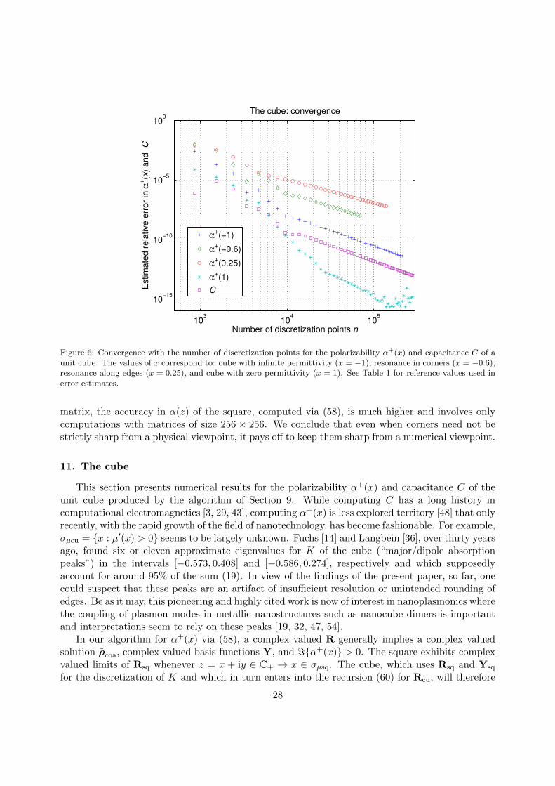
Figure 6: Convergence with the number of discretization points for the polarizability α+(x) and capacitance C of aunit cube. The values of x correspond to: cube with infinite permittivity (x = −1), resonance in corners (x = −0.6),resonance along edges (x = 0.25), and cube with zero permittivity (x = 1). See Table 1 for reference values used inerror estimates.

matrix, the accuracy in α(z) of the square, computed via (58), is much higher and involves onlycomputations with matrices of size 256 × 256. We conclude that even when corners need not bestrictly sharp from a physical viewpoint, it pays off to keep them sharp from a numerical viewpoint.

11. The cube

This section presents numerical results for the polarizability α+(x) and capacitance C of theunit cube produced by the algorithm of Section 9. While computing C has a long history incomputational electromagnetics [3, 29, 43], computing α+(x) is less explored territory [48] that onlyrecently, with the rapid growth of the field of nanotechnology, has become fashionable. For example,σµcu = {x : µ′(x) > 0} seems to be largely unknown. Fuchs [14] and Langbein [36], over thirty yearsago, found six or eleven approximate eigenvalues for K of the cube (“major/dipole absorptionpeaks”) in the intervals [−0.573, 0.408] and [−0.586, 0.274], respectively and which supposedlyaccount for around 95% of the sum (19). In view of the findings of the present paper, so far, onecould suspect that these peaks are an artifact of insufficient resolution or unintended rounding ofedges. Be as it may, this pioneering and highly cited work is now of interest in nanoplasmonics wherethe coupling of plasmon modes in metallic nanostructures such as nanocube dimers is importantand interpretations seem to rely on these peaks [19, 32, 47, 54].

In our algorithm for α+(x) via (58), a complex valued R generally implies a complex valuedsolution ρcoa, complex valued basis functions Y, and ={α+(x)} > 0. The square exhibits complexvalued limits of Rsq whenever z = x + iy ∈ C+ → x ∈ σµsq. The cube, which uses Rsq and Ysq

for the discretization of K and which in turn enters into the recursion (60) for Rcu, will therefore

28

have complex valued limits of Rcu and ={α+(x)} > 0 whenever x ∈ σµsq. We refer to this asresonance along edges. The reason being that ={α+(x)} > 0 implies x ∈ Spec(K,H−1/2) and, asa consequence of the symmetrization arguments in Section 5 and the fact that the spectrum of aself-adjoint operator consists of eigenvalues and approximate eigenvalues, each such x is either aneigenvalue or an approximate eigenvalue of K on H−1/2(S). Moreover, Rcu may remain complexvalued throughout the numerical homotopy process as z = x + iy ∈ C+ → x for other x ∈ [−1, 1]as well, that is, where limits of Rsq are real valued. We refer to this as resonance in corners.

Fig. 6 shows results from convergence tests. The total number of discretization points on thecube surface is n. The examples with n & 2 · 104 were executed on a workstation equipped withan IntelXeon E5430 CPU at 2.66 GHz and 32 GB of memory. Out of the chosen values of x, onecan see that the error in α+(x) is largest for x = 0.25. This is not surprising. A weakness inour algorithm is the assumption that the columns of Ysq are efficient basis functions for ρ(r) inthe direction perpendicular to an edge. When x = 0.25, there is resonance along edges and theshortcomings of this assumption should be particularly visible. When x = −1, x = 1 and for Cthere are real valued solutions ρ(r) ∈ L2(S) which are easier to resolve.

Table 1: Reference values, estimated relative errors, and best previous estimates for the limit polarizability α+(x)and the capacitance C of the cube.

present reference values relerr previous results Ref. relerr

α+(−1) 3.644305190268 10−11 3.6442 [48] 3 · 10−5

α+(−0.6) 5.85574775 + 16.64205643i 10−8

α+(0.25) −2.76289925 + 3.08034035i 10−7

α+(1) −1.638415712936517 10−14 −1.6383 [48] 6 · 10−5

C 0.66067815409957 10−13 0.66067813 [29] 10−7

The recursion (60) for Rcu requires a substantial amount of memory when np is large andNewton’s method is activated. This explains why the test series for α+(−0.6) in Fig. 6 had to beinterrupted at n = 69984, that is, for np = 27. Timings vary greatly with x, np, and the errortolerances that are set in recursions and iterative solvers. For safety, we set tolerances low andquote the following approximate computing times for n = 9600: α+(−1), α+(1), and C took oneminute each; α+(0.25) took two minutes; α+(−0.6) took ten minutes. The test series for α+(−1),α+(1) and C all confirm previous available results, see Table 1, and improve on these with betweensix and nine digits.

Fig. 7 is our main numerical result. It shows that the isolated cube has no bright plasmons (nopoles in α+(x)). For validation, see the figure caption, we have used the two sum rules (22), (23)and a third sum rule ∫

Rx2µ′(x) dx = 0.433464767896 , (66)

which has been determined numerically for the cube [22]. Fig. 7 also shows that σµcu is approx-imately equal to the interval (−0.694526, 0.5), possibly punctured at {−0.5, 0}, and raises theintriguing question of what surface shapes S lead to connected σµ. Our computed σµcu is broaderthan those estimated by earlier investigators [14, 32, 36] using other techniques. We conclude,again, that working with sharp edges and corners is an advantage.

29

−1 −0.5 0 0.5 1

−10

−5

0

5

10

15

20

The cube: polarizability

x

α+(x

)

real{α+(x)}

imag{α+(x)}

Figure 7: Polarizability of a cube. The curves are supported by 1195 data points whose relative accuracies rangefrom ten to five digits. No convergent results were obtained for α+(x) within a distance of 10−10 from x = −0.5 andwithin a distance of 10−5 from x = 0. The maximum value of <{α+(x)} is 20.00826 and occurs at x ≈ −0.694526.The sum rules (22), (23), and (66), evaluated via (25) using a composite trapezoidal rule, hold to a relative precisionof 3 · 10−5, 4 · 10−5, and 6 · 10−5, respectively.

12. Conclusions and outlook

We have constructed an electrostatic solver for cube-shaped domains and used it to producenew results for some canonical problems. A particular characteristic of the solver is that it takesadvantage of sharp edges and corners, rather than being a victim of them.

A mathematical framework capturing the symmetric features of the double layer potential andits adjoint has been identified, allowing for analysis of the polarizability α(z) through spectraltheory for self-adjoint operators. Moreover, this framework and its corresponding machinery isnatural and satisfactory also from a physical viewpoint, as the potentials produced to solve theelectrostatic problem are exactly those of finite energy. With full mathematical rigor we have shownhow to, with respect to polarizabilities, interpret the limit process which occurs when deforming asmooth surface into a cube, a point which has generated a fair amount of discussion in the materialsscience community.

Furthermore, we have shown that while the polarizability via limits can be extended to afunction α+(x) defined almost everywhere on the real axis, the same statement fails for the cor-responding potentials whenever the representing measure µ has a non-zero absolutely continuouspart. That is, no finite energy potential can be associated with a point x ∈ R where µ′(x) > 0 existsand is non-zero, neither as a direct solution to the electrostatic problem, nor as a limit from theupper half-plane. We remark, however, that while the density distributions ρx hence fail to existfor such x, the whole map x 7→ ρx can still be interpreted naturally as a vector-valued distribution.

For the cube, the mathematical theory in conjunction with the numerical findings show that

30

dµ(x) = µ′(x) dx is purely absolutely continuous, and that the set where µ′(x) > 0 is given by theinterval (a, b) ≈ (−0.694526, 0.5), possibly excepting the two points x = −0.5 and x = 0. Hence theintegral representation (44) for α(z), in terms of µ′(x), holds. Finally, µ′(x) has been determinednumerically. These discoveries, we hope, will be of use in plasmonics where absorption peaks ofnanocubes play an important role.

Future efforts will be directed towards solving the Helmholtz equation, compare [4, 5, 6]. Shouldthe polarizability of clusters of cubes or the effective permittivity of cubes in periodic arrangementsbe of interest, our solver requires only minor modifications.

Acknowledgements

We thank professors Alexandru Aleman, Anders Karlsson, Mihai Putinar, Daniel Sjoberg, andLaurian Suciu for useful conversations. This work was supported by the Swedish Research Councilunder contract 621-2011-5516.

References

[1] R. A. Adams, Sobolev spaces, Pure and Applied Mathematics, vol. 65, Academic Press, New York-London,1975.

[2] D. Bergman, The dielectric constant of a simple cubic array of identical spheres, J. Phys. C: Solid State Phys.12 (1979) 4947–4960.

[3] Y.I. Bontzios, M.G. Dimopoulos, and A.A. Hatzopulos, An evolutionary method for efficient computation ofmutual capacitance for VLSI circuits based on the method of images, Simul. Model. Pract. Th. 19 (2011)638–648.

[4] J. Bremer, A fast direct solver for the integral equations of scattering theory on planar curves with corners, J.Comput. Phys. 231 (2012) 1879–1899.

[5] J. Bremer, On the Nystrom discretization of integral equations on planar curves with corners, Appl. Comput.Harmon. Anal. 32 (2012) 45–64.

[6] J. Bremer, V. Rokhlin, and I. Sammis, Universal quadratures for boundary integral equations on two-dimensionaldomains with corners, J. Comput. Phys. 229 (2010) 8259–8280.

[7] O.P. Bruno, J.S. Oval, and C. Turc, A high-order integral algorithm for highly singular PDE solutions inLipschitz domains, Computing 84 (2009) 149–181.

[8] J. A. Cima, A. L. Matheson, W. T., The Cauchy transform, Mathematical Surveys and Monographs, vol. 125,American Mathematical Society, Providence, RI, 2006.

[9] R. R. Coifman, A. McIntosh, Y. Meyer, L’integrale de Cauchy definit un operateur borne sur L2 pour les courbeslipschitziennes, Ann. of Math. (2) 116 (1982) 361–387.

[10] R.V. Craster and Yu.V. Obnosov, Four-Phase Checkerboard Composites, SIAM J. Appl. Math. 61 (2001) 1839–1856.

[11] L. Escauriaza, E. B. Fabes, G. Verchota, On a regularity theorem for weak solutions to transmission problemswith internal Lipschitz boundaries, Proc. Amer. Math. Soc. 115 (1992) 1069–1076.

[12] E. Fabes, O. Mendez, M. Mitrea, Boundary layers on Sobolev-Besov spaces and Poisson’s equation for theLaplacian in Lipschitz domains, J. Funct. Anal. 159 (1998) 323–368.

[13] E. Fabes, M. Sand, J. K. Seo, The spectral radius of the classical layer potentials on convex domains, Partialdifferential equations with minimal smoothness and applications (Chicago, IL, 1990), 129–137, IMA Vol. Math.Appl., vol. 42, Springer, New York, 1992.

[14] R. Fuchs, Theory of the optical properties of ionic crystal cubes, Phys. Rev. B 11 (1975) 1732–1739.[15] R. Fuchs and S. H. Liu, Sum rule for the polarizability of small particles, Phys. Rev. B 14 (1976) 5521–5522.[16] E. Gagliardo, Caratterizzazioni delle tracce sulla frontiera relative ad alcune classi di funzioni in n variabili,

Rend. Sem. Mat. Univ. Padova 27 (1957) 284–305.[17] G. Geymonat, Trace theorems for Sobolev spaces on Lipschitz domains. Necessary conditions, Ann. Math. Blaise

Pascal 14 (2007) 187–197.[18] K. Golden and G. Papanicolaou, Bounds for effective parameters of heterogeneous media by analytic continua-

tion, Comm. Math. Phys. 90 (1983) 473–491.

31

[19] N. Grillet, D. Manchon, F. Bertorelle et al., Plasmon Coupling in Silver Nanocube Dimers: Resonance SplittingInduced by Edge Rounding, ACS NANO 5 (2011) 9450–9462.

[20] P. Grisvard, Elliptic problems in nonsmooth domains, Monographs and Studies in Mathematics, vol. 24, Pitman(Advanced Publishing Program), Boston, MA, 1985.

[21] S. Hassi, Z. Sebestyen, H. S. V. de Snoo, On the nonnegativity of operator products, Acta Math. Hungar. 109(2005) 1–14.

[22] J. Helsing, Third-order bounds on the conductivity of a random stacking of cubes, J. Math. Phys. 35 (1991)1688–1692.

[23] J. Helsing, Integral equation methods for elliptic problems with boundary conditions of mixed type, J. Comput.Phys. 228 (2009) 8892–8907.

[24] J. Helsing, A fast and stable solver for singular integral equations on piecewise smooth curves, SIAM J. Sci.Comput. 33 (2011) 153–174.

[25] J. Helsing, The effective conductivity of arrays of squares: large random unit cells and extreme contrast ratios,J. Comput. Phys. 230 (2011) 7533–7547.

[26] J. Helsing and R. Ojala, Corner singularities for elliptic problems: Integral equations, graded meshes, quadrature,and compressed inverse preconditioning, J. Comput. Phys. 227 (2008) 8820–8840.

[27] J. Helsing and R. Ojala, Elastostatic computations on aggregates of grains with sharp interfaces, corners, andtriple-junctions, Int. J. Solids Struct. 46 (2009) 4437–4450.

[28] S. Hofmann, M. Mitrea, M. Taylor, Singular integrals and elliptic boundary problems on regular Semmes-Kenig-Toro domains, Int. Math. Res. Not. 2010, no. 14, 2567–2865.

[29] C.-O. Hwang, M. Mascagni, and T. Won, Monte Carlo methods for computing the capacitance of the unit cube,Math. Comput. Simulat. 80 (2010) 1089–1095.

[30] H. Kettunen, H. Wallen, and A. Sihvola, Electrostatic resonances of negative-permittivity hemisphere, J. Appl.Phys. 103 (2008) 094112.

[31] D. Khavinson, M. Putinar, H. S. Shapiro, Poincare’s variational problem in potential theory, Arch. Ration.Mech. Anal. 185 (2007) 143–184.

[32] V.V. Klimov, Ya.N. Istomin, and Yu.A. Kosevich, Plasma phenomena in nanostructures and neutron stars,Physics–Uspekhi 51 (2008) 839–859.

[33] P. Koosis, Introduction to Hp spaces, Second edition, With two appendices by V. P. Havin, Cambridge Tractsin Mathematics, vol. 115, Cambridge University Press, Cambridge, 1998.

[34] M. G. Krein, Compact linear operators on functional spaces with two norms, Dedicated to the memory of MarkGrigorievich Krein (1907–1989), Integral Equations Operator Theory 30 (1998) 140–162.

[35] R. Kuhnau, Moglichst konforme Spiegelung an einer Jordankurve, Jahresber. Deutsch. Math.-Verein. 90 (1988)90–109.

[36] D. Langbein, Normal modes at small cubes and rectangular particles, J. Phys. A: Math. Gen. 9 (1976) 627–644.[37] I.D. Mayergoyz, D. R. Fredkin, and Z. Zhang, Electrostatic (plasmon) resonances in nanoparticles, Phys. Rev.

B 72 (2005) 155412.[38] Y. Meyer, Ondelettes et operateurs. II., Operateurs de Calderon-Zygmund. Actualites Mathematiques, Hermann,

Paris, 1990.[39] G.W. Milton, R.C. McPhedran, and D.R. McKenzie, Transport properties of arrays of intersecting cylinders,

Appl. Phys. 25 (1981) 23–30.[40] G.W. Milton, Proof of a conjecture on the conductivity of checkerboards, J. Math. Phys. 42 (2001) 4873–4882.[41] D. Mitrea, The method of layer potentials for non-smooth domains with arbitrary topology, Integral Equations

Operator Theory 29 (1997) 320–338.[42] I. Mitrea, On the spectra of elastostatic and hydrostatic layer potentials on curvilinear polygons, J. Fourier

Anal. Appl. 8 (2002) 443–487.[43] S. Mukhopadhyay and N. Majumdar, A study of three-dimensional edge and corner problems using the neBEM

solver, Eng. Anal. Bound. Elem. 33 (2009) 105–119.[44] W.T. Perrins and R.C. McPhedran, Metamaterials and the homogenization of composite materials, Metamate-

rials 4 (2010) 24–31.[45] M. Pitkonen, A closed-form solution for the polarizability of a dielectric double half-cylinder, J. Electromagnet.

Wave. 24 (2010) 1267–1277.[46] F.H. Read, Capacitances and singularities of the unit triangle, square, tetrahedron and cube, COMPEL 23

(2004) 572–578.[47] R. Ruppin, Plasmon frequences of cube shaped metal clusters, Z. Phys. D. 36 (1996) 69–71.[48] A. Sihvola, P. Yla-Oijala, S. Jarvenpaa, and J. Avelin, Polarizabilities of Platonic Solids, IEEE Trans. Antennas

32

Propagat. 52 (2004) 2226–2233.[49] M.F. Thorpe, The conductivity of a sheet containing a few polygonal holes and/or superconducting inclusions,

Proc. R. Soc. Lond. A 437 (1992) 215–227.[50] G. Verchota, Layer potentials and regularity for the Dirichlet problem for Laplace’s equation in Lipschitz

domains, J. Funct. Anal. 59 (1984) 572–611.[51] H. Wallen, H. Kettunen, and A. Sihvola, Surface modes of negative-parameter interfaces and the importance of

rounding sharp corners, Metamaterials 2 (2008) 113–121.[52] J. Weidmann, Strong operator convergence and spectral theory of ordinary differential operators, Univ. Iagel.

Acta Math. 34 (1997) 153–163.[53] S. Werner, Spiegelungskoeffizient und Fredholmscher Eigenwert fur gewisse Polygone, Ann. Acad. Sci. Fenn.

Math. 22 (1997) 165–186.[54] S. Zhang, K. Bao, N.J. Halas, H. Xu, and P. Nordlander, Substrate-Induced Fano Resonances of a Plasmonic

Nanocube: A Route to Increased-Sensitivity Localized Surface Plasmon Resonance Sensors Revealed, NanoLett. 11 (2011) 1657–1663.

33