THE JOURNAL OF CHEMICAL PHYSICS 135, 134105 (2011)

Polarizability and alignment of dielectric nanoparticles in an externalelectric field: Bowls, dumbbells, and cuboids

Bas W. Kwaadgras,1,a) Maarten Verdult,2 Marjolein Dijkstra,1 and René van Roij21Soft Condensed Matter, Debye Institute for Nanomaterials Science, Utrecht University, Princetonplein 5,3584 CC Utrecht, the Netherlands2Institute for Theoretical Physics, Utrecht University, Leuvenlaan 4, 3584 CE Utrecht, the Netherlands

(Received 18 May 2011; accepted 19 August 2011; published online 3 October 2011)

We employ the coupled dipole method to calculate the polarizability tensor of various anisotropicdielectric clusters of polarizable atoms, such as cuboid-, bowl-, and dumbbell-shaped nanoparticles.Starting from a Hamiltonian of a many-atom system, we investigate how this tensor depends onthe size and shape of the cluster. We use the polarizability tensor to calculate the energy differenceassociated with turning a nanocluster from its least to its most favorable orientation in a homogeneousstatic electric field, and we determine the cluster dimension for which this energy difference exceedsthe thermal energy such that particle alignment by the field is possible. Finally, we study in detail the(local) polarizability of a cubic-shaped cluster and present results indicating that, when retardation isignored, a bulk polarizability cannot be reached by scaling up the system. © 2011 American Instituteof Physics. [doi:10.1063/1.3637046]

I. INTRODUCTION

Monodisperse (colloidal) particles with a wide variety ofshapes can nowadays be synthesized in the nanometer to mi-crometer size regime.1, 2 These particles can serve as buildingblocks for new materials and devices with great technolog-ical potential. Self-assembly of the particles is an importantprocess by which large-scale nano-structures can be formed.This self-assembly process can be spontaneous in the caseof favorable thermodynamic conditions and suitable effec-tive particle-particle interactions,3–10 but can also be steeredand further manipulated by external fields. Rodlike parti-cles in a liquid dispersion, for instance, can spontaneouslyalign at sufficiently high concentrations solely due to their ex-cluded volume interactions,11 but their self-organisation hasalso been driven by external magnetic or electric fields,12–16

by substrates that preferentially orient the rods,17, 18 or byfluid flow.19 Also, more complicated shapes have been syn-thesized and studied, for instance, dumbbells,2, 20–22 cubes,23

and bowls.21, 24, 25

In this article we study the electric-field assisted align-ment of anisotropic nanoparticles by calculating their polar-izability tensor starting from a microscopic picture of po-larizable units that we call “united atoms” or just briefly“atoms,” even though also larger units could have been taken.We only consider dielectric particles,26, 27 and not metal-lic particles.28–30 From the polarizability tensor of a non-spherical cluster of atoms, the orientation-dependent electro-static energy follows, and hence the cluster’s ability to alignin an external electric field. We focus here on cuboid-shaped(rods and platelets), bowl-shaped, and dumbbell-shaped par-ticles, for which we consider various shape and size parame-ters. The polarizability of similar shapes have in recent years

a)Author to whom correspondence should be addressed. Electronic mail:b.w.kwaadgras@uu.nl.

been under study using continuum theory31–35 and on severaloccasions we briefly compare those results to ours.

Our calculations are based on the coupled dipole method(CDM), a formalism introduced by Renne and Nijboer in the1960s.36, 37 In the CDM, each atom in a cluster is treated asa Lorentz atom (or Drude oscillator), in which the electron isbound to the nucleus by a harmonic force. The atoms haveno permanent electric dipole moment, but their dipole mo-ments are induced by the local electric field. This model hasbeen shown to yield the van der Waals interaction betweentwo atoms.36, 38, 39 In the CDM, many such dipolar atoms in-teract and the potential energy, including all many-body ef-fects, can be calculated from the eigenfrequencies of a setof coupled harmonic oscillators, yielding forces equivalent toLifschitz’s quantum-electrodynamic fluctuation theory.40 Dueto its full many-body nature the CDM is more accurate thancontinuum theories based on pairwise summations of atomicvan der Waals interactions, as employed in, e.g., the Hamaker-de Boer approach41, 42 that underlies the treatment of disper-sion forces in DLVO-theory.43, 44 In this article we do not con-sider solvent effects explicitly.

II. FORMALISM OF THE CDM: POTENTIAL ENERGY,POLARIZABILITY, AND ORIENTATIONAL ENERGY

A. Introduction

In the Lorentz model for atoms in an external electricfield, an atom is modeled as a dipole consisting of a nucleusand an electron bound to it by a harmonic force. Thus, if theelectron is at a nonzero distance from the nucleus, the atomis effectively an induced electric dipole. In this simple model,the displacement u of the electron with respect to the nucleus,and thus the atom’s polarization p = eu, is linearly dependent

0021-9606/2011/135(13)/134105/15/$30.00 © 2011 American Institute of Physics135, 134105-1

Author complimentary copy. Redistribution subject to AIP license or copyright, see http://jcp.aip.org/jcp/copyright.jsp

134105-2 Kwaadgras et al. J. Chem. Phys. 135, 134105 (2011)

on the local electric field E that the atom is subjected to,

eu = p = α0E,

where e is the elementary charge. Here, α0 is the polarizabilityof the atom, given by

α0 = e2

meω20

, (1)

where me denotes the electron mass and ω0 is the angular fre-quency associated with the harmonic force that binds the elec-tron to the nucleus.45 Since an electric dipole will produce anonzero electric field in its surroundings, two of these Lorentzatoms will interact, mediated by the electric field. It has beenshown that this dipole-dipole interaction yields the unretardedVan der Waals interaction (∝ r−6) between the pair of atoms(at large separation r).36 If N of these atoms are brought to-gether and allowed to interact, the dipole-dipole interactionswill influence the electric properties of the cluster as a whole.In general, the total polarizability of the cluster cannot be ex-pected to equal Nα0, but will instead be modified because theatoms are subject to each other’s induced electric field.

B. Static polarizability and orientational energy ofdipole clusters in an external electric field

The Hamiltonian of a set of N Lorentz atoms at fixedpositions ri (i = 1, . . . , N) has been given and studied inRefs. 27, 36, 38, 46–48. In the present work, we use the sameHamiltonian, but add an extra term to allow for an externallyexerted, spatially homogeneous, electric field E0, such that thecomplete expression for the Hamiltonian is

H =N∑

i=1

k2i

2me

+N∑

i=1

meω20u2

i

2

−N∑

i,j=1

e2ui · Tij · uj

2−

N∑i=1

eui · E0, (2)

where we denote the momentum of the electron of atom i byki . The 3 × 3 matrix Tij is the dipolar tensor, given in termsof the separation vector rij = ri − rj of atoms i and j , by

Tij =⎧⎨⎩

(3rij rij /|rij |2 − I)

|rij |3 , if i �= j

0, if i = j

,

where I denotes the 3 × 3 identity matrix and 0 denotes the3 × 3 null matrix. Note that the dipolar tensor is not onlysymmetric in its indices, Tij = Tji , but also symmetric in itselements, Tij = TT

ij . As is clear from the Hamiltonian equa-tion (2) and the form of Tij , this model describes interatomicinteractions in an instantaneous, nonretarded way. Therefore,the validity of the theory is limited to model systems wherethe relevant length scales are small enough for the speed oflight to be essentially infinite.

We now introduce 3N -dimensional vectors K, U , and E0,which are built up from the ki , ui , and N copies of E0, re-

spectively. We also introduce a 3N × 3N -dimensional matrixT , built up from the Tij . In terms of these objects, the Hamil-tonian equation (2) is given by

H = K2

2me

+ 1

2meω

20U · (I − α0T ) · U − eU · E0,

where α0 is given in Eq. (1), and I denotes the 3N

× 3N -dimensional identity matrix. Next, we introduce a3N -dimensional vector U0 that satisfies

meω20 (I − α0T ) · U0 = eE0, (3)

and use it to complete the square in the Hamiltonian,obtaining

H = H0 + VE (4)

with

H0 = K2

2me

+ 1

2meω

20(U − U0) · (I − α0T ) · (U − U0),

(5)

VE = −1

2α0E0 · (I − α0T )−1 · E0. (6)

Note that VE is constant with respect to the generalized mo-menta and coordinates K and U − U0, respectively. The 3N

oscillatory modes associated with the (harmonic) Hamilto-nian H0 are given by

(U (k) − U0) (t) = (U (k) − U0) (0) exp (−iωkt) ,

(k = 1, . . . , 3N ), (7)

where the amplitude vectors (U (k) − U0)(0) and the frequen-cies ωk are given by an eigenvalue equation for the matrix(I − α0T ):

ω2k

ω20

(U (k) − U0) (0) = (I − α0T ) (U (k) − U0) (0) . (8)

If we denote the eigenvalues of the matrix T by λk , it is seenthat the eigenvalues of (I − α0T ) are (1 − α0λk), and thusthat the allowed frequencies are

ωk = ω0

√1 − α0λk.

Assuming the system to be in the electronic ground state, wearrive at the total potential energy

V = V0 + VE, (9)

where V0 is the ground state energy of H0, given by the sumof mode frequencies,

V0 = 1

2¯

3N∑k=1

ωk, (10)

where ¯ is the reduced Planck constant.We note that V0 depends solely on the matrix (I − α0T )

and, thus, only on the relative coordinates rij of the atomswith respect to each other. It follows that this term is com-pletely independent of the orientation of the cluster with re-spect to the electric field. In the absence of other clusters, V0

can therefore be interpreted as the self-energy of the cluster;

Author complimentary copy. Redistribution subject to AIP license or copyright, see http://jcp.aip.org/jcp/copyright.jsp

134105-3 Polarizability and alignment of nanoparticles J. Chem. Phys. 135, 134105 (2011)

in the presence of other clusters, the term also contains the in-teraction energy between the clusters.46 For the analysis of theresponse of the clusters to an external electric field, however,we turn to the second term VE of Eq. (9): this term, given inEq. (6), contains all the orientational potential energy of thecluster in the external electric field.

Clearly, the Hamiltonian of Eq. (4) describes a set of har-monic oscillators with equilibrium positions given by U0 anda shifted ground state energy V . Using this interpretation ofU0, we show, in the following, that VE is the energy of thetotal time-averaged dipole moment of the cluster in the exter-nal electric field. We first rewrite Eq. (3) in terms of the meanpolarization vector P ≡ eU0,

(I − α0T ) · P = α0E0, (11)

and use this equation, in combination with the expression forVE given in Eq. (6), to derive

VE = −1

2E0 · P = −1

2E0 · pc, (12)

where

pc ≡N∑

i=1

pi (13)

denotes the total polarization of the cluster and pi ≡ eu0,i

denotes the mean (time-averaged) polarization of atom i, asgiven by the elements of P . From the form of Eq. (12), itis clear that VE is the energy of an induced dipole pc in anelectric field E0.45 If we divide the matrix (I − α0T )−1 into3 × 3 sub-blocks Dij , it can easily be seen from Eq. (11) thatpi = α0

∑j Dij · E0, and thus that

pc = α0

N∑i,j=1

Dij · E0 ≡ αc · E0, (14)

where we define the 3 × 3 cluster polarizability matrix by

αc ≡ α0

N∑i,j=1

Dij . (15)

An alternative derivation of Eqs. (11)–(14) is given inRef. 26. Note that αc depends solely on the spatial configu-rational properties of the cluster, not on the external electricfield. Moreover, one can prove mathematically that αc is asymmetric matrix, as long as each atom has an equal polariz-ability α0.49 This symmetry of αc implies that its eigenvectorsare orthogonal, which in turn implies that it is always possi-ble to transform the system to an orthogonal basis, spannedby these eigenvectors, in which αc is diagonal.

Computationally, Eq. (15) is not a practical way of de-termining αc, since it involves the very expensive operationof explicitly calculating the inverse of a large matrix. Numer-ically, the most favorable approach is to use Eq. (14): afterchoosing a suitable coordinate system, we apply an electricfield in the x direction and calculate the cluster polarizationby solving Eq. (11). Efficient numerical algorithms for solv-ing a set of linear equations are readily available, for example,in the LAPACK package.50 Having solved Eq. (11) for P , wecalculate the sum in Eq. (13), then divide the resulting vector

by the electric field strength; the result is the first column ofαc. To gain the remaining two columns, this procedure is thenrepeated in the other two Cartesian directions.

If we were to neglect the dipolar interactions within thecluster, its polarization would be simply Nα0E0, i.e., the clus-ter polarizability would simply be a scalar Nα0. The ratio ofthe “actual” polarizability αc and this “naive” guess for thepolarizability,

f = αc

Nα0, (16)

is a measure of how much the polarizability is enhanced dueto dipole-dipole interactions and may therefore be called the“enhancement factor” of the dipole cluster.26

In terms of αc, we can rewrite Eq. (12) compactly as

VE = −1

2E0 · αc · E0. (17)

This expression can then be written in terms of the eigen-values αn and the corresponding normalized eigenvectors vn

(n = 1, 2, 3) of αc:

VE = −1

2

3∑n,m=1

(E0 · vn) (vn · αc · vm) (vm · E0)

= −1

2

3∑n=1

(E0 · vn)2 αn. (18)

In the first line, we inserted twice a complete orthonormal setof eigenvectors, while, in the second line, we made use of thefact that αc · vm = αmvm and vn · vm = δnm. The inner prod-ucts obey the rule

∑n (E0 · vn)2 = E2

0 , from which it followsthat

∑3n=1 (E0 · vn)2 αn ≤ αmaxE

20 , where αmax = max ({αn})

and the equality is achieved if and only if E0 ‖ vmax , wherevmax is the eigenvector corresponding to αmax . It follows thatVE is minimized by an electric field in the direction of vmax .A similar reasoning leads to the observation that VE is max-imized by an electric field in the direction of the eigenvec-tor with the smallest eigenvalue, αmin. The difference |�|between maximum and minimum orientational energy VE isthus given by

|�| = 1

2(αmax − αmin) E2

0 .

Here, for later purposes, we intentionally kept the freedom ofchoosing the sign of �.

C. Rotationally symmetric clusters

The bowl- and dumbbell-shaped nanoparticles consid-ered in this article are clusters with an axis of rotational sym-metry. The rotational invariance implies that the polarizationthat would be induced by an electric field in the direction ofthe symmetry axis must lie along this symmetry axis, andtherefore that this axis is an eigenvector of the cluster’s po-larizability matrix αc. Since it is known that αc must be asymmetric matrix, we know that its eigenvectors must be per-pendicular to each other. This leads to the conclusion that thepreferred direction of any rotationally symmetric cluster musteither lie along the rotational symmetry axis or perpendicular

Author complimentary copy. Redistribution subject to AIP license or copyright, see http://jcp.aip.org/jcp/copyright.jsp

134105-4 Kwaadgras et al. J. Chem. Phys. 135, 134105 (2011)

to it. In this article, we always choose our coordinate systemsuch that this rotational symmetry axis lies along the z axis,and choose the x and y directions such that αc is diagonal(i.e., the Cartesian axes are the eigenvectors of αc). Moreover,for rotationally symmetric clusters, αxx = αyy , and hence weare left with only two independent entries on the diagonal ofαc, one of which will be αmax and the other will be αmin. Forthe remainder of this article, we now define the orientationalenergy difference as51

� ≡ 1

2(αzz − αxx) E2

0 , (19)

where we choose the sign of � such that � is positive whenthe preferred direction of the cluster is along the rotationalsymmetry axis (which is equivalent to αzz > αxx).

Using Eq. (16), we can write Eq. (19) as

� = 1

2�f Nα0E

20 , (20)

where

�f = fzz − fxx.

As will be shown for all the cluster shapes in this article, thequantity �f is largely independent of the cluster size, pro-vided the number of atoms is large enough. In this regime,�f depends only on the shape of the cluster and on the di-mensionless interatomic distance a/α

1/30 . This assertion does

not state anything about the individual values of fzz and fxx

as a function of cluster size. From the numerical data, it turnsout that these quantities can still depend on cluster size, albeitusually only weakly.

It is of interest to compare � to the thermal energy kBT ,since only if � � kBT , an electric field can be used to orientthe particle. Equating � = kBT we derive the required num-ber of atoms N∗ from Eq. (20),

N∗ = 2kBT

�f α0E20

. (21)

In Sec. IV, we will use this expression to calculate N∗ forbowls and dumbbells and hence estimate the spatial dimen-sions required for aligning these particles using an electricfield.

D. Fourfold rotationally symmetric clusters

One of the discussed cluster shapes in this article is acluster with a cubic shape. If we choose the coordinate axesalong the ribs of the cube, it can be easily seen from sym-metry considerations that an electric field applied in the x di-rection must induce a total cluster polarization p(cube)

c with anonzero component only in the x direction. Similarly, the po-larizations as a result of electric fields in the y and z directionswill also point along the y and z axes, respectively. Becausethese resulting polarizations are proportional to the columnsof α(cube)

c , it follows that α(cube)c must be diagonal in this basis.

Moreover, because the cube is invariant under 90◦ rotations,we do not expect the induced polarization of the cube to bedependent on whether the electric field is applied in the x, y,or z direction and, therefore, the entries on the diagonal of

α(cube)c must be equal. Hence,

α(cube)c ∝ I. (22)

Note that, in this case, both the polarizability and the en-hancement factor can be described by a scalar: the former bythe proportionality factor between α(cube)

c and I, the latter bythis “scalar polarizability” divided by Nα0. Since in this caseαxx = αyy = αzz, we find, from Eq. (19), that � = 0. Thiskind of cluster will therefore not have a preferred orientationwithin an external electric field. Physically, this is a surprisingresult since, a priori, one could expect an anisotropic clustersuch as a cube to prefer to align one of its features (such as itsribs, faces, or vertices) along the electric field. However, sim-ple symmetry arguments negate this expectation. For cuboid-shaped rods and platelets, on the other hand, as is the casefor bowls and dumbbells, αxx = αyy �= αzz and hence � �= 0.In Sec. III, we will use Eq. (21) to calculate N∗ for rods andplatelets and estimate the minimum size of the particles toalign them in an electric field.

E. Units of distance

Throughout the remainder of this paper, we will usuallymeasure lattice spacings in units of α

1/30 . The reason is that,

throughout the theory, the matrix T is always multiplied by afactor α0. Upon applying this multiplication to the submatri-ces Tij , we get

α0Tij = (3sij sij /|sij |2 − I)

|sij |3 (i �= j ) ,

where

sij = rij /α1/30 .

Clearly, the relevant parameters are not the rij themselves, butrather the dimensionless combinations sij = rij /α

1/30 . Using

these dimensionless distances, we thus eliminate the atomicpolarizability as an explicit input parameter. At the same time,the dimensionless combinations are O (1) in magnitude (fortypical lattices and atomic polarizabilities), which is conve-nient for computational purposes. We use the numerical dataprovided in Ref. 26 to calculate the dimensionless latticespacing

a ≡ a/α1/30

for several substances, the result of which is listed inTable I. For clarity, we note here that all other physical quan-tities remain unscaled in this paper.

TABLE I. Lattice spacings a, atomic polarizabilities α0, and dimensionlesslattice spacings a ≡ a/α

1/30 of some typical substances. (See Ref. 26.)

Substance a(Å) α0(Å3) a

Hexane 6.009 11.85 2.64Silica 3.569 5.25 2.05Sapphire 3.486 7.88 1.75

Author complimentary copy. Redistribution subject to AIP license or copyright, see http://jcp.aip.org/jcp/copyright.jsp

134105-5 Polarizability and alignment of nanoparticles J. Chem. Phys. 135, 134105 (2011)

III. DIELECTRIC RODS AND PLATELETS

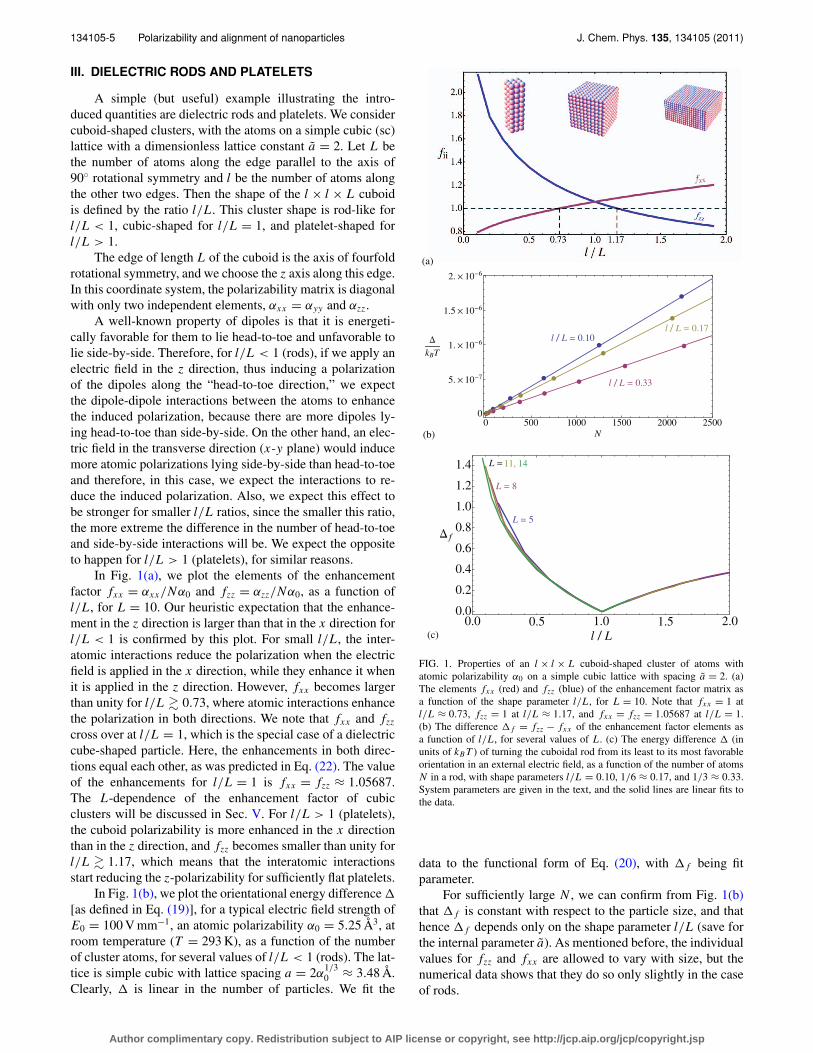
A simple (but useful) example illustrating the intro-duced quantities are dielectric rods and platelets. We considercuboid-shaped clusters, with the atoms on a simple cubic (sc)lattice with a dimensionless lattice constant a = 2. Let L bethe number of atoms along the edge parallel to the axis of90◦ rotational symmetry and l be the number of atoms alongthe other two edges. Then the shape of the l × l × L cuboidis defined by the ratio l/L. This cluster shape is rod-like forl/L < 1, cubic-shaped for l/L = 1, and platelet-shaped forl/L > 1.

The edge of length L of the cuboid is the axis of fourfoldrotational symmetry, and we choose the z axis along this edge.In this coordinate system, the polarizability matrix is diagonalwith only two independent elements, αxx = αyy and αzz.

A well-known property of dipoles is that it is energeti-cally favorable for them to lie head-to-toe and unfavorable tolie side-by-side. Therefore, for l/L < 1 (rods), if we apply anelectric field in the z direction, thus inducing a polarizationof the dipoles along the “head-to-toe direction,” we expectthe dipole-dipole interactions between the atoms to enhancethe induced polarization, because there are more dipoles ly-ing head-to-toe than side-by-side. On the other hand, an elec-tric field in the transverse direction (x-y plane) would inducemore atomic polarizations lying side-by-side than head-to-toeand therefore, in this case, we expect the interactions to re-duce the induced polarization. Also, we expect this effect tobe stronger for smaller l/L ratios, since the smaller this ratio,the more extreme the difference in the number of head-to-toeand side-by-side interactions will be. We expect the oppositeto happen for l/L > 1 (platelets), for similar reasons.

In Fig. 1(a), we plot the elements of the enhancementfactor fxx = αxx/Nα0 and fzz = αzz/Nα0, as a function ofl/L, for L = 10. Our heuristic expectation that the enhance-ment in the z direction is larger than that in the x direction forl/L < 1 is confirmed by this plot. For small l/L, the inter-atomic interactions reduce the polarization when the electricfield is applied in the x direction, while they enhance it whenit is applied in the z direction. However, fxx becomes largerthan unity for l/L � 0.73, where atomic interactions enhancethe polarization in both directions. We note that fxx and fzz

cross over at l/L = 1, which is the special case of a dielectriccube-shaped particle. Here, the enhancements in both direc-tions equal each other, as was predicted in Eq. (22). The valueof the enhancements for l/L = 1 is fxx = fzz ≈ 1.05687.The L-dependence of the enhancement factor of cubicclusters will be discussed in Sec. V. For l/L > 1 (platelets),the cuboid polarizability is more enhanced in the x directionthan in the z direction, and fzz becomes smaller than unity forl/L � 1.17, which means that the interatomic interactionsstart reducing the z-polarizability for sufficiently flat platelets.

In Fig. 1(b), we plot the orientational energy difference �

[as defined in Eq. (19)], for a typical electric field strength ofE0 = 100 V mm−1, an atomic polarizability α0 = 5.25 Å3, atroom temperature (T = 293 K), as a function of the numberof cluster atoms, for several values of l/L < 1 (rods). The lat-tice is simple cubic with lattice spacing a = 2α

1/30 ≈ 3.48 Å.

Clearly, � is linear in the number of particles. We fit the

l / L 0.10

l / L 0.33

l / L 0.17

0 500 1000 1500 2000 25000

5. 10 7

1. 10 6

1.5 10 6

2. 10 6

N

kBT

L 5

L 8

L 11, 14

0.0 0.5 1.0 1.5 2.00.0

0.2

0.4

0.6

0.8

1.0

1.2

1.4

l / L

f

(b)

(a)

(c)

FIG. 1. Properties of an l × l × L cuboid-shaped cluster of atoms withatomic polarizability α0 on a simple cubic lattice with spacing a = 2. (a)The elements fxx (red) and fzz (blue) of the enhancement factor matrix asa function of the shape parameter l/L, for L = 10. Note that fxx = 1 atl/L ≈ 0.73, fzz = 1 at l/L ≈ 1.17, and fxx = fzz = 1.05687 at l/L = 1.(b) The difference �f = fzz − fxx of the enhancement factor elements asa function of l/L, for several values of L. (c) The energy difference � (inunits of kBT ) of turning the cuboidal rod from its least to its most favorableorientation in an external electric field, as a function of the number of atomsN in a rod, with shape parameters l/L = 0.10, 1/6 ≈ 0.17, and 1/3 ≈ 0.33.System parameters are given in the text, and the solid lines are linear fits tothe data.

data to the functional form of Eq. (20), with �f being fitparameter.

For sufficiently large N , we can confirm from Fig. 1(b)that �f is constant with respect to the particle size, and thathence �f depends only on the shape parameter l/L (save forthe internal parameter a). As mentioned before, the individualvalues for fzz and fxx are allowed to vary with size, but thenumerical data shows that they do so only slightly in the caseof rods.

Author complimentary copy. Redistribution subject to AIP license or copyright, see http://jcp.aip.org/jcp/copyright.jsp

134105-6 Kwaadgras et al. J. Chem. Phys. 135, 134105 (2011)

As an example, for l/L = 0.10, we find, for the param-eters of Fig. 1(b), that �f ≈ 1.1. By substituting the afore-mentioned numerical data into Eq. (21), it follows that N∗

≈ 1.3 × 109. Using the shape parameter l/L = 0.1, the num-ber of atoms along the long edge of the cuboid is calculated asL∗ = (100N∗)1/3 ≈ 5.0 × 103 which, using a ≈ 3.48 Å, cor-responds to a physical length of the long edge of ∼1.8 μmand corresponding length of the short edges of 0.18 μm.

A simple order-of-magnitude calculation shows that re-tardation effects, which are not included in our theory, be-come important when length scales are of the order of∼500 nm. The estimate of 1.8 μm for alignment exceeds thislength scale and thus, retardation effects are expected to beimportant. The exact magnitude of the error this produces inour estimate is hard to determine without including retarda-tion effects in the CDM, but the expectation is that the errorwill be marginal, since our estimated length scale does notdramatically exceed the 500 nm boundary.

In Fig. 1(c), we plot �f as a function of l/L, for sev-eral values of L. Interestingly, these graphs overlap for suf-ficiently large N , again confirming the independence of �f

of L. It appears that for cuboids, a “sufficiently large N” iseasily achieved: already for l × l × 5 cuboids, there is almostperfect collapse of the data.

A. Dielectric strings

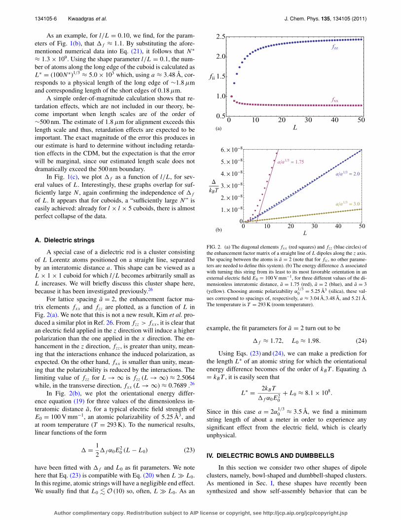
A special case of a dielectric rod is a cluster consistingof L Lorentz atoms positioned on a straight line, separatedby an interatomic distance a. This shape can be viewed as aL × 1 × 1 cuboid for which l/L becomes arbitrarily small asL increases. We will briefly discuss this cluster shape here,because it has been investigated previously.26

For lattice spacing a = 2, the enhancement factor ma-trix elements fxx and fzz are plotted, as a function of L inFig. 2(a). We note that this is not a new result, Kim et al. pro-duced a similar plot in Ref. 26. From fzz > fxx , it is clear thatan electric field applied in the z direction will induce a higherpolarization than the one applied in the x direction. The en-hancement in the z direction, fzz, is greater than unity, mean-ing that the interactions enhance the induced polarization, asexpected. On the other hand, fxx is smaller than unity, mean-ing that the polarizability is reduced by the interactions. Thelimiting value of fzz for L → ∞ is fzz (L → ∞) ≈ 2.5064while, in the transverse direction, fxx (L → ∞) ≈ 0.7689 .26

In Fig. 2(b), we plot the orientational energy differ-ence equation (19) for three values of the dimensionless in-teratomic distance a, for a typical electric field strength ofE0 = 100 V mm−1, an atomic polarizability of 5.25 Å3, andat room temperature (T = 293 K). To the numerical results,linear functions of the form

� = 1

2�f α0E

20 (L − L0) (23)

have been fitted with �f and L0 as fit parameters. We notehere that Eq. (23) is compatible with Eq. (20) when L L0.In this regime, atomic strings will have a negligible end effect.We usually find that L0 � O (10) so, often, L L0. As an

fzz

fxx

0 10 20 30 40 500.5

1.0

1.5

2.0

2.5

L

fii

a Α1 3 1.75

a Α1 3 2.0

a Α1 3 3.0

0 10 20 30 40 500

1. 10 8

2. 10 8

3. 10 8

4. 10 8

5. 10 8

6. 10 8

L

kBT

(a)

(b)

FIG. 2. (a) The diagonal elements fxx (red squares) and fzz (blue circles) ofthe enhancement factor matrix of a straight line of L dipoles along the z axis.The spacing between the atoms is a = 2 (note that for fii , no other parame-ters are needed to define this system). (b) The energy difference � associatedwith turning this string from its least to its most favorable orientation in anexternal electric field E0 = 100 V mm−1, for three different values of the di-mensionless interatomic distance, a = 1.75 (red), a = 2 (blue), and a = 3(yellow). Choosing atomic polarizability α

1/30 = 5.25 Å3 (silica), these val-

ues correspond to spacings of, respectively, a ≈ 3.04 Å,3.48 Å, and 5.21 Å.The temperature is T = 293 K (room temperature).

example, the fit parameters for a = 2 turn out to be

�f ≈ 1.72, L0 ≈ 1.98. (24)

Using Eqs. (23) and (24), we can make a prediction forthe length L∗ of an atomic string for which the orientationalenergy difference becomes of the order of kBT . Equating �

= kBT , it is easily seen that

L∗ = 2kBT

�f α0E20

+ L0 ≈ 8.1 × 108.

Since in this case a = 2α1/30 ≈ 3.5 Å, we find a minimum

string length of about a meter in order to experience anysignificant effect from the electric field, which is clearlyunphysical.

IV. DIELECTRIC BOWLS AND DUMBBELLS

In this section we consider two other shapes of dipoleclusters, namely, bowl-shaped and dumbbell-shaped clusters.As mentioned in Sec. I, these shapes have recently beensynthesized and show self-assembly behavior that can be

Author complimentary copy. Redistribution subject to AIP license or copyright, see http://jcp.aip.org/jcp/copyright.jsp

134105-7 Polarizability and alignment of nanoparticles J. Chem. Phys. 135, 134105 (2011)

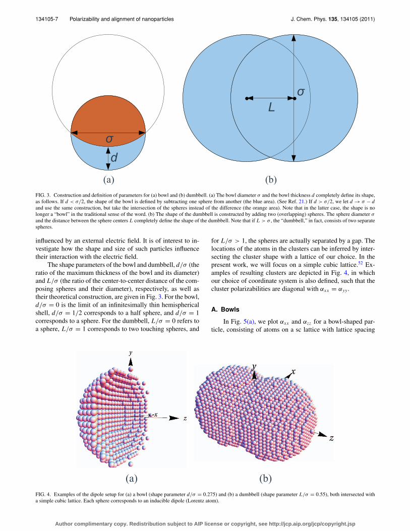
FIG. 3. Construction and definition of parameters for (a) bowl and (b) dumbbell. (a) The bowl diameter σ and the bowl thickness d completely define its shape,as follows. If d < σ/2, the shape of the bowl is defined by subtracting one sphere from another (the blue area). (See Ref. 21.) If d > σ/2, we let d → σ − d

and use the same construction, but take the intersection of the spheres instead of the difference (the orange area). Note that in the latter case, the shape is nolonger a “bowl” in the traditional sense of the word. (b) The shape of the dumbbell is constructed by adding two (overlapping) spheres. The sphere diameter σ

and the distance between the sphere centers L completely define the shape of the dumbbell. Note that if L > σ , the “dumbbell,” in fact, consists of two separatespheres.

influenced by an external electric field. It is of interest to in-vestigate how the shape and size of such particles influencetheir interaction with the electric field.

The shape parameters of the bowl and dumbbell, d/σ (theratio of the maximum thickness of the bowl and its diameter)and L/σ (the ratio of the center-to-center distance of the com-posing spheres and their diameter), respectively, as well astheir theoretical construction, are given in Fig. 3. For the bowl,d/σ = 0 is the limit of an infinitesimally thin hemisphericalshell, d/σ = 1/2 corresponds to a half sphere, and d/σ = 1corresponds to a sphere. For the dumbbell, L/σ = 0 refers toa sphere, L/σ = 1 corresponds to two touching spheres, and

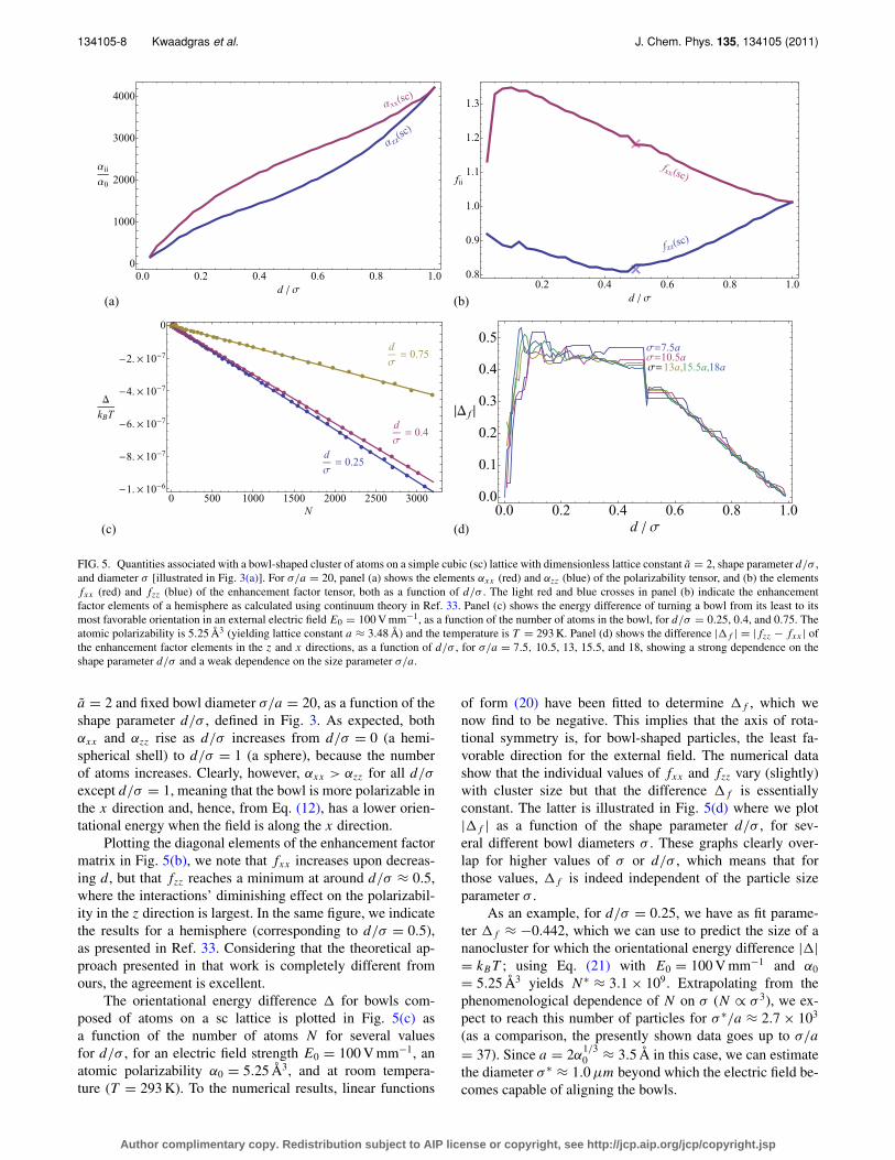
for L/σ > 1, the spheres are actually separated by a gap. Thelocations of the atoms in the clusters can be inferred by inter-secting the cluster shape with a lattice of our choice. In thepresent work, we will focus on a simple cubic lattice.52 Ex-amples of resulting clusters are depicted in Fig. 4, in whichour choice of coordinate system is also defined, such that thecluster polarizabilities are diagonal with αxx = αyy .

A. Bowls

In Fig. 5(a), we plot αxx and αzz for a bowl-shaped par-ticle, consisting of atoms on a sc lattice with lattice spacing

FIG. 4. Examples of the dipole setup for (a) a bowl (shape parameter d/σ = 0.275) and (b) a dumbbell (shape parameter L/σ = 0.55), both intersected witha simple cubic lattice. Each sphere corresponds to an inducible dipole (Lorentz atom).

Author complimentary copy. Redistribution subject to AIP license or copyright, see http://jcp.aip.org/jcp/copyright.jsp

134105-8 Kwaadgras et al. J. Chem. Phys. 135, 134105 (2011)

d

Σ0.25

d

Σ0.4

d

Σ0.75

0 500 1000 1500 2000 2500 30001. 10 6

8. 10 7

6. 10 7

4. 10 7

2. 10 7

0

N

kBT

Α zzsc

Αxx sc

0.0 0.2 0.4 0.6 0.8 1.00

1000

2000

3000

4000

d Σ

Αii

Α0

fzz sc

fxx sc

0.2 0.4 0.6 0.8 1.00.8

0.9

1.0

1.1

1.2

1.3

d Σ

fii

7.5a10.5a13a,15.5a,18a

0.0 0.2 0.4 0.6 0.8 1.00.0

0.1

0.2

0.3

0.4

0.5

d Σ

f

(c)

(b)

(d)

(a)

FIG. 5. Quantities associated with a bowl-shaped cluster of atoms on a simple cubic (sc) lattice with dimensionless lattice constant a = 2, shape parameter d/σ ,and diameter σ [illustrated in Fig. 3(a)]. For σ/a = 20, panel (a) shows the elements αxx (red) and αzz (blue) of the polarizability tensor, and (b) the elementsfxx (red) and fzz (blue) of the enhancement factor tensor, both as a function of d/σ . The light red and blue crosses in panel (b) indicate the enhancementfactor elements of a hemisphere as calculated using continuum theory in Ref. 33. Panel (c) shows the energy difference of turning a bowl from its least to itsmost favorable orientation in an external electric field E0 = 100 V mm−1, as a function of the number of atoms in the bowl, for d/σ = 0.25, 0.4, and 0.75. Theatomic polarizability is 5.25 Å3 (yielding lattice constant a ≈ 3.48 Å) and the temperature is T = 293 K. Panel (d) shows the difference |�f | = |fzz − fxx | ofthe enhancement factor elements in the z and x directions, as a function of d/σ , for σ/a = 7.5, 10.5, 13, 15.5, and 18, showing a strong dependence on theshape parameter d/σ and a weak dependence on the size parameter σ/a.

a = 2 and fixed bowl diameter σ/a = 20, as a function of theshape parameter d/σ , defined in Fig. 3. As expected, bothαxx and αzz rise as d/σ increases from d/σ = 0 (a hemi-spherical shell) to d/σ = 1 (a sphere), because the numberof atoms increases. Clearly, however, αxx > αzz for all d/σ

except d/σ = 1, meaning that the bowl is more polarizable inthe x direction and, hence, from Eq. (12), has a lower orien-tational energy when the field is along the x direction.

Plotting the diagonal elements of the enhancement factormatrix in Fig. 5(b), we note that fxx increases upon decreas-ing d, but that fzz reaches a minimum at around d/σ ≈ 0.5,where the interactions’ diminishing effect on the polarizabil-ity in the z direction is largest. In the same figure, we indicatethe results for a hemisphere (corresponding to d/σ = 0.5),as presented in Ref. 33. Considering that the theoretical ap-proach presented in that work is completely different fromours, the agreement is excellent.

The orientational energy difference � for bowls com-posed of atoms on a sc lattice is plotted in Fig. 5(c) asa function of the number of atoms N for several valuesfor d/σ , for an electric field strength E0 = 100 V mm−1, anatomic polarizability α0 = 5.25 Å3, and at room tempera-ture (T = 293 K). To the numerical results, linear functions

of form (20) have been fitted to determine �f , which wenow find to be negative. This implies that the axis of rota-tional symmetry is, for bowl-shaped particles, the least fa-vorable direction for the external field. The numerical datashow that the individual values of fxx and fzz vary (slightly)with cluster size but that the difference �f is essentiallyconstant. The latter is illustrated in Fig. 5(d) where we plot|�f | as a function of the shape parameter d/σ , for sev-eral different bowl diameters σ . These graphs clearly over-lap for higher values of σ or d/σ , which means that forthose values, �f is indeed independent of the particle sizeparameter σ .

As an example, for d/σ = 0.25, we have as fit parame-ter �f ≈ −0.442, which we can use to predict the size of ananocluster for which the orientational energy difference |�|= kBT ; using Eq. (21) with E0 = 100 V mm−1 and α0

= 5.25 Å3 yields N∗ ≈ 3.1 × 109. Extrapolating from thephenomenological dependence of N on σ (N ∝ σ 3), we ex-pect to reach this number of particles for σ ∗/a ≈ 2.7 × 103

(as a comparison, the presently shown data goes up to σ/a

= 37). Since a = 2α1/30 ≈ 3.5 Å in this case, we can estimate

the diameter σ ∗ ≈ 1.0 μm beyond which the electric field be-comes capable of aligning the bowls.

Author complimentary copy. Redistribution subject to AIP license or copyright, see http://jcp.aip.org/jcp/copyright.jsp

134105-9 Polarizability and alignment of nanoparticles J. Chem. Phys. 135, 134105 (2011)

B. Dumbbells

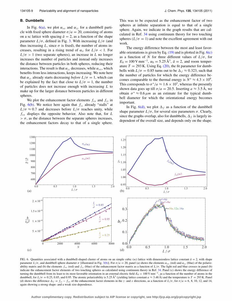
In Fig. 6(a), we plot αxx and αzz for a dumbbell parti-cle with fixed sphere diameter σ/a = 20, consisting of atomson a sc lattice with spacing a = 2, as a function of the shapeparameter L/σ , defined in Fig. 3. With increasing L/σ (andthus increasing L, since σ is fixed), the number of atoms in-creases, resulting in a rising trend of αii for L/σ < 1. ForL/σ > 1 (two separate spheres), an increase in L no longerincreases the number of particles and instead only increasesthe distance between particles in both spheres, reducing theirinteractions. The result is that αzz decreases, while αxx , whichbenefits from less interactions, keeps increasing. We note herethat αzz already starts decreasing before L/σ = 1, which canbe explained by the fact that close to L/σ = 1, the numberof particles does not increase enough with increasing L tomake up for the larger distance between particles in differentspheres.

We plot the enhancement factor elements fxx and fzz inFig. 6(b). We notice here again that fzz already “stalls” atL/σ ≈ 0.7 and decreases before L/σ reaches unity, whilefxx displays the opposite behavior. Also note that, for L

> σ , as the distance between the separate spheres increases,the enhancement factors decay to that of a single sphere.

This was to be expected as the enhancement factor of twospheres at infinite separation is equal to that of a singlesphere. Again, we indicate in the graph results that are cal-culated in Ref. 34 using continuum theory for two touchingspheres (L/σ = 1) and note the excellent agreement with outwork.

The energy difference between the most and least favor-able orientations is given by Eq. (19) and is plotted in Fig. 6(c)as a function of N for three different values of L/σ , forE0 = 100 V mm−1, α0 = 5.25 Å3, a = 2, and room temper-ature T = 293 K. Using Eq. (20), the fit parameter for dumb-bells with L/σ = 0.85 turns out to be �f ≈ 0.323, such thatthe number of particles for which the energy difference be-comes comparable to the thermal energy is N∗ ≈ 4.3 × 109.This corresponds to σ ∗/a ≈ 1.6 × 103, whereas the presentlyshown data goes up till σ/a = 20.5. Inserting a ≈ 3.5 Å, weobtain σ ∗ ≈ 0.6 μm as an estimate for the typical dumb-bell diameter for which the orientational energy becomesimportant.

In Fig. 6(d), we plot �f as a function of the dumbbellshape parameter L/σ , for several size parameters σ . Clearly,since the graphs overlap, also for dumbbells, �f is largely in-dependent of the overall size, and depends only on the shape.

Αzz sc

Αxx sc

0.0 0.5 1.0 1.5 2.0

600

700

800

900

1000

1100

1200

1300

L Σ

Αii

Α0fzz sc

fxx sc

0.0 0.5 1.0 1.5 2.00.95

1.00

1.05

1.10

1.15

1.20

1.25

L Σ

fii

L

Σ0.85

L

Σ0.95

L

Σ0.25

0 2000 4000 6000 80000

5. 10 7

1. 10 6

1.5 10 6

2. 10 6

N

kBT

6a8a

10a,12a,14a

0.0 0.5 1.0 1.5 2.00.0

0.1

0.2

0.3

L Σ

f

(c)

(b)

(d)

(a)

FIG. 6. Quantities associated with a dumbbell-shaped cluster of atoms on an simple cubic (sc) lattice with dimensionless lattice constant a = 2, with shapeparameter L/σ , and dumbbell sphere diameter σ [illustrated in Fig. 3(b)]. For σ/a = 20, panel (a) shows the elements αxx (red) and αzz (blue) of the polariz-ability matrix and (b) the elements fxx (red) and fzz (blue) of the enhancement factor matrix as a function of L/σ . The light red and blue crosses in panel (b)indicate the enhancement factor elements of two touching spheres as calculated using continuum theory in Ref. 34. Panel (c) shows the energy difference ofturning the dumbbell from its least to its most favorable orientation in an external electric field E0 = 100 V mm−1, as a function of the number of atoms in thedumbbell, for L/σ = 0.25, 0.85, and 0.95. The atomic polarizability is 5.25 Å3 (yielding lattice constant a ≈ 3.48 Å) and the temperature is T = 293 K. Panel(d) shows the difference �f = fzz − fxx of the enhancement factor elements in the z- and x directions, as a function of L/σ , for σ/a = 6, 8, 10, 12, and 14,again showing a strong shape- and a weak size-dependence.

Author complimentary copy. Redistribution subject to AIP license or copyright, see http://jcp.aip.org/jcp/copyright.jsp

134105-10 Kwaadgras et al. J. Chem. Phys. 135, 134105 (2011)

V. THE ENHANCEMENT FACTOR OF DIELECTRICCUBES

In the nonretarded limit of present interest, the inter-action energy between dipoles separated by a distance r is∝ r−3. In three dimensions, this is a long-range interactionwhich does not decay sufficiently quickly to ignore systemsize and boundary effects. Therefore, we should not expect tobe able to determine bulk quantities from calculations such asthose done in this paper. The enhancement factor difference�f (discussed in Secs. III and IV), which is found to beessentially independent of size, seems to be an interestingexception.

In Ref. 26, the enhancement factor of one-dimensionallines and two-dimensional squares of atoms was determinedand investigated in detail. For these low-dimensional systemsthe r−3 interaction is short-ranged, such that well-defined bulkbehavior is found in the “middle” of these clusters, indepen-dent of the boundary layers. In this section, we aim to do thesame for a cubic-shaped particle with atoms on a cubic lat-tice. We will confirm that the polarizability does not seemto reach a bulk value for this three-dimensional object. In-terestingly, since the fully retarded interaction energy decaysasymptotically as ∝ r−4, we may thus note that the existenceof a well-defined polarizability (and hence permittivity) forreal-life bulk substances can be qualified as a retardation ef-fect: the fact the speed of light is finite results in substanceshaving well-defined bulk permittivities.

A. Theoretical predictions

In Ref. 26, the (scalar) enhancement factor for a cubicL × L × L cluster of atoms on a cubic lattice is plotted as afunction of the rib length L. The enhancement factor is seento increase with increasing cube size, seemingly approach-ing some limiting value greater than unity. In contrast, whenit is assumed that all dipoles have the same polarization, itis possible to prove that26, 45 f (∞ × ∞ × ∞) = 1. However,by assuming the same polarization for all dipoles, we neglectthe effect of the surfaces of the cube, which is questionablegiven the long range of the dipole-dipole potential (∝ r−3).One might argue that an infinite lattice of atoms without anysurface is the best model for a bulk substance imaginable, butrealistic substances are never infinite and, as will be shown,their surfaces do have a significant effect on the polarizabilityeven when their proportional number of atoms becomes low.

In Ref. 26 the enhancement factor is plotted for cube sizesup to 10 × 10 × 10. This is still far from the regime where thesurface can be expected to be negligible; the ratio of dipoles atthe surface is, for this cube size, still (103 − 83)/103 ≈ 0.49.In the present work, we will therefore consider larger cubicclusters, of sizes up to 120 × 120 × 120. For these clusters,the fraction of surface dipoles is ∼0.05. Another predictionfor the limiting value of f (L → ∞) can be obtained fromthe Clausius-Mosotti relation. For our purposes, a convenientform of this relation is given by53

pc = Nα0E0

1 − nα0/3,

where n is the number density of atoms. For a simple cubiclattice, where the number density equals n = 1/a3, the en-hancement factor is thus given by

f = 1

1 − α0/3a3I. (25)

The Clausius-Mosotti relation is expected to give a better pre-diction for lower densities.45 Below, we will compare the pre-diction of Eq. (25) to numerical results as a function of thedimensionless lattice constant a = a/α

1/30 .

B. Numerical methods

Special optimization techniques were used in the caseof large dielectric cubes. Because the number of atoms inthe cluster increases rapidly with the rib length of the cube,we encounter practical problems such as memory limitations.However, two techniques can be used to reduce this problem,which we will now briefly discuss.

1. Exploiting symmetry

In this technique, we use the symmetries of the cube to re-duce the order of the linear equation to be solved. It is possibleto express the polarizations of all the dipoles in terms of onlythose in one octant of the cube. If we insert these relationsinto the set of Eqs. (11), we reduce the number of dipoles bya factor of 8. Note that in this way, we also increase the com-putational cost of calculating a matrix element by (roughly) afactor of 8, but since the cost of solving a set of linear equa-tions scales with the square of the order of the equation set,we gain an overall factor of 8 in computation speed.

2. The Gauss-Seidel method

The second technique uses the Gauss-Seidel method54 forsolving a set of linear equations, trading computation speedfor less memory use. The Gauss-Seidel method is an itera-tive method for solving P from an equation of form (11). Themethod starts with a guess (discussed below) for P , which weshall call P (0). The next approximation for P , P (1), is calcu-lated using the following formula:

p(k+1)i = 1

zii

⎛⎝ei −

∑j>i

zijp(k)j −

∑i>j

zijp(k+1)j

⎞⎠ , (26)

where the p(k)i are the elements of P (k), the ei are the elements

of E , and the zij are the elements of the matrix (I − α0T ).Note that in our case zii = 1, and that we can write Eq. (26)in terms of more familiar quantities,51

p(k+1)i = E0 −

∑j>i

Zij · p(k)j −

∑i>j

Zij · p(k+1)j ,

where the Zij are 3 × 3 blocks in the matrix (I − α0T ). Notethat with this technique, it is not necessary to store a “new”and an “old” copy of P , because only elements are neededthat have been calculated previously; i.e., it is no problem tosimply keep overwriting the elements of P .

Author complimentary copy. Redistribution subject to AIP license or copyright, see http://jcp.aip.org/jcp/copyright.jsp

134105-11 Polarizability and alignment of nanoparticles J. Chem. Phys. 135, 134105 (2011)

TABLE II. An overview of techniques used for calculating the polarizabilityof a cubic cluster of atoms on a simple cubic lattice, and their associatedacronyms, as used in the caption of Fig. 7. In the LAPACK methods, we loadthe elements of the matrix in memory to the numerical precision specifiedin the “Precision” column and use the routines in the LAPACK package tosolve the relevant set of linear equations. The Gauss-Seidel methods involve(re-)calculating the elements of the matrix on the fly and, starting from aninitial guess, using 20 iterations of the Gauss-Seidel method to solve the setof linear equations. The “Symmetries” column refers to whether or not thesymmetries of the dielectric cube were exploited. The “Lmax” column listsestimates for largest feasible rib lengths that each method can handle, givenour available resources.

Acronym Method Symmetries Precision Lmax

NDL LAPACK No Double 20SDL LAPACK Yes Double 40SSL LAPACK Yes Single 48NGS Gauss-Seidel No Double 60SGS Gauss-Seidel Yes Double 120

As an initial guess we construct P (0) as follows: we sumthe Zij horizontally and then solve the equation⎛

⎝ N∑j=1

Zij

⎞⎠ · p(0)

i = E0

for each p(0)i . Using this guess, the enhancement factor could

be calculated to a precision of 10 digits within 20 iterations.Since Zij can be (re-)calculated on the fly as needed

and the elements of E can be inferred using only a three-dimensional vector, we only need to store ∼3N numbers, i.e.,the elements of P . This effectively eliminates the memoryproblem. However, as a consequence, the resulting calculationis much slower than the one that uses the LAPACK routine.

By combining the two techniques (symmetry exploitationand the Gauss-Seidel method), we were able to calculate theenhancement factor for cubes as large as 120 × 120 × 120.The data points presented in Subsection V C have beencalculated using various methods, corresponding to combi-nations of applying the two aforementioned techniques. InTable II, we give an overview of these methods, and definethe acronyms that are used in the caption of Fig. 7.

The different methods have all been tested for consis-tency and the agreement between them is excellent. Computa-tionally, the most practical techniques were the SDL-methodfor small rib lengths, because of its speed and simple imple-mentation, and the SGS-method for large rib lengths, becauseof its negligible memory usage.

C. Numerical results

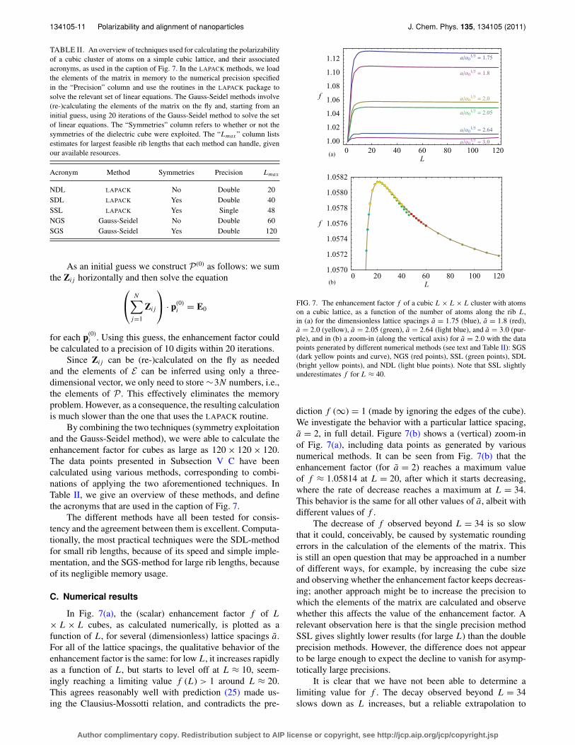
In Fig. 7(a), the (scalar) enhancement factor f of L

× L × L cubes, as calculated numerically, is plotted as afunction of L, for several (dimensionless) lattice spacings a.For all of the lattice spacings, the qualitative behavior of theenhancement factor is the same: for low L, it increases rapidlyas a function of L, but starts to level off at L ≈ 10, seem-ingly reaching a limiting value f (L) > 1 around L ≈ 20.This agrees reasonably well with prediction (25) made us-ing the Clausius-Mossotti relation, and contradicts the pre-

a Α01 3 1.75

a Α01 3 1.8

a Α01 3 2.0

a Α01 3 2.05

a Α01 3 2.64

a Α01 3 3.0

0 20 40 60 80 100 1201.00

1.02

1.04

1.06

1.08

1.10

1.12

L

f

0 20 40 60 80 100 1201.0570

1.0572

1.0574

1.0576

1.0578

1.0580

1.0582

L

f

(a)

(b)

FIG. 7. The enhancement factor f of a cubic L × L × L cluster with atomson a cubic lattice, as a function of the number of atoms along the rib L,in (a) for the dimensionless lattice spacings a = 1.75 (blue), a = 1.8 (red),a = 2.0 (yellow), a = 2.05 (green), a = 2.64 (light blue), and a = 3.0 (pur-ple), and in (b) a zoom-in (along the vertical axis) for a = 2.0 with the datapoints generated by different numerical methods (see text and Table II): SGS(dark yellow points and curve), NGS (red points), SSL (green points), SDL(bright yellow points), and NDL (light blue points). Note that SSL slightlyunderestimates f for L ≈ 40.

diction f (∞) = 1 (made by ignoring the edges of the cube).We investigate the behavior with a particular lattice spacing,a = 2, in full detail. Figure 7(b) shows a (vertical) zoom-inof Fig. 7(a), including data points as generated by variousnumerical methods. It can be seen from Fig. 7(b) that theenhancement factor (for a = 2) reaches a maximum valueof f ≈ 1.05814 at L = 20, after which it starts decreasing,where the rate of decrease reaches a maximum at L = 34.This behavior is the same for all other values of a, albeit withdifferent values of f .

The decrease of f observed beyond L = 34 is so slowthat it could, conceivably, be caused by systematic roundingerrors in the calculation of the elements of the matrix. Thisis still an open question that may be approached in a numberof different ways, for example, by increasing the cube sizeand observing whether the enhancement factor keeps decreas-ing; another approach might be to increase the precision towhich the elements of the matrix are calculated and observewhether this affects the value of the enhancement factor. Arelevant observation here is that the single precision methodSSL gives slightly lower results (for large L) than the doubleprecision methods. However, the difference does not appearto be large enough to expect the decline to vanish for asymp-totically large precisions.

It is clear that we have not been able to determine alimiting value for f . The decay observed beyond L = 34slows down as L increases, but a reliable extrapolation to

Author complimentary copy. Redistribution subject to AIP license or copyright, see http://jcp.aip.org/jcp/copyright.jsp

134105-12 Kwaadgras et al. J. Chem. Phys. 135, 134105 (2011)

1.8 2.0 2.2 2.4 2.6 2.8 3.01.00

1.02

1.04

1.06

1.08

1.10

1.12

1.14

a~

f

FIG. 8. The enhancement factor f of a 120 × 120 × 120 cube of atoms,as a function of the (dimensionless) lattice constant a = a/α

1/30 . In blue,

the numerical results are plotted, while in red, the prediction as given bythe Clausius-Mosotti relation, Eq. (25), is shown. The dashed green line isEq. (22) of Ref. 32, where the enhancement factor is calculated using contin-uum theory. Note the excellent agreement between the latter and our result,despite the completely different approaches.

asymptotically large cubes could not be determined. There-fore, bulk behavior was not reached for our cube sizes. Westress again that this conclusion was reached not based on theabsolute value of f at L = 120, but based on the variationthat we observe for large L.

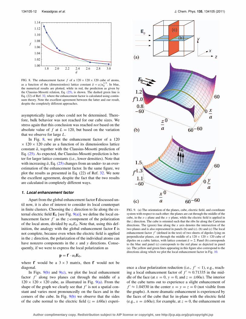
In Fig. 8, we plot the enhancement factor of a 120× 120 × 120 cube as a function of its dimensionless latticeconstant a, together with the Clausius-Mosotti prediction ofEq. (25). As expected, the Clausius-Mosotti prediction is bet-ter for larger lattice constants (i.e., lower densities). Note thatwith increasing a, Eq. (25) changes from an under- to an over-estimation of the enhancement factor. In the same figure, weplot the results as presented in Eq. (22) of Ref. 32. We notethe excellent agreement, despite the fact that the two resultsare calculated in completely different ways.

1. Local enhancement factor

Apart from the global enhancement factor f discussed un-til now, it is also of interest to consider its local counterpartin finite clusters. Choosing the z direction to lie along the ex-ternal electric field E0 [see Fig. 9(a)], we define the local en-hancement factor f ′ as the z-component of the polarizationof the local atom, divided by α0E0. Note that, using this def-inition, the analogy with the global enhancement factor f isnot complete, because even when the electric field is appliedin the z direction, the polarization of the individual atoms canhave nonzero components in the x and y directions. Conse-quently, if we were to express the local polarization as

p = f′ · α0E0,

where f′ would be a 3 × 3 matrix, then f′ would not bediagonal.

In Figs. 9(b) and 9(c), we plot the local enhancementfactor f ′ along two planes cut through the middle of a120 × 120 × 120 cube, as illustrated in Fig. 9(a). From theshape of the graph we clearly see that f ′ is not a spatial con-stant and varies most pronouncedly on the faces and in thecorners of the cube. In Fig. 9(b) we observe that the sidesof the cube normal to the electric field (z = ±60a) experi-

FIG. 9. (a) The orientation of the planes, cube, electric field, and coordinatesystem with respect to each other: the planes are cut through the middle of thecube, in the x-z plane and the x-y plane, while the electric field is applied inthe z direction. The cube is oriented such that the ribs lie along the Cartesiandirections. The (green) line along the x axis denotes the intersection of thetwo planes and is also represented in panels (b) and (c). (b) and (c) The localenhancement factor f ′ (defined in the text) of two sheets of dipoles lying onperpendicular planes, cut through the middle of a 120 × 120 × 120 cube ofdipoles on a cubic lattice, with lattice constant a = 2. Panel (b) correspondsto the blue and panel (c) corresponds to the red plane as depicted in panel(a). The yellow and green lines appearing in this figure also correspond to thedirections along which we plot the local enhancement factor in Fig. 10.

ence a clear polarization reduction (i.e., f ′ < 1), e.g., reach-ing a local enhancement factor of f ′ ≈ 0.71335 in the mid-dle of the face (at x = 0, y = 0, and z = ±60a). The interiorof the cube turns out to experience a slight enhancement off ′ ≈ 1.04530 in the center x = y = z = 0 (not visible fromthe graphs). A more dramatic enhancement is experienced bythe faces of the cube that lie in-plane with the electric field(e.g., x = ±60a); for example, at z = 0, the enhancement on

Author complimentary copy. Redistribution subject to AIP license or copyright, see http://jcp.aip.org/jcp/copyright.jsp

134105-13 Polarizability and alignment of nanoparticles J. Chem. Phys. 135, 134105 (2011)

L10L

20L50

,120

0.4 0.2 0.0 0.2 0.4

1.05

1.10

1.15

1.20

x a L

f

L 10

L 20

L 50

L 120

0 2 4 6 8 10 12 14

1.05

1.10

1.15

1.20

x a

f

L10,20,50,120

0.4 0.2 0.0 0.2 0.4

0.75

0.80

0.85

0.90

0.95

1.00

1.05

z a L

f

(a)

(b)

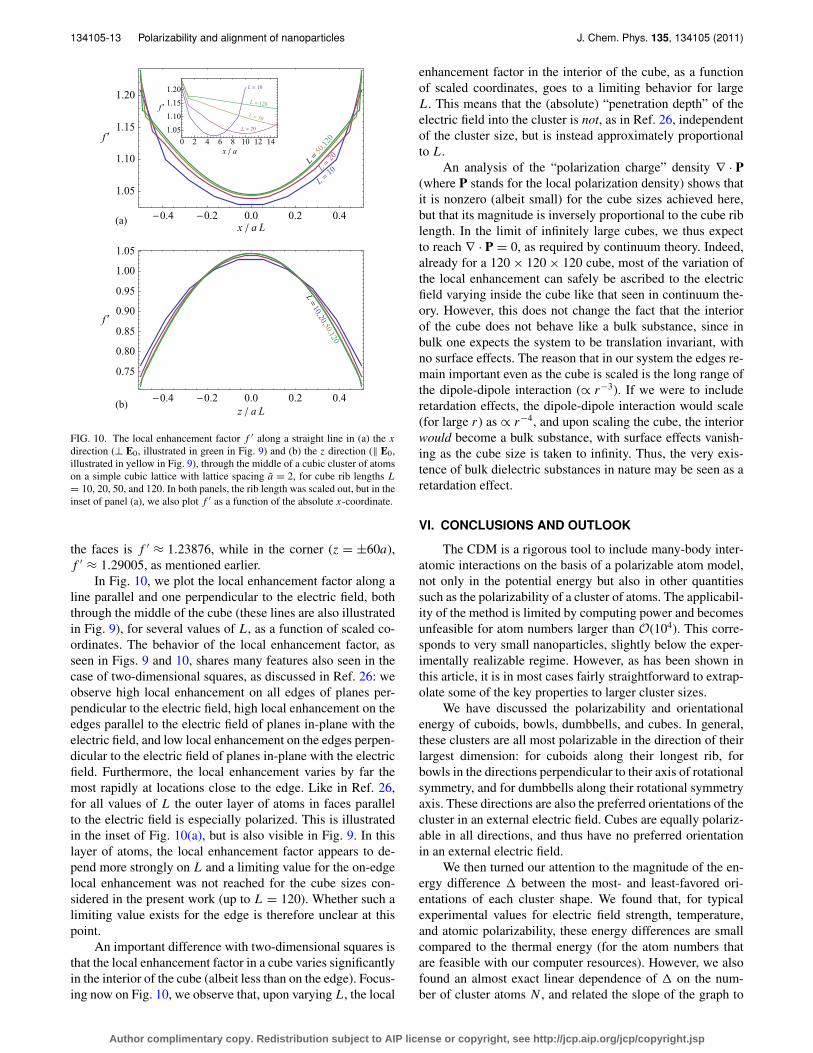
FIG. 10. The local enhancement factor f ′ along a straight line in (a) the x

direction (⊥ E0, illustrated in green in Fig. 9) and (b) the z direction (‖ E0,illustrated in yellow in Fig. 9), through the middle of a cubic cluster of atomson a simple cubic lattice with lattice spacing a = 2, for cube rib lengths L

= 10, 20, 50, and 120. In both panels, the rib length was scaled out, but in theinset of panel (a), we also plot f ′ as a function of the absolute x-coordinate.

the faces is f ′ ≈ 1.23876, while in the corner (z = ±60a),f ′ ≈ 1.29005, as mentioned earlier.

In Fig. 10, we plot the local enhancement factor along aline parallel and one perpendicular to the electric field, boththrough the middle of the cube (these lines are also illustratedin Fig. 9), for several values of L, as a function of scaled co-ordinates. The behavior of the local enhancement factor, asseen in Figs. 9 and 10, shares many features also seen in thecase of two-dimensional squares, as discussed in Ref. 26: weobserve high local enhancement on all edges of planes per-pendicular to the electric field, high local enhancement on theedges parallel to the electric field of planes in-plane with theelectric field, and low local enhancement on the edges perpen-dicular to the electric field of planes in-plane with the electricfield. Furthermore, the local enhancement varies by far themost rapidly at locations close to the edge. Like in Ref. 26,for all values of L the outer layer of atoms in faces parallelto the electric field is especially polarized. This is illustratedin the inset of Fig. 10(a), but is also visible in Fig. 9. In thislayer of atoms, the local enhancement factor appears to de-pend more strongly on L and a limiting value for the on-edgelocal enhancement was not reached for the cube sizes con-sidered in the present work (up to L = 120). Whether such alimiting value exists for the edge is therefore unclear at thispoint.

An important difference with two-dimensional squares isthat the local enhancement factor in a cube varies significantlyin the interior of the cube (albeit less than on the edge). Focus-ing now on Fig. 10, we observe that, upon varying L, the local

enhancement factor in the interior of the cube, as a functionof scaled coordinates, goes to a limiting behavior for largeL. This means that the (absolute) “penetration depth” of theelectric field into the cluster is not, as in Ref. 26, independentof the cluster size, but is instead approximately proportionalto L.

An analysis of the “polarization charge” density ∇ · P(where P stands for the local polarization density) shows thatit is nonzero (albeit small) for the cube sizes achieved here,but that its magnitude is inversely proportional to the cube riblength. In the limit of infinitely large cubes, we thus expectto reach ∇ · P = 0, as required by continuum theory. Indeed,already for a 120 × 120 × 120 cube, most of the variation ofthe local enhancement can safely be ascribed to the electricfield varying inside the cube like that seen in continuum the-ory. However, this does not change the fact that the interiorof the cube does not behave like a bulk substance, since inbulk one expects the system to be translation invariant, withno surface effects. The reason that in our system the edges re-main important even as the cube is scaled is the long range ofthe dipole-dipole interaction (∝ r−3). If we were to includeretardation effects, the dipole-dipole interaction would scale(for large r) as ∝ r−4, and upon scaling the cube, the interiorwould become a bulk substance, with surface effects vanish-ing as the cube size is taken to infinity. Thus, the very exis-tence of bulk dielectric substances in nature may be seen as aretardation effect.

VI. CONCLUSIONS AND OUTLOOK

The CDM is a rigorous tool to include many-body inter-atomic interactions on the basis of a polarizable atom model,not only in the potential energy but also in other quantitiessuch as the polarizability of a cluster of atoms. The applicabil-ity of the method is limited by computing power and becomesunfeasible for atom numbers larger than O(104). This corre-sponds to very small nanoparticles, slightly below the exper-imentally realizable regime. However, as has been shown inthis article, it is in most cases fairly straightforward to extrap-olate some of the key properties to larger cluster sizes.

We have discussed the polarizability and orientationalenergy of cuboids, bowls, dumbbells, and cubes. In general,these clusters are all most polarizable in the direction of theirlargest dimension: for cuboids along their longest rib, forbowls in the directions perpendicular to their axis of rotationalsymmetry, and for dumbbells along their rotational symmetryaxis. These directions are also the preferred orientations of thecluster in an external electric field. Cubes are equally polariz-able in all directions, and thus have no preferred orientationin an external electric field.

We then turned our attention to the magnitude of the en-ergy difference � between the most- and least-favored ori-entations of each cluster shape. We found that, for typicalexperimental values for electric field strength, temperature,and atomic polarizability, these energy differences are smallcompared to the thermal energy (for the atom numbers thatare feasible with our computer resources). However, we alsofound an almost exact linear dependence of � on the num-ber of cluster atoms N , and related the slope of the graph to

Author complimentary copy. Redistribution subject to AIP license or copyright, see http://jcp.aip.org/jcp/copyright.jsp

134105-14 Kwaadgras et al. J. Chem. Phys. 135, 134105 (2011)

the difference �f in enhancement factor diagonal elements,a quantity that turns out to be independent of the cluster sizeand that depends only on the cluster shape and lattice spacing.The dependence of �f on the cluster shape was then investi-gated. This was done for several cluster sizes in order to provethe size-independence of �f . Using the linear dependence of� on N , we estimated, for some chosen cluster shapes, thenumber of atoms (and hence the spatial dimensions of thecluster) for � to be of the order of the thermal energy. This isrelevant because it gives an estimate for when a dielectric col-loid might be aligned in an external electric field. The esti-mates, for some typical experimental parameters, all have val-ues of roughly 1 μm for the longest dimension of the colloid.In other words, dielectric nanoparticles are not easily alignedby external electric fields.

The enhancement factor of a cubic cluster of atoms ona simple cubic lattice at first glance seems to go to a well-defined asymptotic value. However, closer inspection revealsthat, in fact, the enhancement factor starts decreasing againas the rib length increases and whether a limiting value ofthe enhancement factor exists is still unclear at this point. Asshown, the local enhancement factor does not reach a plateauin the interior of the cube, even for the largest cubes, and sothe question of whether bulk behavior will be reached, judg-ing from the results presented here, seems to have “no” asan answer. This can be attributed to the long range (∝ r−3)character of the dipole-dipole interaction, and hence retarda-tion (which results in an interaction ∝ r−4) may be seen asthe cause of the well-defined bulk dielectric properties as ob-served in nature.

ACKNOWLEDGMENTS

This work is part of the research programme of FOM,which is financially supported by NWO. Financial support byan NWO-VICI grant is acknowledged.

1S. C. Glotzer and M. J. Solomon, Nature Mater. 6, 557 (2007).2S.-M. Yang, S.-H. Kim, J.-M. Lim, and G.-R. Yi, J. Mater. Chem. 18, 2177(2008).

3M. Grzelczak, J. Vermant, E. M. Furst, and L. M. Liz-Marzán, ACS Nano4, 3591 (2010).

4M. J. Solomon, Curr. Opin. Colloid Interface Sci. 16, 158 (2011).5S. C. Glotzer, M. A. Horsch, C. R. Iacovella, Z. Zhang, E. R. Chan, andX. Zhang, Curr. Opin. Colloid Interface Sci. 10, 287 (2005).

6B. Nikoobakht, Z. L. Wang, and M. A. El-Sayed, J. Phys. Chem. B 104,8635 (2000).

7D. Fava, Z. Nie, M. A. Winnik, and E. Kumacheva, Adv. Mater. 20, 4318(2008).

8E. L. Thomas, Science 286, 1307 (1999).9D. J. Kraft, W. S. Vlug, C. M. van Kats, A. van Blaaderen, A. Imhof, andW. K. Kegel, J. Am. Chem. Soc. 131, 1182 (2009).

10I. D. Hosein, S. H. Lee, and C. M. Liddell, Adv. Funct. Mater. 20, 3085(2010).

11L. Onsager, Ann. N.Y. Acad. Sci. 51, 627 (1949).12K. M. Ryan, A. Mastroianni, K. A. Stancil, H. T. Liu, and A. P. Alivisatos,

Nano Lett. 6, 1479 (2006).13D. van der Beek, A. V. Petukhov, P. Davidson, J. Ferré, J. P. Jamet,

H. H. Wensink, G. J. Vroege, W. Bras, and H. N. W. Lekkerkerker, Phys.Rev. E 73, 041402 (2006).

14K. Bubke, H. Gnewuch, M. Hempstead, J. Hammer, and M. L. H. Green,Appl. Phys. Lett. 71, 1906 (1997).

15A. F. Demirörs, P. M. Johnson, C. M. van Kats, A. van Blaaderen, andA. Imhof, Langmuir 26, 14466 (2010).

16P. A. Smith, C. D. Nordquist, T. N. Jackson, T. S. Mayer, B. R. Martin,J. Mbindyo, and T. E. Mallouk, Appl. Phys. Lett. 77, 1399 (2000).

17D. V. Talapin, E. V. Shevchenko, C. B. Murray, A. Kornowski, S. Forster,and H. Weller, J. Am. Chem. Soc. 126, 12984 (2004).

18S. Ahmed and K. M. Ryan, Nano Lett. 7, 2480 (2007).19B. Q. Sun and H. Sirringhaus, J. Am. Chem. Soc. 128, 16231 (2006).20D. Nagao, C. M. van Kats, K. Hayasaka, M. Sugimoto, M. Konno,

A. Imhof, and A. van Blaaderen, Langmuir 26, 5208 (2010).21M. Marechal, R. J. Kortschot, A. F. Demirörs, A. Imhof, and M. Dijkstra,

Nano Lett. 10, 1907 (2010).22I. D. Hosein and C. M. Liddell, Langmuir 23, 8810 (2007).23L. Rossi, S. Sacanna, and K. P. Velikov, Soft Matter 7, 64 (2011).24X. D. Wang, E. Graugnard, J. S. King, Z. L. Wang, and C. J. Summers,

Nano Lett. 4, 2223 (2004).25C. Zoldesi, C. A. van Walree, and A. Imhof, Langmuir 22, 4343 (2006).26H.-Y. Kim, J. O. Sofo, D. Velegol, M. W. Cole, and G. Mukhopadhyay,

Phys. Rev. A 72, 053201 (2005).27M. W. Cole, D. Velegol, H.-Y. Kim, and A. A. Lucas, Mol. Simul. 35, 849

(2009).28C. A. Utreras-Díaz, E. Martín García, and M. A. R. Troncoso, Phys. Status

Solidi B 190, 421 (1995).29M. Manninen, R. M. Nieminen, and M. J. Puska, Phys. Rev. B 33, 4289

(1986).30W. D. Knight, K. Clemenger, W. A. de Heer, and W. A. Saunders, Phys.

Rev. B 31, R2539 (1985).31A. Sihvola, J. Nanomater. 2007, 45090 (2007).32A. Sihvola, P. Ylä-Oijala, S. Järvenpää, and J. Avelin, IEEE Trans. Anten-

nas Propag. 52, 2226 (2004).33H. Kettunen, H. Wallén, and A. Sihvola, J. Appl. Phys. 102, 044105

(2007).34M. Pitkonen, J. Appl. Phys. 103, 104910 (2008).35M. Pitkonen, J. Math. Phys. 47, 102901 (2006).36M. J. Renne and B. R. A. Nijboer, Chem. Phys. Lett. 1, 317 (1967).37B. R. A. Nijboer and M. J. Renne, Chem. Phys. Lett. 2, 35 (1968).38M. W. Cole and D. Velegol, Mol. Phys. 106, 1587 (2008).39F. London, Z. Phys. 63, 245 (1930).40I. E. Dzyaloshinskii, E. M. Lifshitz, and L. P. Pitaevskii, Adv. Phys. 10, 165

(1961).41H. C. Hamaker, Physica 4, 1058 (1937).42J. H. de Boer, Trans. Faraday Soc. 32, 10 (1936).43B. Derjaguin and L. Landau, Acta Physicochim. URSS 14, 633 (1941).44E. J. W. Verwey and J. T. G. Overbeek, Theory of the Stability of Lyophobic

Colloids (Elsevier, New York, 1948).45J. D. Jackson, Classical Electrodynamics, 3rd ed. (Wiley, New York,

1999).46H.-Y. Kim, J. O. Sofo, D. Velegol, M. W. Cole, and A. A. Lucas, J. Chem.

Phys. 124, 074504 (2006).47S. M. Gatica, M. W. Cole, and D. Velegol, Nano Lett. 5, 169 (2005).48H.-Y. Kim, J. O. Sofo, D. Velegol, M. W. Cole, and A. A. Lucas, Langmuir

23, 1735 (2007).49This proof relies on the fact that Dij = DT

ij , which, in turn, can be proven byusing induction in combination with the general expression for the inverseof a matrix built up of submatrices:

(K LM N

)−1

=(

K−1 + K−1LS−1MK−1 −K−1LS−1

−S−1MK−1 S−1

),

where

S = (N − MK−1L).

50See http://www.netlib.org/lapack/ for information and downloadableversions of LAPACK.

51From Eq. (18), we could also have derived an explicit expression for theorientational energy of the cluster shapes discussed in this article:

VE = − 1

2[(E0 · x)2 + (E0 · y)2]αxx − 1

2(E0 · z)2αzz

= − 1

2(αxx + (αzz − αxx ) cos2 θ )E2

0 ,

where in the first line we used αxx = αyy and in the second line, we intro-duced the angle θ between E0 and the z axis. From the resulting expression,

Author complimentary copy. Redistribution subject to AIP license or copyright, see http://jcp.aip.org/jcp/copyright.jsp

134105-15 Polarizability and alignment of nanoparticles J. Chem. Phys. 135, 134105 (2011)

it is clear that the extrema of the orientational energy are located at θ = 0and θ = π/2 and that the difference in orientational energy between thetwo extrema is indeed given by Eq. (19).

52For bowls and dumbbells, calculations were also done using a face-centeredcubic lattice. The results are qualitatively the same. Quantitatively, the en-hancement factors tend to differ from unity more with an fcc lattice thanwith a sc lattice, which can be attributed to the higher density of atoms,

resulting in stronger atom-atom interactions and hence stronger many-bodyeffects.

53J. H. Hannay, Eur. J. Phys. 4, 141 (1983).54R. Barrett, M. Berry, T. F. Chan, J. Demmel, J. Donato, J. Dongarra, V.

Eijkhout, R. Pozo, C. Romine, and H. van der Vorst, Templates for theSolution of Linear Systems: Building Blocks for Iterative Methods (SIAM,Philadelphia, 1994).

Author complimentary copy. Redistribution subject to AIP license or copyright, see http://jcp.aip.org/jcp/copyright.jsp