On the thermohaline variability of the Baltic Sea

Ž .Journal of Marine Systems 25 2000 333–357www.elsevier.nlrlocaterjmarsys

On the thermohaline variability of the Baltic Sea

Andreas Lehmann), Hans-Harald HinrichsenInstitut fur Meereskunde Kiel, Dusternbrooker Weg 20, D-24105 Kiel, Germany¨ ¨

Received 15 November 1998; accepted 16 July 1999

Abstract

A coupled ice–ocean model is utilized to investigate the transports of heat, salt and water in the Baltic Sea for the years1986, 1988, 1993 and 1994. The oceanic component of the coupled system is a three-dimensional baroclinic model of theBaltic Sea including the Belt Sea and the SkagerrakrKattegat area. The model has a horizontal resolution of ;5 km and 28vertical levels specified. The ice model is based on the Hamburg Sea Ice model, with the same horizontal resolution. The

Žcoupled system is driven by atmospheric data provided by the Swedish Meteorological and Hydrological Institute SMHI;.Norrkoping, Sweden and river runoff taken from a monthly mean runoff database. The thermohaline variability of the Baltic¨

Sea strongly depends on the fluctuations of the atmospheric forcing conditions. Therefore, high demands on the spatial andtemporal resolution of the meteorological forcing are required. Besides heat and radiation fluxes, precipitation andevaporation rates have to be taken into account. From the coupled runs, the different components determining the energy andwater cycle of the Baltic Sea are identified and estimates of the water, heat and salt transports are given for the differentyears. Furthermore, the thermohaline variability is investigated with respect to the relevant forcing mechanisms includingatmospheric, as well as fresh water fluxes. Besides the heat and water fluxes of the Baltic Sea and the water mass exchangewith the North Sea, internal fluxes of heat, salt and volume between the different subbasins of the Baltic Sea are presented.Sensitivity studies on the variation of the net fresh water flux indicate that uncertainties in precipitation andror river runoffcan have a strong impact on the inflow of highly saline water from the North Sea, thus, influencing the thermohalinecirculation of the Baltic Sea. q 2000 Elsevier Science B.V. All rights reserved.

Keywords: salt flux; heat flux; ocean currents; numerical model; Baltic Sea

1. Introduction

The investigation of the energy and water budgetof the Baltic Sea and its catchment area is one main

Ž .aim of BALTEX Baltic Sea Experiment, 1995 . Theunderstanding of the role of the Baltic Sea in energyand water cycles requires models for the relevant

) Corresponding author. Tel.: q49-431-597-4013; fax: q49-431-565-876.

Ž .E-mail address: [email protected] A. Lehmann .

transport processes. The modelling efforts withinBALTEX are directed towards the development andverification of models, which describe relevant com-ponents of the energy and water cycle in the BAL-TEX region. The models must be suitable to describethe physical state of the Baltic Sea in response toatmospheric and hydrological forcing, including itsvariability on time scales from weeks to decades, andon spatial scales ranging from 10–20 km to theentire basin size. With respect to the water budget,the models must be able to describe the transport of

0924-7963r00r$ - see front matter q 2000 Elsevier Science B.V. All rights reserved.Ž .PII: S0924-7963 00 00026-9

( )A. Lehmann, H.-H. HinrichsenrJournal of Marine Systems 25 2000 333–357334

water and salt through the Danish Straits whichrequires an understanding of the dynamics of the in-and outflow processes and of the thermohaline circu-lation and mixing processes which determine thelong-term distribution of water masses in the Baltic

ŽSea e.g. Stigebrandt, 1987; Liljebladh and Stige-.brandt, 1996 . Besides short-term modelling of spe-

cific hydrographic situations with reasonable initialŽ .conditions for the sea state Hinrichsen et al., 1997 ,

simulations which cover time scales from years todecades need at least ice to be additionally consid-

Žered Zhang and Lepparanta, 1995; Haapala and¨Lepparanta, 1996; Omstedt and Nyberg, 1996;¨

.Schrum, 1997 . Due to the strong interaction ofatmosphere, ice and ocean, a quantification of thefluxes between the components requires the utiliza-

Ž .tion of coupled numerical models Fig. 1 . From theoceanographic point of view, the components ice,ocean and atmosphere are strongly interacting,whereas, to the hydrology less distinct re-couplingexists. The atmosphere provides the forcing for theice–ocean system, namely, momentum, salt and heatfluxes which include precipitation, evaporation andradiation. A re-coupling of the ocean to the atmo-sphere is provided by sensible and latent heat fluxes.In case of sea ice, the oceanic heat flux to theatmosphere is strongly reduced or even prevented.

Fig. 1. Fluxes in a coupled atmosphere–ice–ocean system.

However, the back-scattered short-wave radiation isstrongly affected by the increased albedo. In case ofopen water, the atmospheric fluxes can act directlyon the ocean surface, and in case of ice, the fluxesact on the ice surface and the ocean receives amodified forcing, depending on ice dynamics, thick-ness and compactness. The ocean, in turn, suppliesheat and momentum fluxes to the lower ice surface,thereby strongly modifying the ice evolution. The netfresh water flux, which is a combination of evapora-tionrprecipitation and river runoff is a further com-ponent which has a strong impact on the water massexchange with the North Sea and the salinity distri-

Ž .bution within the Baltic Sea Backhaus, 1996 . Riverrunoff has a regional impact on the local salinitydistribution, and due to its volume flow and dynam-ics, also affects the transports through the DanishStraits.

Although the Baltic Sea can be regarded as one ofthe most intensive observed marine areas, mean cir-culation, fluxes of heat, salt and water between thesubbasins, as well as the net volume exchange withthe North Sea are hardly known. Since 1986Ž .HELCOM , only a few investigations focused onthe heat and water balance of the Baltic Sea. Re-

Ž .cently, Omstedt and Rutgersson 2000 summarizedestimations of the energy and water cycle of the totalBaltic Sea and provided own estimations based on

Žthe PROBE–Baltic model Omstedt and Nyberg,. Ž .1996 . Hakansson 1999 calculated from a hydraulic

model a 20-year record of volume flow exchangebetween North and Baltic Sea and presented an

Ž .attempt to close the Baltic Sea water BSW budget.The BALTEX program aims at the understanding

and quantification of the energy and water cycle ofthe Baltic Sea catchment area, thus, requiring anenhanced understanding of the thermohaline circula-tion in the Baltic Sea. The work presented is acontribution to the BALTEX program. The under-standing of the circulation and the transport of heat,salt and water in the Baltic Sea is not only ofimportance for marine physics, it is also of interestfor marine biology and sedimentology and providesbackground informations for ecosystem behaviour.

The present study is based on three-dimensionalnumerical simulations of the Baltic Sea with thepurpose of providing more information about thethermohaline circulation, the three-dimensional water

( )A. Lehmann, H.-H. HinrichsenrJournal of Marine Systems 25 2000 333–357 335

mass distribution and the water, heat and salt trans-ports in response to the variability of the physicalforcing conditions. The area under investigation ex-tends from the SkagerrakrKattegat regime and theBelt Sea to the deep eastern basins of the Baltic Seaincluding the Gulf of Bothnia, the Gulf of Finland,as well as the Gulf of Riga.

The paper is organized as follows. In Section 2, adescription of the coupled ice–ocean model is given.This is followed by a description of the initial condi-tions, the forcing and the experimental design. Then,a detailed analysis of the circulation, the fluxesbetween the subbasins and the exchange with theNorth Sea is given. The paper is closed by a sum-mary and conclusions.

2. Coupled ice–ocean model

The approach used in constructing the ice–oceansystem was to couple an existing dynamic–thermo-

Ždynamic sea ice model Hibler, 1979; Stossel and¨.Owens, 1992 with a multi-level baroclinic ocean

model. The ocean model is a three-dimensional baro-clinic model of the whole Baltic Sea, with a horizon-tal resolution of 5 km and 28 vertical levels specifiedŽ .Lehmann, 1995 . The model is based on the free-

Žsurface Bryan–Cox–Semtner model Killworth et.al., 1991 which is a special version of the Cox

Žnumerical general circulation model Bryan, 1969;.Semtner, 1974; Cox, 1984 . The coupling mecha-

nisms between ice and ocean are given by momen-tum, salt and heat fluxes. Ice and ocean models aredirectly coupled, i.e. the information exchange takesplace via the upper ocean level, with no specialmixed layer model in between. The coupled systemis driven by atmospheric data provided by theSwedish Meteorological and Hydrological InstituteŽ .SMHI; Norrkoping, Sweden Meteorological¨

Ž .database Lars Meuller, personal communication andriver runoff taken from a mean runoff databaseŽ .Bergstrom and Carlsson, 1994 .¨

The main problem in setting up the coupled ice–ocean model is to find appropriate parameterizationsfor the corresponding fluxes responsible for driving

Ž .the system Fig. 1 , namely, momentum, latent andsensible heat fluxes, fresh water and radiation fluxes.In case of an ice-free ocean, these fluxes act directly

on the ocean surface, in case of ice, they act on theice surface and the ocean receives a modified forcingdepending on ice dynamics, ice thickness and con-centration, and an additional snow cover.

The coupling procedure of the ice and oceanmodel will be given here, a description of the ocean

Ž .model can be found in Lehmann 1995 , and of theŽ .ice model in Stossel and Owens 1992 . The govern-¨

ing equations, along with their boundary conditions,are solved by finite difference technique with a

Žstaggered ‘‘B’’ grid configuration Mesinger and.Arakawa, 1976 . The time differencing of the ocean

model is centered, i.e. leapfrog. However, the schemeis quasi-implicit in that the vertical diffusion is eval-uated at the forward time level. Thus, small verticalspacing is permissible near the surface without theneed to reduce the time increment or restrict themagnitude of the mixing coefficient. For the solutionof the ice momentum equations, a semi-implicit pre-dictor–corrector procedure is used to center the non-linear terms. Under this procedure, two relaxationsolutions are required at each time step, one to thenonlinear terms and one to advance to the next timestep. In each case, point relaxation techniques areused to solve the linearized implicit equations.

The coupled system is synchronously integratedin time, i.e. time steps of ice and ocean models arethe same. First, with the atmospheric forcing and theocean surface current, sea surface tilt, salinity andtemperature of the actual time step, the ice model isintegrated forward in time, providing the surfacestress to the ocean model where the ocean is icecovered. In ice-free areas, the atmospheric surfacestress acts directly on the ocean surface. The com-bined atmospheric–ice stress drives then the oceanmodel.

The ice model is coupled to the top layer of theocean model via the fluxes of momentum, heat andsalt. The stresses at the ice–ocean interface read:

< <t sr c u yu u yu cosfŽ .io o dio i o i o 0

qk= u yu sinf 1Ž . Ž .i o 0

t s 1yA t qAt , 2Ž . Ž .s a io

with the wind stresses on the ice and ocean surfaces,

< <t sr c V V 3Ž .ai a dai w w

< <t sr c V V . 4Ž .ao a dao w w


Here, c , c and c denote the drag coefficientsdio dao dai

for the ice–ocean, atmosphere–ocean and atmo-sphere–ice interface, f , assumed to be zero, is the0

Ž .turning angle between ice u and surface oceaniŽ .velocity u , and r represents the ocean referenceo 0

density. t is the surface stress resulting from thesŽ . Ž .ice–ocean movement t and the wind stress t ,io a

where A denotes the ice compactness, which is 1 ifthe grid box is totally ice covered and zero in thecase of no ice. The boundary condition at the ocean

Ž .surface zs0 is

Eu EÕx yr K , s t ,t , 5Ž .Ž .0 M s sž /Ez Ez

with K as the eddy viscosity. Thus, the oceanM

model is driven by the combined ice–ocean–atmo-sphere surface stress. Because the ice model is onlytwo-dimensional, the atmospheric and ice–oceansurface stresses are included in the ice momentumbalance.

In the thermodynamic part of the ice–oceanmodel, the heat balance equation is solved separatelyfor the open water and the ice-covered part of a gridcell. The conservation equations for the ice–ocean

Ž .system read in rectangular coordinates below :Ž .a ice:

Ehsy= P u h qS h , A qdiffusion, 6Ž . Ž . Ž .H i h

Et

Ehsnsy= P u h qS h , A qdiffusion,Ž . Ž .H i sn sn sn

Et7Ž .

where h and h are the average ice and snowsn

thickness per unit area, S and S are thermody-h sn

namic source or sink terms. A further continuityequation is carried for the ice compactness A, ac-cording to

E Asy= P u A qS qdiffusion, 8Ž . Ž .H i A

Et

where AF1. The diffusion terms are small andintroduced solely for numerical purposes. A detaileddescription on the S , S and S can be found inh sn A

Ž .Stossel and Owens 1992 .¨

Ž .b ocean:

E ET q= P T u q TwŽ . Ž . Ž .H o

Et Ez

E ET 1 EI2s K qA = Tq 9Ž .H H hž /Ez Ez r c Ez0 p

E Es q= P su q swŽ . Ž . Ž .H o

Et Ez

E Es2s K qA = s, 10Ž .H H hž /Ez Ez

with T and s representing the three-dimensionalfields of temperature and salinity, K and A , theH H

vertical and horizontal eddy diffusivities, respec-tively. The boundary conditions at the ocean surfaceŽ .zs0 are

ET 1K s AS L q 1yA Q 11Ž . Ž .H h i u

Ez r c0 p

EsK sAS sys q 1yA s EyP , 12Ž . Ž . Ž . Ž .H h i

Ez

with s as the sea ice salinity and L as the latenti i

heat of sea ice.The growth rate S is determined from a full heath

budget calculation using bulk aerodynamic formulasfor sensible and latent heat exchanges together withincoming longwave and shortwave radiation and the

Žheat conductive flux through the ice e.g. Parkinson.and Washington, 1979 . The second term on the

Ž .right hand side in 11 denotes the heat exchangethrough the atmosphere–ocean boundary in the ab-sence of ice, where Q is the net surface heat fluxinto the oceanic mixed layer.

QsQ yQ , 13Ž .s u

where Q is the downward flux of solar radiationsŽ .and Q is the net upward flux as used in 11 ,u

Q sQ qH qH , 14Ž .u B S L

where Q is the net longwave radiation emitted fromB

the sea surface. H and H are the sensible andS L

latent heat fluxes from the sea surface to the atmo-sphere.


The shortwave radiation is approximated by theŽempirical Zillman-formula for clear skies Zillman,

.1972 :

Scos2ZR s ,sw y3cosZq2.7 e=10 q1.085cosZq0.10Ž .

15Ž .Ž y2 .with S as the solar constant 1368 W m , Z as the

Ž .sun zenith angle and e as the vapour pressure Pa .The shortwave radiation flux at the ocean surface,together with the modification due to cloudy skies isparameterized by:

Q s 1ya R 1y0.75cl , 16Ž . Ž . Ž .s sw

where as0.03 is the albedo at the ocean surfaceand cl is the fractional cloud coverage.

The net longwave radiation is due to atmospheri-Ž . Ž .cal R and water surface R radiation. Follow-l lw

Ž .ing Omstedt 1990 , this formula reads:

Q sR yRB l lw

4 4 2'se s T yT a qa e 1qa cl ,Ž .Ž .w s sea air 1 2 3

17Ž .Ž .where ´ 0.97 is the emissivity of the waterwŽ y8 y2 y4.surface, s 5.67=10 W m K is the Stefans

Boltzman’s constant. a , a and a are constants1 2 3

equal to 0.68, 0.0036 and 0.18, respectively. Thesensible and latent heat fluxes are caused by thetemperature and moisture differences between oceanand atmosphere. Their parameterizations can be writ-ten as:

H sr c C V T yT 18Ž . Ž .S air p H w sea air

H sr LC V q yq , 19Ž . Ž .L air E w 0 10

Ž y3 .with r as the air density 1.25 kg m , c repre-air p

sents the specific heat of air at a constant pressureŽ y1 y1.1004 J kg K , V is the wind velocity, T andw air

T represent the observed temperatures of the airsea

and the sea surface, respectively. L is the latent heatŽ 6 y1.of evaporation 2.5=10 J kg , C and C repre-H E

sent the transfer coefficients for sensible and latentheat, which are determined according to Isemer and

Ž .Hasse 1987 . q and q represent the specific10 0

humidities at 10 m and at the sea surface.The fresh water flux between ocean and atmo-

sphere is the result of the net effect of precipitation

Ž . Ž .P and evaporation E , where the precipitationrates are specified from the atmospheric forcing, andthe evaporation rates are approximated by:

EsH r Lr . 20Ž . Ž .L 0

Ž .Following Paulsen and Simpson 1977 , the parame-terization of absorption of downward irradiance isgiven by

I z sQ Rexp zrz q 1yR exp zrz ,Ž . Ž . Ž . Ž .s 1 2

21Ž .

where z and z are attenuation lengths and R is an1 2Ž .empirical constant. Jerlov 1968 has classified

oceanic and coastal water according to their opticalproperties. He defined five types of oceanic waterand five types of coastal water varying from cleartype to increasingly turbid. We choose the valuesRs0.64, z s0.35 and z s4.0, which correspond1 2

to coastal water type 3. The divergence of the down-ward irradiance may be written as

EI, 22Ž .

Ez

Ž .which is included as a source term in 9 .The assumption to determine the growth rates and

heat exchanges is that the velocity shear between iceand ocean will mix the first ocean model level, andhence, this mixed layer will be at the freezing tem-perature when any ice is present. The ocean transfersheat to the ice by warming up the upper level of theocean model. This heat is used to melt ice until themixed layer returns to freezing, or to warm up themixed layer if no ice is present. The ice model, inturn, is used to calculate energy exchanges with theatmosphere, based on the use of a complete surfaceheat budget. In the presence of ice, all of the heatexchanges do not transfer heat from the ocean to theatmosphere and vice versa, rather, they transfer heatto the atmosphere at the expense of the latent heat offusion of sea water via ice formation and melting.

3. Atmospheric forcing and river runoff

The meteorolgical database covers the wholeBaltic Sea drainage basin with a grid of 1=18

squares. Meteorological parameter, such as geo-


strophic wind, 2-m air temperature, 2-m relativehumidity, surface pressure, cloudiness and precipita-tion are stored with a temporal increment of 3 h. Thedatabase was created by the SMHI and covers thetime period from 1979 to 1996. The observations ofall available synoptic weather stations, together withselected ship observations were interpolated onto the1=18 grid by objective analysis. The number ofsynoptic sea observations are dominated by landstations, i.e. the atmospheric parameters over theopen sea may be biased to land conditions: the 2-mair temperature and the relative humidity show astrong daily cycle, and the precipitation rates may be

overestimated. However, the database is unique forthe Baltic Sea and includes severe, as well as mildwinters, and the long period without any stronginflow which was interrupted by the major Balticinflow in January 1993.

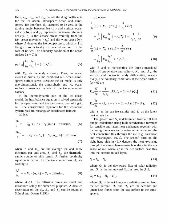
The years, which were chosen for coupled ice–ocean simulations, differ significantly from their

Ž .overall atmospheric conditions Fig. 2a-d . The year1986 was characterized by severe winter conditions,with almost the total area of the Baltic Sea frozen. In1994, there was a normal winter with about 50% ofthe Baltic Sea ice covered. 1988 and 1993 are re-garded as mild winters with ice only in the most

Ž Ž . Ž .Fig. 2. Spatial averages over the Baltic Sea of atmospheric conditions 2-m air temperature 8C , precipitation mmrday , wind velocityŽ . Ž .. Ž . Ž . Ž . Ž .mrs and direction 8 for the years a 1986, b 1988, c 1993 and d 1994.


Ž .Fig. 2 continued .

northern and eastern parts of the Baltic Sea. In 1988,especially during spring and summer, relatively longperiods with winds from northerly and easterly direc-tions were registered. In January 1993, the recent

Žmajor Baltic inflow to the Baltic Sea occurred Huberet al., 1994; Matthaus and Lass, 1995; Liljebladh and¨

.Stigebrandt, 1996 . Additionally, inflow of somemagnitude occurred in March and December, whereasminor inflows also took place in April, June and

Ž .October 1993 Hakansson, 1999 . During the inflowevents, westerly winds were prevailing interrupted

Ž .by periods of persistent easterly winds Fig. 2c ,during which larger volumes of BSW were exportedŽ .Hakansson, 1999 . The year 1994 may be character-

ized by exceptionally summer conditions, with seasurface temperatures as high as 218C.

The prescribed river runoff is taken from aŽmonthly mean database Bergstrom and Carlsson,¨

.1994 with the seasonal runoff signal included butthe inter-annual changes disregarded. HakanssonŽ .1999 showed that on the inter-annual scale, there isa clear correlation of the runoff variability with theexport of BSW to the Kattegat. To consider only theseasonal runoff signal, disregarding the inter-annualvariability simplifies the system and allows to con-centrate the analysis on the impact of the variationsof the atmospheric conditions on the circulation andtransport of heat, salt and water. The prescribed river



runoff contributes to the fresh water budget by avolume of about 450 km3ryear.

4. Experimental strategy and initial conditions

The overall aim of the numerical experiments isto determine the transports of heat, salt and water ofthe Baltic Sea in response to atmospheric and hydro-logical forcing. A number of experiments have beenperformed to investigate the impact of the atmo-spheric variability on the energy and water cycle ofthe Baltic. Four different years, namely 1986, 1988,

1993 and 1994, have been simulated starting fromthe same initial fields for the prognostic variables.The initial fields are representative for a wintersituation in the Baltic Sea. The three-dimensionalsalinity and temperature distributions resemble the

Žmonthly mean winter distribution Lenz, 1971; Bock,.1971 of the Baltic Sea, with the fields already

dynamically adjusted by a previous model run. Noinitial ice coverage was prescribed, and the riverrunoff specified was the same for each experiment.To start the different model runs from the sameinitial fields and to utilize the same amount of riverrunoff for each experiment has the advantage to



purely investigate the impact of the atmosphericforcing on the volume transport and on the thermo-haline circulation of the Baltic Sea.

5. Baltic Sea response to atmospheric and hydro-logical forcing

5.1. Mean sea surface topography

The mean inclination of the Baltic Sea surface is aconsequence of the mean density stratification whichis dominated by the salinity distribution. Due to high

Ž 3 .river runoff ;450 km ryear and a more-or-less

continuous inflow of haline water through the Dan-ish Straits, a permanent inclined halocline is main-tained. As the vertical average of salinity of theBaltic decreases from west to north and east, the sea

Ž .surface elevation increases Backhaus, 1996 . Theheight difference between the inner part of the Gulfof Bothnia and the Skagerrak amounts to 34–40 cmŽ .Fig. 3 . There is a steep sea level gradient in theborder zone between Kattegat and Skagerrak, reach-ing 2 cm per 10 km. This reflects the salinity frontthere, separating the brackish BSW from the salineNorth Sea water, and the associated Baltic current.The annual average of the sea surface elevationcalculated from the oceanographic model is in good


Ž .Fig. 3. Annual average of the simulated sea surface elevation cm for 1993.

agreement with the mean surface topography calcu-lated geodetically from long-term sea level stationsŽ .Ekman and Makinen, 1996 . Thus, the mean or¨background density stratification of the model simu-lations is in good agreement with observations.

From the variability of the spatial-averaged seasurface elevation, the total volume change of theBaltic Sea can be calculated. Landsort tide gauge isknown to be representative for the spatial-averaged

Ž .sea surface elevation Lisitzin, 1974; Jacobsen, 1980 ,thus, giving an estimate of the total volume changeof the Baltic Sea. The simulated sea surface eleva-tion at Landsort for 1993 is compared with observa-

Ž .tions from Landsort tide gauge Fig. 4 . The simu-

lated sea surface elevations agree fairly well with themeasurements implying a reasonable simulation ofthe total volume change of the Baltic Sea.

5.2. Mean circulation and Õolume transport

Due to the ephemeral nature of the meteorologicalforcing, there is no evidence of a permanent currentsystem in the Baltic Sea. In spring and early sum-mer, wind forcing is weak, thus, the circulation ismostly determined by the baroclinic field. In autumnand winter, strong westerly winds are prevailing, andthe circulation is controlled by Ekman dynamics and


Ž . Ž .Fig. 4. Simulated broken line and observed full line sea surface elevation at Landsort tide gauge for 1993.

the basin-like bottom topography superimposing theŽ .baroclinic current Krauss and Brugge, 1991 . The¨

annual mean of the barotropic circulation for thesimulated years shows only minor deviations. For allyears, there are cyclonic circulation cells comprisingeach subbasin and the Baltic Proper. The main dif-ferences of the circulation patterns between differentyears are due to the strength of the circulation cells,which is a direct result of the wind forcing during a1-year period. As an example, the annual average ofthe barotropic velocity field for 1993 is displayed inFig. 5. There is a cyclonic circulation which com-prises the Bornholm and Gotland Basin, with waterentering by a branch from the Gulf of Finland and

˚through the Aland Sea. Through the Bornholm Gat,water is leaving this circulation cell with a furtherflow through the Arkona Sea and the Danish Straitsfeeding the Baltic current. Within the subbasins,

there are cyclonic circulation patterns with the nettransport between the basins approximately deter-mined by the river runoff into the subbasin. Theinternal barotropic circulation between Gotland and

Ž 3 .Bornholm Basin 1000–2000 km ryear is about anorder of magnitude higher compared with the total

Ž 3 .river runoff to the Baltic Sea 450 km ryear . Themain fraction of water exchange between Bornholmand Gotland Basin occurs through the Stolpe Chan-nel at the southern branch of a cyclonic circulationcell comprising the Baltic Proper. From the annualaverages, it is evident that the transports along theStolpe Channel are predominantely directed from theBornholm into the Gotland Basin. Although highlyvariable between the years, this area shows mostintense transport rates of the whole Baltic Sea. Fur-thermore, it is obvious, that the lower branch of theturnover will happen through the Stolpe Channel.


Ž .Fig. 5. Annual average of the barotropic velocity cmrs for 1993.

On the long-term annual average, the water vol-ume which is supplied by the river runoff leaves theBaltic Sea through the Danish Straits. Thus, the netvolume flow from the Baltic Sea into the North Seacorresponds to the river runoff modified by the neteffect of precipitation minus evaporation.

The annual averages of the surface and nearbottom current field are displayed in Figs. 6 and 7.The surface velocity field strongly differs from thebarotropic current field reflecting a surface circula-tion which is determined by Ekman dynamics. Thecirculation patterns, as well as the absolute-value of

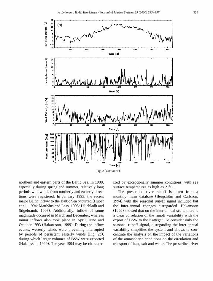
the current velocities, agree well with surface veloc-Žity maps produced from current observations Fig. 8;

.Sjoberg, 1992 . The annual average of near bottom¨velocities reflects higher currents in shallow areas,and less bottom currents in the deeper parts of thesubbasins which strongly coincides with areas where

Ž .sediment depostion will occur Fig. 8; Sjoberg, 1992 .¨It should be noted that relatively high bottom veloci-ties occur in the Danish Straits, Bornholm Gat and inthe Stolpe Channel reflecting the important role ofthese straits with respect to the water mass exchangeand thermohaline circulation.


Ž .Fig. 6. Annual average of the sea surface velocity cmrs for 1993.

5.3. Heat, salt and Õolume transports

In order to determine the transports of heat, saltand water between the Baltic Sea and theKattegatrSkagerrak area, and within the subbasinsfor the years considered, simulated velocities along

Ž .14 hydrographic sections Fig. 9 perpendicular tothe estimated main stream directions were extractedfrom model flow fields at six hourly intervals. Hori-zontal and vertical scales of the cross-section werechosen in accordance of the model’s three-dimen-sional resolution. In order to take into account the

occurrence of water masses of different character inthe Baltic Sea, additionally, corresponding transportcalculations were performed separately for watermasses having their origin in the central Baltic SeaŽ .BSW , sF10 psu , as well as in the western Baltic

ŽSea and in the KattegatrSkagerrak area KW —.Kattegat Water, s)10 psu .

The in- and outflow regime of the Baltic entranceŽ .area is represented by sections 1–4 Table 1 con-

necting the area south of Skagen with the Swedishcoastal area near Gothenborg and representing thetransports in the area of the Danish Straits.


Ž .Fig. 7. Annual average of the near bottom velocity cmrs for 1993.

To explicitely identify the annual variations ofvolume, heat and salt fluxes, further examinations ofthe influence of short- and medium scale meteoro-logical features in specific oceanographic regionswere carried out. As examples, time series of thefluxes through the Danish Straits, across the Born-holm Gat and the Rønne Bank and through theStolpe Trench were analysed.

To assess the quantitative validity of the transportcalculations based on six hourly model analysis data,we calculated the differences between the volumetransport imbalances and the change in volume stor-

age of the whole Baltic Sea. Taking into account allconsidered years, the uncertainty of our estimationsresults in 0.13 km3 with a standard deviation of 5km3.

( )5.3.1. Kattegat and Belt Sea sections 1–4For the years 1986, 1988 and 1993, the net out-

flowing volume of water is in the order of theŽ 3 .prescribed river runoff 450 km ryear . For the nu-

merical experiments, the annual river runoff wasŽheld constant, whereas the net precipitation precipi-

.tation minus evaporation varied due to the variabil-


Fig. 8. Annual mean values of the direction and speed of the surface currents. Where data are not available, the assumed circulation hasŽ .been used. Shaded dark areas represent those regions where deposition of sediment will occur from Sjoberg, 1992 .¨

ity of precipitation rates directly obtained from themeteorological data and due to the evaporation ratescalculated from bulk formulas. The total fresh waterinput to the Baltic Sea is a combination of the riverrunoff and the net effect of precipitation minus evap-oration. Thus, one would expect that the net outflowof the Baltic Sea into the KattegatrSkagerrak area isabout the river runoff of the specific year. However,the year 1994 shows only a relatively low cumula-tive volume transport. The calculation of the netvolume transport out of the Baltic Sea for the periodof 1 year will not necessarily provide the net fresh

water input. On the contrary, the net volume trans-port depends on the in- and outflow events and onthe total volume stored in the Baltic Sea. Thus, onthe annual average, the net volume flow out of theBaltic Sea is in close balance with the annual changein volume storage and the annual input of freshwater.

Ž .The heat fluxes Table 1 in the entrance area ofthe Baltic are surprisingly similar in magnitude, al-though high variations in atmospheric forcing condi-

Ž .tions occured between the years Fig. 2 . It should benoticed that during 1994, relatively high heat fluxes


Fig. 9. Hydrographic sections taken for analysis of volume, heatŽ .and salt transports see Table 1 ; KA — Kattegat, AB — Arkona

Basin, BG — Bornholm Gat, BB — Bornholm Basin, ST —Stolpe Trench, GB — Gotland Basin, GF — Gulf of Finland, BS— Bothnian Sea, BBo — Bay of Bothnia.

were associated with only relatively low volumetransports, indicating a positive heat storage, as wellas a stronger seasonal warming of the mixed layerwater masses due to extreme meteorological summerconditions.

During severe winters, almost the whole BalticSea is ice-covered and the time period when icecoverage is present is prolonged. This influences theannual outflowing heat transport, which decreases

Ž .during severe ice winters 1986 .Studying the salt fluxes in the in- and outflow

regime of the Baltic, it becomes evident that theirmagnitudes are completely different. Although, after16 years of stagnation, the most recent major Balticinflow of 1993 transported 135 km3 of highly salineoxygenated water masses into the Baltic SeaŽ .Matthaus and Lass, 1995 , at the end of the year,¨the results of the numerical simulation suggest an

Ž 12 .almost balanced salt budget y0.94=10 kg . Incontrast, the cumulative salt transport in 1994 re-sulted in a surplus of 5.25=1012 kg. The differencebetween these years can partly be explained by thefact that at the end of 1994, the modelling experi-

ment yielded a strong transport of highly salinewater into the Baltic Sea resulting in a positivechange of salt storage. Although in 1993, inflows ofsome magnitude in January, March and Decemberoccurred, and additionally minor inflows took place

Ž .in April, June and October Fig. 10b , outflow ofBSW and KW predominated during the year, result-

3 Ž .ing in a net volume export of 573 km Table 1 .Ž .Hakansson 1999 estimated the net outflow through

the Sound with 300 km3, which is rather close to ourŽ 3 .estimate 319 km ; Table 1 . However, the net salt

flux depends critically on the initial conditions aswill be shown later on the fresh water input.

Although different in direction, the cumulativesalt fluxes of the years 1986 and 1988 are of thesame order.

For all considered years, the agreement of cumu-lative volume transports of water masses originating

Ž .from the Baltic Sea BSW, sF10 psu through theDanish Straits is generally close, particularly during

Ž .spring and summer Fig. 10a . During these timeperiods, a daily mean BSW outflow rate of approxi-mately 0.9 km3rday can be derived. However, adetailed comparison shows that there are importantquantitative differences on smaller time scales. Dueto relatively high wind speeds from westerly direc-tions, at the beginning of nearly every simulated yearŽ .Fig. 2; exception: 1988 , inflows of highly salinewater masses from the SkagerrakrKattegat areaŽ . Ž .KW, s)10 psu could be observed Fig. 10b .Thus, during this time period, typical outflow eventsof BSW were rather scarce. In addition, according toa relatively long time period of wind forcing from

Ž .mainly easterly directions 1 month during autumnŽ .Fig. 2c , and possibly due to stronger precipitationrates during December, increased outflow rates of

Ž .BSW for 1993 were calculated Fig. 10a . While thetransport of low saline surface water masses throughthe Danish Straits into the KattegatrSkagerrak re-gion is mainly driven by the mean inclination of the

Ž .Baltic Sea surface see Section 5.1 leading to ratherconstant outflow over longer time periods, the inflowof KW is highly variable within and between the

Ž .considered years Fig. 10b . For our numerical ex-periments, the occurrence of almost constant outflowrates of BSW seems to be reasonable, because of itsclose correlation to the prescribed constant riverrunoff causing an identical fresh water volume input


Table 1Ž . Ž . Ž .Cumulative volume V , heat H and salt transports S

No. Section V H S V H S3 18 12 3 18 12Ž . Ž . Ž . Ž . Ž . Ž .km J=10 kg=10 km J=10 kg=10

1986 19881 Skagen y458 y8.79 y1.71 y385 y9.42 1.722 Little Belt y97 y4.01 y2.00 y102 y5.28 y1.923 Great Belt 139 3.65 5.24 156 2.34 6.994 The Sound y452 y10.47 y3.61 y386 y10.76 y2.505 128E 51 0.84 2.52 58 y1.22 3.726 Arkona Basin y419 y8.15 y1.61 y339 y10.97 0.557 Bornholm Gat y358 y4.81 y1.58 y258 y7.72 0.468 Stolpe Trench 1823 63.42 15.68 782 27.79 8.96

Ž .9 Gotland Basin south 461 y8.81 2.15 439 y13.44 0.34Ž .10 Gotland Basin central 286 y18.73 1.06 266 y28.67 y0.80

˚11 Aland Sea 199 11.62 0.23 244 9.29 0.5712 Gulf of Riga y1 2.79 0.17 y3 1.36 0.1013 Gulf of Finland y142 2.97 y0.71 y148 2.50 y0.7314 Gulf of Bothnia y107 y3.77 y0.12 y144 y3.45 y0.24

1993 19941 Skagen y573 y13.96 y0.94 y244 y9.40 5.252 Little Belt y107 y2.33 y2.18 y138 y5.65 y2.573 Great Belt y101 y3.14 1.26 72 1.35 4.484 The Sound y319 y9.80 0.53 y122 y5.53 2.635 128E y192 y5.12 y0.33 y53 y3.86 1.326 Arkona Basin y494 y13.63 0.27 y184 y9.13 2.687 Bornholm Gat y506 y12.13 y0.16 y198 y7.07 1.288 Stolpe Trench 3093 72.88 27.83 2556 74.56 22.50

Ž .9 Gotland Basin south 361 y9.64 y1.78 74 y21.07 y2.57Ž .10 Gotland Basin central 460 y6.87 0.13 97 y19.24 y1.02

˚11 Aland Sea 221 1.64 0.07 51 2.67 y0.8312 Gulf of Riga y33 1.42 0.04 y2 2.22 0.1713 Gulf of Finland y116 y1.07 y0.52 y103 y2.29 y0.5214 Gulf of Bothnia y148 y2.97 y0.28 y91 y2.67 y0.09

Zonal sections — positive towards east; meridional sections — positive towards south.

for the different years. The outflow of the freshwater component of the Baltic Sea can only beslightly altered by variations of the difference be-tween precipitation and evaporation. However, thisadditional fresh water input is only of minor impor-tance for the net outflow, i.e. 10–15% of the river

Ž .runoff Henning, 1988 . Several studies and methodsfor estimating the net precipitation are available.

Ž .Among others, Omstedt et al. 1997 found that thenet precipitation varies from about 15 to 125km3ryear. From long-term means of precipitation

Ž .and evaporation rates according to HELCOM 1986 ,an annual mean of 47 km3ryear was estimated.However, the determination of precipitation rates

over the open Baltic Sea is a crucial problem and itis therefore one main topic in the BALTEX programto close the water budget.

Ž 3.Strongest inflow events 250–280 km occurredduring January 1993 and 1994, but small to moderateones were highly frequent throughout the years. Asignificant summer inflow was only registered dur-

Ž 3 .ing 1994 ;100 km ; Fig. 10b .Generally, over the bulk of the inflow events, the

predominant wind forcing was from western direc-Ž .tion Fig. 2a–d . Considering the temporal develop-

ment of the cumulative volume transports of KWthrough the Danish Straits, 1986 and 1993 can beidentified as years with relatively high outflow of


Ž . Ž . Ž .Fig. 10. Cumulative volume transports through the Danish Straits Table 1, sections 2–4 for the years 1986 solid , 1988 dashdot , 1993Ž . Ž . Ž . Ž . Ž . Ž .dotted and 1994 dashed : a Baltic Sea Water upper panel and b Kattegat Water lower panel . Transports positive towards south.

Ž . Ž . Ž . Ž .Fig. 11. Cumulative transports of Baltic Sea Water a heat upper panel and b salt lower panel through the Bornholm Gat and acrossŽ . Ž . Ž . Ž . Ž .158E Table 1, section 7 for the years 1986 solid , 1988 dashdot , 1993 dotted and 1994 dashed . Transports positive towards east.


KW water. The KW budget of 1988 is almost bal-anced, whereas the year 1994 reveals a considerable

Ž 3.net inflow of higher saline water ;100 km . A netoutflow of KW at the end of the corresponding yearsis not necessarily correlated with a negative salt fluxŽ . Ž .Table 1 . Due to our definition of KW sF10 psu ,the turbulent mixing of inflowing highly saline water

Ž .masses s)20 psu with water of less salinity willincrease the volume of KW and may lead to a netoutflow.

( )5.3.2. Bornholm Gat section 7The definition of KW and BSW was mainly done

to distinguish water masses above and below thepermanent halocline in the Baltic Sea. As can beexpected from the previous description of volumetransport calculations through the Danish Straits, thefluxes of BSW through Bornholm Gat and across158E south of Bornholm represented by heat and salt

Ž .transports Fig. 11a,b appeared as a quasi-continu-ous flow orientated towards the west. Highest intra-annual variations mainly occurred during autumnand winter. Due to strong wind forcing from west-

erly directions during autumn of 1986, 1988 andŽ .1994 Fig. 2a,b,d , the flow direction of BSW occa-

sionally changed, resulting in larger fractions of heatand salt being transported towards the east. In con-trast, due to the absence of similar meteorologicalconditions in autumn 1993, significant fluxes of saltand heat towards the east were not obvious.

The inflow of heat and salt according to KWŽ .occurred more or less continuously Fig. 12a,b .

Normally, the KW is not dense enough to replace oldbottom water masses in the deep basins of the Balticproper. Replacement of bottom waters only occursafter periods of persistent and strong westerly windscausing large sea level differences between the Kat-tegat and the western Baltic. Highly saline water willthen penetrate through the Great Belt and the Soundwith a further flow through the Arkona Basin and theBornhom Gat into the Bornholm Basin. On its way,the salinity of the dense bottom flow will slightlydecrease due to turbulent mixing and entrainment.Obtained from measurements, as well as simulatedby our numerical model, the most recent major

Žinflow occurred in January 1993 Matthaus and¨

Ž . Ž . Ž . Ž .Fig. 12. Cumulative transports of Kattegat Water a heat upper panel and b salt lower panel through the Bornholm Gat and across 158EŽ . Ž . Ž . Ž . Ž .Table 1, section 7 for the years 1986 solid , 1988 dashdot , 1993 dotted and 1994 dashed . Transports positive towards east.


.Franck, 1992 , followed by smaller inflows in Marchand December 1993 and in January and March 1994.The different inflow events are clearly apparent in

Žvolume transports through the Danish Straits Fig..10b . In contrast, due to the role of the Arkona Basin

acting as a buffer, the corresponding salt fluxes ofKW through the Bornholm Gat into the Bornholm

Ž .Basin were delayed and prolonged Fig. 12b . Theinflow in February 1986 was not able to improve theenvironmental conditions within the deep basins sig-nificantly. Compared with the years 1988 and 1994,

Ž .due to strong cooling in winter Fig. 2a , as well asdue to anomalously low heating during spring and

Ž .summer Fig. 2c , the heat contents of the inflowingŽKW during 1986 and 1993 were relatively low Fig.

.12a .An important issue, especially concerning the re-

newal of oxygen concentrations at the bottom of thedeep basins of the eastern Baltic Sea, is the transportof water masses originating in the SkagerrakrKat-tegat area and in the western Baltic through theBornholm Gat region and across the Rønne BankŽ .Table 1, section 7 . Generally, although smaller in

magnitude, in comparison to the transports in theBaltic Sea entrance area, the fluxes here are of thesame direction. Furthermore, from the model results,it can be concluded that approximately 3r4 of thetotally outflowing water of the Baltic Sea was trans-ported across this section.

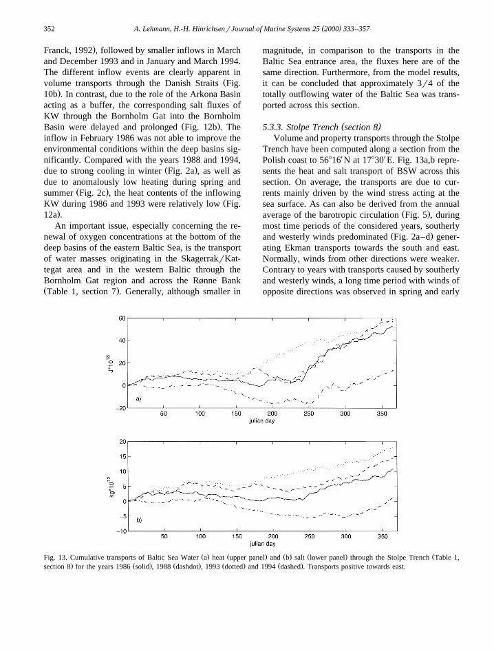
( )5.3.3. Stolpe Trench section 8Volume and property transports through the Stolpe

Trench have been computed along a section from thePolish coast to 56816X N at 17830X E. Fig. 13a,b repre-sents the heat and salt transport of BSW across thissection. On average, the transports are due to cur-rents mainly driven by the wind stress acting at thesea surface. As can also be derived from the annual

Ž .average of the barotropic circulation Fig. 5 , duringmost time periods of the considered years, southerly

Ž .and westerly winds predominated Fig. 2a–d gener-ating Ekman transports towards the south and east.Normally, winds from other directions were weaker.Contrary to years with transports caused by southerlyand westerly winds, a long time period with winds ofopposite directions was observed in spring and early

Ž . Ž . Ž . Ž . ŽFig. 13. Cumulative transports of Baltic Sea Water a heat upper panel and b salt lower panel through the Stolpe Trench Table 1,. Ž . Ž . Ž . Ž .section 8 for the years 1986 solid , 1988 dashdot , 1993 dotted and 1994 dashed . Transports positive towards east.


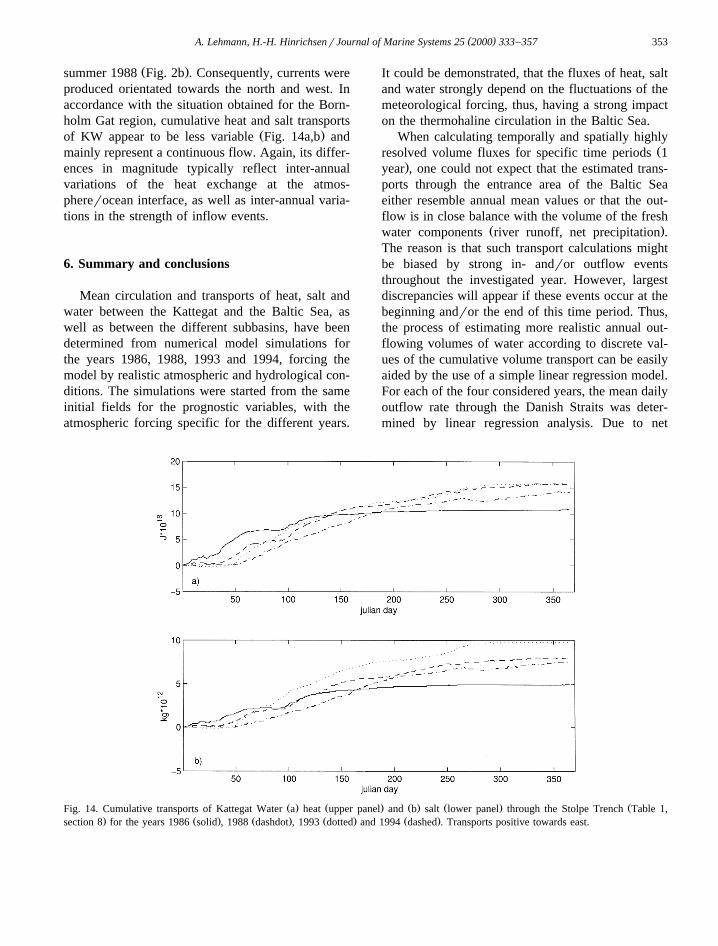
Ž .summer 1988 Fig. 2b . Consequently, currents wereproduced orientated towards the north and west. Inaccordance with the situation obtained for the Born-holm Gat region, cumulative heat and salt transports

Ž .of KW appear to be less variable Fig. 14a,b andmainly represent a continuous flow. Again, its differ-ences in magnitude typically reflect inter-annualvariations of the heat exchange at the atmos-phererocean interface, as well as inter-annual varia-tions in the strength of inflow events.

6. Summary and conclusions

Mean circulation and transports of heat, salt andwater between the Kattegat and the Baltic Sea, aswell as between the different subbasins, have beendetermined from numerical model simulations forthe years 1986, 1988, 1993 and 1994, forcing themodel by realistic atmospheric and hydrological con-ditions. The simulations were started from the sameinitial fields for the prognostic variables, with theatmospheric forcing specific for the different years.

It could be demonstrated, that the fluxes of heat, saltand water strongly depend on the fluctuations of themeteorological forcing, thus, having a strong impacton the thermohaline circulation in the Baltic Sea.

When calculating temporally and spatially highlyŽresolved volume fluxes for specific time periods 1

.year , one could not expect that the estimated trans-ports through the entrance area of the Baltic Seaeither resemble annual mean values or that the out-flow is in close balance with the volume of the fresh

Ž .water components river runoff, net precipitation .The reason is that such transport calculations mightbe biased by strong in- andror outflow eventsthroughout the investigated year. However, largestdiscrepancies will appear if these events occur at thebeginning andror the end of this time period. Thus,the process of estimating more realistic annual out-flowing volumes of water according to discrete val-ues of the cumulative volume transport can be easilyaided by the use of a simple linear regression model.For each of the four considered years, the mean dailyoutflow rate through the Danish Straits was deter-mined by linear regression analysis. Due to net

Ž . Ž . Ž . Ž . ŽFig. 14. Cumulative transports of Kattegat Water a heat upper panel and b salt lower panel through the Stolpe Trench Table 1,. Ž . Ž . Ž . Ž .section 8 for the years 1986 solid , 1988 dashdot , 1993 dotted and 1994 dashed . Transports positive towards east.


Table 2Mean DOR and standard deviations through the Danish Straits

Year DOR STDV3 3Ž . Ž .km rday km rday

1986 1.28 41.01986 1.28 41.01988 1.39 54.41993 2.26 63.61994 1.02 59.1

Ž .precipitation rates according to Omstedt et al. 1997and by the use of annually constant river runoffs, themean daily outflow rate could vary between 1.27 and

1.58 km3rday. The slopes, representing the meanŽ .daily outflow rates DOR and the corresponding

standard deviations of the regression lines for theyears under consideration are summarized in Table2. The DOR for the years 1986 and 1988 are foundto be within the range of the natural variability of thefresh water impact into the Baltic Sea showing rela-tively low standard deviation values. In contrast,

Ž .both remaining years 1993 and 1994 are of differ-ent character. The DOR for these years are farbeyond their expected natural variability range withcorresponding standard deviations suggesting highvariation of transports through the Danish Straits.Furthermore, the outflow rates result from relatively

Fig. 15. Section of salinity differences through the Kattegat, Danish Straits, Arkona Basin, Bornholm Basin and the Stolpe Channel after 3Ž . Ž . Ž . Ž . Ž .months of integration November 1992–January 1993 for a increased river runoff q25% and b decreased river runoff y25% .



strong inflow events at the beginning of each yearpossibly accompanied by high intra-annual changesof volume storage.

It should be noticed that when estimating thewater balance of the Baltic Sea for relatively shorttime scales, the change in volume storage has to beconsidered explicitly. Thus, the differences of thevolume of water according to the temporal change ofthe sea surface elevations between the beginning andthe end of the considered time periods need to becalculated. Besides the precipitation and the evapora-tion rates, the river runoff and the in- and outflowthrough the entrance area, the change of volume

storage is of major importance when closing waterbalances of semi-closed seas such as the Baltic.

To determine the impact of changes of the netfresh water flux on the volume transport and thesalinity flux into the Baltic Sea, sensitivity experi-

Žments for a 3-month simulation period November.1992–January 1993 were carried out varying the

river runoff in the order of its natural variability. Anincrease of the river runoff by 25% resulted in anincreased outflow of BSW masses, and additionally,the wedge-shaped halocline in the Danish Straits wasmoved further to the north, with the consequence ofa pronounced salinity reduction in the Danish Straits,


as well as for the inflowed highly saline wateralready entered the Arkona Basin during the major

Ž .Baltic inflow Fig. 15a . In contrast, the reduction ofriver runoff by the same magnitude led to an in-

Ž .crease of salinity within the same areas Fig. 15b .Ž .An intensified fresh water input q25% resulted in

a decrease of the net transport through the DanishStraits of about 9.4%, whereas a reduction of the

Ž .river runoff y25% yielded an increase of the samevalue. The influence of the variability of the freshwater component on the circulation patterns of theBaltic Sea can be recognized when considering thesalt transports through the Danish Straits: in case ofa reduced fresh water component, the intensifiedvolume transport is accompanied by a cumulativesalt transport of 3.04=1012 kg. In case of an in-crease of river runoff, a transport of 2.07=1012 kgwas obtained. Thus, uncertainties in the net freshwater flux have a strong impact on the volume andsalt fluxes into the Baltic Sea. These uncertaintiesmay be caused either by errors in determining theriver runoff andror the almost unknown precipita-tion and the evaporation rates, which strongly de-pend on the correct simulation of the sea surfacetemperature. These effects, together with uncertain-ties in the numerical model, limit the quantitativedescription of the fluxes involved. However, theorder and the variability of the transports of heat, saltand water are reasonable and may serve as an esti-mation which may be improved in future by furthernumerical, as well as observational, investigations.From the sensitivity study, one can also deduce thatchanges in river runoff or precipitation caused bynatural variability or anthropogenic impact will alsohave an effect on the volume and salt exchange ofthe Baltic Sea with the North Sea.

A full understanding and description of the ther-mohaline circulation and the closing of the energyand water budget of the Baltic Sea will require

Ž .long-term 10–20 years numerical simulations. Forthis kind of numerical investigation, the utilization ofassimilation techniques may become necessary,which additionally increase the requirements oncomputer power. However, less expensive methodssuch as nudging or partial re-initialisation of temper-ature and salinity fields by observations into a cur-

Žrent model run are available e.g. Hinrichsen et al.,.1997 and may be used to improve the simulation of

the thermohaline circulation and its long-term vari-ability.

Acknowledgements

Part of the work was supported by EC MAST-IIIŽ .project ‘‘Baltic Sea System Study BASYS ’’, con-

tract MAS3-CT96-0058.

References

Backhaus, J.O., 1996. Climate-sensitivity of European marginalseas, derived from the interpretation of modelling studies. J.Mar. Syst. 7, 361–382.

Baltic Sea Experiment BALTEX — Initial Implementaion Plan,1995. Int. BALTEX Secretariat Pub. Ser., No. 2, 78 pp.

Bergstrom, S., Carlsson, B., 1994. River runoff to the Baltic Sea:¨Ž .1950–1990. Ambio 23 4–5 , 280–287.

Bock, K.H., 1971. Monatskarten des Salzgehaltes der Ostsee.Erganzungsheft zur Hydrographischen Zeitschrift, Reihe B,¨no. 12.

Bryan, K., 1969. A numerical method for the study of thecirculation of the world ocean. J. Phys. Oceanogr. 15, 1312–1324.

Cox, M.D., 1984. A primitive equation 3-dimensional model ofthe ocean. GFDL Ocean Group Tech. Rep. No. 1, GFDLrPrinceton University.

Ekman, M., Makinen, J., 1996. Mean sea surface topography in¨the Baltic Sea and it’s transition to the North Sea. A geodeticsolution and comparison with oceanographic models. J. Geo-

Ž .phys. Res. 101 C5 , 11993–11999.Haapala, J., Lepparanta, M., 1996. Simulating the Baltic Sea ice¨

season with a coupled ice–ocean model. Tellus 48A, 622–643.Hakansson, B., 1999. On the water and salt exchange in a

frictionally dominated strait — connecting the Baltic Sea withthe North Sea. Cont. Shelf Res., in press.

HELCOM, 1986. Baltic Marine Environment Protection Commis-sion — Helsinki Commission, 1986 Baltic Sea EnvironmentProceedings No. 16, Helsinki, Finland, 174 pp.

Henning, D., 1988. Evaporation, water and heat balance of theBaltic Sea. Estimates of short- and long-term monthly totals.Meteorol. Rundsch. 41, 33–53.

Hibler, W.D. III, 1979. A dynamic thermodynamic sea ice model.J. Phys. Oceanogr. 9, 815–846.

Hinrichsen, H.-H., Lehmann, A., St. John, M., Brugge, B., 1997.¨Modeling the cod larvae drift in the Bornholm Basin in

Ž .summer 1994. Cont. Shelf Res. 17 14 , 1765–1784.Huber, K., Kleine, E., Lass, H.U., Matthaus, W., 1994. The major¨

Baltic inflow in January 1993 — measurements and modellingresults. Dtsch. Hydrogr. Z. 46, 103–114.

Isemer, H.J., Hasse, L., 1987. The Bunker climate atlas of theNorth Atlantic Ocean, Air–Sea Interaction vol. 2 Springer-Verlag, Berlin, 252 pp.

Jacobsen, T.S., 1980. Sea water exchange of the Baltic — mea-


surements and methods. The Belt project. Natl. Agency Envi-ron. Prot., Denmark, 107 pp.

Jerlov, N.G., 1968. Optical Oceanography. Elsevier, Amsterdam,194 pp.

Killworth, P., Stainforth, D., Webbs, D.J., Paterson, S.M., 1991.The development of a free-surface Bryan–Cox–Semtner oceanmodel. J. Phys. Oceanogr. 21, 1333–1348.

Krauss, W., Brugge, B., 1991. Wind-produced water exchange¨between deep basins of the Baltic Sea. J. Phys. Oceanogr. 11,373–384.

Lehmann, A., 1995. A three-dimensional baroclinic eddy-resolv-ing model of the Baltic Sea. Tellus 47, 1013–1031.

Lenz, W., 1971. Monatskarten der Temperatur der Ostsee.Erganzungsheft zur Hydrographischen Zeitschrift, Reihe B,¨no. 11.

Liljebladh, B., Stigebrandt, A., 1996. Observations of the deepwa-Ž .ter flow into the Baltic. J. Geophys. Res. 101 C4 , 8895–8911.

Lisitzin, E., 1974. Sea-level changes. Elsevier Oceanogr. Ser. 8,1–286.

Matthaus, W., Franck, H., 1992. Characteristics of major Baltic¨inflows — a statistical analysis. Cont. Shelf Res. 12, 1375–1400.

Matthaus, W., Lass, H.U., 1995. The recent salt inflow into the¨Baltic Sea. J. Phys. Oceanogr. 25, 280–286.

Mesinger, F., Arakawa, A., 1976. Numerical Methods used inatmospheric models. GARP Publ. Ser. No. 17, Geneva, 64 pp.

Omstedt, A., 1990. A coupled one-dimensional sea–ice–oceanmodel applied to a semi-enclosed basin. Tellus 42A, 568–582.

Omstedt, A., 1996. Response of Baltic Sea ice to seasonal,interannual forcing and climate change. Tellus 48A, 644–662.

Omstedt, A., Rutgersson, A., 2000. Closing the water and heatcycles of the Baltic Sea. Meteorologische Zeitschrift 9, 59–66.

Omstedt, A., Meuller, L., Nyberg, L., 1997. Interannual, seasonal,and regional variations of precipitation and evaporation overthe Baltic Sea. Ambio 26, 484–492.

Parkinson, C.L., Washington, W.M., 1979. A large scale numeri-cal model of sea ice. J. Geophys. Res. 84, 311–337.

Paulsen, E.A., Simpson, J.J., 1977. Irradiance measurements inthe upper ocean. J. Phys. Oceanogr. 7, 952–956.

Schrum, C., 1997. An icerocean model for North and Baltic Sea.¨ Ž .In: Ozsoy, E., Mikaelyan, A. Eds. , Sensitivity to Change:

ŽBlack Sea, Baltic Sea and North Sea Proceedings of theNATO Advanced Research Workshop, Varna, Bulgaria, 14–18

.November, 1995 . Kluwer Academic Publishing, Netherlands,pp. 311–325.

Semtner, A.J., 1974. A general circulation model for the WorldOcean. UCLA Dept. of Meteorology Tech. Rep. No. 8, 99 pp.

Sjoberg, B., 1992. Sea and Coast. National Atlas of Sweden. SNA¨Publishing, SMHI, Norrkoping, 128 pp.¨

Stigebrandt, A., 1987. A model for the vertical circulation of theBaltic deep water. J. Phys. Oceanogr. 17, 1772–1785.

Stossel, A., Owens, W.B., 1992. The Hamburg sea–ice model.¨DKRZ Techn. Rep. No. 3.

Zhang, Z., Lepparanta, M., 1995. Modeling the influence of ice on¨sea level variations in the Baltic Sea. Geophysica 31, 31–45.

Zillman, J.W., 1972. A study of some aspects of the radiation andheat budgets of the southern hemisphere oceans. Meteorol.Stud. Rep. 26, Bur. of Meteorol., Dept. of the Interios, Can-berra, A.C.T.

Documents

On the thermohaline variability of the Baltic Sea