On Time-series Topological Data Analysis: New Data and Opportunities

Lee M. Seversky

Air Force Research Laboratory

Lee.Seversky@us.af.mil

Shelby Davis

Black River Systems

Davis@brsc.com

Matthew Berger

Air Force Research Laboratory

Matthew.Berger.1@us.af.mil

Abstract

This work introduces a new dataset and framework for

the exploration of topological data analysis (TDA) tech-

niques applied to time-series data. We examine the end-to-

end TDA processing pipeline for persistent homology ap-

plied to time-delay embeddings of time series – embeddings

that capture the underlying system dynamics from which

time series data is acquired. In particular, we consider sta-

bility with respect to time series length, the approximation

accuracy of sparse filtration methods, and the discriminat-

ing ability of persistence diagrams as a feature for learn-

ing. We explore these properties across a wide range of

time-series datasets spanning multiple domains for single

source multi-segment signals as well as multi-source sin-

gle segment signals. Our analysis and dataset captures the

entire TDA processing pipeline and includes time-delay em-

beddings, persistence diagrams, topological distance mea-

sures, as well as kernels for similarity learning and classifi-

cation tasks for a broad set of time-series data sources. We

outline the TDA framework and rationale behind the dataset

and provide insights into the role of TDA for time-series

analysis as well as opportunities for new work.

1. Introduction

Topological data analysis (TDA) has shown to be a pow-

erful tool for analyzing complex data sets. Techniques such

as persistent homology [11] have led to new insights and

methods for exploring the topological properties and shape

of data. TDA techniques have been applied to diverse prob-

lem sets including 3D shape matching [4, 26], recurrent

system modeling [30], and periodicity detection [25]. Of

recent interest is the exploration and application of TDA

to time-delay embeddings of time series for the modeling

and classification of dynamical systems and time-varying

events [33, 24, 34].

Time-delay embeddings have primarily been considered

in the context of analyzing dynamical systems [31], where

a time-delay embedding of time-series data can be used

to recover the underlying dynamics of a system. As a re-

sult, the time-delay embedding model has been used by a

number of techniques including chaotic attractors [2] and

more recently considered jointly with TDA, for example,

in analyzing human speech [3] and classification [24, 12].

While TDA techniques show promise as a powerful de-

scriptor for modeling and understanding time-series, there

currently does not exist a comprehensive study character-

izing these techniques in the context of broader types of

time-series sources that are currently being considered by

the larger research community.

This work is motivated by two recent and growing trends

in TDA. First, with the development of more computation-

ally efficient TDA techniques [29, 9, 16], it is now possible

to consider larger and more realistic datasets. For exam-

ple, the recently introduced sparse filtration technique [29]

enables linear-size approximations of the Vietoris-Rips fil-

tration, which is a core component for many TDA tasks,

and enables the efficient construction of persistence dia-

grams. Similarly, the recent geometry-aware technique

[16] for computing Wasserstein and Bottleneck distances

on persistence diagrams provides a computationally effi-

cient means for measuring similarity across persistence di-

agrams. With these advancements come new opportunities

in TDA and time-series applications, such as change point

detection [15], motif finding [18], and classification [3].

Second, there has been a growing trend in exploring

how topological information can be used to form geometry

and topology enriched representations for machine learn-

ing [22, 21]. While techniques for building topological

features have been developed, it has been only recent that

topology has been considered in the context of the large

class of kernel-based learning techniques. In [26], a multi-

scale kernel for persistence diagrams is introduced that de-

fines a persistence scale space kernel, providing the connec-

tion between persistence diagrams and widely-used kernel

based techniques, such as SVM and PCA.

With these new opportunities in TDA come new chal-

lenges. To date, there does not exist a comprehensive topo-

logical dataset targeted to both practitioners and researchers

alike for exploring topological properties and performance

of TDA techniques against well-studied time-varying data

1 59

sets. To address this gap, this work introduces a new time-

series topology dataset, TS-TOP and a framework for cap-

turing the end-to-end TDA processing and data pipeline.

We discuss the processing pipeline and new dataset and ex-

plore the sensitivity and applicability of TDA methods for

characterizing complex time-varying events and dynamics.

The goal of the dataset and framework is to identify new

opportunities for applying TDA to new domains and make

accessible datasets and advanced topological techniques to

researchers outside the topology community. We hope that

this work can help to further development of efficient com-

putational tools and new TDA based learning applications.

2. Time-series TDA Processing Pipeline

In this section, we introduce the main components of our

time-series processing framework that was used to create

the TS-TOP dataset. Different from existing publicly avail-

able computational frameworks targeted for general TDA

[32, 20, 19], our framework explicitly considers TDA in

the context of time-series analysis, where the focus is on

exploring topological properties with respect to different

delay-embeddings, approximations, and time-series learn-

ing tasks. Our time-series processing pipeline is shown in

Figure 1.

Time-delay Embedding: Following [23, 31] for gen-

eral time-series data and built upon by [25] to explore topo-

logical properties of 1-dimensional time-varying signals,

we construct a time-delay embedding of the input signal.

The embedded signal is then partitioned into segments of a

specified length.

Formally, given a 1-dimensional signal f of length

n, the time-delay embedding of f is the set of

points X = (xt, xt+1, . . . , xt+(n−m)), where xt =(ft, ft+1, . . . , ft+m) and xt ∈ R

m−1. While it is possi-

ble to examine the topology using all of X , for time-series

it is of interest to examine the embedded points as a func-

tion of time. Therefore, for single-source continuous sig-

nals, we partition X into a set of segments {S}j , such

that sj = (xj , x(j+1), . . . , x(j+k)), where k is the segment

length and j is the segment start. For multi-source signals,

we represent each signal source as one segment, such that

the point cloud X comprises a single segment. Additional

details of the dataset types can be found in Section 3.

Persistence Diagrams: Given the segments, we wish to

explore the topology of each segment through the analysis

of the embedded point cloud and its persistence diagram.

Persistence diagrams [10] provide a concise description of

the topological changes over all scales of the data. This

multiple scale viewpoint of the data can be realized via per-

sistent homology [10] through a filtration on the data which

captures the growth, birth, and death of different topologi-

cal features across dimensions (e.g. components, tunnels,

voids). From this filtration, the birth and death of a k-

dimensional component can be described by a point (a, b)in the persistence diagram of dimension k, where a, b is the

birth and death times respectively. A key challenge asso-

ciated with computing persistence is its dependence on the

filtration size, which grows as O(nk+1) for simplices up to

dimension k. We use the recent sparse Vietoris-Rips filtra-

tion [29] to produce a linear-size filtration, which is then

used in the computation of the persistence diagram via the

standard pairing algorithm [10].

The persistence diagram is comprised of the set of all k-

dimensional birth-death pairs forming a multiset of points in

R2. These pairings capture the topology of the space across

all scales such that a significant topological feature persists

as a function of time [10]. Specifically, we are interested

in exploring the 1-dimensional persistence diagrams, which

provides a concise description of topological 1-dimensional

cycles that may exist in the data. This is particularly infor-

mative, as such cycles can provide insights into periodic and

repetitive patterns often found in time-series data and can

serve as important discriminating descriptors [25]. There-

fore, we focus our efforts on computing and analyzing 1-

dimensional persistence diagrams for the characterization

of periodic and repetitive patterns.

Distance Measures: Given persistence diagrams it is

only natural to want to compare diagrams with respect to

topological similarity. A distance metric for persistence di-

agrams provides a means for relating the topology of data

and more generally the datasets in terms of topological sim-

ilarity and has received much attention [1, 14]. In general

persistence diagrams are stable, where small changes in the

data results in small changes in the diagram [7]. Two com-

mon distance metrics are the Wasserstein and Bottleneck

distances. Wasserstein distance is defined as the sum of

the q-th powers of the distances between points across all

matchings between persistence diagrams. A specialization

of the Wasserstein distance is the bottleneck distance, which

is the Wasserstein distance in the limit as q goes to infinity,

and is the largest distance between two points in the best

matching [10]. In the case of the bottleneck distance it is

stable with respect to perturbations [7]. We use these dis-

tance measures to compute all-segment pairwise distances

across all time-series datasets utilizing recent efficient tech-

niques introduced in [16].

Topological Kernels: A growing area of interest is

the use of topological information for machine learning

tasks. Prior approaches focused on featured-based descrip-

tors built directly from persistence diagrams. For example,

in [22] the persistence diagrams are rasterized as images and

an image-based feature is then derived and used to build

a standard image-based kernel to train an SVM classifier.

Such approaches impose arbitrary representations on top of

the persistence diagram in order to utilize traditional learn-

ing techniques with topology. Alternatively, [17] considers

60

Source Data Segment Selection Time Delay Reconstruction Persistence Diagram

Bottleneck Distance Wasserstein DistanceScale Space Kernel

Window Selection Point Cloud

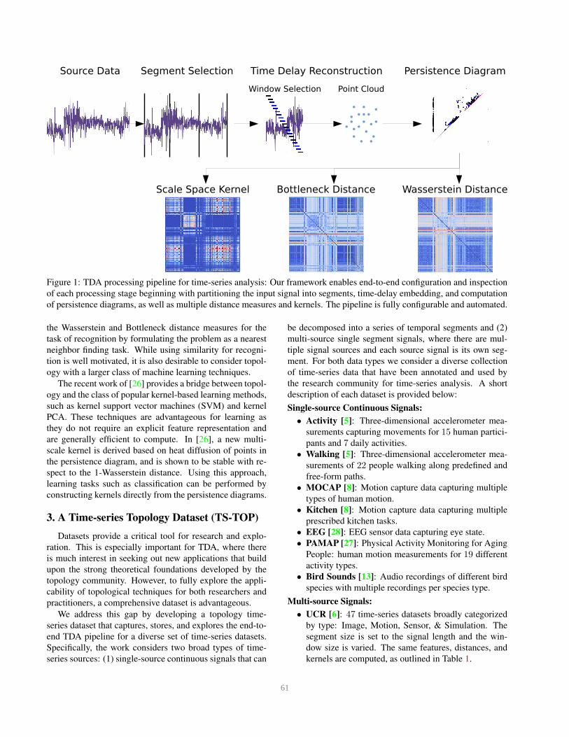
Figure 1: TDA processing pipeline for time-series analysis: Our framework enables end-to-end configuration and inspection

of each processing stage beginning with partitioning the input signal into segments, time-delay embedding, and computation

of persistence diagrams, as well as multiple distance measures and kernels. The pipeline is fully configurable and automated.

the Wasserstein and Bottleneck distance measures for the

task of recognition by formulating the problem as a nearest

neighbor finding task. While using similarity for recogni-

tion is well motivated, it is also desirable to consider topol-

ogy with a larger class of machine learning techniques.

The recent work of [26] provides a bridge between topol-

ogy and the class of popular kernel-based learning methods,

such as kernel support vector machines (SVM) and kernel

PCA. These techniques are advantageous for learning as

they do not require an explicit feature representation and

are generally efficient to compute. In [26], a new multi-

scale kernel is derived based on heat diffusion of points in

the persistence diagram, and is shown to be stable with re-

spect to the 1-Wasserstein distance. Using this approach,

learning tasks such as classification can be performed by

constructing kernels directly from the persistence diagrams.

3. A Time-series Topology Dataset (TS-TOP)

Datasets provide a critical tool for research and explo-

ration. This is especially important for TDA, where there

is much interest in seeking out new applications that build

upon the strong theoretical foundations developed by the

topology community. However, to fully explore the appli-

cability of topological techniques for both researchers and

practitioners, a comprehensive dataset is advantageous.

We address this gap by developing a topology time-

series dataset that captures, stores, and explores the end-to-

end TDA pipeline for a diverse set of time-series datasets.

Specifically, the work considers two broad types of time-

series sources: (1) single-source continuous signals that can

be decomposed into a series of temporal segments and (2)

multi-source single segment signals, where there are mul-

tiple signal sources and each source signal is its own seg-

ment. For both data types we consider a diverse collection

of time-series data that have been annotated and used by

the research community for time-series analysis. A short

description of each dataset is provided below:

Single-source Continuous Signals:

• Activity [5]: Three-dimensional accelerometer mea-

surements capturing movements for 15 human partici-

pants and 7 daily activities.

• Walking [5]: Three-dimensional accelerometer mea-

surements of 22 people walking along predefined and

free-form paths.

• MOCAP [8]: Motion capture data capturing multiple

types of human motion.

• Kitchen [8]: Motion capture data capturing multiple

prescribed kitchen tasks.

• EEG [28]: EEG sensor data capturing eye state.

• PAMAP [27]: Physical Activity Monitoring for Aging

People: human motion measurements for 19 different

activity types.

• Bird Sounds [13]: Audio recordings of different bird

species with multiple recordings per species type.

Multi-source Signals:

• UCR [6]: 47 time-series datasets broadly categorized

by type: Image, Motion, Sensor, & Simulation. The

segment size is set to the signal length and the win-

dow size is varied. The same features, distances, and

kernels are computed, as outlined in Table 1.

61

Dataset Records Dim Classes Seg. Size Win. Size Features Distances Kernel

Activity [5] 1,926,896 3 7 1000, 2000 50,100,150 PD0,1 W,B SSK, RBF

Walking [5] 149,322 3 22 200 15 PD0,1 W,B SSK, RBF

Mocap [8] 225,551* 62 2* 150 15 PD0,1, CI W,B SSK

Kitchen [8] 17,726,895 9 5 1000 120 PD0,1 W,B SSK, RBF

EEG Eye [28] 14,980 16 2 300 20 PD0,1 W,B SSK, RBF

PAMAP [27] 2,872,533 52 19 1000 20,30,40,50 PD0,1 W,B SSK, RBF

Bird Sounds [13] 24,050,377 1 16 800 15,30,45 PD0,1 W,B SSK, RBF

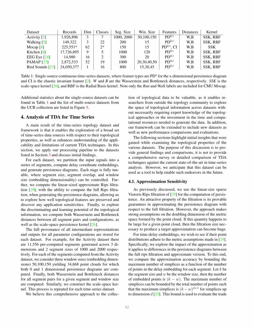
Table 1: Single-source continuous time-series datasets, where feature types are PDx for the x-dimensional persistence diagram

and CI is the chaotic invariant feature [2]. W and B are the Wasserstein and Bottleneck distances, respectively. SSK is the

scale-space kernel [26], and RBF is the Radial Basis kernel. Note only the Run and Walk labels are included for CMU Mocap.

Additional statistics about the single-source datasets can be

found in Table 1 and the list of multi-source datasets from

the UCR collection are listed in Figure 5.

4. Analysis of TDA for Time Series

A main result of the time-series topology dataset and

framework is that it enables the exploration of a broad set

of time-series data sources with respect to their topological

properties, as well as enhances understanding of the appli-

cability and limitations of current TDA techniques. In this

section, we apply our processing pipeline to the datasets

listed in Section 3 and discuss initial findings.

For each dataset, we partition the input signals into a

series of segments, compute delay coordinate embeddings,

and generate persistence diagrams. Each stage is fully tun-

able, where segment size, segment overlap, and window

size (embedding dimensionality) can be controlled. Fur-

ther, we compute the linear-sized approximate Rips filtra-

tion [29], with the ability to compute the full Rips filtra-

tion, when generating the persistence diagrams, allowing us

to explore how well topological features are preserved and

discover any application sensitivities. Finally, to explore

the discriminating and learning potential of the topological

information, we compute both Wasserstein and Bottleneck

distances between all segment pairs and configurations, as

well as the scale-space persistence kernel [26].

The full provenance of all intermediate representations

and outputs for all parameter configurations are stored for

each dataset. For example, for the Activity dataset there

are 11,556 pre-computed segments generated across 3 di-

mensions and 2 segment sizes of 1000 and 2000 respec-

tively. For each of the segments computed from the Activity

dataset, we consider three window sizes (embedding dimen-

sions) 50,100,150 yielding 34,668 point clouds for which

both 0 and 1 dimensional persistence diagrams are com-

puted. Finally, both Wasserstein and Bottleneck distances

for all segment pairs for a given segment and window size

are computed. Similarly, we construct the scale-space ker-

nel. This process is repeated for each time-series dataset.

We believe this comprehensive approach to the collec-

tion of topological data to be valuable, as it enables re-

searchers from outside the topology community to explore

the space of topological information across datasets with-

out necessarily requiring expert knowledge of the topolog-

ical approaches or the investment in the time and compu-

tational resources needed to generate the data. In addition,

our framework can be extended to include new datasets as

well as new performance comparisons and evaluations.

The following sections highlight initial insights that were

gained while examining the topological properties of the

various datasets. The purpose of this discussion is to pro-

vide general findings and comparisons, it is not to provide

a comprehensive survey or detailed comparison of TDA

techniques against the current state-of-the-art in time-series

analysis. However, we anticipate that this dataset can be

used as a tool to help enable such endeavors in the future.

4.1. Approximation Sensitivity

As previously discussed, we use the linear-size sparse

Vietoris Rips filtration of [29] for the computation of persis-

tence. An attractive property of the filtration is its provable

guarantees in approximating the persistence diagram with

respect to the full filtration. However, the approach makes

strong assumptions on the doubling dimension of the metric

space formed by the point cloud. If this quantity happens to

be large for a given point cloud, then the filtration size nec-

essary to produce a target approximation can become huge.

For time-delay embeddings, we wish to see if their point

distributions adhere to the metric assumptions made in [29].

Specifically, we explore the impact of the approximation as

it applies to differences in the persistence diagrams between

the full rips filtration and approximate version. To this end,

we compare the approximation accuracy by bounding the

maximum number of simplices as a function of the number

of points in the delay embedding for each segment. Let k be

the segment size and w be the window size, then the number

of embedded points is (k − w). The maximum number of

simplices can be bounded by the total number of points such

that the maximum simplices is (k−w)d+1 for simplices up

to dimension d [29]. This bound is used to evaluate the trade

62

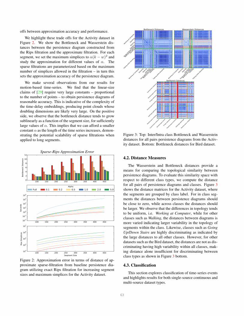
offs between approximation accuracy and performance.

We highlight these trade offs for the Activity dataset in

Figure 2. We show the Bottleneck and Wasserstein dis-

tances between the persistence diagram constructed from

the Rips filtration and the approximate filtration. For each

segment, we set the maximum simplices to α(k − w)2 and

study the approximation for different values of α. The

sparse filtrations are parameterized based on the maximum

number of simplices allowed in the filtration – in turn this

sets the approximation accuracy of the persistence diagram.

We make several observations from our results for

motion-based time-series. We find that the linear-size

claims of [29] require very large constants – proportional

to the number of points – to obtain persistence diagrams of

reasonable accuracy. This is indicative of the complexity of

the time-delay embeddings, producing point clouds whose

doubling dimensions are likely very large. On the positive

side, we observe that the bottleneck distance tends to grow

sublinearly as a function of the segment size, for sufficiently

large values of α. This implies that we can afford a smaller

constant α as the length of the time series increases, demon-

strating the potential scalability of sparse filtrations when

applied to long segments.

Sparse-Rips Approximation Error

100 150 200 250 300 350 400 4500

2

4

6

8

10

12

Bott

leneck D

ista

nce

100 150 200 250 300 350 400 45010

-2

10-1

100

101

102

103

104

Seconds

Alpha

Full 0.1 0.2 0.5 1.0 2.0 5.0

100 150 200 250 300 350 400 450

Segment Size

103

104

105

106

107

Max S

implices

Figure 2: Approximation error in terms of distance of ap-

proximate sparse-filtration from baseline persistence dia-

gram utilizing exact Rips filtration for increasing segment

sizes and maximum simplices for the Activity dataset.

Wor

king

at Com

pute

r

Stan

ding

Walking

Stan

ding

Going

Up/

Dow

n St

airs

Stan

ding

Walking

and

Talking

Talkin

g whi

le S

tand

ing

Wor

king

at Com

pute

r

Stan

ding

Walking

Stan

ding

Going

Up/

Dow

n St

airs

Stan

ding

Walking

and

Talking

Talkin

g whi

le S

tand

ing

Bottleneck Distances Wasserstein Distances

Wor

king

at Com

pute

r

Stan

ding

Walking

Stan

ding

Going

Up/

Dow

n St

airs

Stan

ding

Walking

and

Talking

Talkin

g whi

le S

tand

ing

Cya

noco

rax-

violac

eus

Den

droc

opos

-min

or

Trin

ga-n

ebul

aria

Phyllosc

opus

-tro

chilu

s

Gallin

ago-

gallina

go

Phyllosc

opus

-collybi

ta

Cya

noco

rax-

violac

eus

Den

droc

opos

-min

or

Trin

ga-n

ebul

aria

Phyllosc

opus

-tro

chilu

s

Gallin

ago-

gallina

go

Phyllosc

opus

-collybi

ta

Bottleneck Distances

Figure 3: Top: Inter/Intra class Bottleneck and Wasserstein

distances for all pairs persistence diagrams from the Activ-

ity dataset. Bottom: Bottleneck distances for Bird dataset.

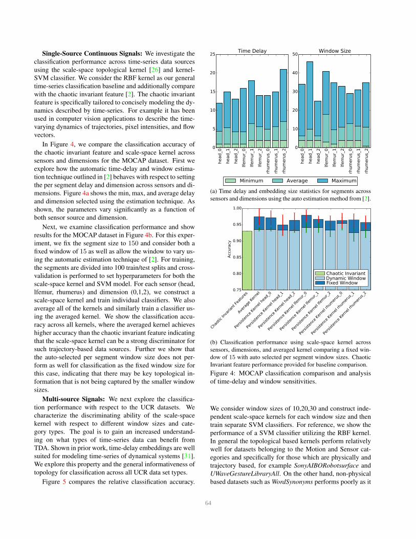
4.2. Distance Measures

The Wasserstein and Bottleneck distances provide a

means for comparing the topological similarity between

persistence diagrams. To evaluate this similarity space with

respect to different class types, we compute the distance

for all pairs of persistence diagrams and classes. Figure 3

shows the distance matrices for the Activity dataset, where

the segments are grouped by class label. For in class seg-

ments the distances between persistence diagrams should

be close to zero, while across classes the distances should

be larger. We observe that the differences in topology tends

to be uniform, i.e. Working at Computer, while for other

classes such as Walking, the distances between diagrams is

more varied indicating larger variability in the topology of

segments within the class. Likewise, classes such as Going

Up/Down Stairs are highly discriminating as indicated by

the large distances to all other classes. However, for other

datasets such as the Bird dataset, the distances are not as dis-

criminating having high variability within all classes, mak-

ing distance alone insufficient for discriminating between

class types as shown in Figure 3 bottom.

4.3. Classification

This section explores classification of time-series events

and highlights results for both single-source continuous and

multi-source dataset types.

63

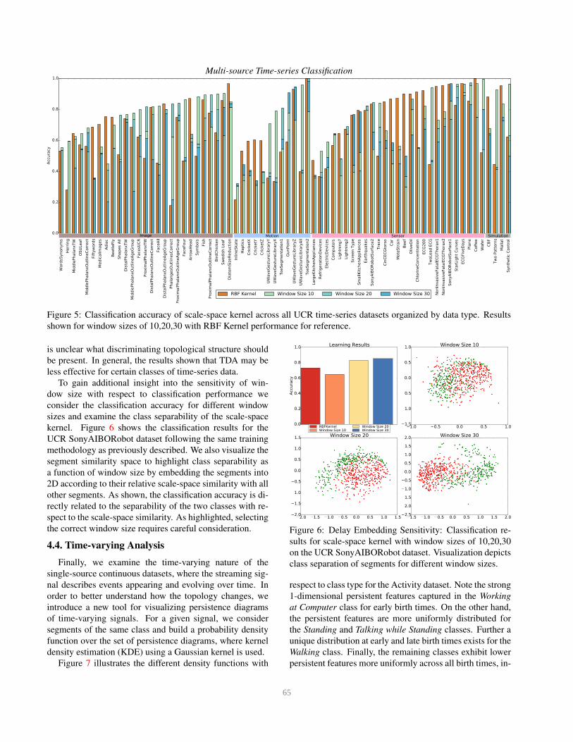
Single-Source Continuous Signals: We investigate the

classification performance across time-series data sources

using the scale-space topological kernel [26] and kernel-

SVM classifier. We consider the RBF kernel as our general

time-series classification baseline and additionally compare

with the chaotic invariant feature [2]. The chaotic invariant

feature is specifically tailored to concisely modeling the dy-

namics described by time-series. For example it has been

used in computer vision applications to describe the time-

varying dynamics of trajectories, pixel intensities, and flow

vectors.

In Figure 4, we compare the classification accuracy of

the chaotic invariant feature and scale-space kernel across

sensors and dimensions for the MOCAP dataset. First we

explore how the automatic time-delay and window estima-

tion technique outlined in [2] behaves with respect to setting

the per segment delay and dimension across sensors and di-

mensions. Figure 4a shows the min, max, and average delay

and dimension selected using the estimation technique. As

shown, the parameters vary significantly as a function of

both sensor source and dimension.

Next, we examine classification performance and show

results for the MOCAP dataset in Figure 4b. For this exper-

iment, we fix the segment size to 150 and consider both a

fixed window of 15 as well as allow the window to vary us-

ing the automatic estimation technique of [2]. For training,

the segments are divided into 100 train/test splits and cross-

validation is performed to set hyperparameters for both the

scale-space kernel and SVM model. For each sensor (head,

lfemur, rhumerus) and dimension (0,1,2), we construct a

scale-space kernel and train individual classifiers. We also

average all of the kernels and similarly train a classifier us-

ing the averaged kernel. We show the classification accu-

racy across all kernels, where the averaged kernel achieves

higher accuracy than the chaotic invariant feature indicating

that the scale-space kernel can be a strong discriminator for

such trajectory-based data sources. Further we show that

the auto-selected per segment window size does not per-

form as well for classification as the fixed window size for

this case, indicating that there may be key topological in-

formation that is not being captured by the smaller window

sizes.

Multi-source Signals: We next explore the classifica-

tion performance with respect to the UCR datasets. We

characterize the discriminating ability of the scale-space

kernel with respect to different window sizes and cate-

gory types. The goal is to gain an increased understand-

ing on what types of time-series data can benefit from

TDA. Shown in prior work, time-delay embeddings are well

suited for modeling time-series of dynamical systems [31].

We explore this property and the general informativeness of

topology for classification across all UCR data set types.

Figure 5 compares the relative classification accuracy.

Minimum Average Maximum

head_0

head_1

head_2

lfem

ur_

0

lfem

ur_

1

lfem

ur_

2

rhum

eru

s_0

rhum

eru

s_1

rhum

eru

s_20

5

10

15

20

25Time Delay

head_0

head_1

head_2

lfem

ur_

0

lfem

ur_

1

lfem

ur_

2

rhum

eru

s_0

rhum

eru

s_1

rhum

eru

s_20

10

20

30

40

50Window Size

(a) Time delay and embedding size statistics for segments across

sensors and dimensions using the auto estimation method from [2].

Chaot

ic In

varia

nt Fea

ture

s

Avera

ge K

erne

l

Pers

iste

nce

Kern

el h

ead_

0

Pers

iste

nce

Kern

el h

ead_

1

Pers

iste

nce

Kern

el h

ead_

2

Pers

iste

nce

Kern

el lf

emur

_0

Pers

iste

nce

Kern

el lf

emur

_1

Pers

iste

nce

Kern

el lf

emur

_2

Pers

iste

nce

Kern

el rhu

mer

us_0

Pers

iste

nce

Kern

el rhu

mer

us_1

Pers

iste

nce

Kern

el rhu

mer

us_2

0.75

0.80

0.85

0.90

0.95

1.00

Accura

cy

Chaotic InvariantDynamic WindowFixed Window

(b) Classification performance using scale-space kernel across

sensors, dimensions, and averaged kernel comparing a fixed win-

dow of 15 with auto selected per segment window sizes. Chaotic

Invariant feature performance provided for baseline comparison.

Figure 4: MOCAP classification comparison and analysis

of time-delay and window sensitivities.

We consider window sizes of 10,20,30 and construct inde-

pendent scale-space kernels for each window size and then

train separate SVM classifiers. For reference, we show the

performance of a SVM classifier utilizing the RBF kernel.

In general the topological based kernels perform relatively

well for datasets belonging to the Motion and Sensor cat-

egories and specifically for those which are physically and

trajectory based, for example SonyAIBORobotsurface and

UWaveGestureLibraryAll. On the other hand, non-physical

based datasets such as WordSynonyms performs poorly as it

64

Multi-source Time-series Classification

Word

sSynonym

s

Herr

ing

Mid

dle

Phala

nxTW

OSU

Leaf

Mid

dle

Phala

nxO

utl

ineC

orr

ect

Fifty

word

s

Medic

alIm

ages

Adia

c

Beetl

eFly

Shapes A

ll

Dis

talP

hala

nxTW

Mid

dle

Phala

nxO

utl

ineA

geG

roup

FacesU

CR

Pro

xim

alP

hala

nxTW

Dis

talP

hala

nxO

utl

ineC

orr

ect

FaceA

ll

Dis

talP

hala

nxO

utl

ineA

geG

roup

Phala

ngesO

utl

inesC

orr

ect

Pro

xim

alP

hala

nxO

utl

ineA

geG

roup

FaceFour

Arr

ow

Head

Sym

bols

Fis

h

Pro

xim

alP

hala

nxO

utl

ineC

orr

ect

Bir

dC

hic

ken

Sw

edis

h L

eaf

Dia

tom

Siz

eR

educti

on

InlineSkate

Hapti

cs

Cri

cketX

Cri

cketY

Cri

cketZ

UW

aveG

estu

reLib

rary

Y

UW

aveG

estu

reLib

rary

X

ToeSegm

enta

tion1

GunPoin

t

UW

aveG

estu

reLib

rary

Z

UW

aveG

estu

reLib

rary

All

ToeSegm

enta

tion2

Larg

eK

itchenA

ppliances

Refr

igera

tionD

evic

es

Ele

ctr

icD

evic

es

Com

pute

rs

Lig

htn

ing7

Lig

htn

ing2

Scre

en T

ype

Sm

allK

itchenA

ppliances

Eart

hquakes

SonyA

IBO

RobotS

urf

ace2

Tra

ce

Cin

CEC

Gto

rso

Car

Mote

Str

ain

Beef

OliveO

il

Chlo

rineC

oncentr

ati

on

EC

G2

00

Tw

oLead E

CG

NonIn

vasiv

eFata

lEC

GThora

x1

NonIn

vasiv

eFata

lEC

GThora

x2

SonyA

IBO

RobotS

urf

ace1

Sta

rLig

ht

Curv

es

EC

GFiv

eD

ays

Pla

ne

Coff

ee

Wafe

r

CB

F

Tw

o P

att

ern

s

Mallat

Synth

eti

c C

ontr

ol

0.0

0.2

0.4

0.6

0.8

1.0

Accura

cy

RBF Kernel Window Size 10 Window Size 20 Window Size 30

Image Motion Sensor Simulation

Figure 5: Classification accuracy of scale-space kernel across all UCR time-series datasets organized by data type. Results

shown for window sizes of 10,20,30 with RBF Kernel performance for reference.

is unclear what discriminating topological structure should

be present. In general, the results shown that TDA may be

less effective for certain classes of time-series data.

To gain additional insight into the sensitivity of win-

dow size with respect to classification performance we

consider the classification accuracy for different window

sizes and examine the class separability of the scale-space

kernel. Figure 6 shows the classification results for the

UCR SonyAIBORobot dataset following the same training

methodology as previously described. We also visualize the

segment similarity space to highlight class separability as

a function of window size by embedding the segments into

2D according to their relative scale-space similarity with all

other segments. As shown, the classification accuracy is di-

rectly related to the separability of the two classes with re-

spect to the scale-space similarity. As highlighted, selecting

the correct window size requires careful consideration.

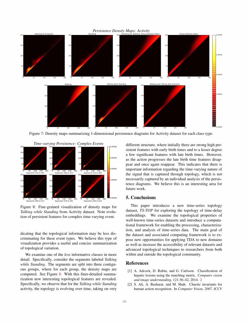
4.4. Time­varying Analysis

Finally, we examine the time-varying nature of the

single-source continuous datasets, where the streaming sig-

nal describes events appearing and evolving over time. In

order to better understand how the topology changes, we

introduce a new tool for visualizing persistence diagrams

of time-varying signals. For a given signal, we consider

segments of the same class and build a probability density

function over the set of persistence diagrams, where kernel

density estimation (KDE) using a Gaussian kernel is used.

Figure 7 illustrates the different density functions with

0.0

0.2

0.4

0.6

0.8

1.0

Accura

cy

Learning Results

RBFKernelWindow Size 10

Window Size 20Window Size 30

1.0 0.5 0.0 0.5 1.01.5

1.0

0.5

0.0

0.5

1.0Window Size 10

2.0 1.5 1.0 0.5 0.0 0.5 1.0 1.52.0

1.5

1.0

0.5

0.0

0.5

1.0

1.5Window Size 20

1.5 1.0 0.5 0.0 0.5 1.0 1.5 2.02.5

2.0

1.5

1.0

0.5

0.0

0.5

1.0

1.5

2.0Window Size 30

Figure 6: Delay Embedding Sensitivity: Classification re-

sults for scale-space kernel with window sizes of 10,20,30

on the UCR SonyAIBORobot dataset. Visualization depicts

class separation of segments for different window sizes.

respect to class type for the Activity dataset. Note the strong

1-dimensional persistent features captured in the Working

at Computer class for early birth times. On the other hand,

the persistent features are more uniformly distributed for

the Standing and Talking while Standing classes. Further a

unique distribution at early and late birth times exists for the

Walking class. Finally, the remaining classes exhibit lower

persistent features more uniformly across all birth times, in-

65

Persistence Density Maps: Activity

0 50 100 150 2000

50

100

150

200Working at Computer

0 50 100 150 2000

50

100

150

200Standing

0 50 100 150 2000

50

100

150

200Standing Up, Walking, Going Up\Down Stairs

0 50 100 150 2000

50

100

150

200Going Up\Down Stairs

0 50 100 150 2000

50

100

150

200Walking

0 50 100 150 2000

50

100

150

200Talking while Standing

0 50 100 150 2000

50

100

150

200Walking and Talking with Someone

0.00000

0.00009

0.00094

0.00938

0.09384

Figure 7: Density maps summarizing 1-dimensional persistence diagrams for Activity dataset for each class type.

Time-varying Persistence: Complex Events

0 50 100 150 200

Segments 316 to 365

0

50

100

150

200

0 50 100 150 200

Segments 366 to 415

0

50

100

150

200

0 50 100 150 200

Segments 416 to 465

0

50

100

150

200

0.00000

0.00009

0.00094

0.00938

0.09384

0 50 100 150 200

Segments 466 to 515

0

50

100

150

200

0 50 100 150 200

Segments 516 to 565

0

50

100

150

200

0 50 100 150 200

Segments 566 to 615

0

50

100

150

200

Figure 8: Fine-grained visualization of density maps for

Talking while Standing from Activity dataset. Note evolu-

tion of persistent features for complex time-varying event.

dicating that the topological information may be less dis-

criminating for these event types. We believe this type of

visualization provides a useful and concise summarization

of topological variation.

We examine one of the less informative classes in more

detail. Specifically, consider the segments labeled Talking

while Standing. The segments are split into three contigu-

ous groups, where for each group, the density maps are

computed. See Figure 8. With this finer-detailed summa-

rization new interesting topological features are revealed.

Specifically, we observe that for the Talking while Standing

activity, the topology is evolving over time, taking on very

different structure, where initially there are strong high per-

sistent features with early birth times and to a lesser degree

a few significant features with late birth times. However,

as the action progresses the late birth time features disap-

pear and once again reappear. This indicates that there is

important information regarding the time-varying nature of

the signal that is captured through topology, which is not

necessarily captured by an individual analysis of the persis-

tence diagrams. We believe this is an interesting area for

future work.

5. Conclusions

This paper introduces a new time-series topology

dataset, TS-TOP for exploring the topology of time-delay

embeddings. We examine the topological properties of

well-known time-series datasets and introduce a computa-

tional framework for enabling the processing, characteriza-

tion, and analysis of time-series data. The main goal of

the dataset and associated computing framework is to ex-

pose new opportunities for applying TDA to new domains

as well as increase the accessibility of relevant datasets and

advanced topological techniques to researchers from both

within and outside the topological community.

References

[1] A. Adcock, D. Rubin, and G. Carlsson. Classification of

hepatic lesions using the matching metric. Computer vision

and image understanding, 121:36–42, 2014. 2

[2] S. Ali, A. Basharat, and M. Shah. Chaotic invariants for

human action recognition. In Computer Vision, 2007. ICCV

66

2007. IEEE 11th International Conference on, pages 1–8.

IEEE, 2007. 1, 4, 6

[3] K. A. Brown and K. P. Knudson. Nonlinear statistics of hu-

man speech data. International Journal of Bifurcation and

Chaos, 19(07):2307–2319, 2009. 1

[4] M. Carriere, S. Y. Oudot, and M. Ovsjanikov. Stable topolog-

ical signatures for points on 3d shapes. In Computer Graph-

ics Forum, volume 34, pages 1–12. Wiley Online Library,

2015. 1

[5] P. Casale, O. Pujol, and P. Radeva. Personalization and user

verification in wearable systems using biometric walking

patterns. Personal and Ubiquitous Computing, 16(5):563–

580, 2012. 3, 4

[6] Y. Chen, E. Keogh, B. Hu, N. Begum, A. Bagnall,

A. Mueen, and G. Batista. The ucr time series classifica-

tion archive, July 2015. www.cs.ucr.edu/˜eamonn/

time_series_data/. 3

[7] D. Cohen-Steiner, H. Edelsbrunner, and J. Harer. Stability of

persistence diagrams. Discrete & Computational Geometry,

37(1):103–120, 2007. 2

[8] F. De la Torre, J. Hodgins, A. Bargteil, X. Martin, J. Macey,

A. Collado, and P. Beltran. Guide to the carnegie mellon uni-

versity multimodal activity (cmu-mmac) database. Robotics

Institute, page 135, 2008. 3, 4

[9] T. K. Dey, F. Fan, and Y. Wang. Computing topological per-

sistence for simplicial maps. In Proceedings of the thirtieth

annual symposium on Computational geometry, page 345.

ACM, 2014. 1

[10] H. Edelsbrunner and J. Harer. Computational topology: an

introduction. American Mathematical Soc., 2010. 2

[11] H. Edelsbrunner, D. Letscher, and A. Zomorodian. Topolog-

ical persistence and simplification. Discrete and Computa-

tional Geometry, 28(4):511–533, 2002. 1

[12] S. Emrani, T. Gentimis, and H. Krim. Persistent homology

of delay embeddings and its application to wheeze detection.

Signal Processing Letters, IEEE, 21(4):459–463, 2014. 1

[13] H. Goeau, H. Glotin, W.-P. Vellinga, R. Planque, A. Rauber,

and A. Joly. Lifeclef bird identification task 2014. In

CLEF2014, 2014. 3, 4

[14] C. Gu, L. Guibas, and M. Kerber. Topology-driven trajectory

synthesis with an example on retinal cell motions. In Algo-

rithms in Bioinformatics, pages 326–339. Springer, 2014. 2

[15] V. Guralnik and J. Srivastava. Event detection from time

series data. In Proceedings of the fifth ACM international

conference on Knowledge discovery and data mining, pages

33–42. ACM, 1999. 1

[16] M. Kerber, D. Morozov, and A. Nigmetov. Geometry

helps to compare persistence diagrams. In Proceedings of

the Workshop on Algorithm Engineering and Experiments

(ALENEX), 2016. 1, 2

[17] C. Li, M. Ovsjanikov, and F. Chazal. Persistence-based

structural recognition. In Proceedings of the IEEE Con-

ference on Computer Vision and Pattern Recognition, pages

1995–2002, 2014. 2

[18] J. L. E. K. S. Lonardi and P. Patel. Finding motifs in time se-

ries. In Proc. of the 2nd Workshop on Temporal Data Mining,

pages 53–68, 2002. 1

[19] D. Morozov. Dionysus library for computing persis-

tent homology. Software available at http://www. mrzv.

org/software/dionysus, 2012. 2

[20] V. Nanda. Perseus: the persistent homology soft-

ware. Software available at http://www. sas. upenn. edu/˜

vnanda/perseus, 2012. 2

[21] L. Oudre, J. Jakubowicz, P. Bianchi, and C. Simon. Clas-

sification of periodic activities using the wasserstein dis-

tance. Biomedical Engineering, IEEE Transactions on,

59(6):1610–1619, 2012. 1

[22] D. Pachauri, C. Hinrichs, M. K. Chung, S. C. Johnson, and

V. Singh. Topology-based kernels with application to in-

ference problems in alzheimer’s disease. Medical Imaging,

IEEE Transactions on, 30(10):1760–1770, 2011. 1, 2

[23] N. H. Packard, J. P. Crutchfield, J. D. Farmer, and R. S.

Shaw. Geometry from a time series. Physical Review Letters,

45(9):712, 1980. 2

[24] J. A. Perea, A. Deckard, S. B. Haase, and J. Harer. Sw1pers:

Sliding windows and 1-persistence scoring; discovering pe-

riodicity in gene expression time series data. BMC bioinfor-

matics, 16(1):257, 2015. 1

[25] J. A. Perea and J. Harer. Sliding windows and persistence:

An application of topological methods to signal analysis.

Foundations of Computational Mathematics, 15(3):799–838,

2015. 1, 2

[26] J. Reininghaus, S. Huber, U. Bauer, and R. Kwitt. A stable

multi-scale kernel for topological machine learning. In Pro-

ceedings of the IEEE Conference on Computer Vision and

Pattern Recognition, pages 4741–4748, 2015. 1, 3, 4, 6

[27] A. Reiss and D. Stricker. Introducing a new benchmarked

dataset for activity monitoring. In Wearable Computers

(ISWC), 2012 16th International Symposium on, pages 108–

109. IEEE, 2012. 3, 4

[28] O. Rosler and D. Suendermann. A first step towards eye state

prediction using eeg. In AIHLS 2013, International Confer-

ence on Applied Informatics for Health and Life Sciences,

Istanbul, Turkey, September 2013. AIHLS. 3, 4

[29] D. R. Sheehy. Linear-size approximations to the vietoris–rips

filtration. Discrete & Computational Geometry, 49(4):778–

796, 2013. 1, 2, 4, 5

[30] P. Skraba, V. de Silva, and M. Vejdemo-Johansson. Topologi-

cal analysis of recurrent systems. In NIPS 2012 Workshop on

Algebraic Topology and Machine Learning, December 8th,

Lake Tahoe, Nevada, pages 1–5, 2012. 1

[31] F. Takens. Detecting strange attractors in turbulence.

Springer, 1981. 1, 2, 6

[32] A. Tausz, M. Vejdemo-Johansson, and H. Adams. Javaplex:

A research software package for persistent (co) homol-

ogy. Software available at http://code. google. com/javaplex,

2011. 2

[33] C. M. Topaz, L. Ziegelmeier, and T. Halverson. Topological

data analysis of biological aggregation models. PloS one,

10(5), 2015. 1

[34] V. Venkataraman, K. N. Ramamurthy, and P. Turaga. Per-

sistent homology of attractors for action recognition. arXiv

preprint arXiv:1603.05310, 2016. 1

67