Embed Size (px)
Citation preview

On Workflow Scheduling for
End-to-end Performance Optimization
in Distributed Network Environments
Qishi Wu1, Daqing Yun1, Xiangyu Lin1, Yi Gu2, Wuyin Lin3, Yangang Liu3
1 Department of Computer Science
University of Memphis
Memphis, TN 38152
{qishiwu,dyun,xlin}@memphis.edu2 Department of Management, Marketing, Computer Science, and Information Systems
University of Tennessee at Martin
Martin, TN 38238
[email protected] Atmospheric Sciences Division
Brookhaven National Laboratory
Upton, NY 11793
{wlin,lyg}@bnl.gov
Abstract. Next-generation computational sciences feature large-scale workflows
of many computing modules that must be deployed and executed in distributed
network environments. With limited computing resources, it is often unavoid-
able to map multiple workflow modules to the same computer node with possi-
ble concurrent module execution, whose scheduling may significantly affect the
workflow’s end-to-end performance in the network. We formulate this on-node
workflow scheduling problem as an optimization problem and prove it to be NP-
complete. We then conduct a deep investigation into workflow execution dynam-
ics and propose a Critical Path-based Priority Scheduling (CPPS) algorithm to
achieve Minimum End-to-end Delay (MED) under a given workflow mapping
scheme. The performance superiority of the proposed CPPS algorithm is illus-
trated by extensive simulation results in comparison with a traditional fair-share
(FS) scheduling policy and is further verified by proof-of-concept experiments
based on a real-life scientific workflow for climate modeling deployed and exe-
cuted in a testbed network.
Keywords: Scientific workflows, task scheduling, end-to-end delay.
1 Introduction
Next-generation computational sciences typically involve complex modeling, large-
scale simulations, and sophisticated experiments in studying physical phenomena, chem-
ical reactions, biological processes, and climatic changes [13, 25]. The processing and
analysis of simulation or experimental datasets generated in these scientific applications
require the construction and execution of domain-specific workflows consisting of many
interdependent computing modules1 in distributed network environments such as Grids
or clouds for collaborative research and discovery. The network performance of such
scientific workflows plays a critical role in the success of targeted science missions.
The computing workflows of scientific applications are often modeled as Directed
Acyclic Graphs (DAGs) where vertices represent computing modules and edges rep-
resent execution precedence and data flow between adjacent modules, and could be
managed and executed by either special- or general-purpose workflow engines such
as Condor/DAGMan [1], Kepler [23], Pegasus [12], Triana [11], and Sedna [31]. In
practice, workflow systems employ a static or dynamic mapping scheme to select an
appropriate set of computer nodes in the network to run workflow modules to meet a
certain performance requirement. No matter which type of mapping scheme is applied,
it is often unavoidable to map multiple modules to the same node (i.e. node reuse) for
better utilization of limited computing resources, leading to possible concurrent mod-
ule execution. For example, in unitary processing applications that perform one-time
data processing, workflow modules may run concurrently if they are independent of
each other2; while in streaming applications with serial input data, even modules with
dependency may run concurrently to process different instances of the data. Of course,
concurrent modules on the same node may not always share resources if their execution
times do not overlap completely due to their misaligned start or end times. The same is
also true for concurrent data transfers.
Module 0
Module 2
CR = 50 units
Module 1
CR = 50 unitsModule 3
CR = 50 units
Module 4
Node 1
PP = 10 units / sec
Node 2
PP = 10 units / sec
CR: Module’s Computing Requirement
PP: Node’s Processing Power
Node 0 Node 3
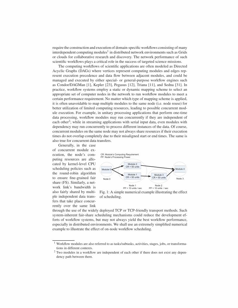
Fig. 1: A simple numerical example illustrating the effect
of scheduling.
Generally, in the case
of concurrent module ex-
ecution, the node’s com-
puting resources are allo-
cated by kernel-level CPU
scheduling policies such as
the round-robin algorithm
to ensure fine-grained fair
share (FS). Similarly, a net-
work link’s bandwidth is
also fairly shared by multi-
ple independent data trans-
fers that take place concur-
rently over the same link
through the use of the widely deployed TCP or TCP-friendly transport methods. Such
system-inherent fair-share scheduling mechanisms could reduce the development ef-
forts of workflow systems, but may not always yield the best workflow performance,
especially in distributed environments. We shall use an extremely simplified numerical
example to illustrate the effect of on-node workflow scheduling.
1 Workflow modules are also referred to as tasks/subtasks, activities, stages, jobs, or transforma-
tions in different contexts.2 Two modules in a workflow are independent of each other if there does not exist any depen-
dency path between them.

As shown in Fig. 1, a workflow consisting of five modules is mapped to a network
consisting of four nodes. For simplicity, we only consider the execution time of Modules
1, 2, and 3. With a fair-share scheduler, the workflow takes 15 seconds to complete
along the critical path (i.e. the longest path of execution time) consisting of Modules 0,
1, 3, and 4. However, if we let Module 1 execute exclusively ahead of Module 2, the
completion time of the entire workflow is cut down to 10 seconds. This example reveals
that the workflow performance could be significantly improved if concurrent modules
on the same node are carefully scheduled.
The work in this paper is focused on task scheduling for Minimum End-to-end De-
lay (MED) in unitary processing applications under a given workflow mapping scheme.
We formulate this on-node workflow scheduling problem as an optimization problem
and prove it to be NP-complete. Based on the exact End-to-end Delay (ED) calcula-
tion algorithm, extED [17], we conduct a deep investigation into workflow execution
dynamics and propose a Critical Path-based Priority Scheduling (CPPS) algorithm that
allocates the node’s computing resources to multiple concurrent modules assigned by
the given mapping scheme to the same node to minimize the ED of a distributed work-
flow. We also provide an analytical upper bound of the ED performance improvement
when the critical path remains fixed during workflow scheduling. The proposed CPPS
algorithm is implemented and tested in both simulated and experimental network envi-
ronments. The performance superiority of CPPS is illustrated by extensive simulation
results in comparison with a traditional fair-share scheduling policy, and is further veri-
fied by proof-of-concept experiments based on a real-life scientific workflow for climate
modeling deployed and executed in a testbed network.
The rest of the paper is organized as follows. In Section 2, we conduct a survey
of related work on both workflow mapping and scheduling. In Section 3, we provide
a formal definition of the workflow scheduling problem under study. In Section 4, we
design the CPPS algorithm. In Section 5, we implement the proposed algorithm and
present both simulation and experimental results. We conclude our work in Section 6.
2 Related Work
In this section, we provide a brief survey of related work on workflow optimization.
There are two aspects of optimizing distributed tasks to improve the performance of
scientific workflows: i) assigning the component modules in a workflow to suitable
resources, referred to as workflow mapping3, and ii) deciding the execution order and
resource sharing policy among concurrent modules on computer nodes or processors,
referred to as workflow/task scheduling. Both problems have been extensively studied in
various contexts due to their theoretical significance and practical importance [7,28,30].
When network resources were still scarce in early years, workflow modules were
often mapped to homogeneous systems such as multiprocessors [6, 22]. As distributed
computing platforms such as Grids and clouds are rapidly developed and deployed,
research efforts have shifted to workflow mapping in heterogeneous environments to
3 The workflow mapping problem is occasionally referred to as a scheduling problem in the
literature. In this paper, we designate it specifically as a mapping problem to differentiate it
from the workflow/task scheduling problem under study.

utilize distributed resources at different geographical locations across wide-area net-
works [8, 9, 28]. However, several of these studies assume that computer networks are
fully connected [30] or only consider independent tasks in the workflow [10]. These as-
sumptions are reasonable under certain circumstances, but may not sufficiently model
the complexity of real-life applications in wide-area networks. In real workflow sys-
tems, a greedy or similar type of approach is often employed for workflow mapping.
For instance, Condor implements a matchmaking algorithm that utilizes classified ad-
vertisements (ClassAds) mechanism for mapping user’s applications to suitable server
machines [27]. Most existing mapping algorithms are centralized, but decentralized
methods are desired for higher scalability. More recently, Rahman et al. proposed an
approach to workflow mapping in a dynamic and distributed Grid environment using a
Distributed Hash Table (DHT) based d-dimensional logical index space [26].
Considering the limit in the scope and amount of networked resources, a reasonable
workflow mapping algorithm inevitably results in a mapping scheme where multiple
modules are mapped to the same node, which necessitates the scheduling of concur-
rent modules. On-node processor scheduling has been a traditional research subject for
several decades, and many algorithms have been proposed ranging from proportional,
priority-based, to fair share [18, 19], to solve scheduling problems under different con-
straints with different objectives. Most traditional processor scheduling algorithms con-
sider multiple independent processes running on a single CPU with a goal to optimize
the waiting time, response time, and turnaround time of individual processes, or the
throughput of the system. The multi-processor and multi-core scheduling on modern
machines has attracted an increasing amount of attention in recent years [21, 24].
Our work is focused on a particular scheduling problem to achieve MED of a DAG-
structured workflow in distributed environments under a given mapping scheme. A
similar DAG-structured project planning problem dated back to late 1950’s and was
tackled using Program/Project Evaluation Review Technique and Critical Path Method
(PERT/CPM) [14, 20]. PERM is a method to analyze the involved tasks in completing
a given project and identify the minimum time needed to complete the total project.
CPM calculates the longest path of planned activities to the end of the project, and
the earliest and latest that each activity can start and finish without making the project
longer. The workflow scheduling problem differs from the project planning problem in
that the computing resources are shared among concurrent modules and the execution
time of each individual module is unknown until a particular task scheduling scheme is
determined. This type of scheduling problems are generally NP-complete. Garey et al.
compiled a great collection of similar or related multi-processor scheduling problems
in [15], which were tackled by various heuristics such as list scheduling and simple
level algorithm [16].
In practical system implementations, concurrent tasks are always assigned the same
running priority since the fair share of CPU cycles is well supported by modern operat-
ing systems that employ a round-robin type of scheduling algorithms. However, in this
paper, we go beyond the system-inherent fair-share scheduling to further improve the
end-to-end performance of scientific workflows through the use of an on-node schedul-
ing strategy taking into account the global workflow structure and resource sharing
dynamics in distributed environments.

3 Workflow Scheduling Problem
In this section, we construct analytical cost models and formulate the workflow schedul-
ing problem, which is proved to be NP-complete.
3.1 Cost Models
We model a workflow as a Directed Acyclic Graph (DAG) Gw = (Vw,Ew), |Vw| = m,
where vertices represent computing modules starting from the start module w0 to the
end module wm−1. A directed edge ei, j ∈ Ew represents the dependency between a pair
of adjacent modules wi and w j. Module w receives a data input of size z from each of
its preceding modules and performs a predefined computing routine, whose computing
requirement (CR) or workload is modeled as a function of the aggregate input data sizes.
Module w sends a data output to each of its succeeding modules after it completes its
execution. In this workflow model, we consider a module as the minimal execution unit,
and ignore the inter-module communication cost on the same node. For a workflow with
multiple start/end modules, we can always convert it to this model by adding a virtual
start/end module with CR = 0 and connected to all the original start/end modules with
data transfer size z = 0.
We model an overlay computer network as an arbitrary weighted graph Gc =(Vc,Ec),consisting of |Vc|= n nodes interconnected by |Ec| overlay links. A normalized variable
PPi is used to represent the overall processing power of node vi without specifying its
detailed system resources. Link li, j from vi to v j is associated with a certain bandwidth
bi, j. It is assumed that the start module w0 serves as a data source on the source node vs
without any computation to supply all initial data needed by the application and the end
module wm−1 performs a terminal task on the destination node vd without any further
data transfer.
Based on the above models, we can use an existing mapping algorithm to compute
a mapping scheme under the following constraints on workflow mapping and execu-
tion/transfer precedence [17]:
– Each module/edge is required to be mapped to only one node/link.
– A computing module cannot start execution until all its required input data arrive.
– A dependency edge cannot start data transfer until its preceding module finished
execution.
A mapping scheme M : Gw → Gc is mathematically defined as follows:
M : Gw → Gc =
w → c,∀w ∈Vw,∃c ∈Vc;
l(ci′ ,c j′) ∈ Ec,
{
if wi → ci′ ,w j → c j′ ,e(wi,w j) ∈ Ew,0 ≤ i, j ≤ |Vw|− 1,0 ≤ i′, j′ ≤ |Vc|− 1.
(1)
Once a mapping scheme is obtained, we can further convert the above workflow and
network models to virtual graphs as follows: each dependency edge in the workflow is
replaced with a virtual module whose computational workload is equal to the corre-
sponding data size, and each mapped network link is replaced by a virtual node whose
processing power is equal to the corresponding bandwidth. This conversion facilitates
workflow scheduling as we only need to focus on the module execution time. We use tsw

Table 1: Parameters in the cost models and algorithm design.
Parameters Definitions
Gw = (Vw,Ew) a computing workflow
m the number of modules in the workflow
wi the i-th computing module
w0 the start computing module
wm−1 the end computing module
ei, j the dependency edge from module wi to w j
z the data size of dependency edge e
CRi the computing requirement of module wi
Gc = (Vc,Ec) a computer network
n the number of nodes in the network
vi the i-th network of computer node
vs the source node
vd the destination node
PPi the processing power of node vi
li, j the network link from node vi to v j
bi, j the bandwidth of link li, j
and tfw to denote the execution start and finish time of module w. For convenience, we
tabulate the notations used in the cost models in Table 1, some of which will be used in
the algorithm design.
3.2 Problem Definition
Since the start time of a module in the workflow depends on the end time of its preceding
module(s), even independent modules assigned to the same node may not always run
in parallel. Therefore, task scheduling is only applicable to concurrent modules that run
simultaneously at least for a certain period of time. We formally define the On-Node
Workflow Scheduling (ONWS) problem as follows:
Definition 1. (ONWS) Given a DAG-structured computing workflow Gw = (Vw,Ew),a heterogeneous overlay computer network Gc = (Vc,Ec) and a mapping scheme M :
Gw → Gc, we wish to find a job scheduling policy on every computer node with concur-
rent modules such that the mapped workflow achieves:
MED = minall possible job scheduling policies
(TED) . (2)
3.3 NP-Completeness Proof
We first transform the original ONWS problem to its decision version, referred to as
ONWS-Decision, with a set of notations commonly adopted in the definitions of tradi-
tional multi-processor scheduling problems in the literature.
Definition 2. (ONWS-Decision) Given a set T of tasks t, each having a length(t) and
executed by a specific processor p(t), a number m ∈ Z+ of processors, partial order ≺

on T, and an overall deadline D ∈ Z+, is there an m-processor preemptive schedule for
T that obeys the precedence constraints and meets the overall deadline?
Note that in Definition 2, the workflow in the original ONWS problem is expressed
as a set of tasks with a partial-order relation and the given mapping scheme is expressed
as a set of node assignments or requirements for all tasks. Also, we consider preemptive
scheduling in our problem. The difficulty of ONWS-Decision is given by Theorem 1,
which is proved by showing that the m-processor bound unit execution time (MBUET)
system scheduling problem in [16], an existing NP-complete problem as defined in
Definition 3, is a special case of ONWS-Decision.
Definition 3. (MBUET) Given a set T of tasks, each having length(t) = 1 (unit exe-
cution time) and executed by a specific processor p(t), an arbitrary number m ∈ Z+ of
processors, partial order ≺ of a forest on T, and an overall deadline D ∈ Z+, is there an
m-processor schedule for T that obeys the precedence constraints and meets the overall
deadline?
Theorem 1. The ONWS-Decision problem is NP-complete.
Proof. Obviously, the MBUET scheduling problem is a special type of ONWS-Decision
problem with length(t) restricted to be 1 for all tasks t ∈ T and partial order ≺ restricted
to be a forest. For preemptive scheduling as considered in ONWS-Decision, a task is
not required to finish completely without any interruption once it starts execution. How-
ever, if we restrict the length of all tasks to be 1 (the smallest unit of time) in the input
of ONWS-Decision, each task would finish in its entirety once it is assigned to the des-
ignated processor for execution. Moreover, the partial order ≺ of a forest is a special
DAG structure of workflow topology. Therefore, the MBUET problem polynomially
transforms to the preemptive ONWS-Decision scheduling problem. Since MBUET is
NP-complete [16], the general ONWS-Decision problem is also NP-complete. The va-
lidity of the NP-completeness proof by restriction is established in [15], where “restric-
tion” constrains the given, not the question of a problem.
4 Algorithm Design
4.1 Analysis of Resource Sharing Dynamics in Workflows
Since the end-to-end delay (ED) of a workflow is determined by its critical path, i.e.
the path of the longest execution time, a general strategy for workflow scheduling is
to reduce the execution time of critical modules (i.e. modules on the critical path) by
allocating to them more resources than those non-critical modules that are running con-
currently. Ideally, the MED would be achieved if all possible execution paths from the
start module to the end module have the same length of execution time.
We first present a theorem on the resource sharing dynamics among the concurrent
modules assigned to the same node, which will be used in the design of our scheduling
algorithm.
Theorem 2. The finish time of the last completed module among k concurrent modules
executed on the same node with a single fully-utilized processor of processing power
PP is a constant,∑k
i=1 CRi
PP.

Proof. Since the total workload of all k modules is fixed, i.e. ∑ki=1 CRi, and the processor
is fully operating, no matter how the modules are scheduled, the total execution time
remains unchanged and is bounded by the finish time of the last completed module.
To understand the significance of workflow scheduling, we investigate a particular
scheduling scenario shown in Fig. 2 where the best performance improvement could be
achieved over a fair-share scheduling policy with the following conditions:
– There are k modules running concurrently on the same node v1 during their entire
execution time period;
– Among k modules, one is a critical module and k−1 are non-critical modules, and
all of them are of the same computing requirement (CR);
– Each non-critical module is the only module on its execution path (except for the
start and end modules).
1mw
sv 2v dv1v
0w
1w
kw
2w
Critical Path
Fig. 2: A scheduling scenario that achieves the upper bound performance.
Based on the scheduling scenario depicted in Fig. 2, we have the following theorem:
Theorem 3. The workflow’s MED performance improvement of any on-node task schedul-
ing policy with a fixed critical path over fair share is upper bounded by 50%.
Proof. We first justify that the conditions in Fig. 2 are necessary for achieving the upper
bound of the workflow’s MED improvement.
Let x be the original execution time of the critical module on v1 using the fair-share
scheduling policy. If there were any non-critical modules on v1 that finished before x,
even if we let the critical module w1 run exclusively first, it would take longer than xk
to complete. Thus, we would not be able to reduce the execution time of the critical
module to the minimum time possible, i.e. xk. On the other hand, if there were any non-
critical modules on v1 that finished after x, from Theorem 2, we know that the total
execution time on this node would be greater than x, and hence we would not be able to
reduce the length of the critical path to x.
The above discussion concludes that all k modules on node v1 must share resources
during their entire execution time and finish at the same time x to achieve the maximum
possible reduction on the length of the critical path. Since we consider fair share as the
comparison base in Theorem 2, the CRs of all k modules must also be identical. In this
scheduling scenario, if we let the critical module w1 execute exclusively first, its finish

time tfw1
would be reduced from x to xk, which is the best improvement possible with k
concurrent modules on the same node.
We use y to denote the sum of the execution time for the rest of the modules on
the critical path (excluding w1). From Theorem 2, we have max(t fwi) = x, i = 2,3, . . . ,k,
which means that the latest finish time of the last completed non-critical module would
be still x. Since the new length of the critical path (i.e. MED) becomes xk+ y, the upper
bound MED improvement is achieved if this new length is equal to the latest finish time
of any non-critical module, i.e. xk+y = x. It follows that y = k−1
kx. Therefore, the MED
improvement over fair share is ∆ = (x+y)−x
x+y= k−1
2k−1, which is 1/2 or 50% as k → ∞.
4.2 Critical Path-based Priority Scheduling (CPPS) Algorithm
Algorithm 1 CPPS(Gw′, Gc
′, f )
Input: A converted workflow graph Gw′ =(Vw
′,Ew′), a converted network graph Gc
′ =(Vc′,Ec
′),a given mapping scheme f : Gw
′ → Gc′.
Output: the scheduling policies on all the mapping nodes.
1: Calculate the execution time TFS for all the modules in Gw′ using a fair-share scheme;
2: Calculate the critical path CPFS and its length T (CPFS) based on TFS;
3: Calculate the execution time TCPPS for all the modules in Gw′ using Alg. 2, which in turn
uses Alg. 3 to decide the priorities for all the modules;
4: Calculate the new CPCPPS and its length T (CPCPPS) based on TCPPS;
5: if T (CPCPPS)≥ T (CPFS) then
6: return the fair-share schedule and T (CPFS).7: else
8: return the new CPPS schedule and the ED T (CPCPPS) of the mapped workflow.
We propose a Critical Path-based Priority Scheduling (CPPS) algorithm to solve the
ONWS problem. The CPPS algorithm produces a set of processor scheduling schemes
for all mapping nodes that collectively cut down the execution length of the critical path
in the entire workflow to achieve MED.
The pseudocode of the proposed CPPS algorithm is provided in Alg. 1, which first
calculates the critical path based on the fair-share (FS) scheduling, and then uses Algs. 2
and 3 to compute the new task schedule of concurrent modules on each mapping node.
In most cases, the new schedule outperforms the FS schedule. However, if the new
schedule does not improve the MED performance, the CPPS algorithm simply rolls
back to the FS schedule.
In Alg. 2, we calculate the independent set of each module in line 8 and find the
set set0 of modules with the earliest start time in line 12. If there is only one module in
set0, this module is executed immediately; otherwise, a scheduling strategy needs to be
decided. In line 18, we recalculate the percent of processing power that is allocated to
those modules in set0. In lines 18-32, a new scheduling policy is generated and applied
to all concurrent modules.

Algorithm 2 extEDOnNode(Gw′, Gc
′, f , TFS, CPFS)
Input: A converted workflow graph Gw′ =(Vw
′,Ew′), a converted network graph Gc
′ =(Vc′,Ec
′),a mapping scheme f : Gw
′ → Gc′, the execution time TFS of each module under the fair-share
scheme, and the critical path CPFS based on TFS.
Output: the new execution time TCPPS of all modules and the ED T (CPCPPS) of the mapped
workflow.
1: ts(set): the set of start times of all the modules in a set;
2: t f (set): the set of finish times of all the modules in a set;
3: ids(w): the independent set of module w on the same node (excluding w);
4: est(set) = {w| w ∈ set and tsw = min(ts(set))}, i.e. the set of modules with the earliest start
time in a set;
5: ready(set) = {w| w ∈ set and w is “ready” to execute};
6: T BF(w): the partial workload of module w to be finished;
7: for all module wi ∈Vw′ do
8: Find ids(wi);9: Set wi as “un f inished”;
10: Set w0 as “ready”;
11: while exist “un f inished” modules ∈Vw′ do
12: Find set0 = est(ready(Vw′));
13: for all module wi ∈ set0 do
14: if |ids(wi)|== 0 then
15: Execute wi, calculate TCPPS(wi) and set wi as “ f inished”;
16: else
17: Find set1 = {w|w is “ready” and w ∈ est(ids(wi)∪wi)};
18: OnNodeSchedule(Gw′, Gc
′, f , TFS, TCPPS, wi ∪ ids(wi), CPFS);
19: Estimate t f (set1);20: Find set2 = {w | w ∈ ids(wi) & w /∈ set1, ts(w) < min(t f (set1)), and w is “ready”
and “un f inished”};
21: if |set2|> 0 then
22: for all module w j ∈ set1 do
23: From ts(w|w ∈ set1) to min(ts(set2)): 1) finish part of T BF(w j) with the new
scheduling policy determined in line 18; 2) calculate the partial amount of
TCPPS;
24: Update the new tsw j
= min(ts(set2));25: else
26: for all module w j ∈ set1 do
27: if tfw j
== min(t f (set1)) then
28: Execute w j , calculate TCPPS(w j), and set w j as “ f inished”;
29: else
30: From ts(w|w ∈ set1) to min(t f (set1)): 1) finish part of T BF(w j) with the
new scheduling policy determined in line 18; 2) calculate the partial amount
of TCPPS;
31: Update the new tsw j
= min(t f (set1));32: Mark all ready modules as “ready”;
33: Compute the CP based on the time components TCPPS(wi) for all wi ∈Vw′;
34: return the ED T (CPCPPS) of the mapped workflow.

Algorithm 3 OnNodeSchedule(Gw′, Gc
′, f , TFS, wi ∪ ids(wi), CPFS)
Input: A converted workflow graph Gw′ =(Vw
′,Ew′), a converted network graph Gc
′ =(Vc′,Ec
′),a given mapping scheme f : Gw
′ → Gc′, and a module set wi ∪ ids(wi) that combines wi and its
independent set ids(wi).Output: the percentage per(w) of resource allocation for all modules in wi ∪ ids(wi).
1: wcp: module of the critical path cp (i.e. critical module);
2: wnon cp: module that is not on the critical path (i.e. non-critical module);
3: per(w): percentage of processing power allocated to module w;
4: tOnNode: the estimated execution time of a module under the new scheduling strategy;
5: CP(w): the critical path (CP) consisting of module w;
6: CPL(w): the left CP segment from the start module to module w (i.e. the CP of the left-side
partial workflow ending at w);
7: CPR(w): the right CP segement from module w to the end module (i.e. the CP of the right-side
partial workflow starting at w);
8: LFT (ni): the latest possible finish time of concurrent modules assigned to node ni;
9: Texclusive(wi): execution time of wi when running exclusively on its mapping node map(wi);10: T BF(w): the partial workload of module w to be finished;
11: map(w): the node to which module w is mapped;
12: for all modules wi in wi ∪ ids(wi) do
13: Calculate CP(wi) = CPL(wi)+CPR(wi) based on TFS and TCPPS;
14: Find wcp = {w|CP(w) = max{CP(w)|w ∈ ids(wi)∪wi}};
15: Estimate execution time Texclusive(wcp);16: Calculate the latest possible finish time LFT (map(wi)) of modules mapped to map(wi);17: bool flag = false;
18: for all modules wi ∈ wi ∪ ids(wi) do
19: Estimate the amount of time Ttb f needed to finish T BF(wi);20: if wi is wnon cp then
21: ∆ t1 = min{LFT (map(wi))−Ttb f ,Texclusive(wcp)};
22: β = |{wk ∈CP(wi) and wk ∈ ∪{CP(w j)|w j ∈ ids(wi)}}|;23: if T (CP(wi))+β∆ t1 ≥ T (CPFS) then
24: f lag = true;
25: ∆ t2 = T (CPFS)−T (CP(wi));26: tOnNode = Ttb f +∆ t2;
27: Calculate per(wi) according to tOnNode;
28: mark wi;
29: if flag == true then
30: for all modules wi ∈ wi ∪ ids(wi) do
31: if wi is not marked in line 28 then
32: per(wi) =(
1−∑wi marked
wi∈wi∪ids(wi)per(wi)
)/(
∣
∣{wi ∪ ids(wi)}∣
∣−∣
∣{wi|wi marked}∣
∣
)
;
33: else
34: for all modules wi ∈ wi ∪ ids(wi) do
35: if wi is wcp then
36: per(wi) = 1.0;
37: else
38: per(wi) = 0.0;
39: return the ID of wi.
40: return per(wi) for all modules wi ∈ wi ∪ ids(wi).

Alg. 3 performs the actual on-node scheduling, where only two cases need to be con-
sidered: 1) when per(wcp) is 100% and other per(wnon cp) is 0%, 2) when all per(w)are between 0 and 100%. Whenever possible, we wish to run the critical module exclu-
sively first to cut down the length of the globe CP as much as possible. Accordingly,
Alg. 2 considers the following two possible scenarios for all modules wi ∈ wi ∪ ids(wi)depending on the output of Alg. 3:
1) When per(wcp) = 100% and per(wnon cp) = 0: since Alg. 3 returns the ID of
wcp, we execute the critical module wcp from the time point ts(w|w ∈ set1) to
min(ts(set2)) exclusively; while for other modules, we suspend them to wait for
wcp to finish. During this period of time, wcp may be entirely or partially com-
pleted. We then execute all unfinished modules (their unfinished part T BF(wi))that are mapped to node map(wcp) in a fair-share manner until the number of con-
current modules assigned to this node changes again.
2) When all per(w) are between 0 and 100%: we execute each module with its own
percent per(wi) of resource allocation until the number of concurrent modules
changes.
CR=40
CR=60
CR=80CR=10
CR=40
CR=20
CR=10
1w
2w4w
5w
6w
svdv
1( 10)v PP =
7w8w
3( 10)v PP =
2 ( 10)v PP =
3w
CR=0
0w
CR=0
Fig. 3: A simple numerical example used for illustrating the scheduling algorithms.
We shall use a simple numerical example to illustrate the CPPS scheduling process.
As shown in Fig. 3, a computing workflow consisting of nine modules w0,w1, . . . , and
w8 is mapped to a computer network consisting of 5 nodes vs,v1,v2,v3 and vd . The mod-
ules’ computing requirements (CR) and the nodes’ processing powers (PP) are marked
accordingly except for the start/end modules mapped to the source/destination nodes,
whose execution time is not considered (i.e. CR = 0).
As shown in Fig. 4, we first compute the execution start and end time TFS : tsw|t
fw of
each module under the fair-share (FS) scheduling policy. In this scheduling scenario,
the workflow takes 20 seconds to complete along the critical path (CP) consisting of
modules w0,w2,w4,w5,w7, and w8.
Now we describe the CPPS scheduling process. Fig. 5 illustrates the scheduling
status when modules w3 and w4 are being scheduled in the CPPS algorithm. At this
point of time, the left shadowed part has been scheduled by CPPS while the right shad-
owed part is still estimated based on FS. Note that the module start time tsw is always
counted from the point when the module is ready to execute, not from the point when
it actually starts execution. Right after w1 finishes execution, both w3 and w4 are ready
to execute with possible resource sharing. To decide the scheduling between them, we

8 | 14
2 | 60 | 2
16 | 208 | 16
7 | 80 | 7
0w1w
2w 4w
5w
6w
svdv
1( 10)v PP =
7w
8w
3( 10)v PP =2 ( 10)v PP =
3w
( ) : |s f
FS w wT w t t
CR=0CR=0
16 | 208 | 16
0 |
Fig. 4: The execution start time tsw and finish time t
fw of each module calculated under
the FS scheduling policy, listed in the form of TFS(w) : tsw|t
fw.
CR=0
0w
sv5 | 6
5 | 8
0 | 4
0 | 5
6|14
5w
8 | 14
16|20
6w
7wCR=0
8w
dv
1w3w
2w 4w
1( 10)v PP 2( 10)v PP
3( 10)v PP
( ) : |s f
CPPS w wT w t t ( ) : |s f
FS w wT w t t
4( )LCPw
4( )R
CP w
3( )R
CP w3( )
LCPw
Fig. 5: The scheduling status when modules w3 and w4 are being scheduled in the CPPS
algorithm. The left shadowed part has been scheduled by CPPS while the right shad-
owed part is estimated based on FS.
need to compute the longest (critical) path that traverses each of them by concatenating
the left and right segments of its critical path. For w3, the length of its left CP segment
(w0, w1, and w3), denoted as CPL(w3), is 5 under CPPS, while the length of its right
CP segment (w3, w7, and w8), denoted as CPR(w3), is 8 (including its own execution
time), which is estimated using the FS-based measurements in Fig. 4. Similarly, for w4,
the lengths of its left and right CP segments are 5 under CPPS and 13 based on FS
as shown in Fig. 4, respectively. Since CP(w4) = CPL(w4) +CPR(w4) = 18 is longer
than CP(w3) = CPL(w3)+CPR(w3) = 13, w4 is to be executed exclusively first. It is
estimated that the length of CP(w3) would not exceed the length of the original global
CPFS based on FS, which is 20, even if we let w4 run to its completion with exclusive
CPU utilization, so in this case, we assign the entire CPU to w4 until it finishes; oth-
erwise, w4 would execute exclusively until a certain point and then share with w3 in a
fair manner such that the length of CP(w3) does not exceed the length of the original
global CPFS based on FS. The new execution time of w3 and w4 is updated in Fig. 5.
This scheduling process is repeated on every mapping node until all the modules are
properly scheduled.
5 Performance Evaluation
We evaluate the performance of the proposed CPPS algorithm in both simulated and ex-
perimental network environments in comparison with the fair-share scheduling policy,
which is commonly adopted in real systems.

5.1 Simulation-based Performance Comparison
Simulation Settings In the simulation, we implement the CPPS algorithm in C++ and
run it on a Windows 7 desktop PC equipped with Intel(R) Core(TM)2 Duo CPU E7500
of 2.93GHz and 4.00GB memory.
We develop a separate program to generate test cases by randomly varying the prob-
lem size denoted as a three-tuple (m, |Ew|,n), i.e. m modules and |Ew| edges in the work-
flow, and n mapping nodes in the network. For a given problem size, we randomly vary
the module complexity and data size within a suitably selected range of values, and cre-
ate the DAG topology of a workflow as follows: 1) Lay out all the modules sequentially;
2) For each module, create an input edge from a randomly chosen preceding module
and create an output edge to a randomly chosen succeeding module (note that the start
module has no input and the end module has no output); 3) Repeatedly pick up a pair
of modules on a random basis and add a directed edge from left to right between them
until we reach the given number of edges.
Given the workflow structure and the number of mapping nodes with randomly
generated processing power, we randomly generate the mapping scheme but with some
specific topological constraints. In observation of the topological structures of real net-
works such as ESnet [2] and Internet2 [3], we first topologically sort all modules and
then map the modules from each layer of the workflow to the nodes that are within the
proximity of the corresponding layer in the network. In the same layer with multiple
modules/nodes, a greedy approach is adopted for node assignment.
Note that in the network, we do not need to specify the number of links as a param-
eter because there must exist a link between two mapping nodes where two adjacent
modules are mapped to ensure the feasibility of the given mapping scheme. A random
bandwidth is then selected from a suitable range of values and assigned to each link.
Since other links without any dependency edges mapped to will not affect the simula-
tion results, they are simply ignored.
Simulation Results To evaluate the performance of the proposed CPPS algorithm, we
randomly generate 4 groups of test cases with 4 different numbers of nodes, i.e. n =5,10,15, and 20. For each number of nodes (i.e. each group), we generate 20 problem
sizes, indexed from 1 to 20, by varying the number of modules from 5 to 100 at an
interval of 5 with a random number of edges.
For each problem size (m, |Ew|,n), we generate 10 random problem instances for
workflow scheduling with different module complexities, data sizes, node processing
powers, link bandwidths, and mapping schemes, and then calculate the average of the
performance measurements under both fair-share (FS) and CPPS scheduling. The MED
performance improvement or speedup of CPPS over FS, defined asTFS−TCPPS
TFS× 100%,
is tabulated in Table 2. Note that for the problem size indexed by 1 with m = 5, when
n > m (i.e. n = 10,15, and 20), the mapping scheme maps each module one-to-one to
a different node without any resource sharing, and hence the scheduling is not appli-
cable (marked by “–” in the table); so are the cases for the problem size indexed by
2 with m = 10 and n = 15 and 20, and the problem size indexed by 3 with m = 15
and n = 20. The average performance improvement measurements together with their
corresponding standard deviations are plotted in Fig. 6.

Table 2: MED improvement percentage of CPPS over FS.
Prb Num of Mods MED Improvement Percentage (%)
Idx m n=5 n=10 n=15 n=20
1 5 0.4023 – – –
2 10 9.3800 0.0834 – –
3 15 12.2844 4.1384 1.5431 –
4 20 12.3537 6.9193 9.2536 5.2417
5 25 12.8543 7.9172 11.3095 5.3134
6 30 13.6095 11.3572 11.7418 5.7544
7 35 14.0034 11.7431 13.4203 7.8624
8 40 15.4378 12.8595 13.5076 8.9894
9 45 15.3575 13.0498 13.8334 11.4692
10 50 18.8860 14.2790 11.1567 12.6608
11 55 17.8824 12.8271 13.1352 14.1371
12 60 14.6911 14.6843 14.1821 12.6241
13 65 17.3636 20.5909 16.7078 13.6390
14 70 17.1467 17.5231 17.9146 15.1107
15 75 15.9394 19.3904 16.6014 13.4181
16 80 21.3327 18.2815 18.5939 13.8302
17 85 17.8155 22.2571 18.8757 17.4691
18 90 19.0516 19.2820 17.6146 17.1279
19 95 18.7070 19.0163 17.6803 16.8793
20 100 20.2888 19.0798 18.4336 19.3523
1 3 5 7 9 11 13 15 17 19 0%
5%
10%
15%
20%
25%
30%
Problem Index (n=5)
Imp
rove
me
nt
Pe
rce
nta
ge
(FS
−C
PP
S)/
FS
× 1
00
%
1 3 5 7 9 11 13 15 17 19 0%
5%
10%
15%
20%
25%
30%
Problem Index (n=10)
Imp
rove
me
nt
Pe
rce
nta
ge
(FS
−C
PP
S)/
FS
× 1
00
%
1 3 5 7 9 11 13 15 17 19 0%
5%
10%
15%
20%
25%
30%
Problem Index (n=15)
Imp
rove
me
nt
Pe
rce
nta
ge
(FS
−C
PP
S)/
FS
× 1
00
%
1 3 5 7 9 11 13 15 17 19 0%
5%
10%
15%
20%
25%
30%
Problem Index (n=20)
Imp
rove
me
nt
Pe
rce
nta
ge
(FS
−C
PP
S)/
FS
× 1
00
%
Fig. 6: MED improvement of CPPS over FS.

The space for performance improvement largely depends on the given mapping
scheme. In small problem sizes, or when the number of modules is comparable to the
number of nodes, the modules are likely to be mapped to the nodes in a uniform manner,
resulting in a low level of resource sharing, unless there exist some nodes whose pro-
cessing power are significantly higher than the others in the network. Hence, in these
cases, the MED improvement of CPPS over FS is not very obvious. However, as the
problem size increases, more modules might be mapped to the same node with more re-
source sharing, hence leading to a higher performance improvement. This overall trend
of performance improvement is clearly reflected in Fig 6.
5.2 Proof-of-concept Experimental Results Using Climate Modeling Workflow
Weather Research and Forecasting (WRF) The Weather Research and Forecasting
(WRF) model [29] has been widely used for regional to continental scale weather fore-
cast. It is also one of the most widely used limited-area model for dynamical down-
scaling of climate projection by global climate models to provide regional details.
The workflow for typical applications of WRF model takes multiple steps, including
data preparation and preprocessing, actual model simulation, and postprocessing. Each
step could be computationally intensive and/or involve a large amount of data trans-
fer and processing. For a specific climate research project, such procedures have to be
performed repeatedly, in the context of either routine short-term weather forecast, or
periodic re-initialization of model in dynamical downscaling over the length of a cli-
mate projection. Moreover, because of the chaotic nature of the atmospheric system
and unavoidable errors in the input data and the imperfection of the model, ensemble
approaches have to be adopted with a sufficiently large number of simulations, with
slight perturbations to initial conditions or physical parameters, to enhance the robust-
ness of the prediction, or to provide probabilistic forecast for problems of interest. Each
single simulation may require a full or partial set of preprocessing and postprocessing,
in addition to the model simulation. Collectively, a project in this nature may involve
the execution of an overwhelmingly large number of individual programs. A workflow-
based management and execution is hence extremely useful to automate the procedure
and efficiently allocate the resources to carry out the required computational tasks.
Climate Modeling Workflow Structure The WRF model [4] is able to generate two
large classes of simulations either with an ideal initialization or utilizing real data. In
our workflow experiments, the simulations are generated from real data, which usually
require preprocessing from the WPS package [5] to provide each atmospheric and static
field with fidelity appropriate to the chosen grid resolution for the model.
As shown in Fig. 7, the WPS consists of three independent programs: geogrid.exe,
ungrib.exe, and metgrid.exe. The geogrid program defines the simulation domains and
interpolates various terrestrial datasets to the model grids. The user can specify infor-
mation in the namelist file of WPS to define simulation domains. The ungrib program
“degrib” the data and writes them in a simple intermediate format. The metgrid program
horizontally interpolates the intermediate-format meteorological data that are extracted
by the ungrib program onto the simulation domains defined by the geogrid program.

The interpolated metgrid output can then be ingested by the WRF package, which con-
tains an initialization program real.exe for real data and a numerical integration program
wrf.exe. The postprocessing model consists of ARWpost and GrADs. ARWpost reads-
in WRF-ARW model data and creates output files for display by GrADS.
WPS WRF
External Data
Post processing
Static
Geographic
Data
Gridded Data ungrib.exe
metgrid.exe real.exe wrf.exe
geogrid.exe
namelist.wps ARWpost.exe GrADs.exe
Fig. 7: The WPS-WRF workflow structure for climate modeling.
sv dv
Data Size 1
Data Size 2
Data Size 3
1w 2w
3w 4w
5w 6w
dragon.cs.memphis.edu mouse.cs.memphis.edu cow.cs.memphis.edu
geogrid
.exe
geogrid1
.exe
geogrid2
.exe
Virtual
Start
ungrib
.exe
ungrib1.
exe
ungrib2.
exe
metgrid2
.exe
metgrid1
.exe
metgrid
.exe
real
.exe
wrf
.exe
real1
.exe
wrf1
.exe
Virtual
End
real2
.exe
wrf2
.exe
ARWpost
.exe
ARWpost1
.exe
ARWpost2
.exe
Critical Path
Fig. 8: The workflow mapping scheme for job scheduling experiments.
Experimental Settings and Results As shown in Fig. 8, in our experiments, we du-
plicate the entire WPS-WRF workflow to generate three parallel pipelines processing
three different instances of input data of sizes 106.03 MBytes, 106.03 MBytes, and
740.89 MBytes, respectively. The testbed network consists of five Linux PC worksta-
tions equipped with multi-core processors of speed ranging from 1.0 GHz to 3.2 GHz.
The computing requirement (CR) of each module and the processing power (PP) of
each computer are measured or estimated using the methods proposed in [32]. In view
of the computational complexity of each program, the scheduling experiments consider
a subset of the programs in the original workflow, i.e. ungrib.exe, metgrid.exe, real.exe
and wrf.exe, which serve as the main data processing routines. In the WPS part of each
pipeline, we bundle ungrib.exe and metgrid.exe into one module denoted as w1, w3, and
w5, respectively; while in the WRF part of each pipeline, we bundle real.exe and wrf.exe
into one module denoted as w2, w4, and w6, respectively. We map modules w1, w3, and
w5 to dragon.cs.memphis.edu, modules w2 and w4 to mouse.cs.memphis.edu, and mod-
ules w6 to cow.cs.memphis.edu. The virtual start and end modules are mapped to the
other two machines. The preprocessing program geogrid and postprocessing program
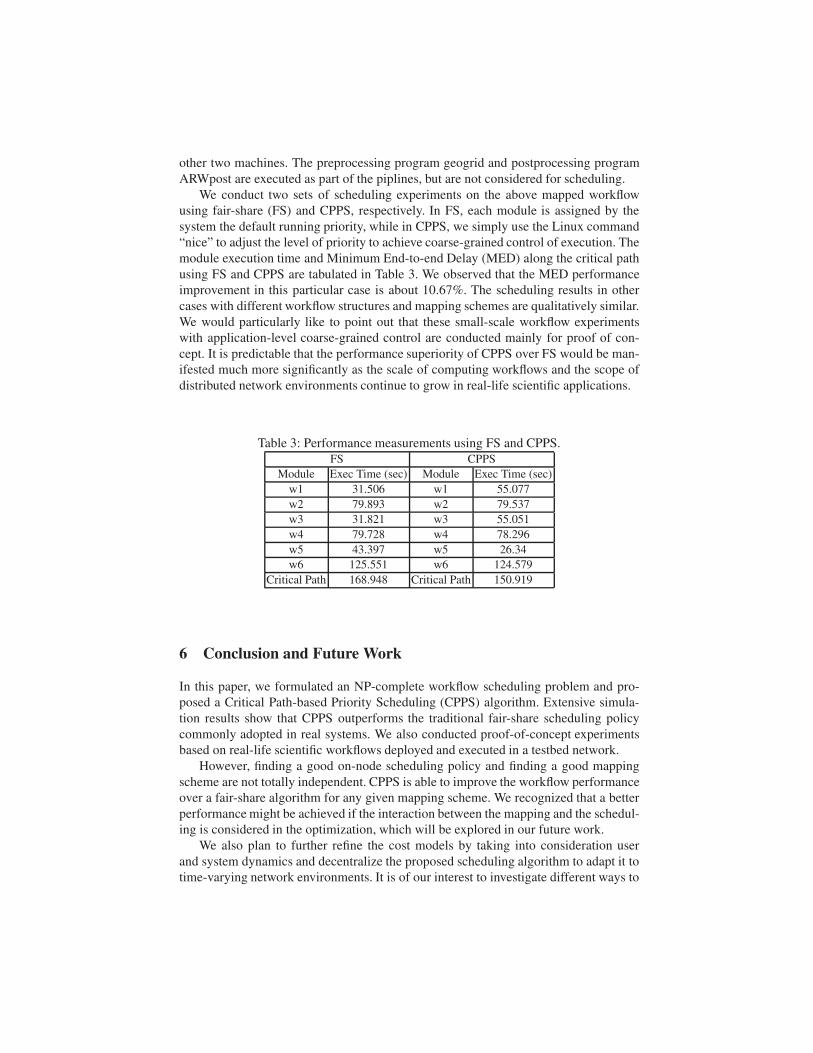
ARWpost are executed as part of the piplines, but are not considered for scheduling.
We conduct two sets of scheduling experiments on the above mapped workflow
using fair-share (FS) and CPPS, respectively. In FS, each module is assigned by the
system the default running priority, while in CPPS, we simply use the Linux command
“nice” to adjust the level of priority to achieve coarse-grained control of execution. The
module execution time and Minimum End-to-end Delay (MED) along the critical path
using FS and CPPS are tabulated in Table 3. We observed that the MED performance
improvement in this particular case is about 10.67%. The scheduling results in other
cases with different workflow structures and mapping schemes are qualitatively similar.
We would particularly like to point out that these small-scale workflow experiments
with application-level coarse-grained control are conducted mainly for proof of con-
cept. It is predictable that the performance superiority of CPPS over FS would be man-
ifested much more significantly as the scale of computing workflows and the scope of
distributed network environments continue to grow in real-life scientific applications.
Table 3: Performance measurements using FS and CPPS.
FS CPPS
Module Exec Time (sec) Module Exec Time (sec)
w1 31.506 w1 55.077
w2 79.893 w2 79.537
w3 31.821 w3 55.051
w4 79.728 w4 78.296
w5 43.397 w5 26.34
w6 125.551 w6 124.579
Critical Path 168.948 Critical Path 150.919
6 Conclusion and Future Work
In this paper, we formulated an NP-complete workflow scheduling problem and pro-
posed a Critical Path-based Priority Scheduling (CPPS) algorithm. Extensive simula-
tion results show that CPPS outperforms the traditional fair-share scheduling policy
commonly adopted in real systems. We also conducted proof-of-concept experiments
based on real-life scientific workflows deployed and executed in a testbed network.
However, finding a good on-node scheduling policy and finding a good mapping
scheme are not totally independent. CPPS is able to improve the workflow performance
over a fair-share algorithm for any given mapping scheme. We recognized that a better
performance might be achieved if the interaction between the mapping and the schedul-
ing is considered in the optimization, which will be explored in our future work.
We also plan to further refine the cost models by taking into consideration user
and system dynamics and decentralize the proposed scheduling algorithm to adapt it to
time-varying network environments. It is of our interest to investigate different ways to

implement the scheduling algorithm (at either the application or kernel level) and com-
pare their performances and overheads. We would also like to explore the possibilities
to integrate this scheduling algorithm into existing workflow management systems and
test it in wide-area networks with a high level of resource sharing dynamics.
Acknowledgments
This research is sponsored by U.S. Department of Energy’s Office of Science under Grant No. DE-
SC0002400 with University of Memphis.
References
1. DAGMan. http://www.cs.wisc.edu/condor/dagman
2. Energy Sciences Network. http://www.es.net
3. Internet2. http://www.internet2.edu
4. Http://www.wrf-model.org/index.php
5. WRF Preprocessing System (WPS). http://www.mmm.ucar.edu/wrf/users/wpsv2/wps.html
6. Annie, S., Yu, H., Jin, S., Lin, K.C.: An incremental genetic algorithm approach to multipro-
cessor scheduling. IEEE Trans. on Para. and Dist. Sys. 15, 824–834 (2004)
7. Bajaj, R., Agrawal, D.: Improving scheduling of tasks in a heterogeneous environment. IEEE
Trans. on Parallel and Distributed Systems 15, 107–118 (2004)
8. Benoit, A., Robert, Y.: Mapping pipeline skeletons onto heterogeneous platforms. In: Shi,
Y., van Albada, D., Dongarra, J., Sloot, P. (eds.) Int. Conf. on Computational Science, vol.
4487, pp. 591–598. Springer (2007)
9. Boeres, C., Filho, J., Rebello, V.: A cluster-based strategy for scheduling task on heteroge-
neous processors. In: Proc. of 16th Symp. on Comp. Arch. and HPC. pp. 214–221 (2004)
10. Braun, T., Siegel, H., Beck, N., Boloni, L., Maheswaran, M., Reuther, A., Robertson, J.,
Theys, M., Yao, B., Hensgen, D., Freund, R.: A comparison of eleven static heuristics for
mapping a class of independent tasks onto heterogeneous distributed computing systems.
JPDC 61(6), 810–837 (June 2001)
11. Churches, D., Gombas, G., Harrison, A., Maassen, J., Robinson, C., Shields, M., Taylor, I.,
Wang, I.: Programming scientific and distributed workflow with triana services. Concurrency
and Computation: Practice and Experience, Special Issue: Workflow in Grid Systems 18(10),
1021–1037 (2006), http://www.trianacode.org
12. Deelman, E., Blythe, J., Gil, Y., Kesselman, C., Mehta, G., Patil, S., Su, M., Vahi, K., Livny,
M.: Pegasus: mapping scientific workflows onto the grid. In: Proc. of the European Across
Grids Conference. pp. 11–20 (2004)
13. The office of science data-management challenge (Mar-May 2004), report of the DOE Office
of Science Data-Management Workshop. Technical Report SLAC-R-782, Stanford Linear
Accelerator Center
14. Fazar, W.: Program evaluation and review technique. The American Statistician 13(2), 10
(April 1959)
15. Garey, M., Johnson, D.: Computers and Intractability: A Guide to the Theory of NP-
completeness. W.H. Freeman and Company, San Francisco (1979)
16. Goyal, D.: Scheduling processor bound systems. Tech. rep., Computer Science Department,
Washington State University (1976)
17. Gu, Y., Wu, Q., Rao, N.: Analyzing execution dynamics of scientific workflows for latency
minimization in resource sharing environments. In: Proc. of the 7th IEEE World Congress
on Services. Washington DC (Jul 4-9 2011)

18. Henry, G.: The fair share scheduler. AT&T Bell Laboratories Technical Journal (1984)
19. Kay, J., Lauder, P.: A fair share scheduler. Communications of ACM 31(1), 44–55 (1988)
20. Kelley, J., Walker, M.: Critical-path planning and scheduling. In: Proc. of the Eastern Joint
Computer Conference (1959)
21. Kongetira, P., Aingaran, K., Olukotun, K.: Niagara: a 32-way multithreaded sparc processor.
IEEE Micro Magazine 25(2), 2129 (2005)
22. Kwok, Y., Ahmad, I.: Dynamic critical-path scheduling: An effective technique for allocating
task graph to multiprocessors. IEEE Trans. on Parallel and Distributed Systems 7(5), 506–
521 (May 1996)
23. Ludascher, B., Altintas, I., Berkley, C., Higgins, D., Jaeger-Frank, E., Jones, M., Lee, E.,
Tao, J., Zhao, Y.: Scientific workflow management and the Kepler system. Concurrency and
Computation: Practice and Experience 18(10), 1039–1605 (2006)
24. Mcnairy, C., Bhatia, R.: Montecito: A dual-core, dual-thread itanium processor. IEEE Micro
Magazine (2005)
25. Mezzacappa, A.: SciDAC 2005: scientific discovery through advanced computing. J. of
Physics: Conf. Series 16 (2005)
26. Rahman, M., Ranjan, R., Buyya, R.: Cooperative and decentralized workflow scheduling in
global grids. Future Generation Computer Systems 26, 753–768 (2010)
27. Raman, R., Livny, M., Solomon, M.: Resource management through multilateral matchmak-
ing. In: Proc. of the 9th IEEE Int. Symp. on High-Perf. Dist. Comp. (August 2000)
28. Ranaweera, A., Agrawal, D.: A task duplication based algorithm for heterogeneous systems.
In: Proc. of IPDPS. pp. 445–450 (2000)
29. Skamarock, W., Klemp, J., Dudhia, J., Gill, D., Barker, D., Duda, M., Huang, X.,
Wang, W., Powers, J.: A description of the advanced research wrf version 3. Tech. Rep.
NCAR/TN475+STR, National Center for Atmospheric Research, Boulder, Colorado, USA
(June 2008)
30. Topcuoglu, H., Hariri, S., Wu, M.: Performance effective and low-complexity task schedul-
ing for heterogeneous computing. IEEE TPDS 13(3) (2002)
31. Wassermann, B., Emmerich, W., Butchart, B., Cameron, N., Chen, L., Patel, J.: Workflows
for e-Science: Scientific Workflows for Grids, chap. Sedna: a BPEL-based environment for
visual scientific workflow modeling, pp. 427 – 448. Springer, London (2007)
32. Wu, Q., Datla, V.: On performance modeling and prediction in support of scientific workflow
optimization. In: Proc. of the 7th IEEE World Congress on Services. Washington DC (Jul 4-9
2011)